Article

An Off-Grid Compressive Sensing Algorithm Based on Sparse Bayesian Learning for RFPA Radar

School of Information and Electronics, Beijing Institute of Technology, Beijing 100081, China
*
Author to whom correspondence should be addressed.
Remote Sens. 2024, 16(2), 403; https://doi.org/10.3390/rs16020403
Submission received: 23 November 2023 / Revised: 13 January 2024 / Accepted: 18 January 2024 / Published: 20 January 2024
(This article belongs to the Special Issue Advanced Radar Signal Processing and Applications)

Abstract

:
In the application of Compressive Sensing (CS) theory for sidelobe suppression in Random Frequency and Pulse Repetition Interval Agile (RFPA) radar, the off−grid issues affect the performance of target parameter estimation in RFPA radar. Therefore, to address this issue, this paper presents an off−grid CS algorithm named Refinement and Generalized Double Pareto (GDP) distribution based on Sparse Bayesian Learning (RGDP−SBL) for RFPA radar that utilizes a coarse−to−fine grid refinement approach, allowing precise and cost−effective signal recovery while mitigating the impact of off−grid issues on target parameter estimation. To obtain a high-precision signal recovery, especially in scenarios involving closely spaced targets, the RGDP−SBL algorithm makes use of a three−level hierarchical prior model. Furthermore, the RGDP−SBL algorithm efficiently utilizes diagonal elements during the coarse search and exploits the convexity of the grid energy curve during the fine search, therefore significantly reducing computational complexity. Simulation results demonstrate that the RGDP−SBL algorithm significantly improves signal recovery performance while maintaining low computational complexity in multiple scenarios for RFPA radar.

1. Introduction

Random Frequency and Pulse Repetition Interval Agile (RFPA) radar effectively reduces the probability of interception by employing pseudo−random frequency and pulse repetition interval (PRI) [1]. By synthesizing a wideband spectrum, the anti−interference capabilities of the system are enhanced, and high resolution is achieved [2,3]. Furthermore, this radar avoids fixed ambiguous range and velocity measurements [4]. Consequently, in recent years, RFPA radar has emerged in the radar field as a prominent research topic [5].
However, applying matched filter methods to process RFPA radar echoes can result in sidelobes with a noise−like appearance in the range−velocity plane [6,7], where high sidelobe issues would possibly trigger false alarms or obscure smaller targets. Although preemptively designing the carrier frequency sequence [8,9] may mitigate sidelobe effects, this method does not account for scenarios involving multiple targets. As a result, it fails to guarantee that the superimposed sidelobes from multiple targets maintain a low level, severely affecting the sidelobe suppression performance. Therefore, sparse recovery based on the Compressive Sensing (CS) theory [10] offers a fresh perspective for RFPA radar sidelobe suppression and target parameter estimation, primarily for two reasons: (1) from the perspective of radar information acquisition, high sidelobe levels can be attributed to the information loss in the radar echoes [11]; and (2) parameter estimation in RFPA radar requires grid point division based on range and velocity resolution, resulting in sparsity in the observation scene due to significantly fewer observed data points compared to the potential grid points [12]. Therefore, many efforts have been made to employ CS−based sparse recovery algorithms for recovering RFPA radar signals [13], which achieves more effective sidelobe suppression compared to linear methods like matched filtering [14].
Currently, convex optimization algorithms and greedy algorithms are two primary CS−based sparse recovery algorithms for agile radar. Convex optimization algorithms, such as Basis Pursuit (BP) and Alternating Direction Method of Multipliers (ADMM), aim to transform the norm Nondeterministic Polynomial (NP) problem into a norm optimization problem to obtain a solution [15,16,17]. Greedy algorithms, including Orthogonal Matching Pursuit (OMP), continuously seek local optimal solutions to achieve a globally optimal solution [18,19]. However, when dealing with closely spaced targets in RFPA radar, the correlation between the columns of the observation matrix may be enhanced due to the overlapping echoes from nearby targets, affecting the reconstruction performance [20]. As a result, Sparse Bayesian Learning (SBL) algorithms have been proposed as a more robust alternative for sparse recovery in RFPA radar, utilizing Bayesian inference to model the sparsity and noise of signals as probability distributions [21,22]. The SBL algorithm was initially proposed in the field of machine learning [23]. In recent years, the SBL algorithm has been extensively applied in areas such as Direction of Arrival (DOA) estimation [24], radar imaging [25], and Multiple−Input Multiple−Output (MIMO) radar [26]. Since SBL considers the prior distribution of RFPA radar echoes and accounts for the correlation between columns of the observation matrix, it can enable robust reconstruction performance in scenarios with closely spaced targets [27]. However, SBL requires performing high−dimensional matrix inversions when computing the posterior covariance matrix in each iteration [22]. This increased computational requirement limits practical application when dealing with pulse−rich frequency−agile radar and large range−velocity observation data.
The CS algorithms mentioned above [15,16,17,18,19,21,22] are designed for on−grid scenarios in agile radar, assuming that targets are precisely located on predefined discrete grids. However, real targets may exist in a continuous domain between these grids, potentially leading to gridding errors in the estimation process. Consequently, when such off−grid issues arise, grid−based CS algorithms may distribute the energy of the RFPA signal across adjacent discrete grids, which may degrade reconstruction performance and, therefore, reduce the accuracy of target parameter estimation for RFPA radar [28,29]. Thus, researchers typically employ grid refinement, continuous−domain parameter estimation, or Bayesian learning−based methods to enhance reconstruction performance. These methods aim to make the conventional CS algorithms more robust in coping with mismatches between the actual signal parameters and the predefined discrete grids. For instance, Liu proposed the CS−Iterative Grid Optimization (CS−IGO) algorithm based on the norm [30]. Huang presented an Adaptive Matching Pursuit with Constrained Total Least Squares (AMP−CTLS) algorithm, which is based on the Matching Pursuit (MP) algorithm and can adaptively update grid points and observation matrix [31]. Additionally, Chen proposed a weighted Particle Swarm Optimization (PSO) algorithm based on the OMP algorithm [32]. Zhang utilized the atomic norm minimization algorithm to estimate parameters in a continuous domain, aiming to address the off−grid problem [33].
Nevertheless, current off−grid CS algorithms [30,31,32,33] in agile radar, primarily include greedy−based and convex optimization−based methods, exhibit relatively low reconstruction performance in scenarios involving closely spaced targets. Considering the superior signal recovery performance of the algorithms based on the SBL method under the on−grid assumption, especially in scenarios involving closely spaced targets, thus there is an emerging consideration to employ the SBL algorithm in off−grid situations. At present, in the field of radar, off−grid CS algorithms based on SBL are primarily applied in one−dimensional DOA estimation of array signals. Yang modeled the array manifold steering vector and proposed the Off−Grid Sparse Bayesian Inference (OGSBI) algorithm [34]. Dai introduced the Root-SBL algorithm, which utilizes roots of polynomials to eliminate the modeling error caused by off−grid issues, therefore enhancing computational efficiency [35]. Wang proposed the Grid Interpolation−Multiple snapshot SBL (GI−MSBL) algorithm, which employs grid interpolation to trisect between adjacent grid points, thus more accurately estimating the closely spaced off−grid DOA signals [36]. However, the above−mentioned off−grid algorithms based on SBL are applied in one−dimensional DOA estimation of array signals and are not directly applicable to the range−velocity estimation of RFPA radar targets. The primary reason for this limitation lies in the differences between their signal models. In DOA estimation, there is a uniformly arranged one−dimensional linear array, which simplifies the construction of the observation matrix. In contrast, in RFPA radar, the range and velocity parameters of targets are distributed on a two−dimensional range−velocity plane, and the signals also exhibit random carrier frequency and pulse repetition interval. These factors result in different methods for constructing observation matrices for each case, and directly applying the aforementioned algorithms for DOA estimation could adversely affect the effectiveness of sparse reconstruction. So, no off−grid SBL algorithm specifically tailored for range−velocity estimation of RFPA radar targets has been found in the literature. Moreover, the SBL algorithm facilitates the choice of diverse prior distributions for the original signal based on various observation scenarios [37], but the more complex the selected prior distribution is, the higher the computational complexity of subsequent processing will be. Therefore, it is crucial to explore innovative SBL−based off−grid CS methods that can maintain robust performance as well as computational feasibility in RFPA radar signal recovery, especially in scenarios involving closely spaced targets.
In this paper, we present an off−grid CS algorithm for RFPA radar named grid Refinement and Generalized Double Pareto (GDP) distribution based on SBL (RGDP−SBL) that combines SBL with grid refinement techniques, enabling accurate and robust signal recovery cost−effectively. As the SBL algorithm allows for the flexible selection of different prior distributions based on various observation scenarios to ensure accurate reconstruction performance, especially in scenarios involving closely spaced targets, a three−level hierarchical prior model is first employed to align the original signal of the RFPA radar with a GDP prior distribution. Then, the proposed RGDP−SBL algorithm utilizes a coarse−to−fine grid refinement approach for improved robustness, which can effectively alleviate the off−grid mismatch problem. Furthermore, the RGDP−SBL algorithm efficiently utilizes diagonal elements during the coarse search and takes advantage of the property that the grid energy curve approximates a convex function during the fine search, therefore reducing computational complexity. Simulation results show that this algorithm achieves more reliable recovery performance as well as computational feasibility, therefore enhancing the accuracy of target parameter estimation for RFPA radar, especially in scenarios involving closely spaced targets.

2. Materials and Methods

2.1. Signal Model

Given that an RFPA radar employs a rectangular pulse signal as the baseband signal, it encompasses N pulses within one Coherent Processing Interval (CPI). Furthermore, the RFPA radar scenario is stipulated to comprise noise and H moving point targets, each of which exhibits motion at a constant velocity along the radar line of sight. Consequently, the echo model for the n th pulse of the H targets can be described as follows [1]
S r ( n , t r ) = h = 1 H σ h r e c t ( t r , h 2 r h ( 0 ) c ( n + 1 U ( n ) ) T r ) × exp ( j 2 π f n ( t r , h 2 v h t r , h + 2 r h ( 0 ) c ( n + 1 U ( n ) ) T r ) + N t
For the h th target, the variable t r , h represents the time when the radar receives its echo. The parameters σ h and v h , respectively, denote the complex backward scattering coefficient and the radial velocity of the h th target, while r e c t represents the unit rectangle function. The initial distance between the h th target and the radar at time t = 0 is denoted by r h ( 0 ) , with c representing the speed of light. The average PRI is denoted by T r , where 1 / ( U ( n ) ) T r represents the PRI agility parameter of the n th pulse, following a uniform distribution 1 / U ( n ) 0 , 1 T w / T r , and T w is the pulse width. The frequency agility parameter of the n th pulse in RFPA radar is denoted by f n = f c + d n Δ f , where f c and Δ f are the central carrier frequency and the bandwidth of frequency−hopping step, respectively. The frequency−hopping code sequence d n { 0 , , M 1 } is a uniformly distributed code with M as frequency agility points [33,38]. N t represents the white Gaussian noise.
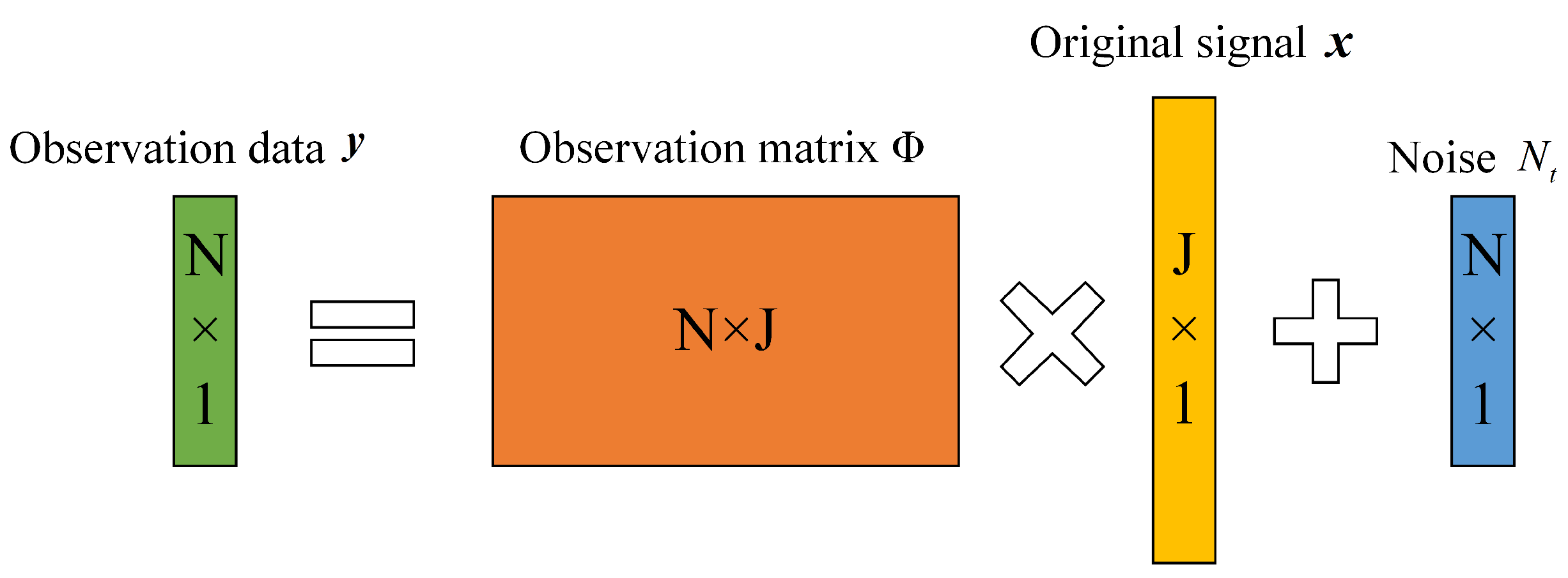
The RFPA radar achieves a larger synthetic bandwidth by changing the carrier frequency of each transmitted pulse. Specifically, the coarse−range cell is determined by the bandwidth of each transmitted pulse, while the fine−range cell is related to the final synthetic bandwidth. The sampled data of echoes is processed separately on different coarse−range cells [16]. As a result, the proposed algorithm in this paper focuses on only one coarse−range resolution cell. In the same coarse−range resolution cell, N pulse echoes are collected. The specific process of acquiring observation data is shown in Figure 1.
When only the coarse−resolution cell is considered, the target movement distance within the fast-time domain can be disregarded. Consequently, by isolating the phase term, adding the envelope σ h , and omitting the fast−time parameter, the n th sampled echo can be represented as
S r ( n ) = h = 1 H σ h exp ( j 4 π 1 c f c r h ( 0 ) ) exp ( j 4 π 1 c d n Δ f r h ( 0 ) ) × exp ( j 4 π 1 c f n v h ( n + 1 U ( n ) ) T r ) + N t
Then let
γ ˜ h = σ h exp ( j 4 π 1 c f c r h ( 0 ) ) p h = 4 π Δ f r h ( 0 ) d n / c q h = 4 π f c v h ( n + 1 U ( n ) ) T r ζ n / c ζ n = 1 + d n Δ f / f c
Here, the first term γ ˜ h can be considered to be a constant that is independent of pulse variations. The second term p h represents the range phase term and is related to d n in the pulse, which contains range information. The third term q h is the Doppler phase term, which varies with the pulse sequence n and contains velocity information. Therefore, Formula (2) can be rewritten as
S r ( n ) = h = 1 H γ ˜ h exp ( j p h ) exp ( j q h ) + N t
According to the derived signal model, the RFPA radar echoes exhibit sparsity characteristics in the range−velocity plane, as the number of targets within a coarse−resolution range cell is considerably fewer than the number of grid points. Hence, it is possible to utilize sparse recovery methods to discretize the range−velocity values into grid points, facilitating the design of the observation matrix and observation equation. Both the velocity and range values, initially continuous, are discretized into Q and P grid points, respectively. This process results in each range grid point being associated with Q velocity grid points, thus generating a total of P · Q = J grid points. As a result, the RFPA radar echo expression is divided into two parts, namely the range dimension R and the velocity dimension V, allowing us to construct the observation matrices for each dimension separately as follows:
Φ R C N × P = exp ( j 4 π 1 c f c R ) exp ( j 4 π 1 c d n Δ f R ) , R = R p 1 , , R p P Φ V C N × Q = exp ( j 4 π 1 c ( n + 1 U ( n ) ) T r ζ n f c V ) , V = V q 1 , , V q Q Φ C N × Q P = k r o n ( Φ R 1 , Φ V 1 ) k r o n ( Φ R N , Φ V N ) = Φ R p 1 1 · Φ V q 1 1 Φ R p P 1 · Φ V q Q 1 Φ R p 1 N · Φ V q 1 N Φ R p P N · Φ V q Q N , n = 1 , N
Here, Φ R and Φ V are the observation matrices for R and V, respectively. After performing the Kronecker operation on Φ R and Φ V , the final observation matrix, Φ can be obtained. According to the CS theory, the echo can be written as [10]
y = Φ x + N t
y = [ S r ( 1 ) , , S r ( N ) ] H C N × L is the known observation data composed of the received echoes with L snapshots, and x is the unknown original signal that contains both range and velocity information. The aforementioned process is illustrated in Figure 2.
In each pulse, the bandwidth of the frequency data in the received echoes is only 1 1 M M of the frequency agility range, thus leading to information loss. Therefore, Formula (6) represents an underdetermined equation, converting the range−velocity parameter estimation of the RFPA radar into a problem of solving an underdetermined equation in the CS framework. The objective of signal recovery is to reconstruct the signal x containing range and velocity information based on the known observation matrix Φ and the observed data composed of the received echoes y . Please note that the proposed algorithm takes y and Φ as inputs and then proceeds with the signal recovery [39].

2.2. Prior Distribution Assumption for Signals

The SBL algorithm assumes the original signal to be a random vector following a certain prior distribution, utilizing the Bayesian theorem to reconstruct the original signal [37,40]. Consequently, to enhance the recovery performance of the SBL algorithm, especially in scenarios involving closely spaced targets, it is essential to formulate a prior distribution assumption that exhibits superior sparsity. Currently, the prior distributions widely employed are complex Gaussian and Laplace distributions. The complex Gaussian distribution has fewer parameters and a simpler model but exhibits poorer sparsity. Utilizing the Laplace distribution increases the number of parameters but enhances the sparsity of the signal to a certain extent. Notably, the GDP distribution can be derived by adjusting the proportional mix of Laplace and complex Gaussian distributions. Moreover, the log-distribution function of the GDP prior forms a sharper concave peak compared to the aforementioned two prior distributions, therefore significantly enhancing sparsity [41]. Consequently, compared to complex Gaussian and Laplace distributions, the GDP distribution exhibits stronger sparsity and more flexible parametric forms, allowing for adjustments according to specific problems to achieve higher algorithmic performance. Therefore, the proposed algorithm in this paper assumes that the original signal follows the GDP distribution and its distribution function is of the form [41]
G D P ( x ; ρ , ε , μ ) = 1 2 ρ ( 1 + x μ ρ ε ) ( ε + 1 )
ρ is the scale parameter, ε is the shape parameter, and μ R is the location parameter. To ensure the GDP distribution serves as a convergent prior distribution, we set μ = 0 . Since the GDP distribution can only model real−valued signals, this paper adopts a three−level hierarchical prior model [42] to enable its application in the complex domain, thus facilitating the sparse recovery in RFPA radar. However, employing a more complex GDP distribution does introduce an increase in computational complexity. For this reason, the proposed algorithm utilizes methods that significantly mitigate computational complexity, with a comprehensive analysis of this process provided in Section 4.1.
In the first level of the prior distribution, it is assumed that elements in each column of the original signal x follow a zero-mean complex Gaussian distribution. Its Probability Density Function (PDF) can be written as
p ( x | γ ) = l = 1 L j = 1 J C N ( x j l | 0 , γ j ) = l = 1 L C N ( x l | 0 , Γ ) = π J L Γ L exp ( l = 1 L x l H Γ 1 x l )
γ = [ γ 1 , , γ J ] H is the hyperparameter of the original signal and γ j is the variance of the j th row. The covariance matrix of the original signal is expressed as Γ = d i a g ( γ j ) , and l 1 , . . . , L represents each snapshot in the RFPA radar echoes. In the second level of the prior distribution, to match the GDP distribution, it is assumed that each hyperparameter γ j in γ follows an independent Gamma distribution with a new hyperparameter ξ j . Thus, the PDF of hyperparameter γ can be obtained.
p ( γ | ξ ) = j = 1 J G a m m a ( γ j ; 3 2 , ξ j 2 4 )
G a m m a ( σ ; a , b ) = ( Γ ( a ) ) 1 b a σ a 1 exp ( b σ )
Γ ( a ) = 0 σ a 1 exp ( σ ) d σ
Here, ξ = [ ξ 1 , , ξ j ] H is the signal hyperparameter, and a and b are the parameters of the Gamma distribution. In the third level of the prior distribution, it is assumed that each hyperparameter ξ j in ξ follows an independent Gamma distribution. Hence, its PDF can be given as
p ( ξ ) = j = 1 J p ( ξ j ) = j = 1 J G a m m a ( δ , δ )
δ is a small positive constant tending to zero, and its value can be adjusted. As shown in [42], the probability distribution constituted by the three layers of hyperparameters follows a GDP distribution. Assuming that the noise in the RFPA radar echoes follows an independent complex Gaussian distribution, the RFPA radar echo y follows a complex Gaussian distribution, with its PDF given by
p ( y | x , β ) = l = 1 L C N ( y l | Φ x l , β 1 I )
β is the variance of the noise, and I is the identity matrix.

2.3. Coarse Search for RFPA Radar Targets

To perform a coarse search for RFPA radar targets based on the SBL framework, this section provides iterative formulas for the signal hyperparameters and noise variance, therefore laying a foundation for the subsequent fine search of the proposed algorithm. By integrating the likelihood with the prior based on the Bayesian theorem, the posterior PDF of the original signal x can be obtained.
p ( x | y ; Γ , β , ξ ) = p ( y | x , β ) p ( x | Γ ) p ( γ | ξ ) p ( ξ ) p ( y | x , β ) p ( x | Γ ) p ( γ | ξ ) p ( ξ ) d x
The posterior mean μ and variance Σ of x are given by [43] as follows:
μ = Γ Φ H Σ y 1 y Σ = Γ Γ Φ H Σ y 1 Φ Γ Σ y = β 1 I + Φ Γ Φ H
Σ y represents the covariance matrix of y . To determine the hyperparameters and noise variance, a Type II objective function is utilized for estimation [44]. The objective function following the GDP distribution can be written as
L II ( γ , ξ , β ) = p ( y | x , β ) p ( x | γ ) p ( γ | ξ ) p ( ξ ) d x
To derive the iterative formulas for the hyperparameters and noise variance, the Expectation−Maximization (EM) algorithm is employed to maximize Formula (16) [45,46]. The EM algorithm includes two steps: the Expectation step (E−step) and the Maximization step (M−step). In order to update the hyperparameters γ and ξ , the natural logarithm of the objective function is taken in the E−step, and the expectation is computed while neglecting the noise variance that is irrelevant to these two hyperparameters, which can be obtained as follows:
Q ( γ , ξ ) = Δ E p ( y | x ; γ , ξ , β ) { ln [ p ( y | x , β ) p ( x | γ ) p ( γ | ξ ) p ( ξ ) ] } = Δ E { ln [ p ( x | γ ) p ( γ | ξ ) p ( ξ ) ] } = E { ln [ π J L Γ L exp ( x H Γ 1 x ) j = 1 J G a m m a ( γ j ; 3 2 , ξ j 2 4 ) j = 1 J G a m m a ( ξ j ; δ , δ ) ] } j = 1 J { L ln γ j u j u j H + L Σ j j γ j ξ j 2 4 γ j + ln γ j + ln ξ j 3 δ ξ j + ( δ 1 ) ln ξ j }
Σ j j represents the element in the j th row and j th column of Σ , and u j is the vector of the j th row of the posterior mean u of the output signal for each iteration. In the M−step, the hyperparameters γ and ξ are updated separately to obtain the corresponding iterative formulas. First, let W j = 1 + Σ j j γ j ,thus the partial derivative of Formula (17) with respect to γ is calculated as
Q ( γ , ξ ) γ j = L W j γ j + u j u j H γ j 2 ξ j 2 4 + 1 2 γ j
Setting Formula (18) equal to zero yields the iterative formula for γ
γ j n e w = ( 2 L W j + 1 ) + 2 ( 1 / 2 + L W j ) 2 + u j u j H ξ j 2 ξ j 2
Σ j j = γ j ( γ j ) 2 ( Φ H Σ y 1 ) j Φ j
Similarly, the partial derivative of Formula (17) with respect to ξ can be written as
Q ( γ , ξ ) ξ j = ξ j 2 γ j δ + δ 1 ξ j + 3 ξ j
Setting Formula (21) equal to zero, we obtain the iterative formula for ξ
ξ j n e w = δ + δ 2 + 2 γ j ( δ + 2 ) γ j
The update process for the noise variance β follows the same steps as for the hyperparameters γ and ξ . In the E−step, the hyperparameters that are unrelated to the noise are ignored, resulting in the expectation form of the natural logarithm of the objective function as
Q ( β ) = Δ E p ( y | x ; γ , ξ , β ) { ln [ p ( y | x , β ) p ( x | γ ) p ( γ | ξ ) p ( ξ ) ] } = Δ E { ln [ p ( y | x , β ) ] } = N L ln ( π ) + N L ln ( β ) β ( y Φ μ F 2 + t r ( B B Σ y 1 B ) )
B = Φ Γ Φ H . In the M−step, the partial derivative of Formula (23) with respect to the parameter β is calculated as
Q ( β ) β = N L 1 β ( y Φ μ F 2 + t r ( B B Σ y 1 B ) )
Setting Formula (24) equal to zero yields the iterative formula for β
β n e w = N L ( y Φ μ F 2 + t r ( B B Σ y 1 B ) )
Thus, by using the aforementioned algorithm, the approximate location of the target in the range−velocity grid can be determined.

2.4. Fine Search for RFPA Radar Targets

Sparse recovery algorithms, by using non-linear methods that differ from matched filter algorithms, can relatively effectively enhance the resolution of RFPA radar and surpass the Rayleigh limit [11]. Thus, in this section, the algorithm searches between adjacent grid points on the grid obtained from coarse searching, updating their signal hyperparameters accordingly. According to Formula (16), considering only parameter γ , the cost function with respect to γ can be written as:
Θ ( γ ) = L ln Σ y l = 1 L ( y H Σ y 1 y ) + j = 1 J { ξ j 2 4 γ j + ln γ j }
Assuming the grid points obtained through coarse searching is ( R p , v q ) , the actual range−velocity of the target lies within the two−dimensional plane composed of ( R p 1 , v q 1 , R p + 1 , v q + 1 ) . To mitigate the impact of other targets, the fine search determines the refinement grid range for each target based on the results of the coarse search. In addition, the leakage of target energy into neighboring grid points can be eliminated by updating the signal hyperparameters. We define the number of grid points within the fine search range as k { 1 , , K } , and the corresponding observation matrix should be constructed as Φ ¯ ( k ) h . The signal covariance after leakage elimination is defined as Σ y h = Σ y Φ ˜ h γ h Φ ˜ h H , where Φ ˜ h and γ h are the observation matrix of the grid points around the h th target and the hyperparameters of the h th target, respectively. By updating Σ y h a second time, the signal covariance matrix after eliminating the influence of the new refined observation matrix is defined as Σ ¯ y = Σ y h + γ ¯ h Φ ¯ ( k ) h Φ ¯ ( k ) h H , where γ ¯ h is the hyperparameters associated with Φ ¯ ( k ) h . By replacing Σ y with Σ ¯ y , the following equation can be obtained.
Θ ( k , γ ¯ h ) = L ln Σ y h + γ ¯ h Φ ¯ ( k ) h Φ ¯ ( k ) h H l = 1 L y H ( Σ y h + γ ¯ h Φ ¯ ( k ) h Φ ¯ ( k ) h H ) 1 y ξ h 2 4 γ ¯ h + 1 2 ln γ ¯ h , k = 1 , , K
Let z h = Φ ¯ ( k ) h H Σ y h 1 Φ ¯ ( k ) h and q h = L Φ ¯ ( k ) h H Σ y h 1 R y   Σ y h 1 Φ ¯ ( k ) h . The updated equation for γ ¯ h can be obtained by setting the partial derivative of Θ ( k , γ ¯ h ) with respect to γ ¯ h to zero:
γ ¯ h = 2 ( ξ h 2 2 + L z h ) + 2 ( ξ h 2 2 + L z h ) 2 ξ h 2 ( L z h q h + ξ h 2 4 ) z h ξ h 2
Substituting γ ¯ h into Θ ( k , γ ¯ h ) , and choosing the point with the largest amplitude as the updated grid point, we have
k h n e w = arg max k h ( Θ ( k h ) )
( ) is the real part of Θ ( k h ) . By converting the obtained grid point into a range−velocity plane, the range and velocity parameters of the target can be determined. The process of the RGDP−SBL algorithm for RFPA radar is outlined in Algorithm 1.    
Algorithm 1: The Proposed RGDP−SBL Algorithm
1: Input: observed data composed of echoes y , error threshold ε , observation matrix Φ ,
    the number of snapshots L, the number of range−velocity grid points J, i t e r max ,
    pulse number N, parameter controlling the sparsity δ ,
2: Initialization: i t e r = 0 , γ 0 = 1 J L l = 1 L Φ H y , ξ 0 = 1 J × 1 , β 0 = N L 0.1 y 2 .
3: while i t e r i t e r max do
4:    i t e r = i t e r + 1 .
5:   Update μ i t e r and ( Σ j j ) i t e r by Formulas (15) and (20).
6:   Update γ i t e r and ξ i t e r by Formulas (19) and (22).
7:   Update β i t e r by Formula (25).
8:   if γ i t e r γ i t e r 1 2 γ i t e r 1 2 < ε
9:         break
10:        end
11: end while
12: Find H largest peak clusters in γ .
13: for h = 1 , , H do
14:        Update γ ¯ h by Formula (28).
15:        Update Θ ( k h , γ ¯ h ) by Formula (27).
16:        Update k h n e w by Formula (29).
17: end for
18: Output: μ , γ , k h n e w , converting the grid points k h n e w yields the range and velocity of the target.

3. Simulation Results

3.1. Simulation Setup

In this paper, simulations are conducted in two distinct cases: on−grid and off−grid. The on−grid simulations are utilized to analyze computational complexity and the performance of algorithms in scenarios involving closely spaced targets. Simultaneously, the off−grid simulations are conducted to compare the algorithms in terms of their ability to overcome off−grid issues. In the simulation setup shared across both on−grid and off−grid cases, the transmission signal is configured with a central carrier frequency of 10 GHz, an average PRI of 10 μ s, and 128 pulses in the same CPI. The bandwidth of the frequency−hopping step is set to 1 MHz, while the frequency agility range is configured at 128 MHz. The PRI agility range is configured at 5 μ s. The proposed algorithm is iterated up to 100 times during the simulation, with an error threshold ε set to 0.01. The value of the parameter controlling the sparsity δ will be examined in the subsequent section to determine the most suitable value. Additionally, in off−grid simulation, the search ranges for the coarse search are set at 2.5 m for range and 12.5 m/s for velocity, while the fine search employs search ranges of 0.1 m for range and 0.1 m/s for velocity. For clarity, the specific parameter settings of the RFPA radar are summarized in Table 1.
The Root Mean Square Error (RMSE) is employed to evaluate the performance of algorithms, and the range dimension R R M S E and the velocity dimension V R M S E are defined as
R R M S E = 1 M c H m c = 1 M c h = 1 H R ^ h m c R h m c 2 V R M S E = 1 M c H m c = 1 M c h = 1 H v ^ h m c v h m c 2
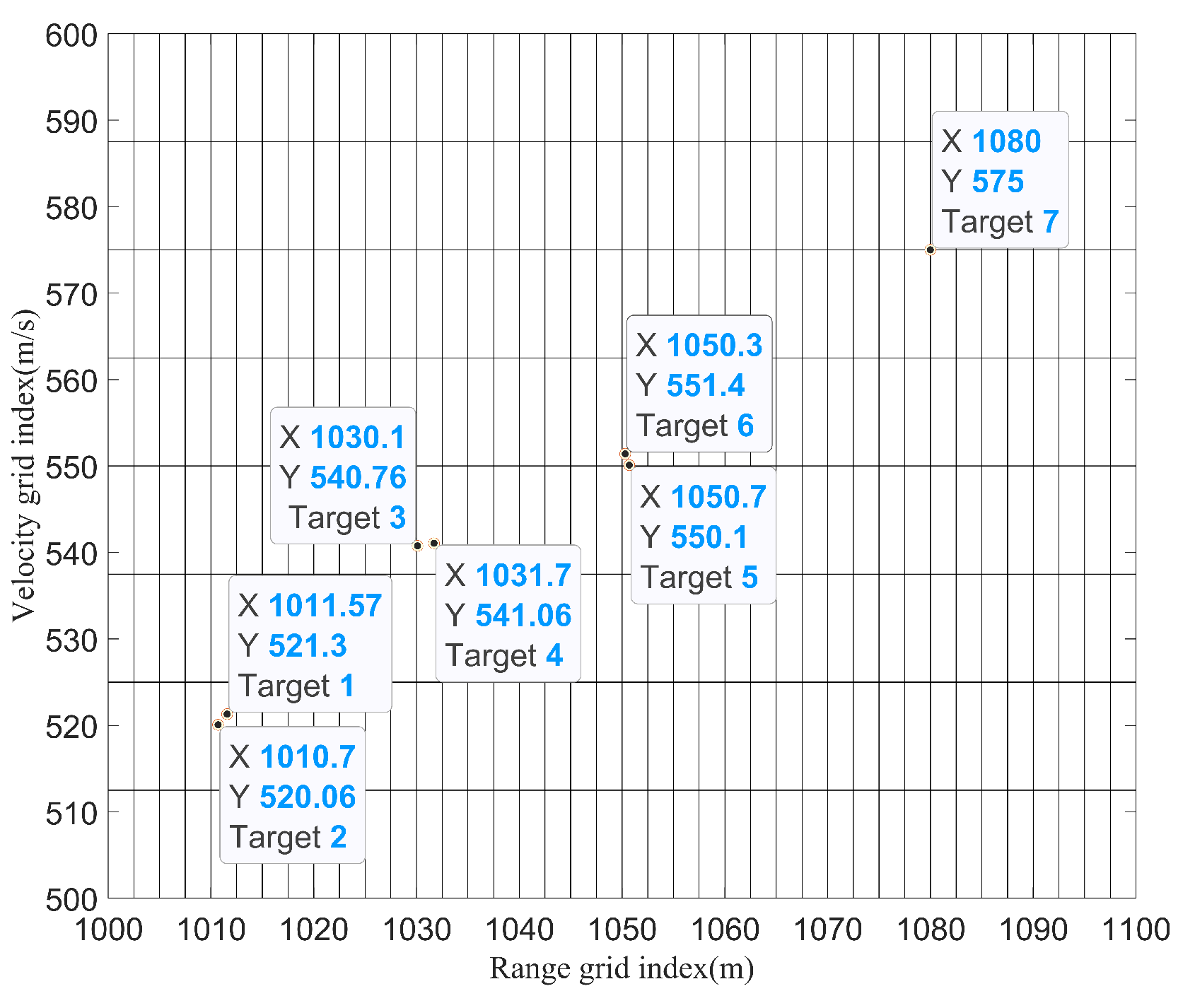
Here, M c is the number of Monte Carlo simulations, while H denotes the number of targets to be detected. v ^ and R ^ correspondingly represent the real velocity and range of the target, and v and R are the estimated velocity and range of the target, respectively. Please note that seven scenarios with different signal−to−noise ratio (SNR) are established in our simulation: (1) Scenario 1 is a single target scenario; (2) Scenario 2 consists of three targets within different range−velocity cells; (3) Scenario 3 involves three targets, with two in the same range−velocity cell, and is the main focus for further analysis; (4) Scenario 4 through Scenario 7 involve closely spaced targets with target numbers ranging from 4 to 7. Notably, to assess the performance of the proposed algorithm under on−grid and off−grid conditions, one target is set precisely on range−velocity grid points defined during the coarse search part in Scenario 2 to Scenario 7. The range and velocity of the target accurately located on grid points are 1080 m and 575 m/s. The parameters in each scenario are shown in Table 2.
As shown in Table 2, it is observed that some of the target parameters are shared from Scenario 3 to Scenario 7, and each target from Scenario 3 to Scenario 6 can be found in Scenario 7. Additionally, Scenario 2 includes three targets within different range−velocity cells. Therefore, for clarity, the positions of all targets in Scenario 2 and Scenario 7 with respect to the range−velocity grid defined during the coarse search part are illustrated in Figure 3 and Figure 4.
From Figure 3 and Figure 4, it can be observed that only Target 3 in Scenario 2 and Target 7 in Scenario 7 are precisely located on range−velocity grid points, while the other targets are not exactly positioned on range−velocity grid points. This arrangement facilitates the assessment of the performance of the proposed RGDP−SBL algorithm under on−grid and off−grid conditions in subsequent simulations.

3.2. GDP Parameters Analysis

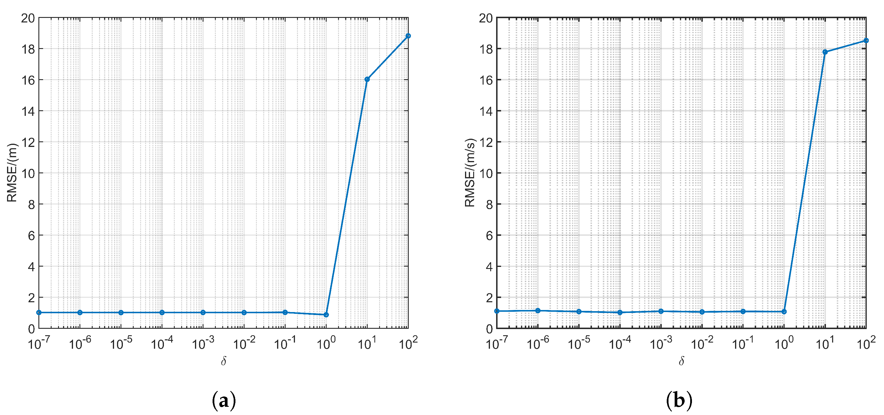
As the value of parameters δ controls sparsity [42], to enforce sparsity and improve signal reconstruction performance, we conducted a comprehensive analysis of the performance of the proposed algorithm under different values of δ in Formula (12). Simulations for the parameter δ , ranging from 10 7 to 100, are conducted under Scenario 3, with 200 independent Monte Carlo simulations performed for each value to calculate the results in terms of RMSE for range and velocity and the simulation results are presented in Figure 5.
As depicted in Figure 5, it is evident that when the value of δ is significantly large, the GDP distribution fails to effectively enhance sparsity, leading to a sharp increase in the RMSE for range and velocity. Conversely, when the value of δ falls within the range of 10 7 to 1, the proposed algorithm consistently exhibits superior performance with lower RMSE values for distance and velocity. Therefore, under the conditions of this simulation, any value of δ within the range of 10 7 to 1 can be selected. In the subsequent simulations in this paper, δ is set to 10 1 .

3.3. Performance Analysis under Off−Grid Conditions with On−Grid Assumption

In this section, to compare the performance of different algorithms in scenarios involving closely spaced targets under off−grid conditions, however, based on the on−grid assumption, two simulations are conducted under the on−grid assumption. In the simulation, first, the performance of SBL−based algorithms using different prior distributions is compared in various scenarios. A complex Gaussian distribution and a two-stage hierarchical form of Laplace distribution are employed to assess the performance of different prior distributions. Simultaneously, the coarse search parts of different algorithms are simulated in different scenarios. For comparison of different algorithms, four benchmark algorithms are employed: a greedy algorithm based on OMP, a convex optimization algorithm based on the ADMM algorithm, the SBL algorithm as described in [22], and the GI−MSBL algorithm in [36].

3.3.1. Impact of Performance Due to Different Prior Distributions

To validate the superiority of the proposed algorithm utilizing the GDP distribution in signal recovery in scenarios involving closely spaced targets, 200 Monte Carlo experiments are conducted using SBL−based algorithms with complex Gaussian distribution, Laplace distribution, and GDP distribution in Scenario 1, Scenario 2, and Scenario 3, respectively. The simulation results are shown in Table 3.
From Table 3, it can be observed that in Scenario 1, due to the simplicity of the observation scenario, the RMSE of each algorithm is at a relatively low level. However, as the observation scenarios become more complex and the targets become closer in range and velocity, the values of RMSE for algorithms using complex Gaussian and Laplace distributions sharply increase. In contrast, the values of RMSE for the algorithm using GDP distribution are less affected by changes in the observation scenario. This is attributed to the three−level hierarchical GDP distribution, which manifests higher sparsity in contrast to the other two distributions, therefore facilitating more accurate estimation of range and velocity parameters in scenarios involving closely spaced targets for RFPA radar.

3.3.2. Performance of Algorithms with the Coarse Search Parts

To compare the signal recovery performance of convex optimization algorithms, greedy algorithms, and SBL−based algorithms under the on−grid assumption in scenarios involving closely spaced targets, 200 Monte Carlo simulations are, respectively, conducted for the OMP algorithm, ADMM algorithm, SBL algorithm in [22], GI−MSBL algorithm, and the proposed algorithm in Scenario 1, Scenario 2, and Scenario 3. Please note that the simulations in this subsection are conducted under the on−grid assumption, and the OMP algorithm, GI−MSBL algorithm, and the proposed RGDP−SBL algorithm are integrated with grid refinement. Therefore, for a more objective comparison of the performance of each algorithm, it is sufficient to simulate only the coarse search part of the OMP algorithm, GI−MSBL algorithm, and the proposed RGDP−SBL algorithm. For clarity, OMP−C, GI−MSBL−C, and RGDP−SBL−C, respectively, denote the coarse search part of the corresponding algorithms. The simulation results are presented in Table 4.
It can be seen from Table 4 that under the on−grid assumption, the performance of the coarse search part of each algorithm is similar. It is worth noting that in Scenario 3, with closely spaced targets, the proposed RGDP−SBL algorithm has the best performance among all algorithms. Additionally, the RMSE of each algorithm is relatively large, indicating that under the on−grid assumption, the off−grid issues introduce significant errors, therefore affecting the performance of parameter estimation for RFPA radar. Therefore, it is essential to address the off−grid issue using grid mismatch techniques.

3.4. Performance Analysis under the Off−Grid Condition with Off−Grid Assumption

In this section, three simulations are conducted to assess the performance of various algorithms in overcoming the off−grid problem. For comparison, four benchmark algorithms in Section 3.3 are employed. Notably, the grid refinement approach for the OMP algorithm is based on the results of the coarse search part, with the refinement of the step in the range−velocity observation matrix to achieve grid refinement. However, in the existing literature, there are no specific ADMM or SBL algorithms incorporating grid refinement techniques for range−velocity estimation of RFPA radar in off−grid scenarios. Therefore, to ensure a more objective comparison, this study developed grid refinement algorithms for both the ADMM and SBL methods in [22] that are equivalent to the grid refinement approach used for the OMP algorithm. However, the OMP algorithm only restructures the observation matrix to achieve grid refinement. In contrast, the proposed RGDP−SBL algorithm conducts two rounds of hyperparameter updates during grid refinement, therefore eliminating the leakage of target energy into neighboring grid points and mitigating the influence of the newly refined observation matrix. For clarity, in subsequent simulations, OMP−G, ADMM−G, SBL−G, and GI−MSBL−G, respectively, denote the algorithms of each method utilizing grid refinement techniques.

3.4.1. Impact of Performance Due to Different Scenarios

Each algorithm is simulated in 200 Monte Carlo simulations in Scenario 1, Scenario 2, and Scenario 3, respectively, to assess the performance of each algorithm under different scenarios. The simulation results are presented in Table 5.
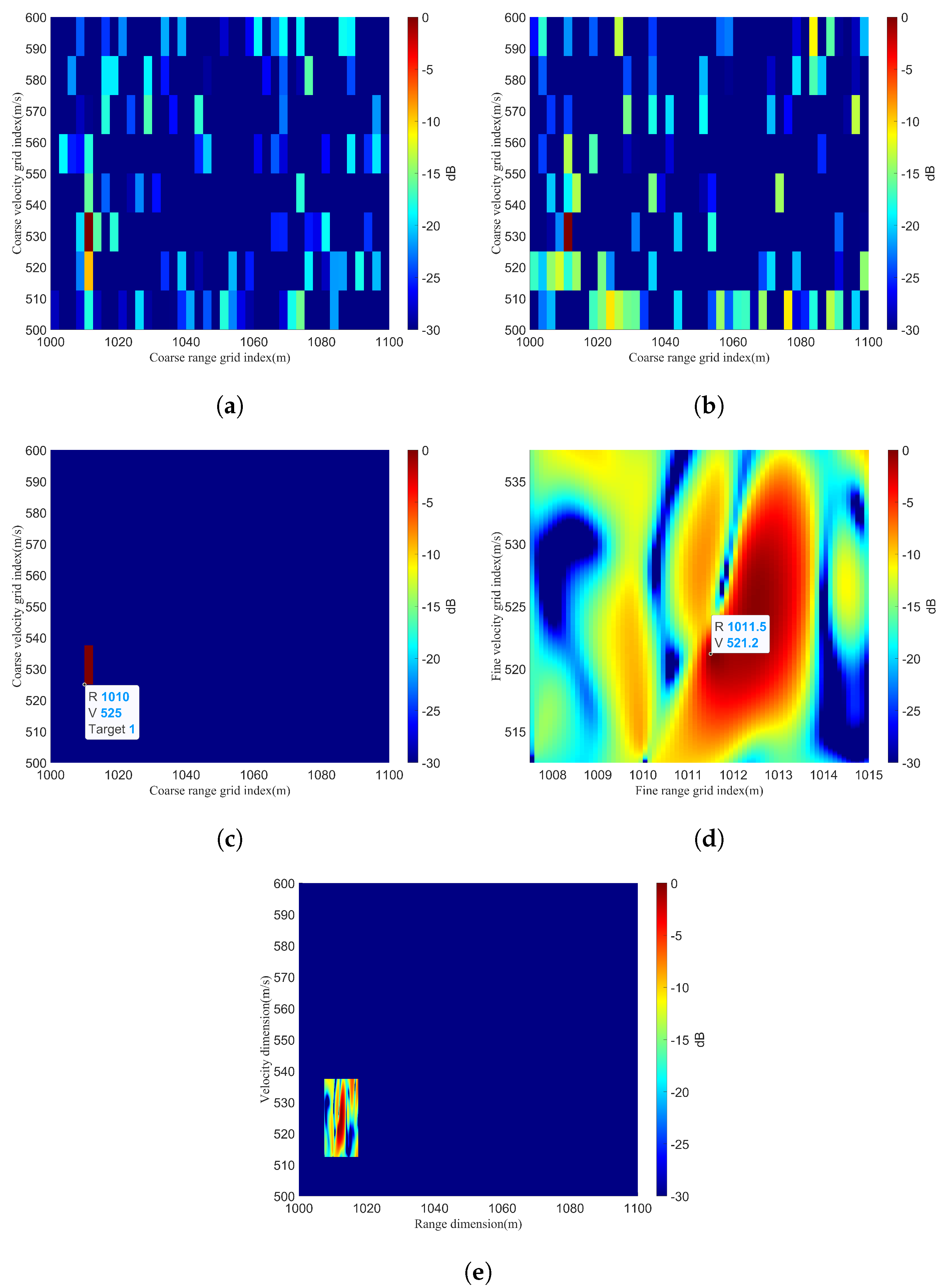
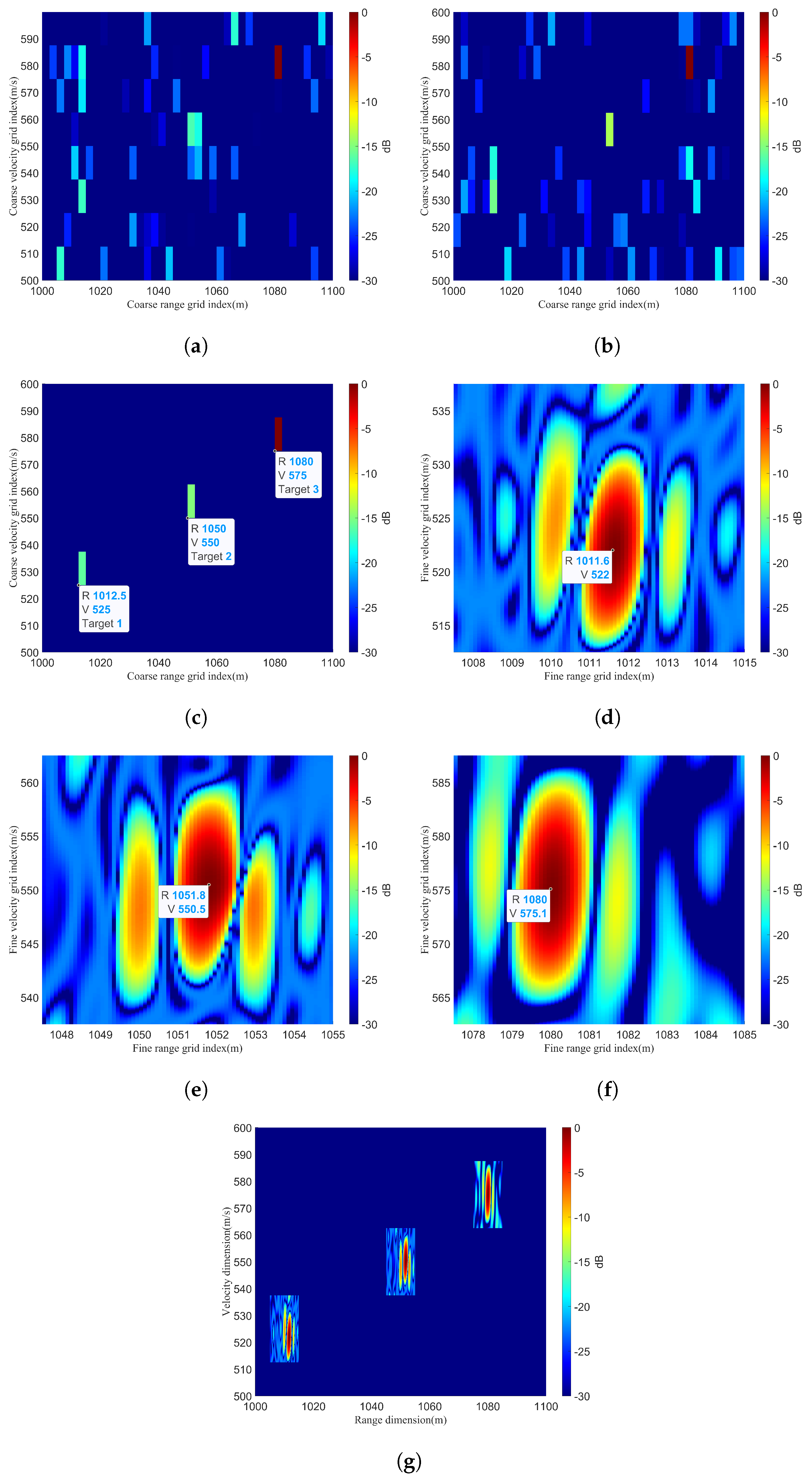
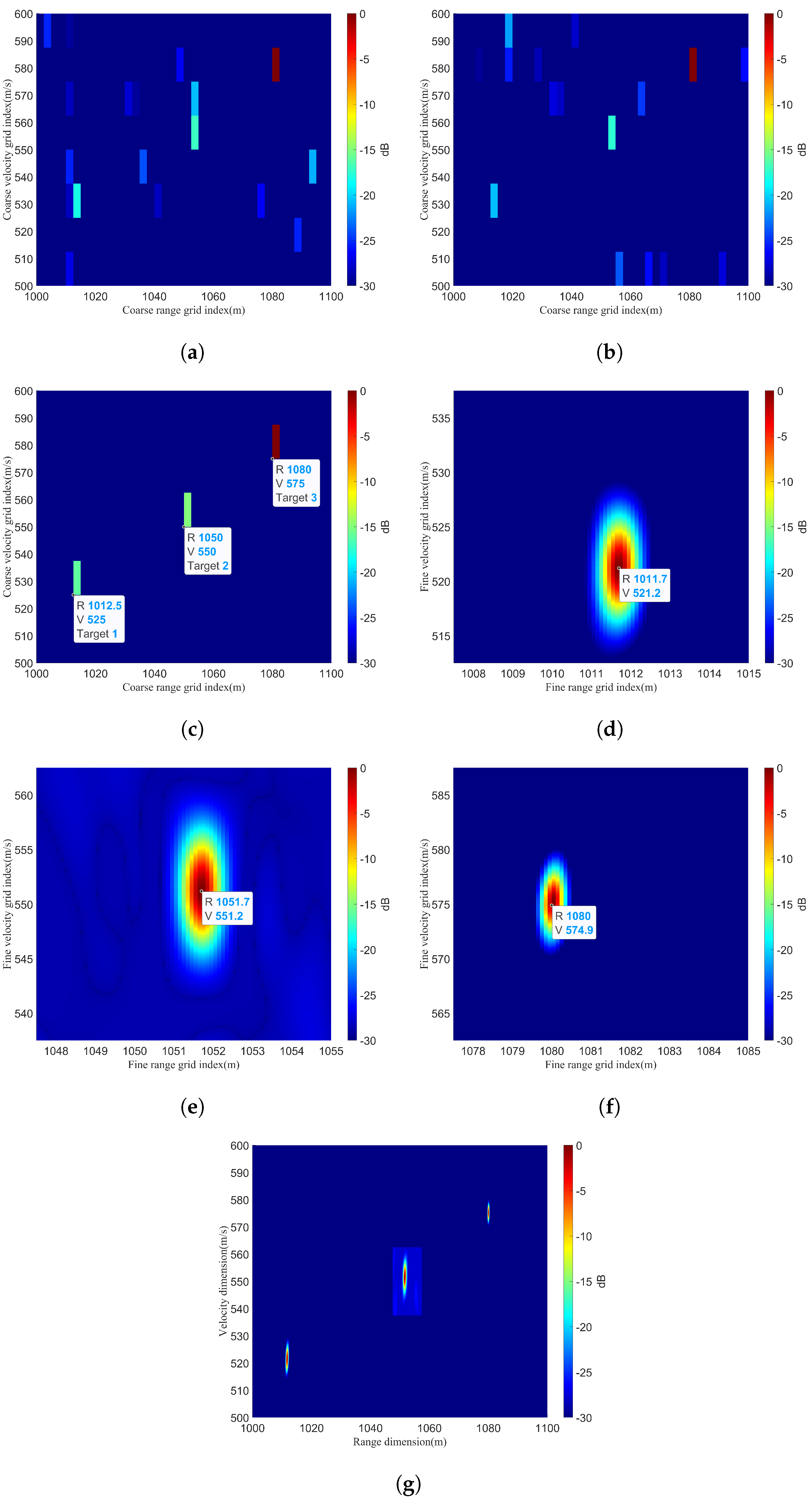
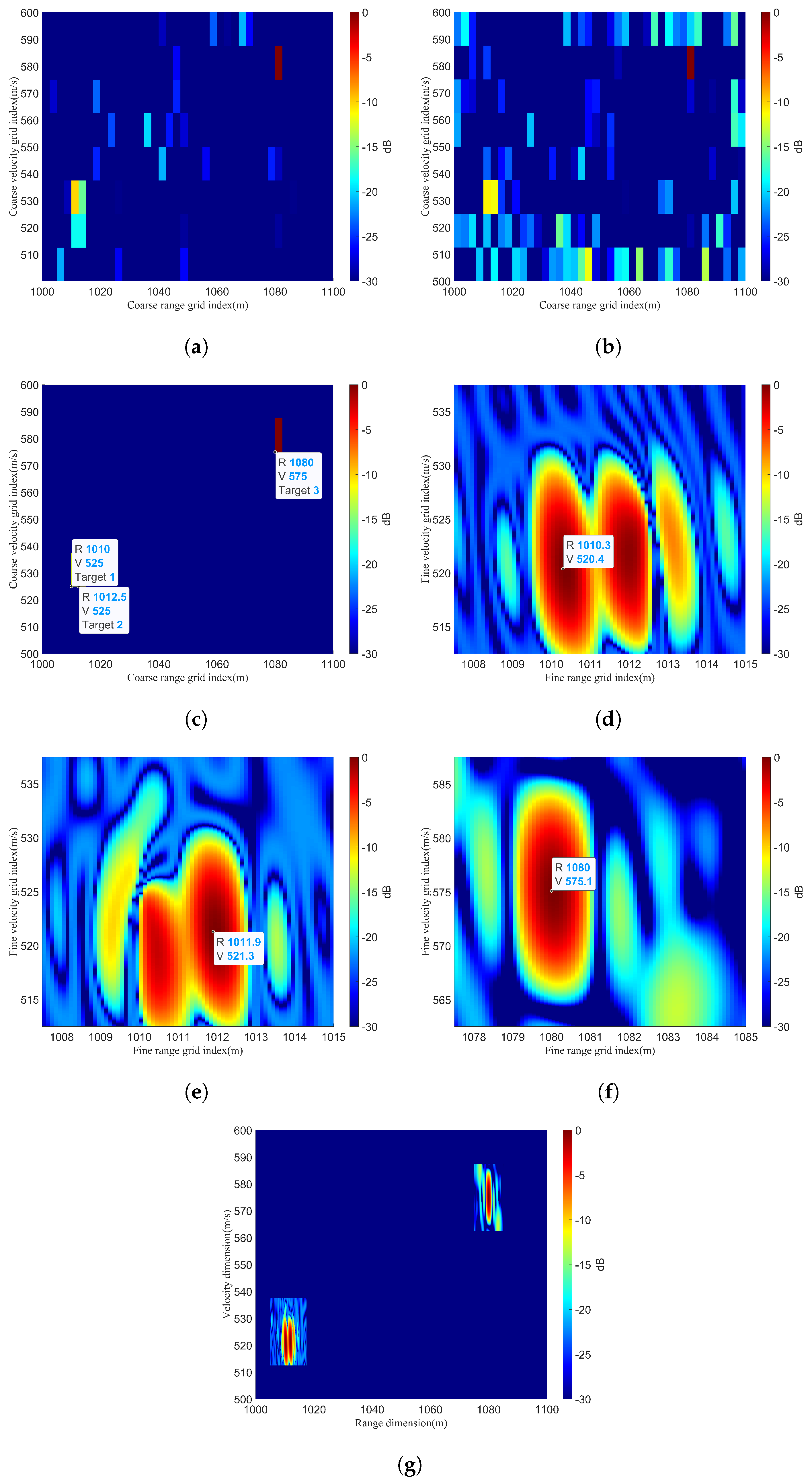
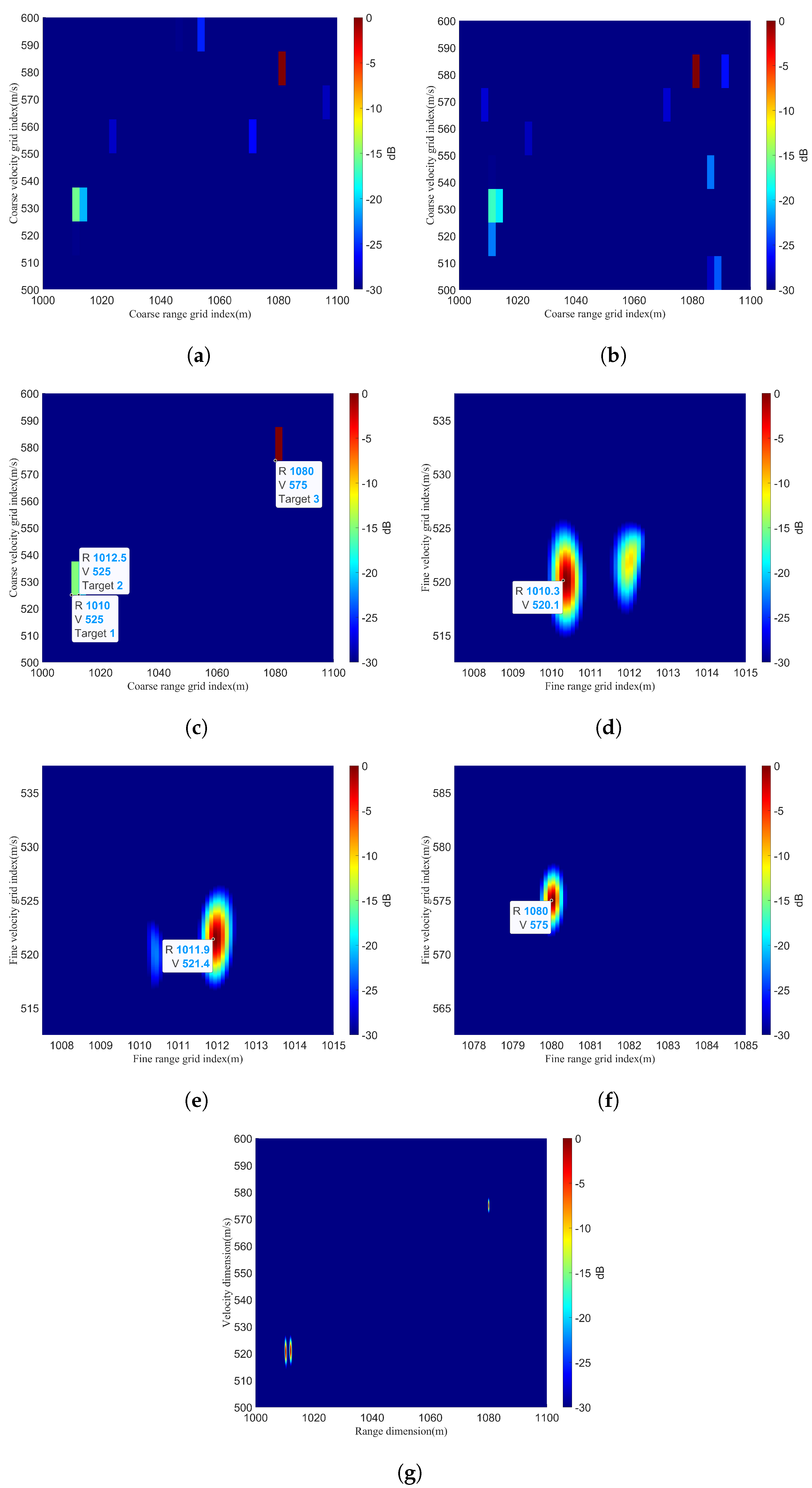
In Table 5, it is evident that in Scenario 1, the proposed algorithm exhibits comparable performance to other algorithms in addressing off−grid issues. This can be attributed to the fact that Scenario 1 is relatively simplistic in comparison to other scenarios, which might not fully reflect the distinctive characteristics of each algorithm. In the context of multiple targets, the proposed algorithm outperforms other algorithms in Scenario 2 and Scenario 3. It is worth noting that as the targets transition from non-neighboring to close in both range and velocity, the RMSE of each algorithm exhibits an increasing trend, indicating that closely spaced targets severely impact the performance. It can also be observed that the proposed algorithm is less affected in this case due to the use of the SBL framework with the GDP distribution. It is noted that although the performance of the GI−MSBL algorithm is inferior to that of the proposed RGDP−SBL algorithm, it is superior to other algorithms. Consequently, a detailed comparison of the specific simulation results between the GI−MSBL algorithm and the proposed RGDP−SBL algorithm is also undertaken. During the simulation, it was observed that the entire range−velocity plane exhibited multiple high-energy false targets in the simulation result of the coarse search, which could potentially affect the identification of the true target. However, the positions of these false targets on the range−velocity plane are random. Therefore, by employing a method of multiple detections, the randomly positioned false targets could be disregarded, retaining only the true targets that have a fixed position on the range−velocity plane. The method of multiple detections involves conducting three coarse searches, retaining targets that appear at least twice at the same location, and discarding targets that emerge randomly. The specific simulation results of the GI−MSBL algorithm and RGDP−SBL algorithm in Scenario 1, Scenario 2, and Scenario 3 are shown in Figure 6, Figure 7, Figure 8, Figure 9, Figure 10 and Figure 11. In each set of figures, the results include the coarse search results from two detections, the coarse search results after multiple detections, the results of the local fine search, and the overall effect on the range−velocity plane.
From these figures, it can be observed that the proposed RGDP−SBL algorithm achieves accurate signal recovery for targets precisely located on grid points, therefore obtaining precise range and velocity information of the targets. Meanwhile, the proposed algorithm attains high-precision target parameter estimation for targets under off−grid conditions, surpassing the performance of algorithms based on on−grid assumptions, therefore achieving a superior level of performance. Therefore, the proposed RGDP−SBL algorithm can accurately obtain the range and velocity information of targets in these scenarios. Moreover, the GI−MSBL algorithm produces more false targets in each scenario compared to the proposed RGDP−SBL algorithm, therefore increasing the probability of false alarms for single detection. Additionally, it is clearly observable that in each scenario, there is a significant difference in the fine search results of these two algorithms. The fine search results of the proposed RGDP−SBL algorithm exhibit a narrower main lobe with smaller sidelobes and more concentrated energy. In contrast, the fine search results of the GI−MSBL algorithm show a broader main lobe with numerous sidelobes around it, leading to a more dispersed energy distribution. This may be attributed to the stronger sparsity of the GDP distribution utilized in the RGDP−SBL algorithm. Therefore, the proposed algorithm demonstrates higher accuracy and more effective sidelobe suppression compared to the GI−MSBL algorithm.

3.4.2. Impact of Performance Due to Different SNR Values

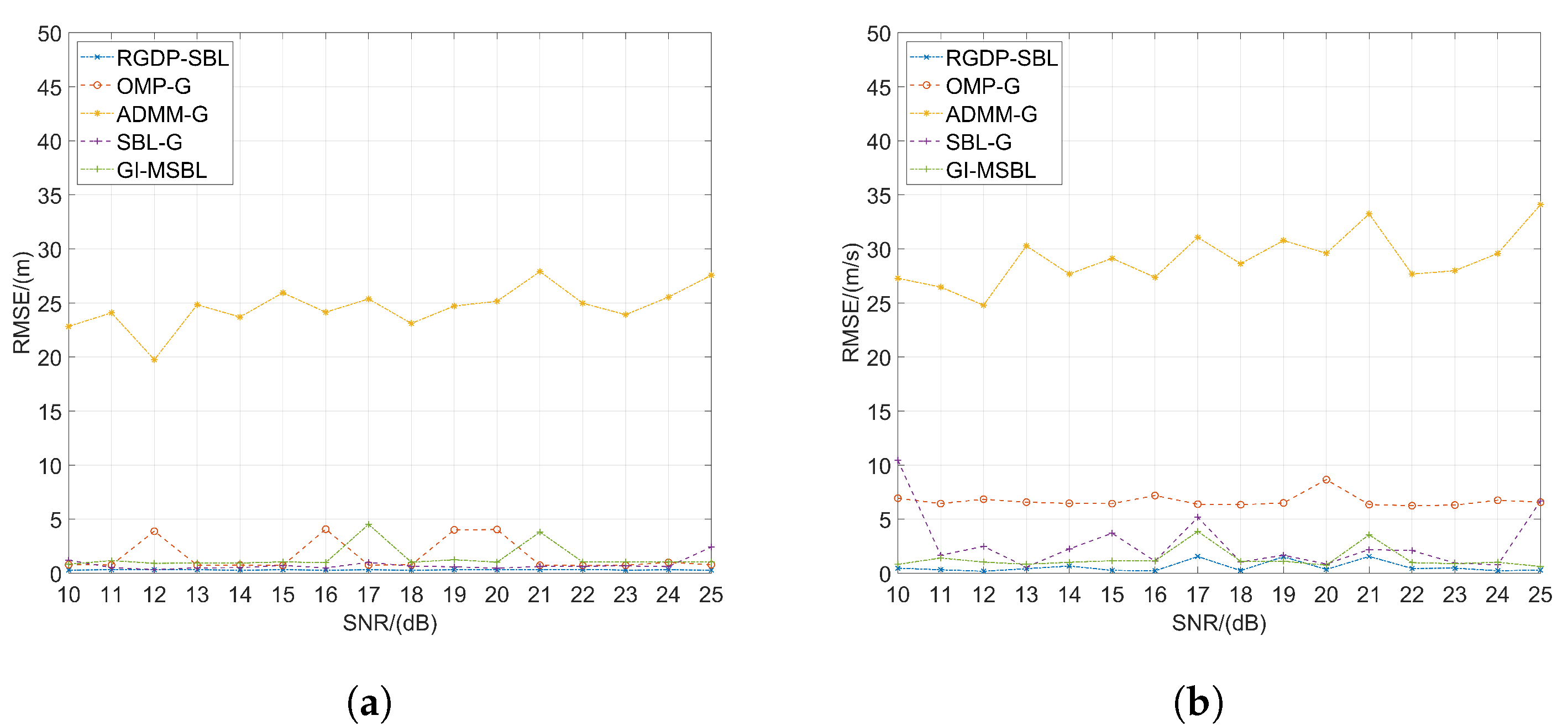
To assess the robustness of each algorithm under different SNR conditions and their capability to detect weak targets in scenarios involving closely spaced targets, based on the range and velocity parameters of the targets in Scenario 3, the SNR of Target 1 and Target 2 is varied from 10 to 25. Simultaneously, the SNR of Target 3, which is accurately located on the range−velocity grid points, is kept constant at 30, ensuring its consistent status as a strong target. The results averaged over 200 independent Monte Carlo simulations for each SNR level are given in Figure 12.
As illustrated, the proposed RGDP−SBL algorithm achieves the best performance compared with other algorithms in all SNR levels. Particularly in Scenario 3, the increased correlation between columns of the observation matrix has severely affected the performance of OMP−G and ADMM−G algorithms, resulting in larger RMSE values for range and velocity in ADMM−G, as well as a larger RMSE for velocity in OMP−G. Simultaneously, the performance of the GI−MSBL algorithm is not stable, as it demonstrates relatively large RMSE values under certain SNR conditions. In contrast, the proposed algorithms and SBL-G are successful in consistently maintaining lower RMSE values for both velocity and range, but the RMSE of SBL−G is still larger than that of the proposed algorithms. This can be attributed to the fact that the proposed algorithm effectively mitigates the impact of various factors on parameter estimation by utilizing the high sparsity of the GDP distribution and implementing two rounds of hyperparameter updates during the fine search process. For this reason, the proposed algorithm demonstrates superior noise resilience compared to other algorithms.

3.4.3. Impact of Performance Due to Different Target Numbers

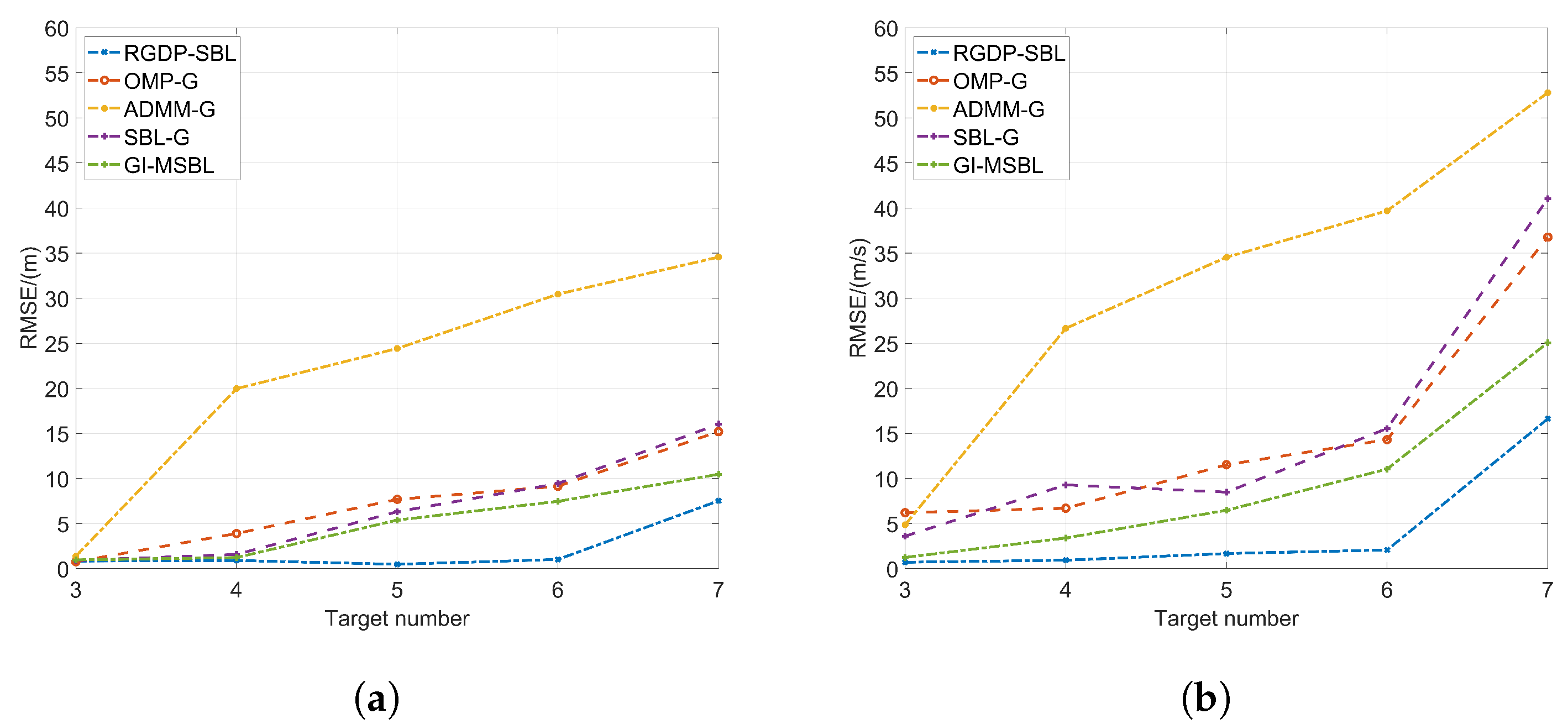
In addition to noise, it is also essential to investigate the impact of different numbers of targets on performance. Therefore, the simulation is carried out under scenarios from Scenario 3 to Scenario 7, where the range of target numbers varies from 3 to 7. For each number of targets, results are obtained by averaging over 200 independent Monte Carlo simulations. The simulation results are shown in the Figure 13.
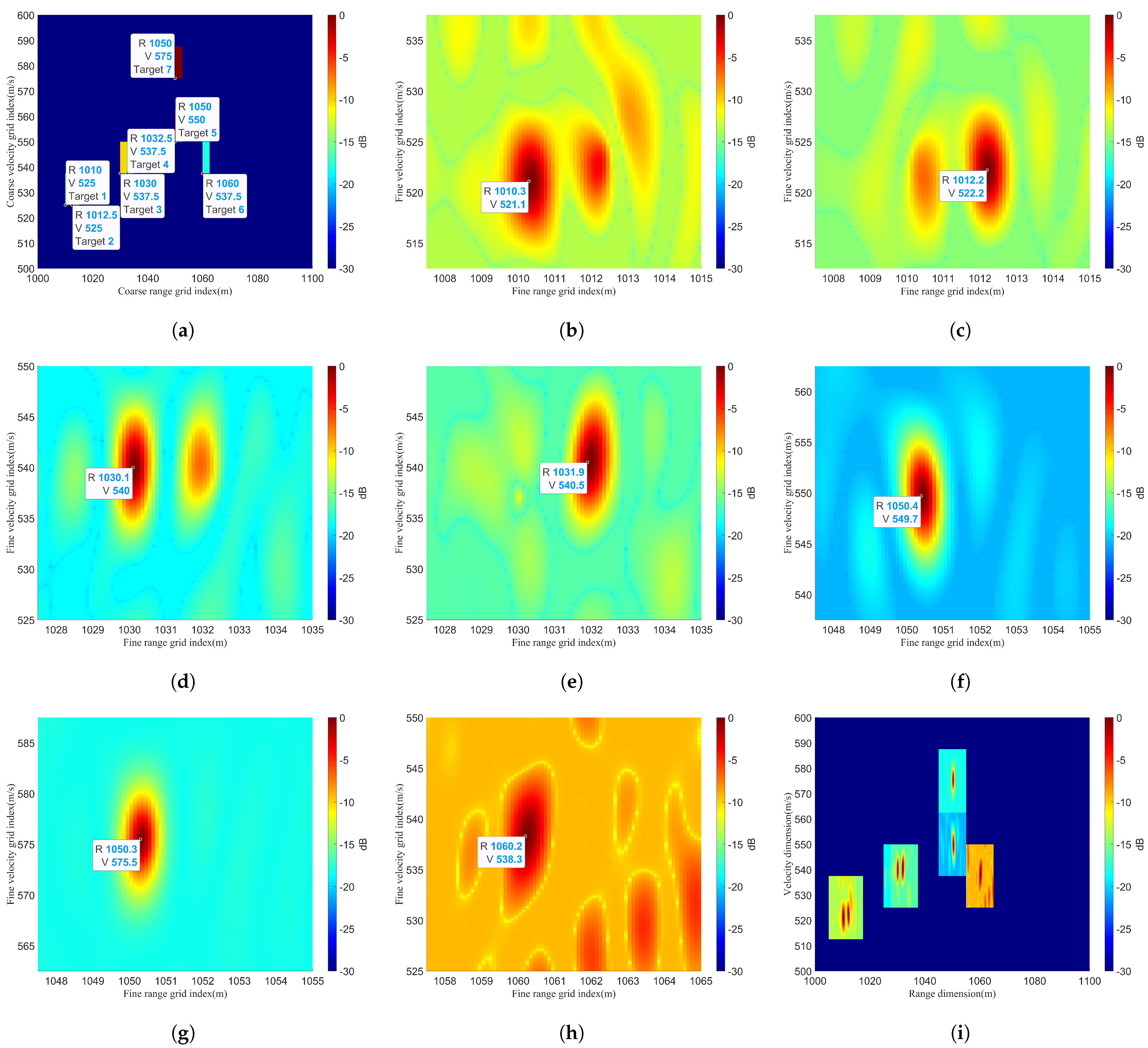
As shown in Figure 13, the performance of all four algorithms demonstrates a declining trend as the number of targets increases. This is mainly because an increasing number of targets leads to reduced sparsity in the radar echoes, consequently affecting the recovery performance. Importantly, the proposed algorithm demonstrates a relatively low sensitivity to off−grid issues and the number of targets, therefore maintaining a reduced RMSE compared to the other three algorithms. However, when the number of targets increases to 7, the performance of the proposed algorithm experiences a substantial deterioration. The specific simulation results of the proposed RGDP−SBL algorithm in Scenario 7 with 7 targets are illustrated in Figure 14.
As depicted in Figure 14, in Scenario 7, the proposed algorithm exhibited limitations in accurately extracting the range−velocity information for Target 6 and Target 7, leading to considerable errors. Consequently, there exists a significant scope for enhancing the performance of the proposed algorithm.

4. Discussion

4.1. Discussion of Computational Complexity

The proposed RGDP−SBL algorithm assumes that the original signal follows a complex GDP prior distribution, significantly increasing computational complexity. Therefore, methods to reduce computational complexity are considered in both the coarse and fine search parts. In Section 2.3, during the derivation of the coarse search part of the proposed algorithm, it can be observed that only the diagonal elements of the posterior variance Σ are utilized, therefore eliminating the need to compute the entire matrix, as compared to the SBL algorithm in [22]. For the SBL algorithm in [22], the computational complexity mainly originates from the calculation of Φ H Σ y 1 Φ , thus the total computational complexity is given by O ( J N 2 + J 2 N ) . The computational complexity required for the Σ j j computation primarily comes from the value of ( Φ H Σ y 1 ) j Φ j in the proposed algorithm, and the total computational complexity is given by O ( J N 2 + J N ) . The computational complexity of the RGDP−SBL algorithm for RFPA radar is evaluated specifically for the coarse search part since the off−grid scenarios are not considered in [22]. In the on−grid simulation case, 200 Monte Carlo simulations are conducted for each algorithm to obtain average run times, facilitating comparative analysis. The average running time is shown in Table 6.
Furthermore, during the fine search, the grid energy amplitude curve can be approximated as a convex curve with a turning point, which corresponds precisely to the grid point required by the algorithm during the fine search process. This grid point can be converted to range−velocity coordinates, enabling the parameters of the target to be obtained without calculating the values of the grid energy, therefore reducing computational complexity. Consequently, the use of methods to reduce computational complexity during both the coarse and fine search processes can offset the increase in computational complexity caused by the GDP distribution, as mentioned in Section 2.2.

4.2. Discussion of Performance

In previous studies, sparse reconstruction algorithms based on CS for RFPA radar typically assume that targets are accurately positioned on range−velocity grid points. However, this assumption can introduce substantial errors in scenarios where targets are off−grid. Simultaneously, CS algorithms that employ the SBL method with simple model priors also experience a decrease in the performance of target range and velocity parameter estimation due to inadequate sparsity.
Therefore, to mitigate the impact of the off−grid problem, the proposed algorithm is principally divided into two parts: coarse and fine searches. Moreover, the algorithm employs the GDP distribution, which has stronger sparsity, to enhance the performance of range and velocity parameter estimation. Under the on−grid assumption, the proposed algorithm outperforms the SBL, ADMM, OMP, and GI−MSBL algorithms due to its utilization of the more sparsely intense GDP distribution. Additionally, under the off−grid assumption, the performance of the proposed algorithm surpasses the other four algorithms. In the fine search process, due to the secondary update of hyperparameters based on the GDP distribution, the proposed algorithm achieves greater performance of sidelobe suppression and higher precision compared to the GI−MSBL algorithm. Furthermore, under varying SNR and different numbers of targets, the performance of the proposed algorithm also outperforms the other four algorithms. Current research employs off−grid CS algorithms based on SBL for the estimation of range−angle−velocity parameters. Consequently, with the implementation of appropriate algorithmic modifications, the proposed algorithm should be applicable within this field.

5. Conclusions

To enhance signal recovery performance and mitigate the impact of off−grid issues on target parameter estimation for RFPA radar, this paper proposes an off−grid CS algorithm named RGDP−SBL, which synergistically combines the SBL−based algorithm with grid refinement. Specifically, the algorithm posits a GDP prior distribution for the original signal and incorporates a two-stage coarse-fine search within the SBL framework. Through comprehensive simulations, the performance of the proposed RGDP-SBL algorithm is compared with other CS algorithms in terms of on−grid cases and off−grid cases. In this study, the frequency agility range of the RFPA radar is observed to be relatively limited, and the performance of the proposed algorithm significantly deteriorates when dealing with many targets. Therefore, future research will emphasize improvements in both aspects. Furthermore, we plan to adapt and innovate this algorithm for low-angle tracking in future research, therefore facilitating the accurate estimation of distance-angle-velocity parameters.

Author Contributions

Conceptualization, J.W.; methodology, B.S. and Y.Z. (Yi Zhao); software, B.S. and Y.Z. (Yi Zhao); writing—original draft preparation, B.S. and S.D.; writing—review and editing, J.W and Y.Z. (Yi Zhong); supervision, J.W.; funding acquisition, J.W. All authors have read and agreed to the published version of the manuscript.

Funding

This research was funded by the National Natural Science Foundation of China (grant number 61971043).

Data Availability Statement

The data are available from the corresponding author on reasonable request. The data are not publicly available due to that there are still graduate students using it for research.

Conflicts of Interest

The authors declare no conflict of interest.

Abbreviations

The following abbreviations are used in this manuscript:
PRIPulse Repetition Interval
RFPARandom Frequency and Pulse Repetition Interval Agile
CSCompressed Sensing
SBLSparse Bayesian Learning
BPBasis Pursuit
ADMMAlternating Direction Method of Multipliers
NPNondeterministic Polynomial
OMPOrthogonal Matching Pursuit
DOADirection of Arrive
MIMOMultiple−Input Multiple−Output
CS−IGOCS−Iterative Grid Optimization
AMP−CTLSAdaptive Matching Pursuit with Constrained Total Least Squares
PSOParticle Swarm Optimization
OGSBIOff−Grid Sparse Bayesian Inference
GI−MSBLGrid Interpolation-Multiple snapshot SBL
GDPGeneralized Double Pareto
RGDP−SBLgrid Refinement and GDP distribution based on SBL
CPICoherent Processing Interval
PDFProbability Density Function
EMExpectation-Maximization
E−stepExpectation step
M−stepMaximization step
RMSERoot Mean Square Error
SNRsignal−to−noise ratio

References

  1. Long, X.W.; Li, K.; Tian, J.; Wang, J.; Wu, S.L. Ambiguity Function Analysis of Random Frequency and PRI Agile Signals. IEEE Trans. Aerosp. Electron. Syst. 2021, 57, 382–396. [Google Scholar] [CrossRef]
  2. Quan, Y.H.; Fang, W.; Gao, X.; Ruan, F.; Li, Y.C.; Xing, M.D. Review on Frequency Agile Radar Seeker. Aero Weapon. 2021, 28, 1–9. (In Chinese) [Google Scholar]
  3. Pace, P.E. Detecting and Classifying Low Probability of Intercept Radar, 2nd ed.; Artech: Morristown, NJ, USA, 2008. [Google Scholar]
  4. Blunt, S.D.; Mokole, E.L. Overview of radar waveform diversity. IEEE Aerosp. Electron. Syst. Mag. 2016, 31, 2–42. [Google Scholar] [CrossRef]
  5. Long, X.W.; Wu, W.H.; Li, K.; Wang, J.; Wu, S.L. Multi-Timeslot Wide-Gap Frequency-Hopping RFPA Signal and Its Sidelobe Suppression. IEEE Trans. Aerosp. Electron. Syst. 2023, 59, 634–649. [Google Scholar] [CrossRef]
  6. Axelsson, S.R.J. Analysis of Random Step Frequency Radar and Comparison With Experiments. IEEE Trans. Geosci. Remote Sens. 2007, 45, 890–904. [Google Scholar] [CrossRef]
  7. Kulpa, J.S. Noise radar sidelobe suppression algorithm using mismatched filter approach. Int. J. Microw. Wirel. Technol. 2016, 8, 865–869. [Google Scholar] [CrossRef]
  8. Costas, J.P. A study of a class of detection waveforms having nearly ideal range-Doppler ambiguity properties. Proc. IEEE 1984, 72, 996–1009. [Google Scholar] [CrossRef]
  9. Maric, S.; Titlebaum, E.L. A class of frequency hop codes with nearly ideal characteristics for use in multiple-access spread-spectrum communications and radar and sonar systems. IEEE Trans. Commun. 1992, 40, 1442–1447. [Google Scholar] [CrossRef]
  10. Donoho, D.L. Compressed sensing. IEEE Trans. Inf. Theory 2006, 52, 1289–1306. [Google Scholar] [CrossRef]
  11. Huang, T.Y. Coherent Frequency-Agile Radar Signal Processing by Solving an Inverse Problem with a Sparsity Constraint. Ph.D. Thesis, Tsinghua University, Beijing, China, 2014. [Google Scholar]
  12. Anitori, L.; Maleki, A.; Otten, M.; Baraniuk, R.G.; Hoogeboom, P. Design and Analysis of Compressed Sensing Radar Detectors. IEEE Trans. Signal Process. 2013, 61, 813–827. [Google Scholar] [CrossRef]
  13. Quan, Y.H.; Fang, W.; Sha, M.H.; Chen, X.D.; Ruan, F.; Li, X.H.; Meng, F.; Wu, Y.J.; Xing, M.D. Present situation and prospects of frequency agility radar waveform countermeasures. Syst. Eng. Electron. 2021, 43, 3126–3136. [Google Scholar]
  14. Yang, J.G. Research on Sparsity-Driven Regularization Radar Imaging Theory and Method. Ph.D. Thesis, National University of Defense Technology, Changsha, China, 2013. [Google Scholar]
  15. Boyd, S.; Parikh, N.; Chu, E.; Peleato, B.; Eckstein, J. Distributed Optimization and Statistical Learning via the Alternating Direction Method of Multipliers. Found. Trends® Mach. Learn. 2011, 3, 1–122. [Google Scholar]
  16. Liu, Z.; Wei, X.Z.; Li, X. Low sidelobe robust imaging in random frequency-hopping wideband radar based on compressed sensing. J. Cent. South Univ. 2013, 20, 702–714. [Google Scholar] [CrossRef]
  17. Wang, W. A Study of Convex Relaxation Algorithms for Compressed Sensing Reconstruction Problem. Master’s Dissertation, Xidian University, Xi’an, China, 2014. [Google Scholar]
  18. Huang, T.Y.; Liu, Y.M.; Xu, X.Y.; Xu, X.Y.; Eldar, Y.C.; Wang, X.Q. Analysis of Frequency Agile Radar via Compressed Sensing. IEEE Trans. Signal Process. 2018, 66, 6228–6240. [Google Scholar] [CrossRef]
  19. Quan, Y.H.; Wu, Y.J.; Li, Y.C.; Sun, G.C.; Xing, M.D. Range-Doppler reconstruction for frequency agile and PRF-jittering radar. IET Radar, Sonar Navig 2017, 12, 348–352. [Google Scholar] [CrossRef]
  20. Wipf, D.; Palmer, J.; Rao, B. Perspectives on Sparse Bayesian Learning. Adv. Neural Inf. Process. Syst. 2003, 16, 249–256. [Google Scholar]
  21. Wipf, D.; Rao, B. Sparse Bayesian Learning for Basis Selection. IEEE Trans. Signal Process. 2004, 52, 2153–2164. [Google Scholar] [CrossRef]
  22. Tao, Y.J.; Zhang, G.; Tao, T.B.; Leng, Y.; Leung, H. Frequency-agile Coherent Radar Target Sidelobe Suppression Based on Sparse Bayesian Learning. In Proceedings of the 2019 IEEE MTT-S International Microwave Biomedical Conference (IMBioC), Nanjing, China, 6–8 May 2019; Volume 1, pp. 1–4. [Google Scholar]
  23. Tipping, M.E. Sparse Bayesian learning and the relevance vector machine. J. Mach. Learn. Res. 2001, 1, 211–244. [Google Scholar]
  24. Huang, Q.H.; Zhang, G.F.; Fang, Y. Real-valued DOA estimation for spherical arrays using sparse Bayesian learning. Signal Process. 2016, 125, 79–86. [Google Scholar] [CrossRef]
  25. Liu, H.C.; Jiu, B.; Liu, H.W.; Bao, Z. A novel ISAR imaging algorithm for micromotion targets based on multiple sparse Bayesian learning. IEEE Geosci. Remote Sens. Lett. 2014, 11, 1772–1776. [Google Scholar]
  26. Liu, Z.X.; Zhu, S.Q.; Xu, J.W.; Lan, L. An Adaptive Range-Angle-Doppler Processing Approach for FDA-MIMO Radar Based on Sparse Reconstruction. In Proceedings of the 2021 CIE International Conference on Radar (Radar), Haikou, China, 15–19 December 2021; pp. 1704–1708. [Google Scholar]
  27. Wipf, D. Sparse estimation with structured dictionaries. Adv. Neural Inf. Process. Syst. 2011, 24, 2016–2024. [Google Scholar]
  28. Chae, D.H.; Sadeghi, P.; Kennedy, R.A. Effects of basis-mismatch in compressive sampling of continuous sinusoidal signals. In Proceedings of the 2010 2nd International Conference on Future Computer and Communication, Wuhan, China, 21–24 May 2010; Volume 2, pp. V2-739–V2-743. [Google Scholar]
  29. Chi, Y.J.; Scharf, L.L.; Pezeshki, A.; Calderbank, A.R. Sensitivity to Basis Mismatch in Compressed Sensing. IEEE Trans. Signal Process. 2011, 59, 2182–2195. [Google Scholar] [CrossRef]
  30. Liu, Z.; Wei, X.Z.; Li, X. Adaptive clutter suppression for airborne random pulse repetition interval radar based on compressed sensing. Prog. Electromagn. Res. 2012, 128, 291–311. [Google Scholar] [CrossRef]
  31. Huang, T.Y.; Liu, Y.M.; Meng, H.D.; Wang, X.Q. Adaptive Matching Pursuit for Off-Grid Compressed Sensing. arXiv 2013, arXiv:arXiv:13084273. [Google Scholar]
  32. Chen, Q.; Wu, X.J.; Liu, J.H. Adaptive compressed sensing based randomized step frequency radar with a weighted PSO. In Proceedings of the 2015 IEEE International Conference on Information and Automation, Lijiang, China, 8–10 August 2015; pp. 1751–1756. [Google Scholar]
  33. Zhang, G.B.; Huang, T.Y.; Liu, Y.M.; Eldar, Y.C.; Wang, X.Q. Frequency Agile Radar Using Atomic Norm Soft Thresholding with Modulations. In Proceedings of the 2019 IEEE Radar Conference (RadarConf), Boston, MA, USA, 22–26 April 2019; pp. 1–6. [Google Scholar]
  34. Yang, Z.; Xie, L.H.; Zhang, C.S. Off-Grid Direction of Arrival Estimation Using Sparse Bayesian Inference. IEEE Trans. Signal Process. 2013, 61, 38–43. [Google Scholar] [CrossRef]
  35. Dai, J.S.; Bao, X.; Xu, W.C.; Chang, C.Q. Root Sparse Bayesian Learning for Off-Grid DOA Estimation. IEEE Signal Process. Lett. 2017, 24, 46–50. [Google Scholar] [CrossRef]
  36. Wang, Q.S.; Yu, H.; Li, J.; Dong, C.; Ji, F.; Chen, Y.K. Sparse Bayesian Learning Based Algorithm for DOA Estimation of Closely Spaced Signals. J. Electron. Inf. Technol. 2021, 43, 708–716. [Google Scholar]
  37. Wipf, D.P. Bayesian Methods for Finding Sparse Representations; University of California: San Diego, CA, USA, 2006. [Google Scholar]
  38. Huang, T.Y.; Liu, Y.M.; Meng, H.D.; Wang, X.Q. Adaptive waveform design in random stepped frequency radar. In Proceedings of the IET International Radar Conference 2013, Xi’an, China, 14–16 April 2013; pp. 1–5. [Google Scholar]
  39. Gerstoft, P.; Mecklenbräuker, C.F.; Xenaki, A.; Nannuru, S. Multisnapshot Sparse Bayesian Learning for DOA. IEEE Signal Process. Lett. 2016, 23, 1469–1473. [Google Scholar] [CrossRef]
  40. Ji, S.H.; Xue, Y.; Carin, L. Bayesian Compressive Sensing. IEEE Trans. Signal Process. 2008, 56, 2346–2356. [Google Scholar] [CrossRef]
  41. Armagan, A.; Dunson, D.B.; Lee, J. Generalized double Pareto shrinkage. Stat. Sin. 2011, 23, 119–143. [Google Scholar] [CrossRef]
  42. Wang, Q.S.; Yu, H.; Li, J.; Ji, F.; Chen, F.J. Sparse Bayesian Learning Using Generalized Double Pareto Prior for DOA Estimation. IEEE Signal Process. Lett. 2021, 28, 1744–1748. [Google Scholar] [CrossRef]
  43. Wipf, D.; Rao, B. An Empirical Bayesian Strategy for Solving the Simultaneous Sparse Approximation Problem. IEEE Trans. Signal Process. 2007, 55, 3704–3716. [Google Scholar] [CrossRef]
  44. Giri, R.; Rao, B. Type I and Type II Bayesian Methods for Sparse Signal Recovery Using Scale Mixtures. IEEE Trans. Signal Process. 2016, 64, 3418–3428. [Google Scholar] [CrossRef]
  45. Dempster, A.P.; Laird, N.M.; Rubin, D. Maximum Likelihood from Incomplete Data Via the EM Algorithm. J. R. Stat. Soc. Ser. B (Methodol.) 1977, 39, 1–22. [Google Scholar] [CrossRef]
  46. Wang, A.P.; Zhang, G.Y.; Liu, F. Research and Application of EM Algorithm. Comput. Technol. Dev. 2009, 19, 108–110. (In Chinese) [Google Scholar]
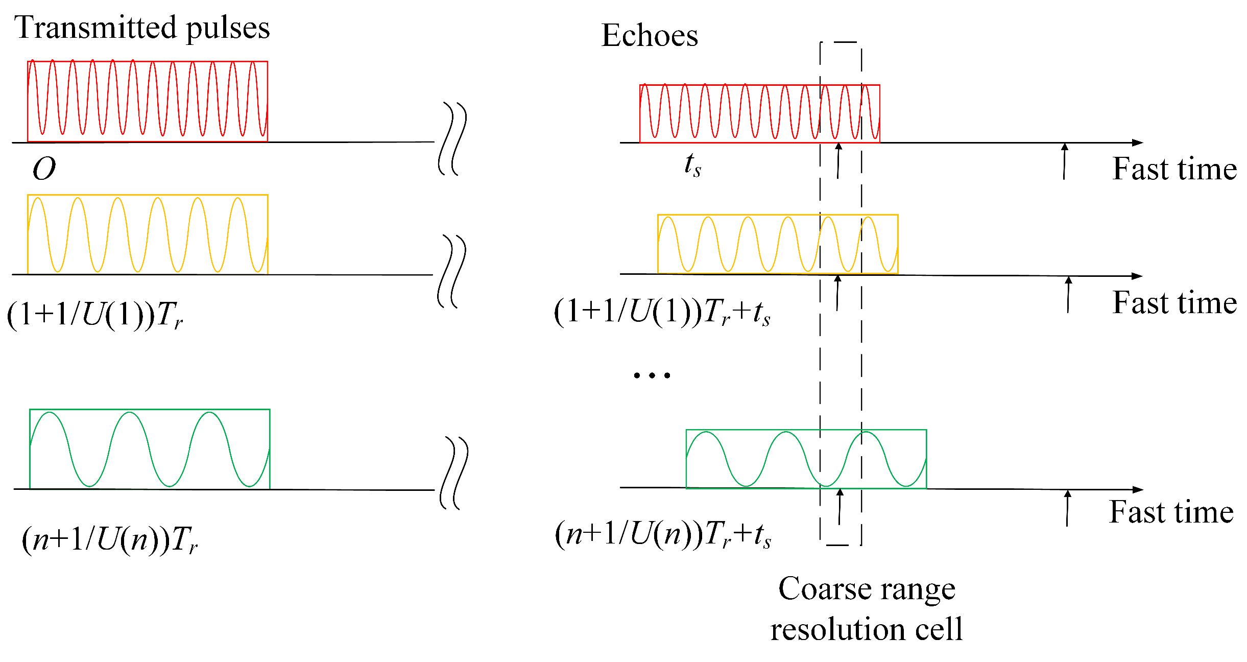
Figure 1. Process of acquiring observation data.
Remotesensing 16 00403 g001
Figure 2. The signal observation model based on CS.
Remotesensing 16 00403 g002
Figure 3. The real positions of the targets in Scenario 2.
Remotesensing 16 00403 g003
Figure 4. The real positions of the targets in Scenario 7.
Remotesensing 16 00403 g004
Figure 5. Impact on performance due to δ variations in Scenario 3: (a) Range RMSE. (b) Velocity RMSE.
Remotesensing 16 00403 g005
Figure 6. Simulation results of the GI−MSBL algorithm in Scenario 1: (a) The coarse search result of the first detection. (b) The coarse search result of the second detection. (c) The coarse search result after multiple detections. (d) Result of the local fine search. (e) The overall effect on the range−velocity plane.
Remotesensing 16 00403 g006
Figure 7. Simulation results of the RGDP−SBL algorithm in Scenario 1: (a) The coarse search result of the first detection. (b) The coarse search result of the second detection. (c) The coarse search result after multiple detections. (d) Result of the local fine search. (e) The overall effect on the range−velocity plane.
Remotesensing 16 00403 g007
Figure 8. Simulation results of the GI−MSBL algorithm in Scenario 2: (a) The coarse search result of the first detection. (b) The coarse search result of the second detection. (c) The coarse search result after multiple detections. (d) Result of the local fine search for Target 1. (e) Result of the local fine search for Target 2. (f) Result of the local fine search for Target 3. (g) The overall effect on the range−velocity plane.
Remotesensing 16 00403 g008
Figure 9. Simulation results of the RGDP−SBL algorithm in Scenario 2: (a) The coarse search result of the first detection. (b) The coarse search result of the second detection. (c) The coarse search result after multiple detections. (d) Result of the local fine search for Target 1. (e) Result of the local fine search for Target 2. (f) Result of the local fine search for Target 3. (g) The overall effect on the range−velocity plane.
Remotesensing 16 00403 g009
Figure 10. Simulation results of the GI−MSBL algorithm in Scenario 3: (a) The coarse search result of the first detection. (b) The coarse search result of the second detection. (c) The coarse search result after multiple detections. (d) Result of the local fine search for Target 1. (e) Result of the local fine search for Target 2. (f) Result of the local fine search for Target 3. (g) The overall effect on the range−velocity plane.
Remotesensing 16 00403 g010
Figure 11. Simulation results of the RGDP−SBL algorithm in Scenario 3: (a) The coarse search result of the first detection. (b) The coarse search result of the second detection. (c) The coarse search result after multiple detections. (d) Result of the local fine search for Target 1. (e) Result of the local fine search for Target 2. (f) Result of the local fine search for Target 3. (g) The overall effect on the range−velocity plane.
Remotesensing 16 00403 g011
Figure 12. Impact on performance due to SNR variations in Scenario 3: (a) Range RMSE. (b) Velocity RMSE.
Remotesensing 16 00403 g012
Figure 13. Impact on performance due to target number variations in Scenario 3: (a) Range RMSE. (b) Velocity RMSE.
Remotesensing 16 00403 g013
Figure 14. Simulation results of the RGDP−SBL algorithm in Scenario 7: (a) Result of the coarse search. (b) Result of the local fine search for Target 1. (c) Result of the local fine search for Target 2. (d) Result of the local fine search for Target 3. (e) Result of the local fine search for Target 4. (f) Result of the local fine search for Target 5. (g) Result of the local fine search for Target 6. (h) Result of the local fine search for Target 7. (i) The overall effect on the range−velocity plane.
Remotesensing 16 00403 g014
Table 1. Simulation parameters for RFPA radar.
ParametersSymbolsValuesUnits
Central Carrier Frequency f c 10GHz
Average PRI T r 10 μ s
Pulse Width T w 1 μ s
Bandwidth of Frequency−Hopping Step Δ f 1MHz
Pulse NumberN128-
Frequency agility rangeB128MHz
PRI agility range T n 5 μ s
Table 2. Parameter settings for scenarios.
ScenariosTargetsRange (m)Velocity (m/s)SNR (dB)
Scenario 1Target 11011.57521.320
Scenario 2Target 11011.57521.320
Target 21051.7551.0620
Target 3108057530
Scenario 3Target 11011.57521.320
Target 21010.7520.0620
Target 3108057530
Scenario 4Target 11011.57521.320
Target 21010.7520.0620
Target 31030.1540.7620
Target 4108057530
Scenario 5Target 11011.57521.320
Target 21010.7520.0620
Target 31030.1540.7620
Target 41031.7541.0620
Target 5108057530
Scenario 6Target 11011.57521.320
Target 21010.7520.0620
Target 31030.1540.7620
Target 41031.7541.0620
Target 51050.7550.120
Target 6108057530
Scenario 7Target 11011.57521.320
Target 21010.7520.0620
Target 31030.1540.7620
Target 41031.7541.0620
Target 51050.7550.120
Target 61050.3551.420
Target 7108057530
Table 3. Impact on performance due to scenario variations.
ScenariosDistribution R RMSE (m) V RMSE (m/s)
Scenario 1complex Gaussian0.933.70
Laplace0.933.70
GDP0.673.70
Scenario 2complex Gaussian1.092.72
Laplace0.722.70
GDP0.702.22
Scenario 3complex Gaussian2.514.01
Laplace0.903.85
GDP0.723.97
Table 4. Impact on performance due to scenario variations.
ScenariosAlgorithms R RMSE (m) V RMSE (m/s)
Scenario 1OMP−C0.816.10
ADMM0.766.10
SBL0.933.70
GI−MSBL−C0.933.70
RGDP−SBL−C0.673.70
Scenario 2OMP−C0.712.11
ADMM0.712.31
SBL1.012.22
GI−MSBL−C0.712.22
RGDP−SBL−C0.702.22
Scenario 3OMP−C1.383.78
ADMM0.995.82
SBL2.514.18
GI−MSBL−C0.713.85
RGDP−SBL−C0.673.56
Table 5. Impact on performance due to scenario variations.
ScenariosAlgorithms R RMSE (m) V RMSE (m/s)
Scenario 1OMP−G *0.570.70
ADMM−G *0.420.66
SBL−G *0.050.45
GI−MSBL−G *0.030.10
RGDP−SBL **0.030.06
Scenario 2OMP−G *0.451.89
ADMM−G *0.712.23
SBL−G *0.460.71
GI−MSBL−G *0.110.23
RGDP−SBL **0.040.14
Scenario 3OMP−G *1.373.56
ADMM−G *0.974.85
SBL−G *1.373.56
GI−MSBL−G *1.021.13
RGDP−SBL **0.410.96
* “−G” refers to the use of combining with grid refinement algorithm. ** “RGDP−SBL” refers to the proposed algorithm with the fine search part.
Table 6. The average running time of different algorithms.
AlgorithmsTarget ScenariosRunning Time (s)Computational Complexity
SBL * in [22]Scenario 10.43058 O ( J N 2 + J 2 N )
Scenario 20.62564
Scenario 31.25592
RGDP−SBL−C **Scenario 10.0887 O ( J N 2 + J N )
Scenario 20.11848
Scenario 30.1267
* “SBL” refers to the algorithm in [22]. ** “RGDP−SBL−C” refers to the RGDP−SBL with only coarse search part.
Disclaimer/Publisher’s Note: The statements, opinions and data contained in all publications are solely those of the individual author(s) and contributor(s) and not of MDPI and/or the editor(s). MDPI and/or the editor(s) disclaim responsibility for any injury to people or property resulting from any ideas, methods, instructions or products referred to in the content.