
A Spatial–Spectral Transformer for Hyperspectral Image Classification Based on Global Dependencies of Multi-Scale Features


Abstract
1. Introduction
- 1.
- To tackle the challenge of the transformer inadequately leveraging spatial–spectral features, we redesigned the feature extractor—SSTG. SSTG incorporates a dense multi-dimensional convolutional structure, adeptly extracting HSI spatial–spectral features. Additionally, it introduces a branch to extract spectral features of query pixels, compensating for damaged spectral features during the convolution process. Attention encoding on features from SSTG enables the expression of spatial–spectral semantic characteristics of HSI during classification.
- 2.
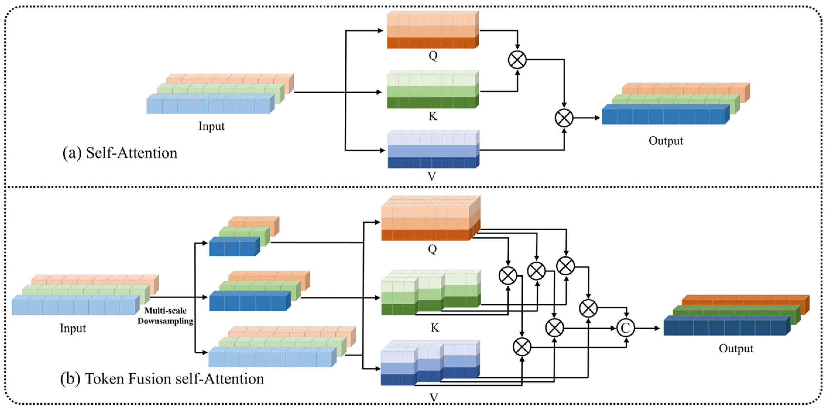
- To simulate global dependencies among multi-scale features during attention modeling, we innovatively introduce TFSA. This module, after subsampling tokens to varying extents, generates keys and values of different sizes. Subsequently, different attention heads compute attention outputs by operating on the corresponding-sized keys, values, and queries. This novel attention mechanism effectively simulates global dependencies among multi-scale features, demonstrating enhanced capabilities in classifying multi-scale targets.
- 3.
- We employed SSTG and TFSA, introducing CCA to construct the MSST HSI classification network. This hybrid network effectively integrates both global and local modeling capabilities, enabling the consideration of multi-scale characteristics of targets in HSI and the effective utilization of spatial–spectral features.
2. Related Research
2.1. Applying Spatial–Spectral Information to Transformer
2.2. Multi-Scale Attention Modeling in Transformer
3. Methods
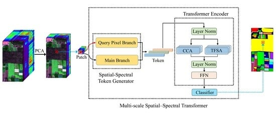
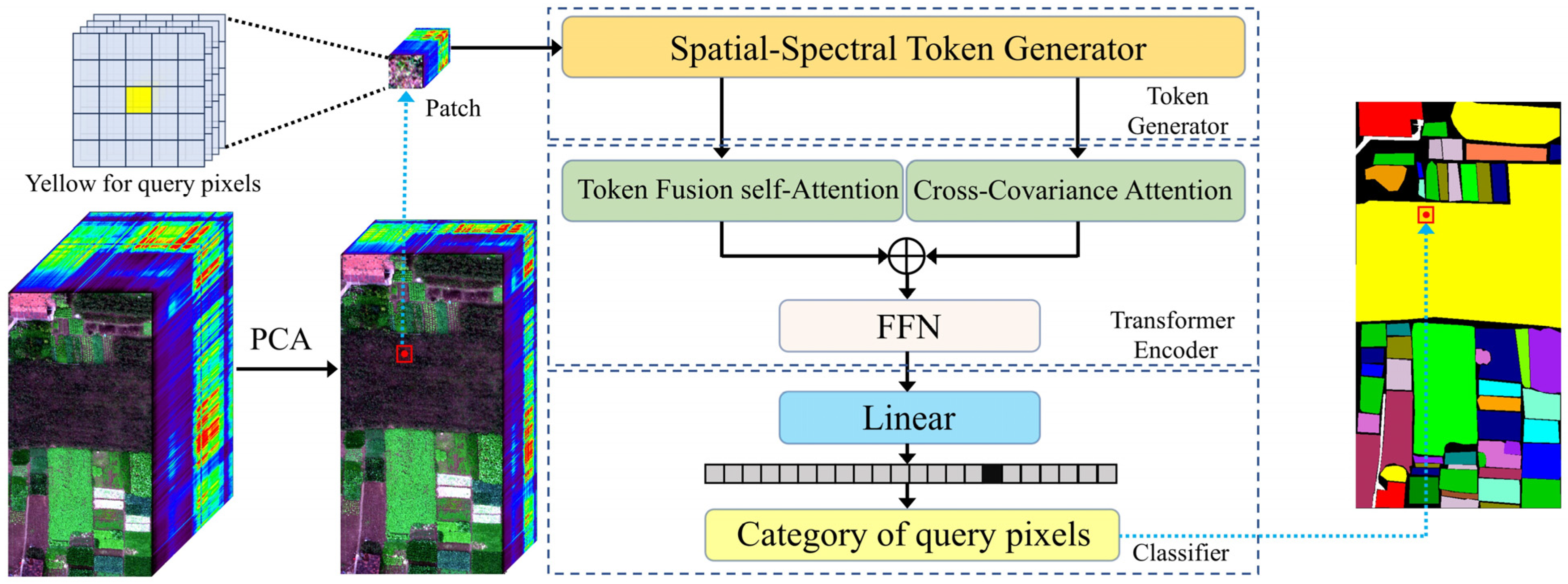
3.1. Proposed MSST Architecture
3.2. Spatial–Spectral Token Generator
3.3. Token Fusion Self-Attention
3.4. Transformer Encoder
4. Experiment and Results
4.1. Data Descriptions and Experimental Settings
4.1.1. Data Detail
4.1.2. Experimental Settings
4.2. Comparison and Analyses of Methods
4.2.1. Quantitative Results and Analysis
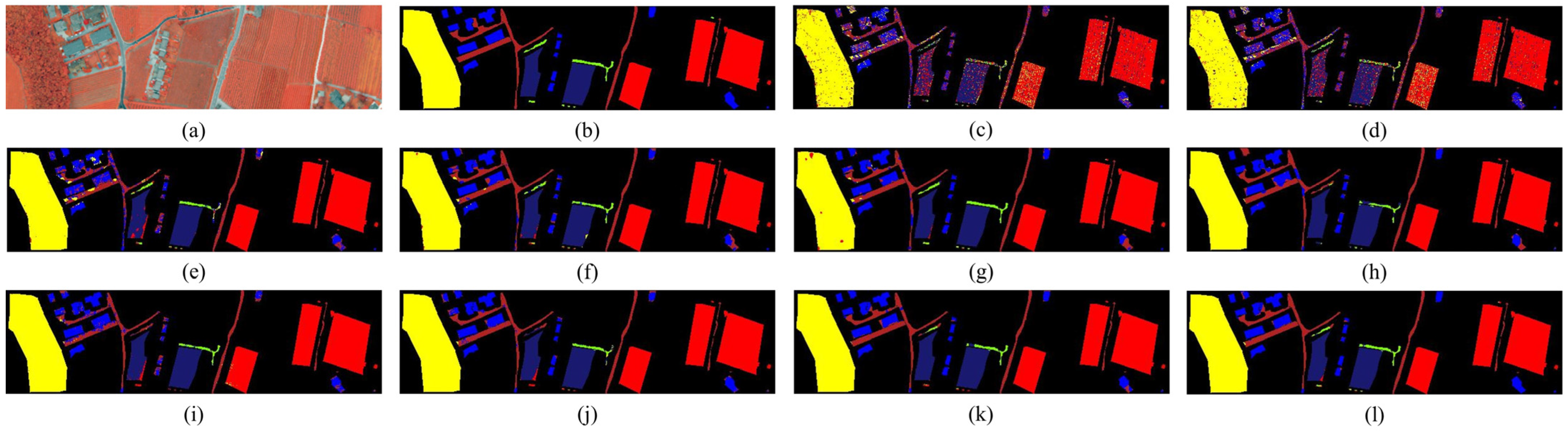
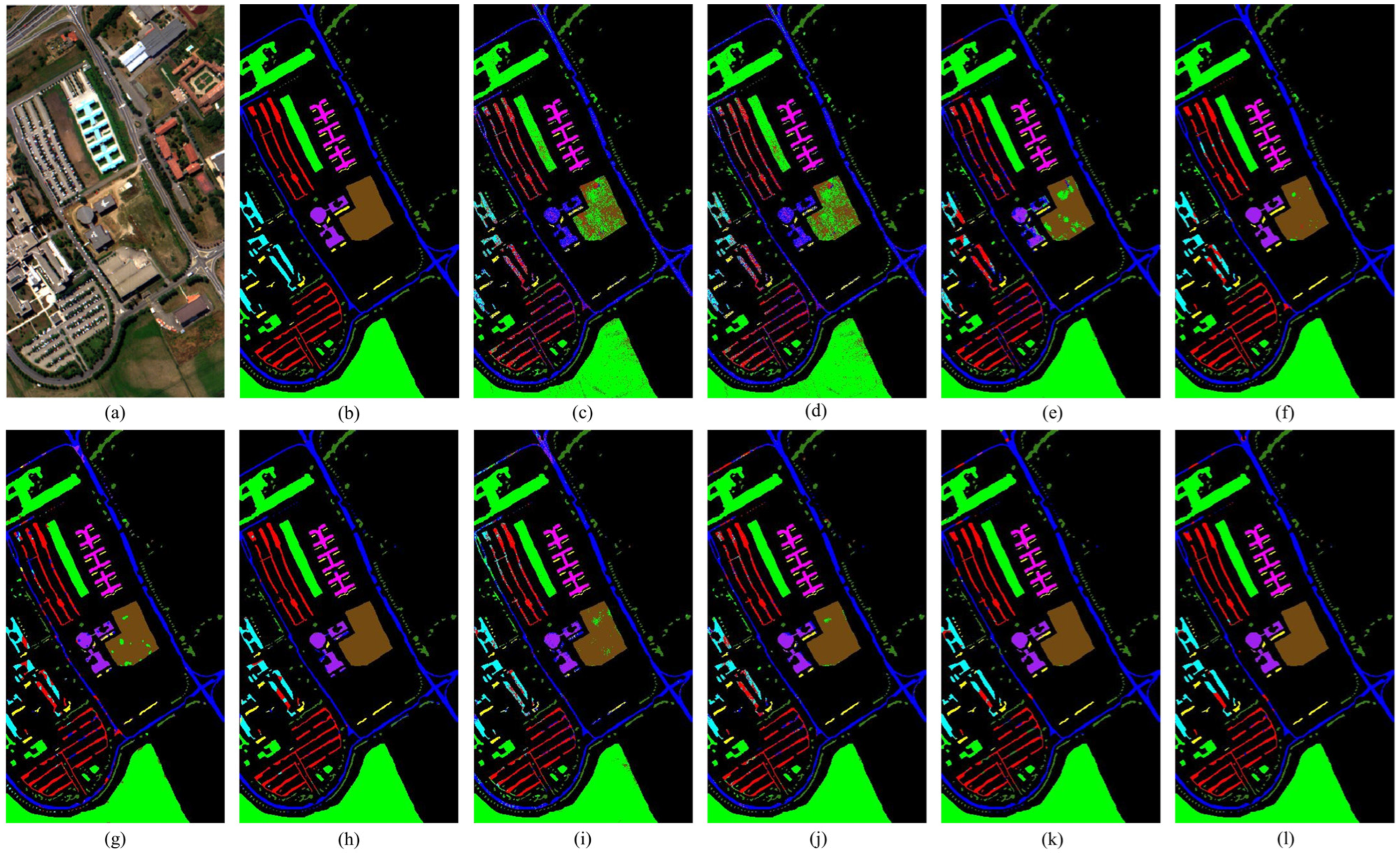
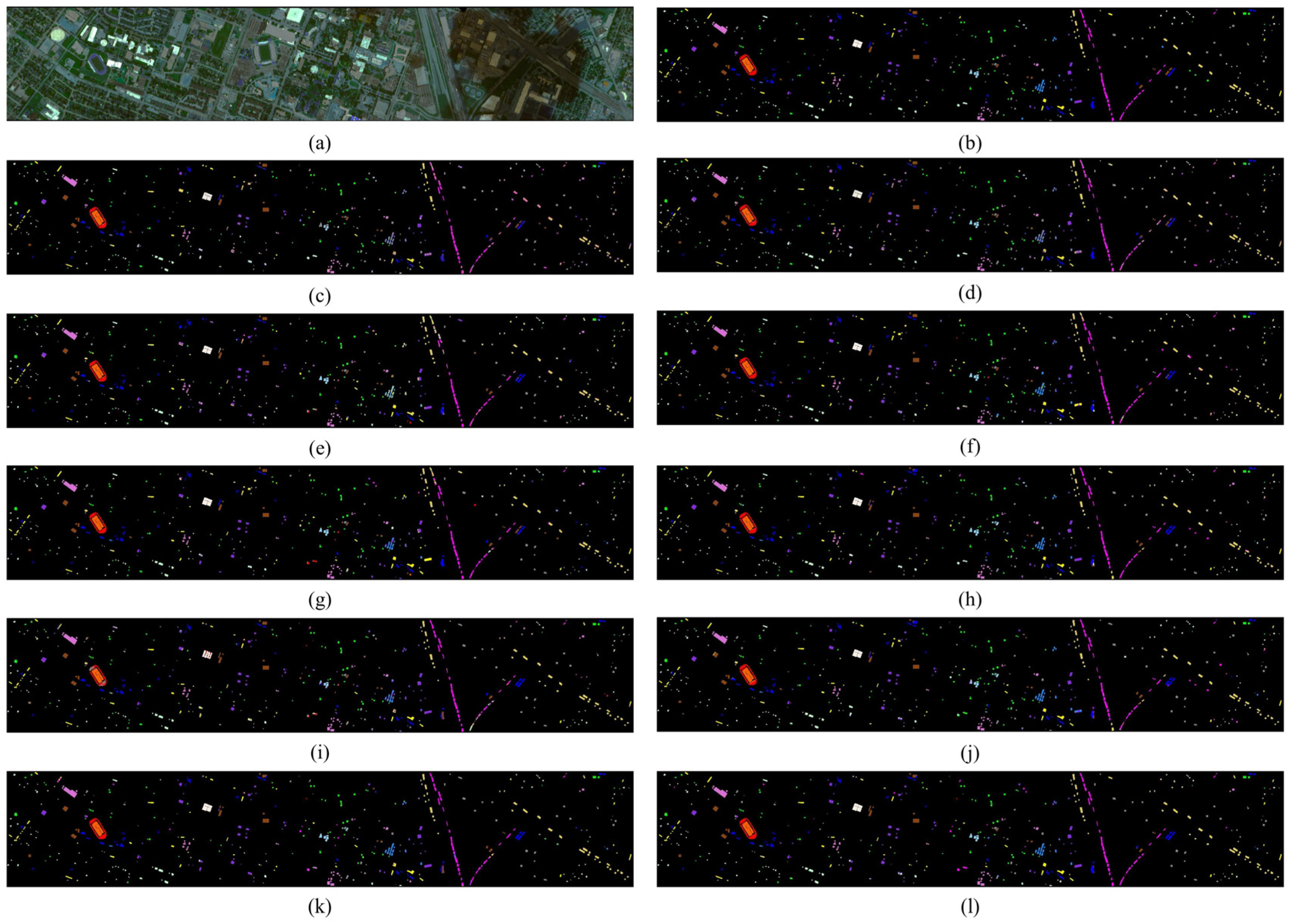
4.2.2. Qualitative Results and Analysis
4.2.3. Time Complexity Comparison
5. Discussion
5.1. Parameter Sensitivity Analysis
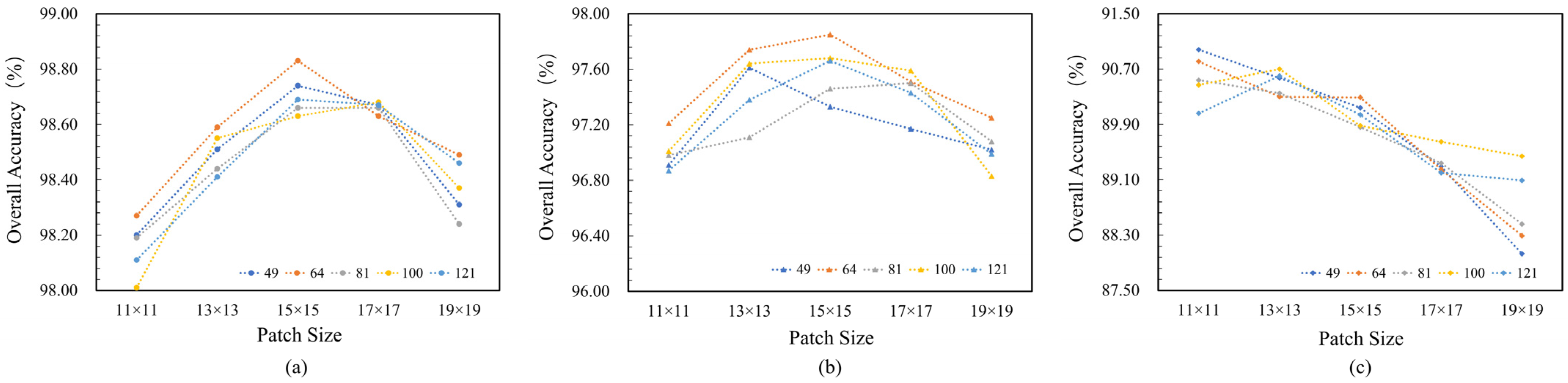
5.1.1. The Impact of Patch Size and Number of Tokens
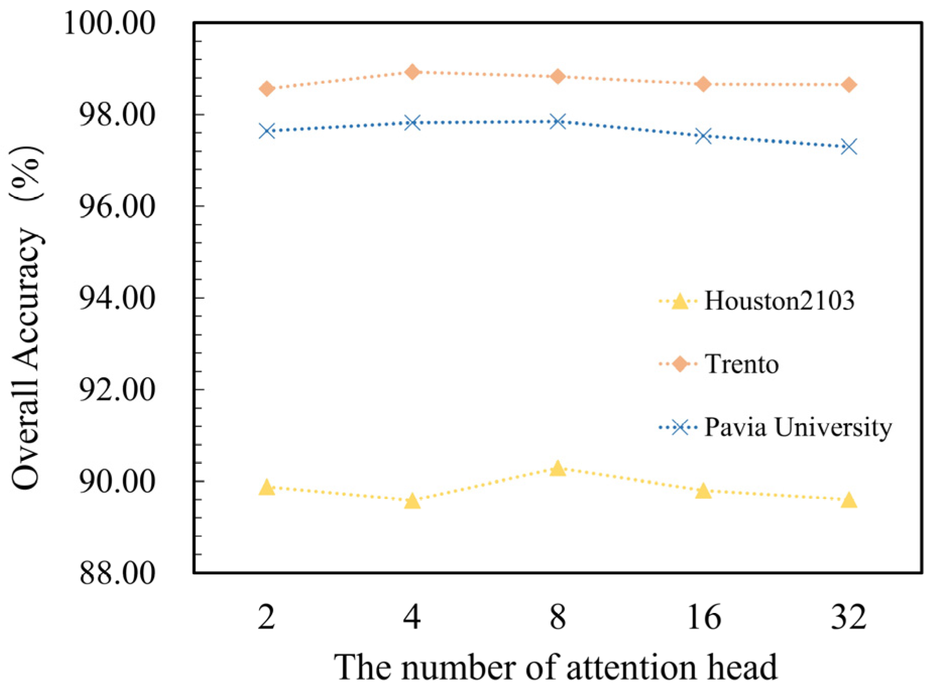
5.1.2. The Impact of the Number of Attentional Heads
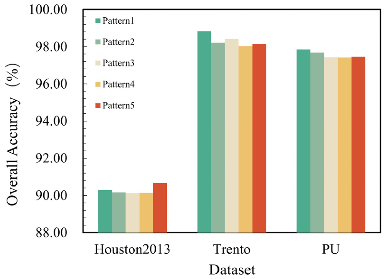
5.1.3. The Impact of Token Fusion Patterns in TFSA
5.2. Ablation Study
5.2.1. Ablation Study on the Main Modules
5.2.2. Ablation Study on the TFSA Module
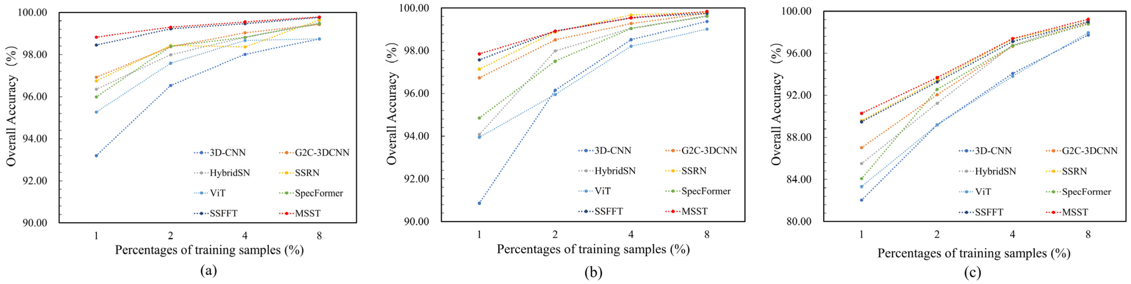
5.3. Impact of Training Data Size on Method Performance
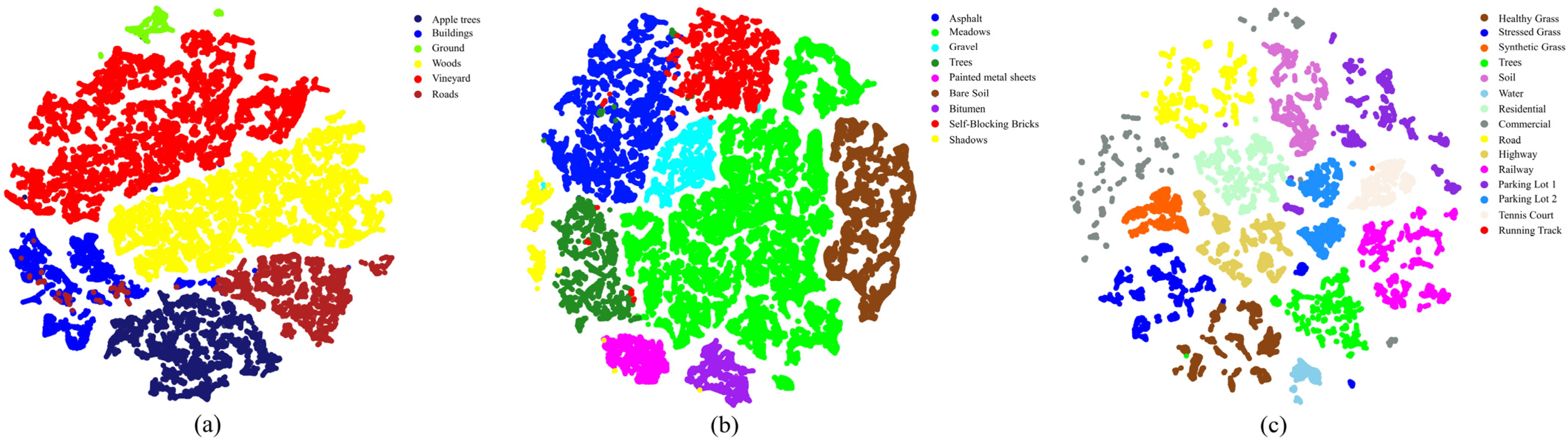
5.4. Semantic Feature Analysis
6. Conclusions
Author Contributions
Funding
Data Availability Statement
Conflicts of Interest
References
- Srivastava, P.K.; Malhi, R.K.M.; Pandey, P.C.; Anand, A.; Singh, P.; Pandey, M.K.; Gupta, A. 1—Revisiting hyperspectral remote sensing: Origin, processing, applications and way forward. In Hyperspectral Remote Sensing; Elsevier: Amsterdam, The Netherlands, 2020; pp. 3–21. [Google Scholar] [CrossRef]
- Amigo, J.M.; Babamoradi, H.; Elcoroaristizabal, S. Hyperspectral image analysis. A tutorial. Anal. Chim. Acta 2015, 896, 34–51. [Google Scholar] [CrossRef] [PubMed]
- Sima, P.; Yun, Z. Hyperspectral remote sensing in lithological mapping, mineral exploration, and environmental geology: An updated review. J. Appl. Remote Sens. 2021, 15, 031501. [Google Scholar]
- Saha, D.; Manickavasagan, A. Machine learning techniques for analysis of hyperspectral images to determine quality of food products: A review. Curr. Res. Food Sci. 2021, 4, 28–44. [Google Scholar] [CrossRef] [PubMed]
- Wieme, J.; Mollazade, K.; Malounas, I.; Zude-Sasse, M.; Zhao, M.; Gowen, A.; Argyropoulos, D.; Fountas, S.; Van Beek, J. Application of hyperspectral imaging systems and artificial intelligence for quality assessment of fruit, vegetables and mushrooms: A review. Biosyst. Eng. 2022, 222, 156–176. [Google Scholar] [CrossRef]
- Pathan, S.; Azade, S.Y.; Sawane, D.V.; Khan, S.N. Hyperspectral Image Classification: A Review. In Proceedings of the International Conference on Applications of Machine Intelligence and Data Analytics (ICAMIDA 2022), Aurangabad, India, 22–24 December 2022; Atlantis Press: Dordrecht, The Netherlands, 2023; pp. 582–591. [Google Scholar]
- Cheng, G.; Han, J.; Guo, L.; Liu, Z.; Bu, S.; Ren, J. Effective and Efficient Midlevel Visual Elements-Oriented Land-Use Classification Using VHR Remote Sensing Images. IEEE Trans. Geosci. Remote Sens. 2015, 53, 4238–4249. [Google Scholar] [CrossRef]
- Ni, D.; Ma, H. Hyperspectral Image Classification via Sparse Code Histogram. IEEE Geosci. Remote Sens. Lett. 2015, 12, 1843–1847. [Google Scholar]
- Zhang, L.; Zhang, L.; Du, B. Deep Learning for Remote Sensing Data: A Technical Tutorial on the State of the Art. IEEE Geosci. Remote Sens. Mag. 2016, 4, 22–40. [Google Scholar] [CrossRef]
- He, L.; Li, J.; Liu, C.; Li, S. Recent Advances on Spectral–Spatial Hyperspectral Image Classification: An Overview and New Guidelines. IEEE Trans. Geosci. Remote Sens. 2018, 56, 1579–1597. [Google Scholar] [CrossRef]
- Uddin, M.P.; Mamun, M.A.; Hossain, M.A. PCA-based Feature Reduction for Hyperspectral Remote Sensing Image Classification. IETE Technol. Rev. 2021, 38, 377–396. [Google Scholar] [CrossRef]
- Zhu, C.; Ding, J.; Zhang, Z.; Wang, Z. Exploring the potential of UAV hyperspectral image for estimating soil salinity: Effects of op-timal band combination algorithm and random forest. Spectrochim. Acta Part A Mol. Biomol. Spectrosc. 2022, 279, 121416. [Google Scholar] [CrossRef]
- Okwuashi, O.; Ndehedehe, C.E. Deep support vector machine for hyperspectral image classification. Pattern Recognit. 2020, 103, 107298. [Google Scholar] [CrossRef]
- Peng, J.; Sun, W.; Li, W.; Li, H.-C.; Meng, X.; Ge, C.; Du, Q. Low-Rank and Sparse Representation for Hyperspectral Image Processing: A review. IEEE Geosci. Remote Sens. Mag. 2022, 10, 10–43. [Google Scholar] [CrossRef]
- Hou, Z.; Li, W.; Li, L.; Tao, R.; Du, Q. Hyperspectral Change Detection Based on Multiple Morphological Profiles. IEEE Trans. Geosci. Remote Sens. 2022, 60, 1–12. [Google Scholar] [CrossRef]
- Tao, M.; Yunfei, L.; Weijian, H.; Chun, W.; Shuangquan, G. Hyperspectral remote sensing image semantic segmentation using extended extrema morphological profiles. In Proceedings of the Fourteenth International Conference on Digital Image Processing (ICDIP 2022), Wuhan, China, 20–23 May 2022. [Google Scholar]
- Hong, D.; Hu, J.; Yao, J.; Chanussot, J.; Zhu, X.X. Multimodal remote sensing benchmark datasets for land cover classification with a shared and specific feature learning model. ISPRS J. Photogramm. Remote Sens. 2021, 178, 68–80. [Google Scholar] [CrossRef] [PubMed]
- Huang, F.; Lu, J.; Tao, J.; Li, L.; Tan, X.; Liu, P. Research on Optimization Methods of ELM Classification Algorithm for Hyperspectral Remote Sensing Images. IEEE Access 2019, 7, 108070–108089. [Google Scholar] [CrossRef]
- Ergul, U.; Bilgin, G. MCK-ELM: Multiple composite kernel extreme learning machine for hyperspectral images. Neural Comput. Appl. 2020, 32, 6809–6819. [Google Scholar] [CrossRef]
- Ahmad, M.; Shabbir, S.; Roy, S.K.; Hong, D.; Wu, X.; Yao, J.; Khan, A.M.; Mazzara, M.; Distefano, S.; Chanussot, J. Hyperspectral Image Classification—Traditional to Deep Models: A Survey for Future Prospects. IEEE J. Sel. Top. Appl. Earth Obs. Remote Sens. 2022, 15, 968–999. [Google Scholar] [CrossRef]
- Tao, H. A label-relevance multi-direction interaction network with enhanced deformable convolution for forest smoke recognition. Expert Syst. Appl. 2024, 236, 121383. [Google Scholar] [CrossRef]
- Le, N.; Rathour, V.S.; Yamazaki, K.; Luu, K.; Savvides, M. Deep reinforcement learning in computer vision: A comprehensive survey. Artif. Intell. Rev. 2022, 55, 2733–2819. [Google Scholar] [CrossRef]
- Zhou, P.; Han, J.; Cheng, G.; Zhang, B. Learning Compact and Discriminative Stacked Autoencoder for Hyperspectral Image Classification. IEEE Trans. Geosci. Remote Sens. 2019, 57, 4823–4833. [Google Scholar] [CrossRef]
- Yao, D.; Zhi-Li, Z.; Xiao-Feng, Z.; Wei, C.; Fang, H.; Yao-Ming, C.; Cai, W.-W. Deep hybrid: Multi-graph neural network collaboration for hyperspectral image classification. Def. Technol. 2023, 23, 164–176. [Google Scholar] [CrossRef]
- Wang, J.; Guo, S.; Huang, R.; Li, L.; Zhang, X.; Jiao, L. Dual-Channel Capsule Generation Adversarial Network for Hyperspectral Image Classification. IEEE Trans. Geosci. Remote Sens. 2022, 60, 5501016. [Google Scholar] [CrossRef]
- Vaddi, R.; Manoharan, P. Hyperspectral image classification using CNN with spectral and spatial features integration. Infrared Phys. Technol. 2020, 107, 103296. [Google Scholar] [CrossRef]
- Ma, X.; Wang, H.; Geng, J. Spectral–Spatial Classification of Hyperspectral Image Based on Deep Auto-Encoder. IEEE J. Sel. Top. Appl. Earth Obs. Remote Sens. 2016, 9, 4073–4085. [Google Scholar] [CrossRef]
- Pang, L.; Men, S.; Yan, L.; Xiao, J. Rapid Vitality Estimation and Prediction of Corn Seeds Based on Spectra and Images Using Deep Learning and Hyperspectral Imaging Techniques. IEEE Access 2020, 8, 123026–123036. [Google Scholar] [CrossRef]
- He, N.; Paoletti, M.E.; Haut, J.N.M.; Fang, L.; Li, S.; Plaza, A.; Plaza, J. Feature Extraction With Multiscale Covariance Maps for Hyperspectral Image Classification. IEEE Trans. Geosci. Remote Sens. 2019, 57, 755–769. [Google Scholar] [CrossRef]
- Xu, H.; Yao, W.; Cheng, L.; Li, B. Multiple Spectral Resolution 3D Convolutional Neural Network for Hyperspectral Image Classification. Remote Sens. 2021, 13, 1248. [Google Scholar] [CrossRef]
- Roy, S.K.; Krishna, G.; Dubey, S.R.; Chaudhuri, B.B. HybridSN: Exploring 3-D–2-D CNN Feature Hierarchy for Hyperspectral Image Classification. IEEE Geosci. Remote Sens. Lett. 2020, 17, 277–281. [Google Scholar] [CrossRef]
- Zhong, Z.; Li, J.; Luo, Z.; Chapman, M. Spectral–Spatial Residual Network for Hyperspectral Image Classification: A 3-D Deep Learning Framework. IEEE Trans. Geosci. Remote Sens. 2018, 56, 847–858. [Google Scholar] [CrossRef]
- Liu, D.; Wang, Y.; Liu, P.; Li, Q.; Yang, H.; Chen, D.; Liu, Z.; Han, G. A Multiscale Cross Interaction Attention Network for Hyperspectral Image Classification. Remote Sens. 2023, 15, 428. [Google Scholar] [CrossRef]
- Paheding, S.; Reyes, A.A.; Kasaragod, A.; Oommen, T. GAF-NAU: Gramian angular field encoded neighborhood attention U-Net for pixel-wise hyperspectral image classification. In Proceedings of the IEEE/CVF Conference on Computer Vision and Pattern Recognition, New Orleans, LA, USA, 18–24 June 2022; pp. 409–417. [Google Scholar]
- Zhu, J.; Fang, L.; Ghamisi, P. Deformable Convolutional Neural Networks for Hyperspectral Image Classification. IEEE Geosci. Remote Sens. Lett. 2018, 15, 1254–1258. [Google Scholar] [CrossRef]
- Qing, Y.; Liu, W.; Feng, L.; Gao, W. Improved Transformer Net for Hyperspectral Image Classification”, 2021 Remote Sensing.
- Ouyang, E.; Li, B.; Hu, W.; Zhang, G.; Zhao, L.; Wu, J. When Multigranularity Meets Spatial–Spectral Attention: A Hybrid Transformer for Hyperspectral Image Classification. IEEE Trans. Geosci. Remote Sens. 2023, 61, 4401118. [Google Scholar] [CrossRef]
- Devlin, J.; Chang, M.W.; Lee, K.; Toutanova, K. Bert: Pre-training of deep bidirectional transformers for language understanding. arXiv 2018, arXiv:1810.04805. [Google Scholar]
- Meyer, J.G.; Urbanowicz, R.J.; Martin, P.C.N.; O’connor, K.; Li, R.; Peng, P.-C.; Bright, T.J.; Tatonetti, N.; Won, K.J.; Gonzalez-Hernandez, G.; et al. ChatGPT and large language models in academia: Opportunities and challenges. BioData Min. 2023, 16, 20. [Google Scholar] [CrossRef]
- Dosovitskiy, A.; Beyer, L.; Kolesnikov, A.; Weissenborn, D.; Zhai, X.; Unterthiner, T.; Dehghani, M.; Minderer, M.; Heigold, G.; Gelly, S.; et al. An image is worth 16x16 words: Transformers for image recognition at scale. arXiv 2020, arXiv:2010.11929. [Google Scholar]
- Han, K.; Wang, Y.; Chen, H.; Chen, X.; Guo, J.; Liu, Z.; Tang, Y.; Xiao, A.; Xu, C.; Xu, Y.; et al. A survey on vision transformer. IEEE Trans. Pattern Anal. Mach. Intell. 2022, 45, 87–110. [Google Scholar] [CrossRef] [PubMed]
- He, X.; Chen, Y.; Lin, Z. Spatial-Spectral Transformer for Hyperspectral Image Classification. Remote Sens. 2021, 13, 498. [Google Scholar] [CrossRef]
- Roy, S.K.; Deria, A.; Shah, C.; Haut, J.M.; Du, Q.; Plaza, A. Spectral–Spatial Morphological Attention Transformer for Hyperspectral Image Classification. IEEE Trans. Geosci. Remote Sens. 2023, 61, 5503615. [Google Scholar] [CrossRef]
- Roy, S.K.; Deria, A.; Hong, D.; Rasti, B.; Plaza, A.; Chanussot, J. Multimodal Fusion Transformer for Remote Sensing Image Classification. IEEE Trans. Geosci. Remote Sens. 2023, 61, 5515620. [Google Scholar] [CrossRef]
- Mei, S.; Song, C.; Ma, M.; Xu, F. Hyperspectral image classification using group-aware hierarchical transformer. IEEE Trans. Geosci. Remote Sens. 2022, 60, 5539014. [Google Scholar] [CrossRef]
- Chen CF, R.; Fan, Q.; Panda, R. Crossvit: Cross-attention multi-scale vision transformer for image classification. In Proceedings of the IEEE/CVF International Conference on Computer Vision, Virtual, 11–17 October 2021; pp. 357–366. [Google Scholar]
- Liu, Z.; Lin, Y.; Cao, Y.; Hu, H.; Wei, Y.; Zhang, Z.; Lin, S.; Guo, B. Swin transformer: Hierarchical vision transformer using shifted windows. In Proceedings of the IEEE/CVF International Conference on Computer Vision, Montreal, BC, Canada, 11–17 October 2021; pp. 10012–10022. [Google Scholar]
- Ali, A.; Touvron, H.; Caron, M.; Bojanowski, P.; Douze, M.; Joulin, A.; Laptev, I.; Neverova, N.; Synnaeve, G.; Verbeek, J.; et al. Xcit: Cross-covariance image transformers. Adv. Neural Inf. Process. Syst. 2021, 34, 20014–20027. [Google Scholar]
- Yang, X.; Cao, W.; Lu, Y.; Zhou, Y. Hyperspectral Image Transformer Classification Networks. IEEE Trans. Geosci. Remote Sens. 2022, 60, 5528715. [Google Scholar] [CrossRef]
- Yang, L.; Yang, Y.; Yang, J.; Zhao, N.; Wu, L.; Wang, L.; Wang, T. FusionNet: A Convolution–Transformer Fusion Network for Hyperspectral Image Classification. Remote Sens. 2022, 14, 4066. [Google Scholar] [CrossRef]
- Sun, L.; Zhao, G.; Zheng, Y.; Wu, Z. Spectral–spatial feature tokenization transformer for hyperspectral image classification. IEEE Trans. Geosci. Remote Sens. 2022, 60, 5522214. [Google Scholar] [CrossRef]
- Huang, X.; Dong, M.; Li, J.; Guo, X. A 3-D-Swin Transformer-Based Hierarchical Contrastive Learning Method for Hyperspectral Image Classification. IEEE Trans. Geosci. Remote Sens. 2022, 60, 5411415. [Google Scholar] [CrossRef]
- Wang, W.; Xie, E.; Li, X.; Fan, D.-P.; Song, K.; Liang, D.; Lu, T.; Luo, P.; Shao, L. Pyramid vision transformer: A versatile backbone for dense prediction without convolutions. In Proceedings of the IEEE/CVF International Conference on Computer Vision (ICCV), Montreal, QC, Canada, 10–17 October 2021; pp. 568–578. [Google Scholar]
- Ren, S.; Zhou, D.; He, S.; Feng, J.; Wang, X. Shunted self-attention via multi-scale token aggregation. In Proceedings of the IEEE/CVF Conference on Computer Vision and Pattern Recognition, New Orleans, LA, USA, 18–24 June 2022; pp. 10853–10862. [Google Scholar]
- Yin, J.; Qi, C.; Huang, W.; Chen, Q.; Qu, J. Multibranch 3D-Dense Attention Network for Hyperspectral Image Classification. IEEE Access 2022, 10, 71886–71898. [Google Scholar] [CrossRef]
- Roy, S.K.; Kar, P.; Hong, D.; Wu, X.; Plaza, A.; Chanussot, J. Revisiting deep hyperspectral feature extraction networks via gradient centralized convolution. IEEE Trans. Geosci. Remote Sens. 2021, 60, 5516619. [Google Scholar] [CrossRef]
- Hong, D.; Han, Z.; Yao, J.; Gao, L.; Zhang, B.; Plaza, A.; Chanussot, J. SpectralFormer: Rethinking hyperspectral image classification with transformers. IEEE Trans. Geosci. Remote Sens. 2021, 60, 5518615. [Google Scholar] [CrossRef]


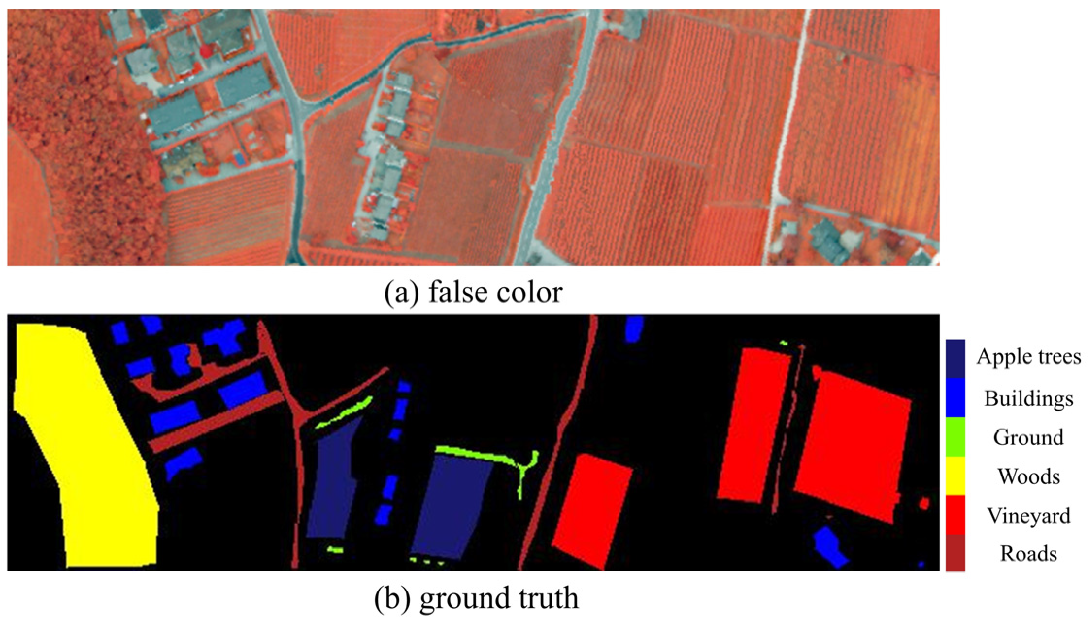
| Class No. | Color | Class Name | Test | Train | |
|---|---|---|---|---|---|
| 1 | MidnightBlue | Apple trees | 3994 | 40 | |
| 2 | Blue | Buildings | 2874 | 29 | |
| 3 | LawnGreen | Ground | 474 | 5 | |
| 4 | Yellow | Woods | 9032 | 91 | |
| 5 | Red | Vineyard | 10,396 | 105 | |
| 6 | FireBrick | Roads | 3142 | 32 | |
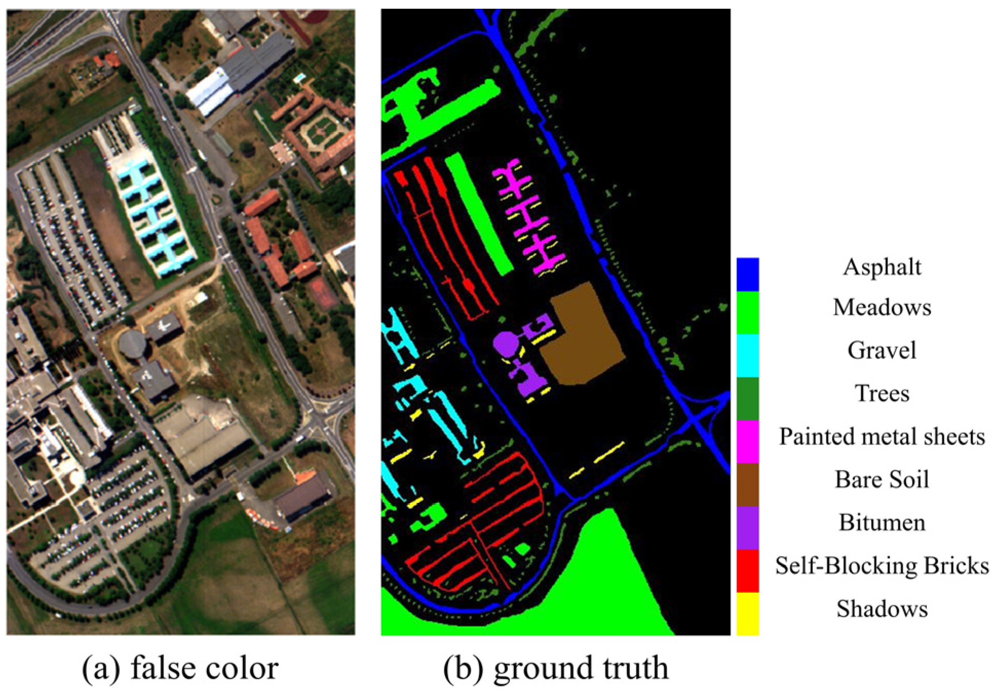
| Class No. | Color | Class Name | Test | Train | |
|---|---|---|---|---|---|
| 1 | Blue | Asphalt | 1249 | 13 | |
| 2 | Green | Meadows | 201 | 3 | |
| 3 | Cyan | Gravel | 607 | 7 | |
| 4 | ForestGreen | Trees | 148 | 2 | |
| 5 | Magenta | Painted metal sheets | 1750 | 18 | |
| 6 | SaddleBrown | Bare Soil | 357 | 4 | |
| 7 | Purple | Bitumen | 4984 | 51 | |
| 8 | Red | Self-Blocking Bricks | 6310 | 64 | |
| 9 | Yellow | Shadows | 394 | 4 | |
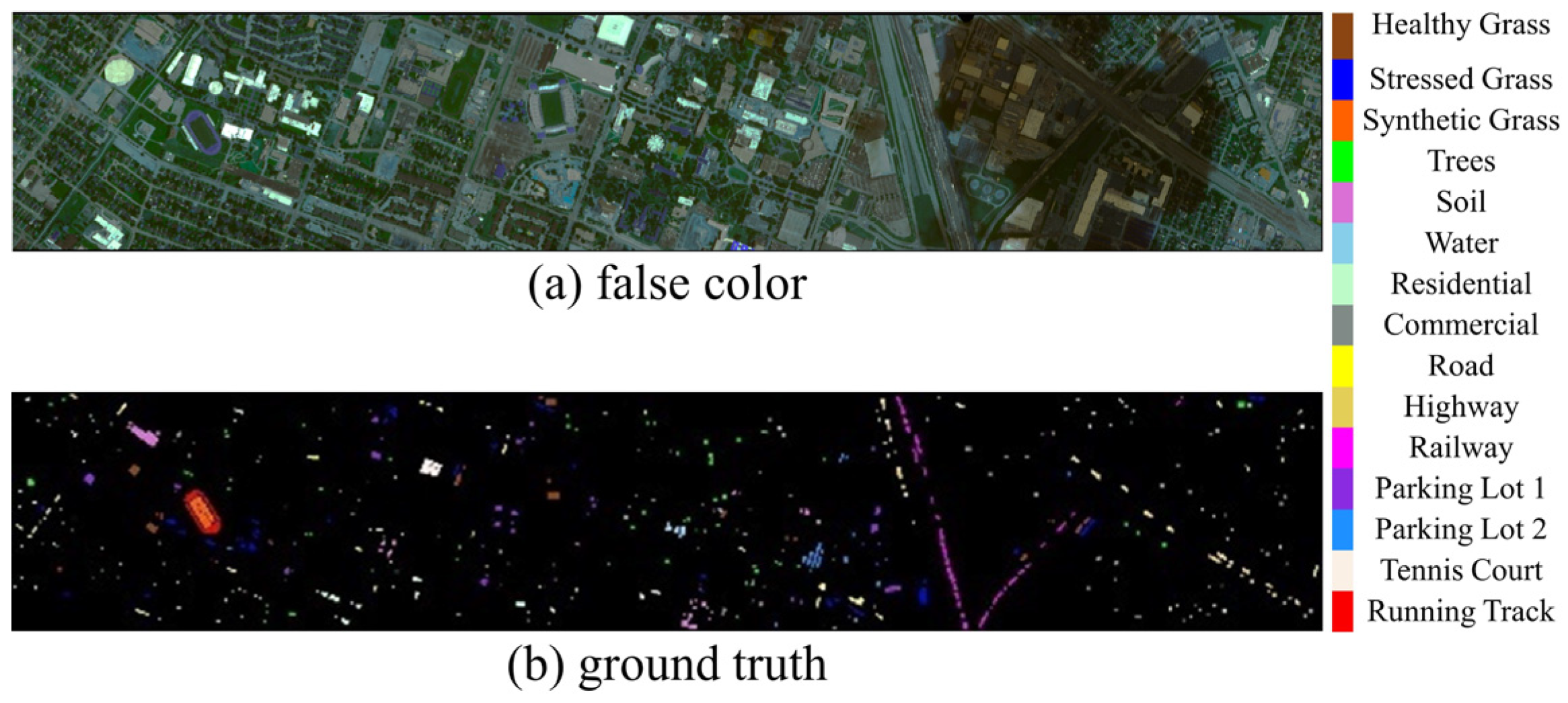
| Class No. | Color | Class Name | Test | Train | |
|---|---|---|---|---|---|
| 1 | SaddleBrown | Healthy Grass | 13,901 | 140 | |
| 2 | Blue | Stressed Grass | 3477 | 35 | |
| 3 | Orange | Synthetic Grass | 21,603 | 218 | |
| 4 | Green | Trees | 161,653 | 1632 | |
| 5 | Orchid | Soil | 6156 | 62 | |
| 6 | SkyBlue | Water | 44,111 | 446 | |
| 7 | MintGreen | Residential | 23,862 | 241 | |
| 8 | CoolGray | Commercial | 4013 | 41 | |
| 9 | Yellow | Road | 10,711 | 108 | |
| 10 | BananaYellow | Highway | 12,270 | 124 | |
| 11 | Magenta | Railway | 10,905 | 110 | |
| 12 | BlueViolet | Parking Lot 1 | 8864 | 90 | |
| 13 | DodgerBlue | Parking Lot 2 | 22,282 | 225 | |
| 14 | Linen | Tennis Court | 7282 | 74 | |
| 15 | Red | Running Track | 4000 | 40 | |
| Class | SVM | RF | 3D-CNN | G2C-3DCNN | HybridSN | SSRN | ViT | SpecFormer | SSFFT | Ours |
|---|---|---|---|---|---|---|---|---|---|---|
| 1 | 89.00 | 92.92 | 96.92 | 96.73 | 94.01 | 98.08 | 93.12 | 96.98 | 97.36 | 96.38 |
| 2 | 94.41 | 97.39 | 99.76 | 99.81 | 99.49 | 99.63 | 99.80 | 99.98 | 99.88 | 99.90 |
| 3 | 49.47 | 23.00 | 56.59 | 82.44 | 75.31 | 84.46 | 60.73 | 71.90 | 90.18 | 90.42 |
| 4 | 83.02 | 79.95 | 84.37 | 89.02 | 87.90 | 88.33 | 92.71 | 84.31 | 92.05 | 93.68 |
| 5 | 98.80 | 99.77 | 99.62 | 99.85 | 100.00 | 98.87 | 99.55 | 99.77 | 99.10 | 99.22 |
| 6 | 62.88 | 27.70 | 85.46 | 98.57 | 93.63 | 100.00 | 94.92 | 97.33 | 99.84 | 100.00 |
| 7 | 27.79 | 33.64 | 68.03 | 97.27 | 90.51 | 94.76 | 79.57 | 90.05 | 100.00 | 100.00 |
| 8 | 68.20 | 80.43 | 85.87 | 91.08 | 82.28 | 97.06 | 88.34 | 88.29 | 92.37 | 95.35 |
| 9 | 73.32 | 71.78 | 37.99 | 99.68 | 94.34 | 84.20 | 91.14 | 75.88 | 90.50 | 91.21 |
| OA (%) | 82.19 ± 0.47 | 80.04 ± 0.65 | 90.86 ± 0.41 | 96.73 ± 0.24 | 94.08 ± 0.40 | 97.14 ± 0.23 | 93.95 ± 0.54 | 94.85 ± 0.10 | 97.57 ± 0.08 | 97.85 ± 0.24 |
| AA (%) | 71.88 ± 0.66 | 67.40 ± 0.74 | 79.40 ± 0.26 | 94.94 ± 0.21 | 90.83 ± 0.32 | 93.93 ± 0.18 | 88.88 ± 0.61 | 89.39 ± 0.25 | 95.70 ± 0.20 | 96.24 ± 0.05 |
| K × 100 | 75.94 ± 0.42 | 72.50 ± 0.50 | 87.70 ± 0.14 | 95.65 ± 0.15 | 92.11 ± 0.18 | 96.21 ± 0.06 | 91.93 ± 0.51 | 93.12 ± 0.28 | 96.78 ± 0.33 | 97.16 ± 0.37 |
| Class | SVM | RF | 3D-CNN | G2C-3DCNN | HybridSN | SSRN | ViT | SpecFormer | SSFFT | Ours |
|---|---|---|---|---|---|---|---|---|---|---|
| 1 | 78.14 | 68.70 | 97.65 | 98.87 | 99.70 | 99.17 | 96.52 | 98.97 | 99.67 | 99.65 |
| 2 | 59.19 | 64.65 | 66.74 | 82.67 | 85.32 | 88.45 | 84.06 | 90.22 | 94.33 | 95.72 |
| 3 | 31.01 | 36.71 | 49.16 | 83.33 | 81.86 | 46.62 | 36.50 | 22.36 | 57.38 | 81.22 |
| 4 | 95.26 | 94.39 | 99.09 | 99.92 | 99.03 | 100.00 | 99.75 | 100.00 | 99.98 | 99.98 |
| 5 | 85.58 | 90.22 | 99.89 | 100.00 | 99.72 | 100.00 | 99.99 | 99.95 | 99.97 | 100.00 |
| 6 | 66.65 | 77.94 | 79.28 | 90.07 | 85.55 | 88.77 | 84.28 | 83.96 | 97.45 | 96.12 |
| OA (%) | 82.12 ± 1.02 | 84.01 ± 0.74 | 93.20 ± 0.37 | 96.92 ± 0.17 | 96.35 ± 0.38 | 96.75 ± 0.10 | 95.27 ± 0.41 | 95.99 ± 0.24 | 98.45 ± 0.08 | 98.83 ± 0.38 |
| AA (%) | 69.30 ± 0.84 | 72.10 ± 0.58 | 81.97 ± 0.32 | 92.58 ± 0.34 | 91.86 ± 0.15 | 87.17 ± 0.07 | 83.52 ± 0.55 | 82.58 ± 0.10 | 91.46 ± 0.15 | 95.45 ± 0.20 |
| K × 100 | 76.00 ± 0.80 | 78.43 ± 0.66 | 90.86 ± 0.24 | 95.88 ± 0.20 | 95.13 ± 0.26 | 95.66 ± 0.07 | 93.66 ± 0.34 | 94.64 ± 0.14 | 97.93 ± 0.18 | 98.44 ± 0.18 |
| Class | SVM | RF | 3D-CNN | G2C-3DCNN | HybridSN | SSRN | ViT | SpecFormer | SSFFT | Ours |
|---|---|---|---|---|---|---|---|---|---|---|
| 1 | 96.40 | 96.32 | 89.01 | 86.62 | 98.01 | 86.03 | 84.49 | 87.87 | 86.47 | 89.12 |
| 2 | 87.57 | 96.04 | 82.37 | 91.67 | 95.63 | 90.28 | 95.63 | 93.16 | 95.90 | 92.85 |
| 3 | 99.62 | 99.75 | 97.78 | 97.97 | 94.54 | 97.20 | 95.55 | 94.16 | 95.93 | 95.43 |
| 4 | 90.57 | 90.25 | 88.49 | 89.05 | 89.69 | 93.76 | 83.21 | 89.49 | 81.14 | 91.13 |
| 5 | 97.59 | 99.46 | 99.77 | 100.00 | 99.30 | 100.00 | 99.46 | 99.77 | 100.00 | 100.00 |
| 6 | 45.24 | 61.01 | 83.63 | 83.33 | 84.82 | 86.31 | 83.33 | 61.76 | 86.31 | 86.31 |
| 7 | 81.66 | 81.66 | 63.72 | 67.28 | 74.81 | 79.95 | 75.63 | 67.45 | 74.06 | 72.35 |
| 8 | 76.57 | 68.43 | 67.31 | 72.46 | 65.75 | 70.00 | 80.97 | 77.54 | 78.06 | 76.87 |
| 9 | 68.88 | 79.27 | 64.72 | 77.26 | 77.52 | 88.43 | 79.53 | 76.16 | 80.25 | 79.40 |
| 10 | 78.23 | 79.50 | 94.90 | 99.08 | 96.95 | 100.00 | 99.72 | 98.98 | 100.00 | 99.57 |
| 11 | 79.94 | 87.87 | 76.68 | 87.29 | 74.39 | 88.00 | 64.45 | 83.39 | 95.48 | 98.06 |
| 12 | 69.89 | 68.90 | 90.04 | 94.49 | 75.76 | 91.95 | 94.70 | 93.71 | 98.16 | 98.09 |
| 13 | 23.80 | 12.78 | 50.32 | 65.50 | 68.05 | 81.63 | 31.79 | 39.54 | 73.00 | 80.35 |
| 14 | 86.61 | 96.46 | 90.16 | 99.61 | 100.00 | 99.02 | 68.31 | 70.97 | 100.00 | 100.00 |
| 15 | 96.08 | 97.09 | 99.69 | 99.37 | 100.00 | 99.37 | 84.05 | 84.69 | 100.00 | 100.00 |
| OA (%) | 81.02 ± 0.34 | 83.14 ± 0.27 | 82.03 ± 0.21 | 87.02 ± 0.48 | 85.51 ± 0.16 | 89.59 ± 0.41 | 83.32 ± 0.58 | 84.07 ± 0.15 | 89.48 ± 0.10 | 90.29 ± 0.12 |
| AA (%) | 78.58 ± 0.62 | 80.99 ± 0.29 | 82.57 ± 0.18 | 87.40 ± 0.30 | 86.35 ± 0.29 | 90.10 ± 0.64 | 81.39 ± 0.60 | 81.24 ± 0.08 | 89.65 ± 0.07 | 90.63 ± 0.08 |
| K × 100 | 79.45 ± 0.33 | 81.74 ± 0.53 | 80.56 ± 0.15 | 85.96 ± 0.23 | 84.34 ± 0.08 | 88.75 ± 0.28 | 81.94 ± 0.52 | 82.74 ± 0.22 | 88.62 ± 0.28 | 89.50 ± 0.27 |
| Methods | Train(S) | Test(S) | ||||
|---|---|---|---|---|---|---|
| Trento | PU | Houston 2013 | Trento | PU | Houston 2013 | |
| 3DCNN | 127.99 | 174.96 | 103.97 | 2.65 | 3.12 | 1.53 |
| G2C-3DCNN | 122.41 | 192.26 | 101.98 | 2.51 | 4.37 | 1.34 |
| HybridSN | 124.03 | 163.80 | 95.05 | 2.22 | 3.84 | 1.58 |
| SSRN | 165.22 | 200.15 | 122.02 | 3.37 | 4.54 | 2.23 |
| ViT | 188.06 | 236.09 | 145.92 | 4.56 | 6.12 | 3.40 |
| SpecFormer | 187.24 | 227.10 | 142.248 | 4.01 | 5.71 | 2.90 |
| SSFTT | 145.59 | 183.85 | 116.71 | 3.22 | 3.79 | 2.17 |
| MSST | 185.72 | 222.32 | 123.47 | 4.12 | 5.44 | 2.94 |
| Pattern1 | Pattern2 | Pattern3 | Pattern4 | Pattern5 |
|---|---|---|---|---|
| Case | Components | Dataset | ||||
|---|---|---|---|---|---|---|
| SSTG | TFSA | CCA | Houston 2013 | Trento | PU | |
| 1 | × | × | × | 83.49 | 95.45 | 93.15 |
| 2 | √ | × | × | 88.85 | 97.05 | 96.22 |
| 3 | × | √ | × | 89.65 | 97.49 | 95.57 |
| 4 | √ | √ | × | 90.01 | 98.68 | 97.80 |
| 5 | × | √ | √ | 89.46 | 97.62 | 96.85 |
| 6 | √ | √ | √ | 90.29 | 98.83 | 97.85 |
| Case | Components | Dataset | |||
|---|---|---|---|---|---|
| Main Branch | Query Pixel Branch | Houston 2013 | Trento | PU | |
| 1 | √ | × | 89.67 | 98.81 | 97.44 |
| 2 | × | √ | 84.18 | 93.73 | 94.62 |
| 3 | √ | √ | 90.29 | 98.83 | 97.85 |
Disclaimer/Publisher’s Note: The statements, opinions and data contained in all publications are solely those of the individual author(s) and contributor(s) and not of MDPI and/or the editor(s). MDPI and/or the editor(s) disclaim responsibility for any injury to people or property resulting from any ideas, methods, instructions or products referred to in the content. |
© 2024 by the authors. Licensee MDPI, Basel, Switzerland. This article is an open access article distributed under the terms and conditions of the Creative Commons Attribution (CC BY) license (https://creativecommons.org/licenses/by/4.0/).
Share and Cite
Ma, Y.; Lan, Y.; Xie, Y.; Yu, L.; Chen, C.; Wu, Y.; Dai, X. A Spatial–Spectral Transformer for Hyperspectral Image Classification Based on Global Dependencies of Multi-Scale Features. Remote Sens. 2024, 16, 404. https://doi.org/10.3390/rs16020404
Ma Y, Lan Y, Xie Y, Yu L, Chen C, Wu Y, Dai X. A Spatial–Spectral Transformer for Hyperspectral Image Classification Based on Global Dependencies of Multi-Scale Features. Remote Sensing. 2024; 16(2):404. https://doi.org/10.3390/rs16020404
Chicago/Turabian StyleMa, Yunxuan, Yan Lan, Yakun Xie, Lanxin Yu, Chen Chen, Yusong Wu, and Xiaoai Dai. 2024. "A Spatial–Spectral Transformer for Hyperspectral Image Classification Based on Global Dependencies of Multi-Scale Features" Remote Sensing 16, no. 2: 404. https://doi.org/10.3390/rs16020404
APA StyleMa, Y., Lan, Y., Xie, Y., Yu, L., Chen, C., Wu, Y., & Dai, X. (2024). A Spatial–Spectral Transformer for Hyperspectral Image Classification Based on Global Dependencies of Multi-Scale Features. Remote Sensing, 16(2), 404. https://doi.org/10.3390/rs16020404