Article

Analysis of Atmospheric Elements in Near Space Based on Meteorological-Rocket Soundings over the East China Sea

The College of Meteorology and Oceanography, National University of Defense Technology, Changsha 410005, China
*
Author to whom correspondence should be addressed.
Remote Sens. 2024, 16(2), 402; https://doi.org/10.3390/rs16020402
Submission received: 18 December 2023 / Revised: 15 January 2024 / Accepted: 16 January 2024 / Published: 20 January 2024

Abstract

:
As an important means of in situ detection in near space, meteorological rockets can provide a high-precision distribution analysis of atmospheric elements. However, there are currently few studies on the principles of meteorological-rocket detection and the application of rocket-sounding data. The purpose of this paper is to fill this gap by providing a detailed introduction to the detection principle of a meteorological rocket launched in the East China Sea in November 2022. Moreover, empirical models, satellite data, and reanalysis data were selected for comparison and verification with the rocket-sounding data. Furthermore, the accuracy of these widely used datasets was studied based on the rocket-sounding data in the near space over the East China Sea. Additionally, gravity-wave power–frequency spectra were extracted using the maximum entropy method from both the rocket-sounding data and the remote-sensing data. Furthermore, the relationship between gravity waves and Kelvin–Helmholtz instability (KHI) was investigated by analyzing the gravity-wave energy and the Richardson number. The research findings indicate that among the remote-sensing data describing the atmospheric environment over the launch site, the COSMIC occultation data is more accurate compared with the SABER data. The wind-field distribution derived from rocket detection is consistent with the Modern-Era Retrospective analysis for Research and Applications (MERRA) reanalysis data, while also providing a more detailed description of the wind field. The main wavelengths of gravity waves extracted from rocket-sounding data are consistently smaller than those obtained from satellite remote-sensing data, indicating that rocket sounding is capable of capturing more intricate structures of gravity waves. The good correspondence between the peaks of gravity-wave energy and the regions where KHI occurs indicates that there is a strong interaction between gravity waves and KHI in the middle atmosphere.

Graphical Abstract

1. Introduction

Near space generally refers to the airspace between 20 km and 100 km in altitude, which includes the stratosphere, mesosphere, and low thermosphere. With the emergence of new generation near-space vehicles such as unmanned aerial vehicles (UAVs) and near-space airships, the support for their flight missions requires near-space detection [1]. Currently, common methods for near-space detection include radiosondes [2,3], remote sensing [4,5,6,7,8], and meteorological rockets [9,10]. As a widely used detection method, radiosondes can detect a variety of atmospheric elements above the release point. However, the maximum ascent height is limited to around 30–40 km. Satellite detection methods can acquire global observations, but there are strict local time requirements for the same observation point. Radar detection has sparse and fixed stations. Meteorological-rocket sounding is the only in situ means to directly and accurately measure the atmospheric environment in near space. Its detection data is widely used in the study of the structure and element distribution of the middle and upper atmospheres [11,12,13,14]. Currently, the two most widely used technologies for meteorological rockets are the measurement of atmospheric temperature using a thermistor and the measurement of atmospheric density and wind field using the falling-sphere method [15].
The high data precision and wide detection range of meteorological rockets make them widely used in research on the accuracy of satellite data and atmospheric empirical models [1]. Based on the data from meteorological rockets launched in the northwest region of China in 2004, the accuracy of the wind-field data from the atmospheric empirical models and the temperature data observed by SABER at that location were analyzed [16]. Jiang G. et al. [17] analyzed the results of the meteorological-rocket soundings conducted as part of the Meridian Space Weather Monitoring Project and investigated the atmospheric stability over the launch site. Ge. et al. [15] carried out research on a falling-sphere experiment in northwest China and used the position data and the NRLMSISE-00 model data as input to derive the wind profiles. It was concluded that the inaccuracy of model density has little effect on the calculated wind speed and direction. Zhou et al. [11] analyzed the acquisition rate and data accuracy of the experimental data of a meteorological rocket equipped with a satellite navigation system. However, previous comparative studies were limited to analyzing the discrepancies between rocket data and individual satellite data or empirical models. Based on rocket-sounding data, this article aims to analyze the accuracy of satellite remote-sensing data, reanalysis data, and atmospheric empirical models.
Currently, the dynamic processes in near space have become a research hotspot in the context of climate change, as they can provide an important basis for ensuring the normal operation of spacecraft and improving the accuracy of numerical weather prediction [18,19]. Gravity waves, Kelvin-Helmholtz instability (KHI), and turbulence, as important physical processes in near space, have been extensively studied through various types of detection equipment and numerical simulations [20,21,22,23]. In the studies of numerical simulation of the interaction between gravity waves and KHI, the current focus is often on the process of KHI as the initial disturbance that excites small-scale gravity waves [23,24]. As for direct observations, commonly used methods include lidar [25] and radiosonde balloons [26]. However, lidar locations are fixed, so observations cannot be relocated, and the height to which balloons ascend is limited, making it impossible to probe the upper stratosphere. In this study, conducted in the East China Sea, the occurrence of KHI at the heights of the stratosphere and mesosphere was directly demonstrated, showing good consistency with the energy of gravity waves. This study provides important evidence for the interaction between gravity waves and KHI and offers new insights for future research.
This paper is based on the near-space detection data obtained from China’s first sea-launched meteorological rocket. It primarily focuses on three research aspects: (1) The principle and data-processing flow of meteorological-rocket detection are introduced in detail, which can provide a reference for similar research in the future; (2) Using empirical models, satellite data, and reanalysis data, the rocket data are compared and verified, and the reasons for the differences are analyzed; (3) Rocket-sounding data are valuable for studying the dynamics of the middle and upper atmosphere. The gravity-wave parameters extracted from the rocket data are compared with the gravity-wave parameters extracted from the satellite data. The relationship between gravity-wave energy and KHI occurrence is also studied.

2. Materials and Methods

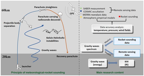
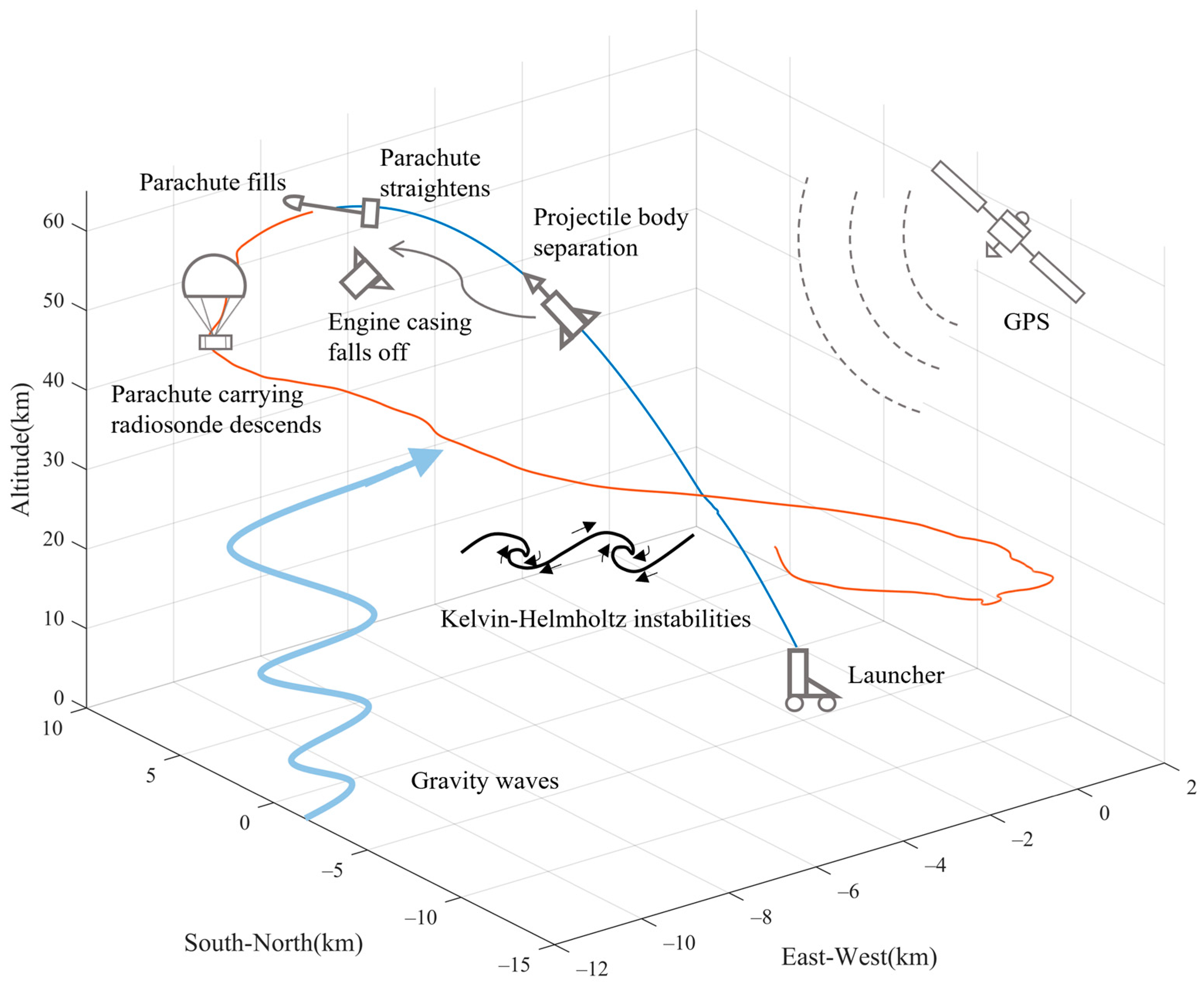
2.1. Detection Principle of the Meteorological Rocket

The meteorological rocket used here was launched over the East China Sea in December 2022. Figure 1 illustrates the detection trajectory during its ascending and descending phases, as well as the working principle of the meteorological rocket for atmospheric environment detection. Initially, the sonde was carried by the meteorological rocket to an altitude above 60 km. Then, the ejection separation system was activated, separating the sonde, recovery parachute, arrow cone, and the arrow-body-recovery module. Subsequently, the recovery parachute was gradually straightened under the guidance of the guide parachute, providing lift for the descent of the sonde.
During the experiment, temperature data were directly observed through the bead thermistor, and the position information (longitude, latitude, and altitude) of the rocket sonde was obtained through the navigation satellite system. The pressure at each altitude was calculated from the measured base pressure using the barometric height formula, and the atmospheric density was calculated using the ideal gas equation. For the preprocessing of temperature data and position data, coarse errors were eliminated by setting the threshold value using the 3 σ law and then using three Hermite interpolations to make up the points. Taking into account the pendulum period of the parachute, an integer multiple of the swing period as the smooth-fitting interval was used to smooth the data.
Due to the varying speed of the sonde during the descent, different numbers of points were used to fit the positional data at different altitudes. The first derivative of the linear fit was used to obtain the velocity, and the second derivative of the fourth-order fit was used to obtain the acceleration. Figure 2 shows the variation in velocity and acceleration with time during the descent of the rocket sonde. The data of the wind field during the descent of the sonde can be obtained by inverting the speed and acceleration [1]. When the speed and acceleration of the descent stage are determined, the wind speed can be calculated using the following formulas:
W x = x ˙ x ¨ z ¨ g z ˙
W y = y ˙ y ¨ z ¨ g z ˙
W = W x 2 + W y 2
where W x , W y , and W represent the meridional (north–south), zonal (east–west), and resultant wind speed, respectively. x ˙ , y ˙ , and z ˙ represent the velocity of the rocket sonde in the X , Y , and Z directions, respectively. x ¨ , y ¨ , and z ¨ represent the acceleration of the sounding instrument in the X , Y , and Z directions, respectively. g represents the gravitational acceleration at the launch site. Given the meridional and zonal wind speed, the wind direction θ can be calculated using the following formula:
θ = { arctan | W y W x | + 180 ° , ( W x > 0 , W y > 0 ) arctan | W y W x | + 180 ° , ( W x > 0 , W y < 0 ) arctan | W y W x | + 360 ° , ( W x < 0 , W y > 0 ) arctan | W y W x | , ( W x < 0 , W y < 0 )
The data sampling frequency was 2 Hz. Due to the varying descent speeds at different altitudes, the sampling interval initially started at several tens of meters and gradually decreased during the descent, reaching approximately 1~2 m at an altitude of 20 km.
In view of the correction of temperature data, the temperature measurement model given by the World Meteorological Organization (WMO) was used here for processing. The model is divided into the following terms: pneumatic heating, temperature hysteresis, direct solar radiation, short-wave radiation emitted by the earth’s surface and clouds, long-wave radiation, environmental thermal radiation, structural heat conduction, and measured current heating. The temperature profile was effectively corrected using this model.
In addition, four hours before the rocket launch, a sounding balloon was released to detect the atmosphere above the launch site. Figure 3 shows a comparison of the temperature, wind speed, and wind direction between the balloon detection and the rocket detection. It can be seen that the results are basically consistent.

2.2. Atmospheric Empirical Model

MSIS (Mass Spectrometer and Incoherent Scatter empirical model) is an empirical model widely used internationally to describe the atmospheric environment in the middle and upper atmospheres. It is based on data obtained from satellite mass spectrometers and ground-based incoherent scatter radars [27]. By inputting the location, time, solar activity, and geomagnetic activity, one can obtain the density, temperature, and other element profiles of the neutral atmosphere in the range of 0 to 1000 km altitude at the corresponding location.
HWM (Horizontal neutral Wind Model) builds an empirical model of the atmospheric wind field from the ground to the upper atmosphere (0~500 km) based on decades of data from rockets, satellites, and ground-based observation devices, combined with a spherical harmonic-function-fitting equation [28]. The results of the mean wind field at this location can be obtained by inputting information on elements such as position, time, and geomagnetic activity. The latest version of HWM, HWM07, is used in this paper.
MSIS and HWM have a low vertical resolution of 0.5 km. This study only compares the altitude range that matches the rocket’s detection range.

2.3. Satellite Remote-Sensing Data

The TIMED satellite was launched from Vandenberg Air Force Base in the United States in December 2001. It is a quasi-sun-synchronous satellite used to detect atmospheric temperature, pressure, wind field, chemical composition, and energy transport from the mesosphere to the lower thermosphere region [4]. The Sounding of the Atmosphere using Broadband Emission Radiometry (SABER) instrument on the TIMED satellite is a broadband radiometer that observes atmospheric infrared emissions in limb-viewing geometry with an altitude resolution of about 2 km [29]. By measuring the infrared radiation of Earth’s atmosphere at the limb, it provides information on the atmospheric temperature and basic composition from the lower stratosphere to the lower thermosphere. Under normal observation conditions, approximately 1400 atmospheric profiles can be obtained daily, with a horizontal resolution of about 400 km. The temperature error is 1–3 K in the 15–80 km altitude range [5,30]. The data used in the paper is Version v2.0 of SABER/TIMED, which includes temperature, water vapor, ozone, and other atmospheric information.
COSMIC (Constellation Observing System for Meteorology, Ionosphere, and Climate) is a collaborative research project between the United States and Taiwan, China. The COSMIC constellation consists of 6 identical microsatellites, each carrying a GPS Occultation Experiment (GOX) receiver to conduct radio-occultation observations of the Earth’s atmosphere [31]. The COSMIC occultation data provides global coverage and is designed to offer 2500 atmospheric profiles per day, with a vertical resolution of approximately 0.5–1.5 km and a horizontal resolution of around 200–300 km. We used the level 2 “atmPrf” version of the COSMIC data, which can provide dry-temperature profiles from the surface up to 60 km altitude [32].

2.4. MERRA-2 Reanalysis Dataset

MERRA (Modern-Era Retrospective analysis for Research and Applications) is a global climate reanalysis dataset developed and maintained by the National Aeronautics and Space Administration (NASA) of the United States. MERRA-2 is produced by the 5.12.4 version of the GEOS atmospheric data assimilation system with the GEOS atmospheric model and GSI analysis scheme as the core [33]. Compared with the previous version of MERRA reanalysis data, MERRA-2 uses a cubed-sphere grid to reduce the grid-spacing singularities on the latitude–longitude grid, assimilate more satellite observation data, reduce the deviation of the water cycle, show more accurate zonal wind and mean meridional circulation, and provide atmospheric-aerosol reanalysis data [33,34,35]. In this study, the MERRA reanalysis wind-field data used in this paper has a temporal resolution of 3 h, a horizontal resolution of 0.625° × 0.5°, and a total of 72 vertical layers from the ground level to an altitude of 78 km.

2.5. Data Comparison Method

During the comparative analysis, due to the multiple sources and varying accuracy of the data, the rocket-sounding dataset with the highest vertical accuracy was interpolated to match the altitude values of the other datasets. When analyzing the variability of the temperature elements, the deviation E , maximum deviation E max , mean deviation E ¯ , average deviation rate R ¯ , and R M S were calculated. The calculation formulas for these are as follows:
E i = X i X 0 i
E max = max ( a b s ( E i ) )
E ¯ = 1 N i = 1 N a b s ( E i )
R ¯ = 1 N i = 1 N | X i X 0 i X 0 i |
R M S = i = 1 N ( X i X 0 i ) 2 N
where X 0 i refers to the data obtained from rocket observations at a particular point, X i represents the values of satellite observations or model data at a specific altitude, and N is the total number of data points.
When analyzing the differences in pressure, it is more reasonable to calculate the deviation rate R i between different datasets, because pressure changes exponentially with altitude.
R i = X i X 0 i X 0 i

2.6. Gravity-Wave Power–Frequency Spectrum

Wind shear is an important factor in the generation of gravity waves, and changes in the wind and temperature fields are a key manifestation of gravity waves [2,36,37,38]. In order to analyze the different gravity-wave parameters extracted by different detectors, gravity-wave spectra were extracted from the wind shear and wind-field profiles detected by the rocket and the temperature profiles of satellite data, respectively. For the wind-field and temperature profiles, the original profiles were subtracted from the background profiles to obtain the perturbation profiles, using a fourth-order polynomial fit as the background profile. With regard to wind shear, a high-pass filter with a cutoff wavelength of 20 km was applied to obtain the profiles considered to be perturbations caused by gravity waves. Subsequently, gravity-wave spectra were extracted from the perturbation profiles using the maximum-entropy method. Different types of data were interpolated into the profiles with a 1 km interval to extract the gravity-wave power–frequency spectra.
Compared with general spectral analysis methods, the MaxEnt (Maximum Entropy) spectral analysis shows a better ability to estimate the signal’s spectrum using the maximum-entropy principle with limited information, along with good spectral resolution and noise robustness, which is suitable for the rocket’s wind-field data. By solving the Yule–Walker equation and obtaining the model parameters, the signal’s power spectrum can be estimated using the following equation:
P ( e j ω ) = δ ω 2 | 1 + k = 1 N a k e j ω k |
P ( e j ω ) represents the power spectral density of a complex exponential signal with a frequency of ω . δ ω represents the frequency-resolution window. N is the polynomial order, which determines the frequency range and complexity of the signal fitting. a k represents the complex coefficients of the polynomial.

2.7. Kelvin–Helmholtz Instability

Wind shear refers to the sudden change in wind speed and wind direction in the atmosphere. Wind shear often occurs in regions with high wind speed and is closely related to the existence of jet streams [39]. The formula for calculating the intensity of vertical wind shear is expressed as follows:
d U d z = ( d u d z ) 2 + ( d v d z ) 2
In the formula, u and v represent the meridional wind and zonal wind, respectively, while z represents the altitude. The derivatives d u d z and d v d z were calculated using the central-difference method. Here, the rocket-sounding data were interpolated uniformly at 50 m intervals. Taking into account small-scale perturbations and data jitter caused by noise, a 1 km sliding average of the wind shear was performed here [21].
The N (Brunt–Väisälä) frequency is an important parameter that describes vertical oscillations and stability in the atmosphere. It characterizes the stability of vertical oscillations in the atmosphere. N 2 can be used to determine the stability of the atmospheric stratification. When N 2 > 0 , the basic stratification is considered stable. The expression for N 2 is as follows:
N 2 = g T ( d T d z + g c p )
In the formula, g and c p represent the acceleration of gravity and the specific heat at constant pressure, respectively. T represents temperature, and z represents altitude. In order to eliminate the influence of vertical disturbance on the buoyancy frequency, we calculated a five-point sliding average of the frequency (corresponding to a smooth window of 200 m).
Subsequently, the obtained wind shear and buoyancy frequency can be used to calculate the Richardson number. The Richardson number is a dimensionless parameter. When it is below a critical value (typically 0.25), the atmospheric condition in that region is considered unstable, indicating the potential occurrence of KHI. The equation for the Richardson number is as follows:
R i = N 2 ( d u d z ) 2 + ( d v d z ) 2

2.8. Gravity-Wave Energy

The original profiles of wind field and temperature were fitted using a fourth-order polynomial to obtain the background profiles. Then, a high-pass filter with a cutoff wavelength of 20 km was applied to the perturbation profiles obtained by subtracting the background profiles from the original profiles. The remaining perturbations were considered as disturbances caused by gravity waves. The total energy of gravity waves E t was calculated from the meridional wind perturbation ( v ), zonal wind perturbation ( u ), and temperature perturbation ( T ) according to the following formula:
E t = E k + E p
E k = 1 2 [ u 2 ¯ + v 2 ¯ ]
E p = 1 2 ( g N ) 2 ( T T ¯ ) 2
where T T ¯ represents the normalized temperature disturbance. E k and E p represent the kinetic energy and potential energy per unit mass, respectively. u ¯ and v ¯ represent the average values of wind-speed disturbances within a certain interval range. Due to the limited availability of one-time sounding data in this study, the strength of the gravity-wave activity was assessed by computing the vertical profile of the gravity-wave energy. In order to calculate the gravity-wave energy and the Richardson number (Ri), the wind-field components u and v were interpolated at 50 m intervals.

3. Results

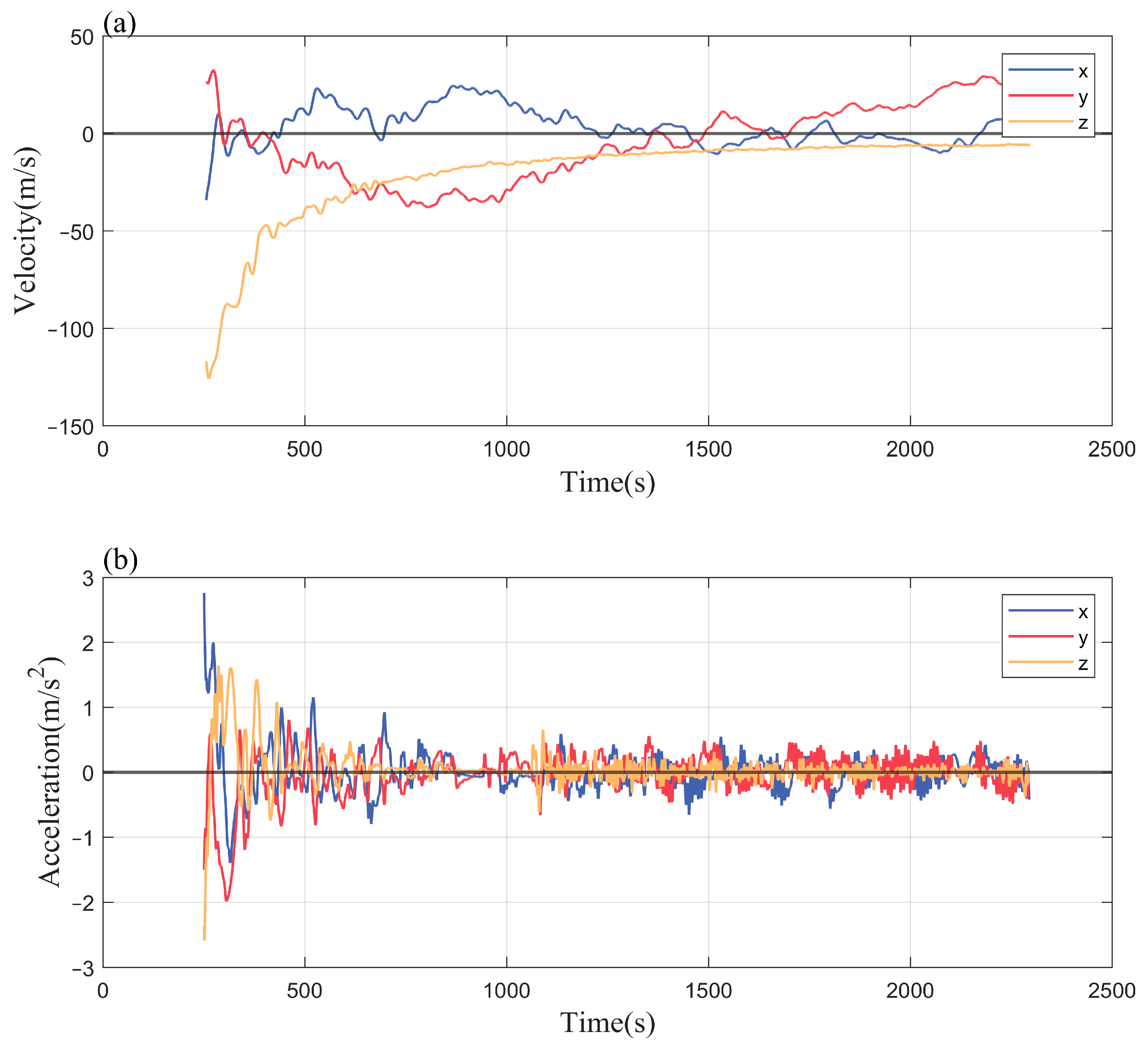
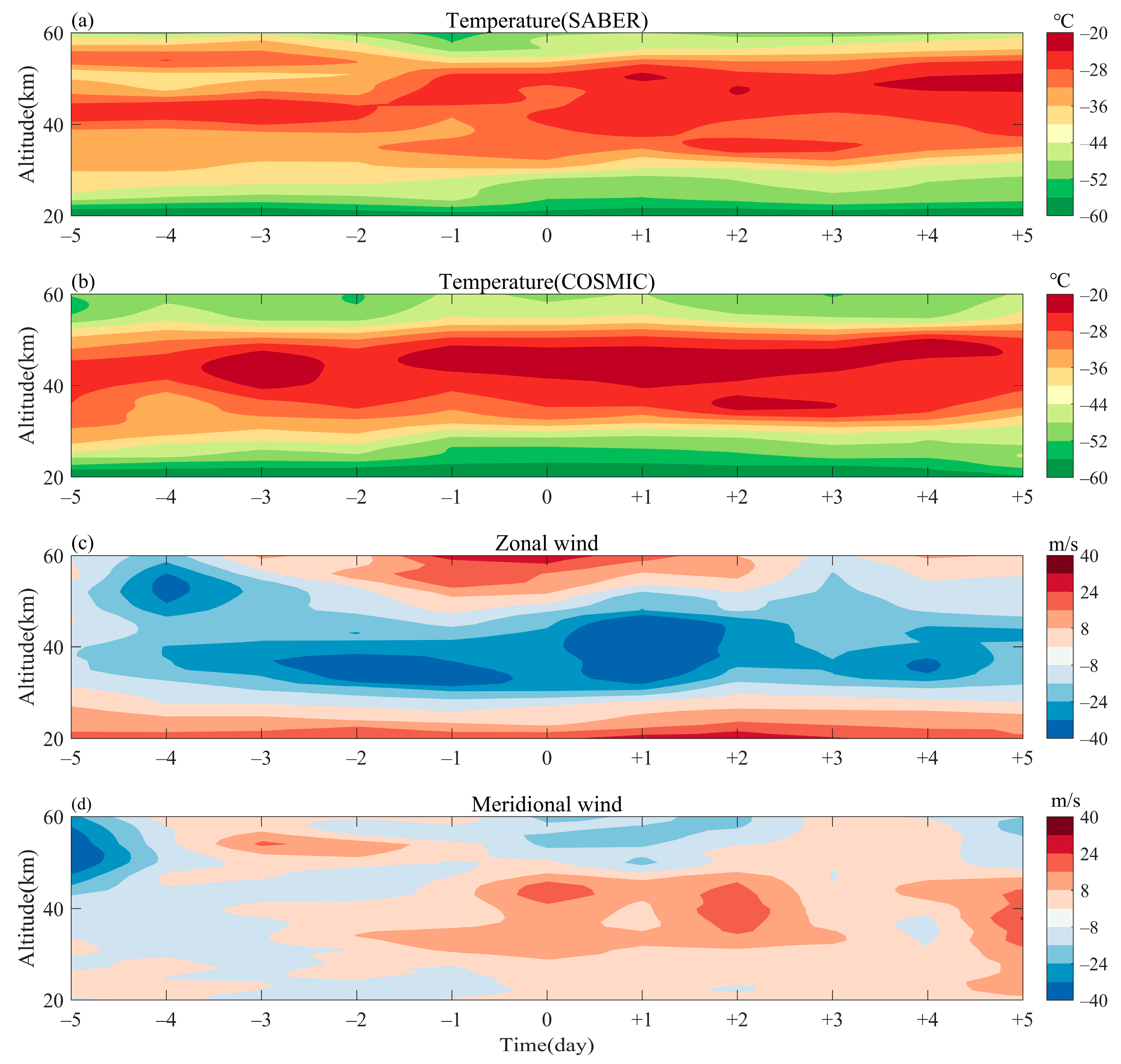
3.1. Time-Series Analysis of Temperature and Wind-Field Profiles

Figure 4 depicts the variations in temperature with altitude and time at the rocket launch site spanning the five days prior to and the five days after the rocket launch, using COSMIC and SABER data. It also illustrates the changes in zonal and meridional winds with altitude and time at the launch site using reanalyzed MERRA-2 data. When studying the temperature variation with altitude and time, the average of all temperature profiles within ±5° of the latitude and longitude range over the launch site was considered the satellite temperature observation of that day over the rocket launch site. Considering the uniform spatial resolution and high accuracy of the MERRA-2 reanalysis data, the profiles closest to the launch site and that had the time closest to the local time of the launch day were selected. In total, we considered data for 11 days, including five days before and after the rocket launch, to assess if the local wind-field background was not a state of abrupt change.
From Figure 4a,b, it can be seen that in the altitude range of 20~30 km, the temperatures observed by COSMIC are lower than those observed by SABER, while in the altitude range of 30~50 km, the temperatures observed by SABER are lower than those observed by COSMIC. The temperature distribution between the two observation profiles exhibited different trends before two days prior to the rocket launch. However, they become consistent one day after the rocket launch. In the distribution of the wind field, it is observed that the meridional wind speed is generally significantly lower than the zonal wind speed. From Figure 4c, it can be seen that there is little variation in the zonal wind speed in the two days before and after the rocket launch. At altitudes of 20–30 km, there was a westerly wind, while at around 30–50 km, there was an easterly wind followed by a return to a westerly wind. In terms of the distribution of the meridional wind, it can be found from Figure 4d that the stratospheric meridional wind changed from north to south two days before the launch of the rocket and maintained a large southerly wind speed. Therefore, it can be concluded that the atmospheric element distribution on the launch day is relatively stable, and the comparative analysis of different datasets will not be biased by sudden changes in atmospheric elements occurring at the time of launch.

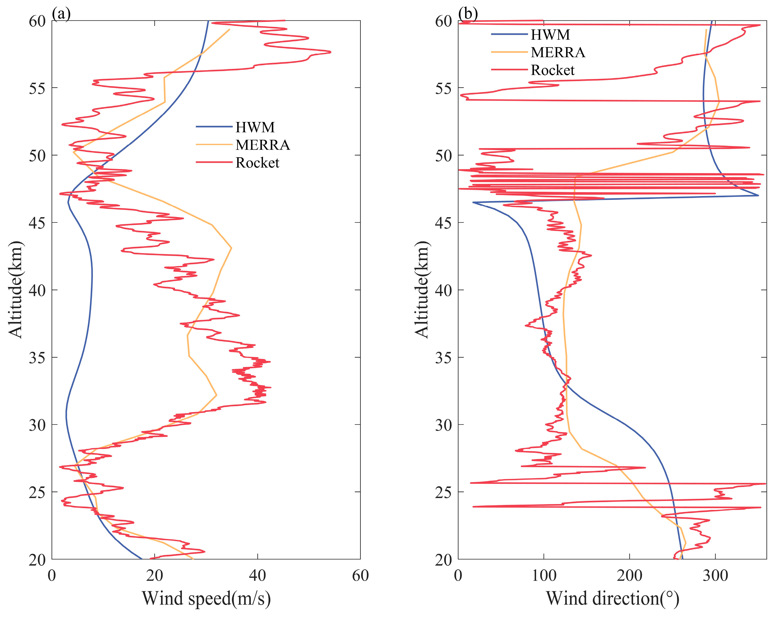
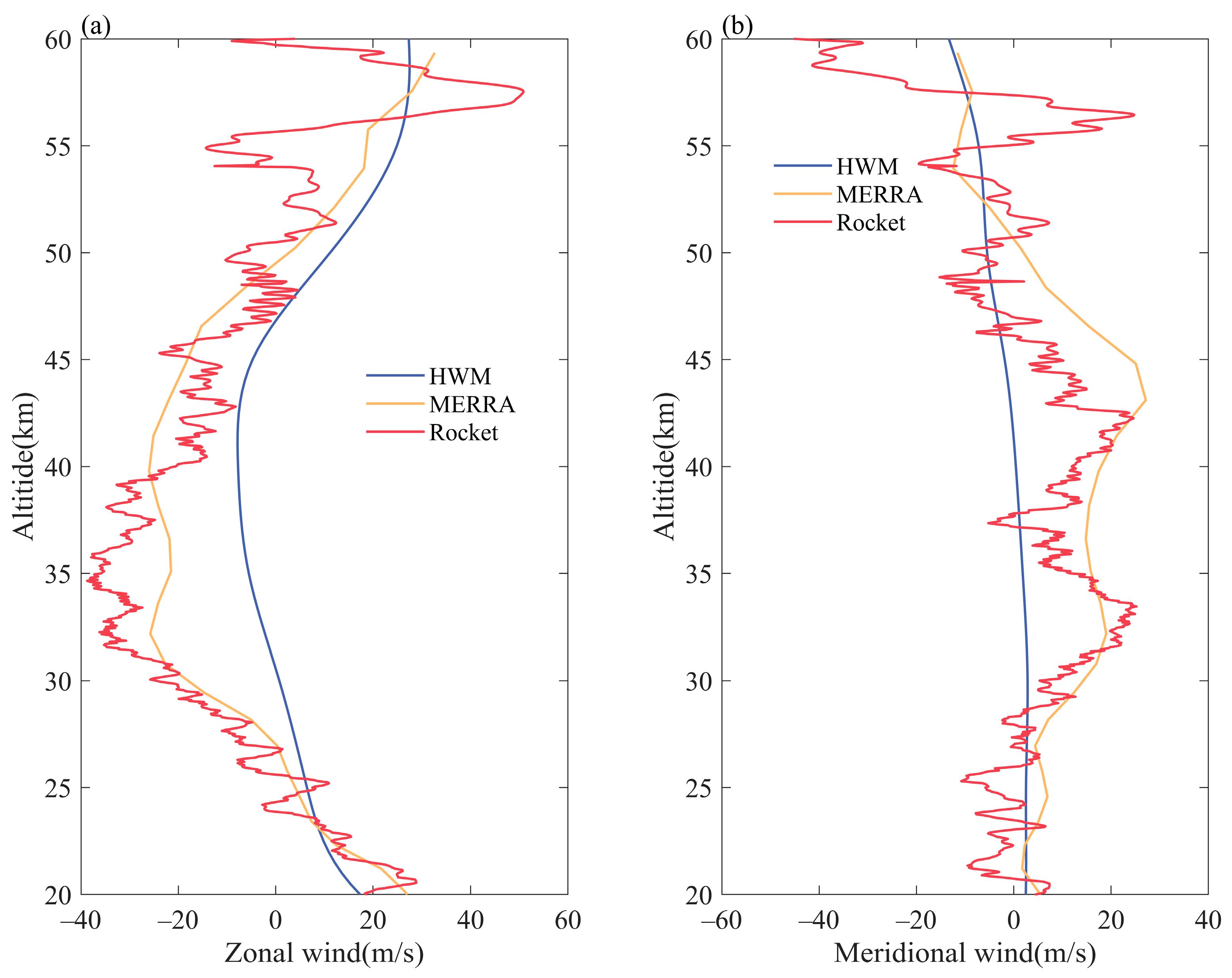
3.2. Comparison of Temperature, Pressure and Wind-Field Data

By inputting the location information and time of the rocket launch site, the atmospheric temperature and density information from the MSIS model under the same conditions can be obtained, and the pressure can be calculated through the barometric-height formula. The observational data from the SABER and COSMIC systems that were close to the rocket launch site on the same day were searched, and the corresponding temperature and pressure profiles with altitude variations were obtained.
The temperature comparison between the rocket, remote sensing, and MSIS is shown in Figure 5. From Figure 5a, it can be seen that the temperature distribution trends of the different data are basically the same, and there is not much difference between the rocket-sounding data and the remote-sensing observation and atmospheric model, indicating that the rocket-sounding dataset has good credibility and can better reflect the distribution of local atmospheric elements. If the occurrence of the maximum temperature is considered to be the height of the stratopause, the altitude of the stratopause observed by the rocket is roughly 47 km, which is not very different from the stratopause shown by the MSIS model and COSMIC data. However, SABER observed a temperature maximum at around 37 km, followed by a decrease in temperature with increasing altitude but a lower rate of temperature decreases at 45~50 km, where the inversion occurs again. In the distribution of temperature deviations, it can be seen that below 40 km, the COSMIC data and MSIS model data show lower values. But above 40 km, the difference between the COSMIC data and the rocket probe data becomes larger. This may be due to the increasing contribution of the ionosphere’s bending effect on electromagnetic waves at higher altitudes. Even after ionospheric correction, residual errors that cannot be eliminated may still exist, leading to significant observational noise and reduced accuracy in the inversion of atmospheric parameters [40].
Table 1 presents the statistical comparisons of the rocket-sounding data with the satellite data and MSIS. The average deviations between the COSMIC occultation data, SABER data, MSIS model data, and rocket-sounding temperature data are 3.34 °C, 5.38 °C, and 5.38 °C, respectively. The root mean-square errors are 3.9 °C, 6.8 °C, and 6.4 °C, respectively. The trend distribution of the COSMIC occultation data shows the closest agreement with the rocket-sounding data and has the smallest deviation. Although the average error of SABER data and MSIS data is the same compared to rocket-sounding data, the error rate and root mean-square error of SABER data are greater, indicating that the degree of deviation of SABER data from rocket data has changed. As can be seen from Figure 5, SABER has a systematic negative deviation above 40 km altitude, and this tends to increase with height.
The comparison of the rocket, satellite, and MSIS model pressure data is shown in Figure 6. Below 30 km, the satellite and MSIS data are dominated by small positive deviations; above 45 km, the deviation of the SABER measurements increases rapidly, while the deviation of the MSIS model data and COSMIC measurements is always within 5%.
Overall, the COSMIC occultation data show the smallest deviation compared with the rocket-sounding data, followed by MSIS model data, and the SABER data show the largest deviation. The deviation between the rocket data and the MSIS model can be attributed to a few factors. Firstly, the MSIS model is an empirical model based on long-term averages with low spatiotemporal resolution. Secondly, when the MSIS model was developed, there was a lack of sounding data for the stratosphere in the Chinese region, leading to inaccurate descriptions. Regarding the deviation between the rocket data and the satellite data, the larger deviation in the SABER data compared with the COSMIC data can be attributed to two reasons. Firstly, there are differences in the timing and spatial coverage of the individual profile measurements. Secondly, due to differences in their satellite-observation principles, COSMIC observation has a higher temporal and spatial resolution compared with SABER observation. COSMIC data is currently considered to be relatively accurate below 40 km, but as the altitude increases, the influence of the ionosphere becomes more significant, leading to a decrease in detection accuracy [41]. Some studies have been conducted to analyze the accuracy of COSMIC occultation data, and through radiosondes, it has been verified that COSIMC occultation data is unbiased in the lower stratosphere region [42,43]. Below 40 km, the temperature deviation is negative, and there is a relatively uniform systematic error, but above 40 km this systematic error is not obvious. In terms of air-pressure comparison, the deviation below 40 km is relatively small, and the deviation above 40 km tends to increase as the height increases. There are also studies indicating that SABER/TIMED data exhibit systematic bias below 70 km, with a large negative bias in upper stratospheric temperatures [44], which is consistent with the conclusions drawn in our paper. Fan et al. [45] pointed out that within a given range of consistent time and space, the temperature observations from SABER and COSMIC data in the winter of the Chinese region show little difference below 40 km, with primarily negative deviations observed at 40~60 km heights reaching a maximum of −6 K. This is consistent with the deviation trends of the selected satellite data in this study.
By inputting the location and time information of the rocket launch site, wind-field data from the HWM model can be obtained. Similarly, wind-field data from the nearest location and time in the MERRA reanalysis dataset was selected. The MERRA-2 data matched the launch position, and the time of the rocket differed by less than 0.5 degrees in latitude and longitude and less than 1.5 h in time. After obtaining the wind speed of the meridional and zonal wind under the same conditions as the rocket launch site, the total wind speed and direction were calculated by Equations (3) and (4).
Figure 7 shows the comparison of the wind speed and direction of the rocket with the HWM model and the MERRA reanalysis data. Figure 8 compares the zonal and meridional wind speed. It can be clearly seen that, in terms of wind speed, the MERRA reanalysis data is more consistent with the observed trend from the rocket data, while the HWM model shows significant differences from the rocket-detected wind speeds. In terms of wind direction, the different datasets exhibit similar distribution trends with height, indicating the reliability of the rocket-sounding data. At altitudes between 30~45 km, the wind speed from the HWM model is noticeably lower. This is primarily due to the model’s underestimation of the zonal and meridional wind in this altitude range, particularly in describing the eastward jet. Moreover, in the altitude range of 50~60 km in the mesosphere, the model wind field and reanalysis wind field also have a large deviation from the rocket-detection wind field. The unrealistic features observed at the upper model levels are attributed, in part, to the inherent damping effect on the reanalysis data [29]. Similar conclusions were drawn by Z. Sheng et al. [14] through comparing rocket data with both the WACCM model and HWM model wind fields. The differences between the MERRA reanalysis wind field and the rocket-detected wind field can be attributed to a few factors. Firstly, the MERRA reanalysis data is a result of assimilating multiple observational datasets, whereas a single rocket measurement is subject to various influencing factors. Secondly, the vertical resolution of the MERRA reanalysis data is relatively low and decreases with increasing altitude. Therefore, it is normal to observe differences between the reanalysis data and rocket-detected wind fields in the mesosphere.
Here, for the analysis of the wind field, the rocket-sounding data is more capable of describing the fine structure of the atmospheric wind field, and the fluctuation and wind shear are more pronounced. At the 25 km and 47 km altitudes, there are significant persistent oscillations in wind direction. It is noteworthy that these two altitude layers are near the height of zero zonal wind speed and are the transition layers of the wind direction changing from west (east) to east (west), and the overall wind speed is low. Once there are fluctuations in wind speed, the wind direction also fluctuates significantly. Considering the high resolution of the rocket sounding, it is reasonable to observe rapid changes in wind direction at these altitude layers.

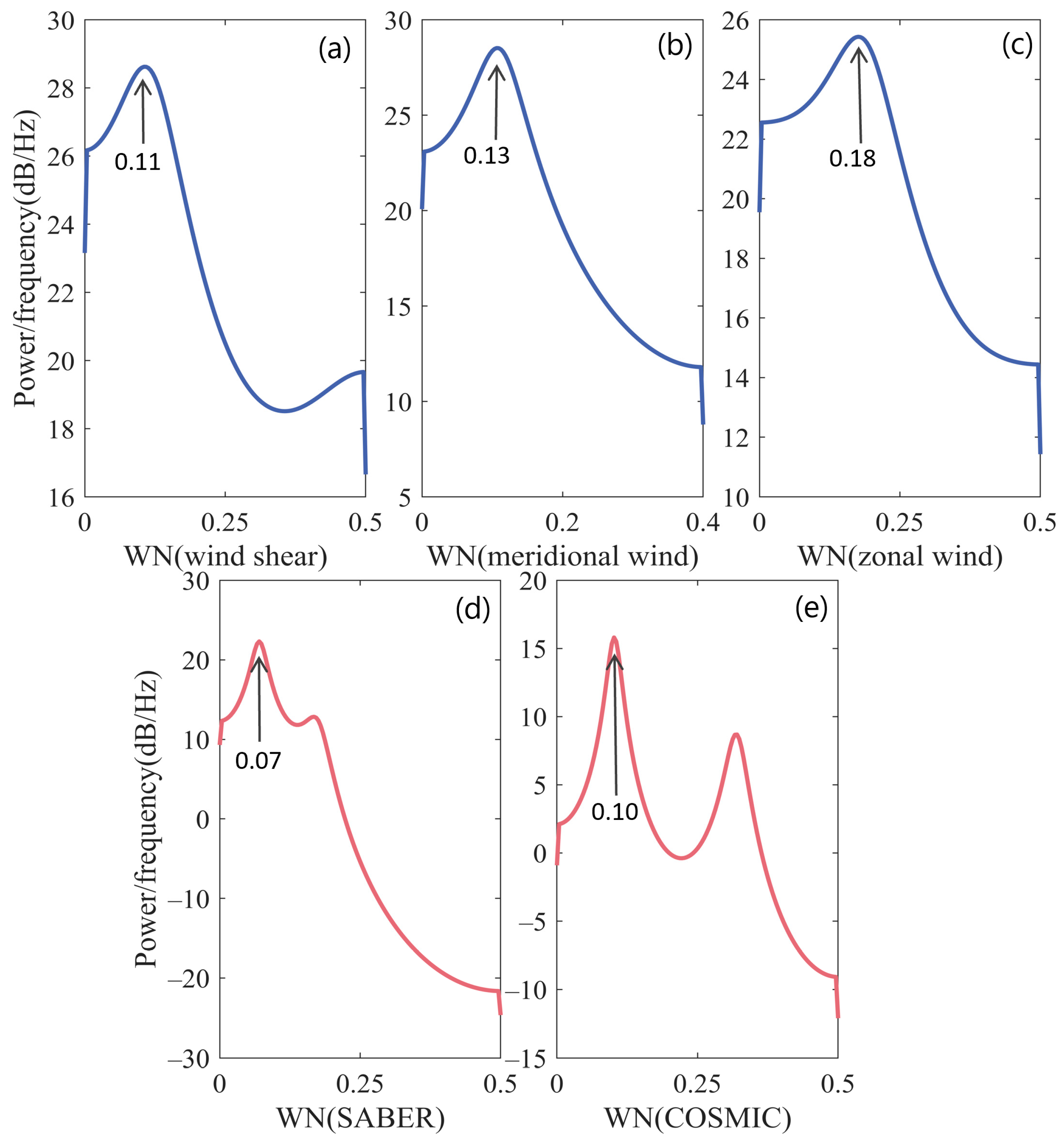
3.3. Atmospheric Gravity-Wave Spectrum Analysis

Figure 9 shows the gravity-wave power–frequency spectra obtained from rocket detection profiles and remote-sensing detection profiles using the maximum-entropy method. Figure 9a–c respectively show the gravity-wave spectra extracted from the wind shear, zonal wind, and meridional wind obtained from rocket detection, with main wavelengths of 9.1 km, 7.7 km, and 5.6 km. Figure 9d,e respectively show the gravity-wave spectra extracted from temperature profiles observed by COSMIC occultation and SABER, with main wavelengths of 14 km and 10 km. The gravity-wave wavelengths extracted from remote-sensing observations are significantly larger than those obtained from rocket-detection profiles. Due to the wide range of gravity-wave scales, each observation instrument can only observe a specific part of the gravity-wave spectrum [46]. Therefore, such differences are most likely caused by the lower resolution of satellite remote-sensing detection, and the vertical resolution of COSMIC occultation observation is higher than that of SABER observation, resulting in shorter extracted wavelengths.

3.4. The Interrelationship between KHI and the Gravity-Wave Energy

From Figure 10a, it can be observed that the wind shear remains relatively stable below 40 km, but at altitudes between 40 km and 48 km, the wind shear increases with altitude. In Figure 10b, it can be noted that all N 2 values are positive, indicating a generally stable atmosphere over the launch site. However, there are significant fluctuations in N 2 values in the altitude range of 45 km to 50 km, followed by a decrease. This corresponds precisely to the rapid increase in wind shear, suggesting the possible presence of a turbulent layer in this altitude range.
The occurrence of KHI is primarily measured by a critical value of the Richardson number (Ri) being below a certain threshold [47]. Figure 10e illustrates the vertical distribution of Ri. It can be observed that there are continuous altitude layers with Ri values below 0.25 in the height ranges of 53~57 km, 47~49 km, and 26~27 km. In the height ranges of 37~40 km and 23~26 km, there are discontinuous atmospheric layers with Ri values below 0.25. In other words, KHI mainly occurs in these five regions. By comparison with Figure 10a, it can be noticed that the regions where KHI occurs align with areas of a sudden increase in wind shear. This is also consistent with previous studies, as KHI often develops in regions of strong shear flow [25,48].
From Figure 10c,d, it can be inferred that below an altitude of 40 km, there exists a clear proportionality between the total energy and the potential energy of gravity waves. However, above 40 km, the proportionality relationship between the total energy and the potential energy of gravity waves becomes less evident. Above 40 km, wind shear gradually increases with altitude, which may trigger the generation of gravity waves at different scales. Furthermore, the background wind-field transitions from easterly to westerly, and this change in the background wind field can also impact the propagation and development of gravity waves [49,50]. These factors collectively contribute to the complexity of the proportionality relationship between potential energy and total energy in the context of gravity-wave dynamics. The five regions in which KHI is predominantly observed have been identified and correspond to the peaks in gravity-wave energy, particularly in the potential energy peak, which is observed to occur in KHI regions. The gravity waves and KHI are closely linked through complex dynamic processes, playing an important role in the transfer of energy and momentum in the atmosphere [26,47,51,52]. KHI occurs at the interface of two fluids with different densities, giving rise to instability due to variations in fluid velocity and density. This instability can lead to the generation of waves, subsequently giving rise to gravity waves [23]. The process of KHI-induced gravity-wave generation has been described, wherein KHI manifests as an unstable billow motion that forms periodic vortex structures [23,53]. Meanwhile, research has also shown that gravity waves can serve as a triggering mechanism for KHI. This is because the presence of gravity waves in fluid layers with varying atmospheric densities can lead to the generation and intensification of wind shear, which, in turn, triggers the instability at the fluid interface and gives rise to KHI [25]. Because individual gravity waves do not exist in the actual atmosphere, multiple gravity waves are often superimposed, making it impossible to determine which one is the excitation source in the study. However, direct observation has shown a strong connection between the occurrence of KHI and gravity-wave energy in the stratosphere and lower mesosphere. This serves as important evidence of the interaction between KHI and gravity waves.

4. Discussion

This article focuses on the principles of meteorological-rocket detection and its data-processing procedures, which will be very helpful for those who want to understand the principles of meteorological-rocket detection or who need to process meteorological-rocket data. Based on the comparison and analysis of rocket data with various widely used datasets, the accuracy of rocket data has been verified and validated. The obtained results are generally consistent with previous studies, showing that COSMIC data are relatively accurate below 40 km, while SABER data exhibit a systematic negative bias above 40 km. Previous studies have often used cross-validation of satellite data or radiosonde at altitudes below the stratosphere [41], while this article provides a higher level of credibility by analyzing the accuracy of different datasets based on in situ detection at altitudes of 20–60 km. This study only utilized data from a single rocket experiment. The findings of this study can serve as a reference for future research using the data compared in this study. However, to understand the differences in these data at different times, more rocket experiment data would be required.
This study analyzes the relationship between gravity-wave activity and KHI by calculating the gravity-wave energy and Richardson number. The research shows that the peak energy of gravity waves corresponds well with the regions where KHI occurs, providing direct observational evidence of the interaction between gravity waves and KHI. Currently, due to the lack of abundant detection methods for the middle atmosphere, studies on middle atmospheric dynamics often rely on limited direct observations and numerical simulations [25,54,55]. In many numerical simulations, one of the processes is usually treated as the excitation source. However, in this study, we were unable to analyze the underlying mechanism of how this occurs or determine causality, and we could only observe the consistency between the high energy of gravity waves and the occurrence of KHI.
Gravity waves and KHI are important dynamical processes in the middle atmosphere, playing a crucial role in the transfer of energy and distribution of substances in the atmosphere [46]. One important future research direction is to conduct small-scale dynamic experiments in the middle atmosphere based on direct observations. The results of this study are expected to provide useful feedback for the use of meteorological-rocket data and research on middle-atmospheric dynamics.

5. Conclusions

This study introduces the detection principle and data-processing process of a meteorological rocket launched over the East China Sea. Based on the comparison of rocket data, the deviation between different datasets and rocket data was analyzed, the gravity-wave parameters were extracted, and the atmospheric dynamic stability over the launch site was analyzed. The primary findings can be summarized as follows:
(1) Rocket-sounding data offers a reliable representation of atmospheric elements and the vertical distribution of wind fields. The data obtained through this method is highly credible and has high resolution, enabling a more detailed characterization of the atmosphere. Compared with the temperature data observed by the rocket, COSMIC data exhibited a better overall agreement with the rocket observation, while SABER data showed the largest deviation. Regarding wind-field data, the wind field detected by the rocket aligned with the MERRA reanalysis wind-field trend, albeit exhibiting finer changes in the wind field. This study also examines the factors contributing to the varying levels of accuracy in different datasets.
(2) In this study, gravity-wave wavelengths were extracted from the wind shear, meridional wind, and zonal wind profiles obtained by rocket measurements using the maximum-entropy method, and they were found to be 9.1 km, 7.7 km, and 5.6 km, respectively. Subsequently, gravity-wave wavelengths were extracted from various remote-sensing data, including SABER and COSMIC temperature profiles, yielding values of 14 km and 10 km. In comparison with satellite data, rocket observation enables the extraction of gravity-wave parameters with a higher resolution and enables the detection of more intricate gravity-wave structures.
(3) By utilizing calculated wind shear and N 2 profiles, we computed the Richardson number (Ri) and observed that regions of rapid wind-shear increase corresponded to the occurrence of KHI. The computation of gravity-wave energy was conducted to analyze the relationship between KHI and gravity waves. The results revealed that in all five regions where KHI occurred, there were corresponding peaks in the gravity-wave energy, particularly in relation to potential energy. In this study, direct observation demonstrated a clear mutual interaction between KHI and gravity waves in the middle atmosphere.

Author Contributions

Conceptualization, Y.S. and Y.H.; methodology, Y.S.; validation, Y.S. and H.L.; formal analysis, Y.S., Y.H. and H.L.; investigation, Y.S.; resources, Y.H.; visualization H.L.; writing—original draft preparation, Y.S.; writing—review and editing, Y.H.; supervision, Y.H.; project administration, Y.H.; funding acquisition, Y.H. All authors have read and agreed to the published version of the manuscript.

Funding

This research was supported by the National Natural Science Foundation of China (grant number 42275060), the Hunan Outstanding Youth Fund Project (grant number 2021JJ10048), and the Postgraduate Scientific Research Innovation Project of Hunan Province (grant number CX20220046).

Data Availability Statement

The SABER data utilized in this work is openly available at: https://saber.gats-inc.com (accessed on 17 February 2023) The MERRA-2 reanalysis dataset utilized in this work is openly available at: https://gmao.gsfc.nasa.gov/reanalysis/MERRA-2 (accessed on 22 March 2023). The COSMIC occultation data utilized in this work is openly available at: https://cdaac-www.cosmic.ucar.edu (accessed on 9 March 2023).

Acknowledgments

The authors are thankful for the support provided by the “Western Light” Cross-Team Project of the Chinese Academy of Sciences, Key Laboratory Cooperative Research Project. Additionally, helpful comments by the editors and the specific anonymous reviewer are gratefully acknowledged.

Conflicts of Interest

The authors declare no conflicts of interest.

References

  1. Fan, Z.; Sheng, Z.; Wan, L.; Shi, H.; Jiang, Y. Comprehensive assessment of the accuracy of the data from near space meteorological rocket sounding. J. Appl. Meteorol. Climatol. 2013, 62, 199601. [Google Scholar] [CrossRef]
  2. He, Y.; Zhu, X.; Sheng, Z.; Zhang, J.; Zhou, L.; He, M. Statistical Characteristics of Inertial Gravity Waves Over a Tropical Station in the Western Pacific Based on High-Resolution GPS Radiosonde Soundings. J. Geophys. Res. Atmos. 2021, 126, e2021JD034719. [Google Scholar] [CrossRef]
  3. Huang, K.M.; Yang, Z.X.; Wang, R.; Zhang, S.D.; Huang, C.M.; Yi, F.; Hu, F. A Statistical Study of Inertia Gravity Waves in the Lower Stratosphere Over the Arctic Region Based on Radiosonde Observations. J. Geophys. Res. Atmos. 2018, 123, 4958–4976. [Google Scholar] [CrossRef]
  4. Zhang, Y.; Xiong, J.; Liu, L.; Wan, W. A global morphology of gravity wave activity in the stratosphere revealed by the 8-year SABER/TIMED data. J. Geophys. Res. Atmos. 2012, 117, D21101. [Google Scholar] [CrossRef]
  5. Ern, M.; Trinh, Q.T.; Preusse, P.; Gille, J.C.; Mlynczak, M.G.; Russell, J.M., III; Riese, M. GRACILE: A comprehensive climatology of atmospheric gravity wave parameters based on satellite limb soundings. Earth Syst. Sci. Data 2018, 10, 857–892. [Google Scholar] [CrossRef]
  6. Kaifler, N.; Kaifler, B.; Dörnbrack, A.; Rapp, M.; Hormaechea, J.L.; de la Torre, A. Lidar observations of large-amplitude mountain waves in the stratosphere above Tierra del Fuego, Argentina. Sci. Rep. 2020, 10, 14529. [Google Scholar] [CrossRef]
  7. Banyard, T.P.; Wright, C.J.; Hindley, N.P.; Halloran, G.; Krisch, I.; Kaifler, B.; Hoffmann, L. Atmospheric Gravity Waves in Aeolus Wind Lidar Observations. Geophys. Res. Lett. 2021, 48, e2021GL092756. [Google Scholar] [CrossRef]
  8. Yang, W.Y.J.; Guo, W.; Yang, X.; Xia, Z.; Zhang, B.; Cheng, X.; Hu, X. Global Stratopheric Gravity Wave Characteristics by Aura/MLS and TIMED/SABER Observation Data. Chin. J. Space Sci. 2022, 42, 919–926. [Google Scholar] [CrossRef]
  9. Eckermann, S.D.; Hirota, I.; Hocking, W.K. Gravity wave and equatorial wave morphology of the stratosphere derived from long-term rocket soundings. Q. J. R. Meteorol. Soc. 1995, 121, 149–186. [Google Scholar] [CrossRef]
  10. Sun, Y.C.S.; Shao, S.; Cai, J.; He, Y.; Wang, F.; Shi, H. Method for Evaluation Uncertainty of Wind Measurements for Mete-orological Sounding Rocket. Meteorol. Sci. Technol. 2021, 49, 174–183. [Google Scholar] [CrossRef]
  11. Zhou, L.; Sheng, Z.; Fan, Z.; Liao, Q. Data Analysis of the TK-1G Sounding Rocket Installed with a Satellite Navigation System. Atmosphere 2017, 8, 199. [Google Scholar] [CrossRef]
  12. Millet, C.; Robinet, J.C.; Roblin, C. On using computational aeroacoustics for long-range propagation of infrasounds in realistic atmospheres. Geophys. Res. Lett. 2007, 34, L14814. [Google Scholar] [CrossRef]
  13. Friedrich, M.; Torkar, K.M.; Singer, W.; Strelnikova, I.; Rapp, M.; Robertson, S. Signatures of mesospheric particles in ionospheric data. Ann. Geophys. 2009, 27, 823–829. [Google Scholar] [CrossRef]
  14. Sheng, Z.; Jiang, Y.; Wan, L.; Fan, Z. A Study of Atmospheric Temperature and Wind Profiles Obtained from Rocketsondes in the Chinese Midlatitude Region. J. Atmos. Ocean. Technol. 2015, 32, 722–735. [Google Scholar] [CrossRef]
  15. Ge, W.; Sheng, Z.; Zhang, Y.; Fan, Z.; Cao, Y.; Shi, W. The study of in situ wind and gravity wave determination by the first passive falling-sphere experiment in China’s northwest region. J. Atmos. Sol. Terr. Phys. 2019, 182, 130–137. [Google Scholar] [CrossRef]
  16. Sheng, Z.; Li, J.W.; Jiang, Y.; Zhou, S.D.; Shi, W.L. Characteristics of Stratospheric Winds over Jiuquan (41.1° N, 100.2° E) Using Rocketsonde Data in 1967–2004. J. Atmos. Ocean. Technol. 2017, 34, 657–667. [Google Scholar] [CrossRef]
  17. Jiang, G.; Xu, J.; Shi, D.; Wei, F.; Wang, L. Observations of the first meteorological rocket of the Meridian Space Weather Monitoring Project. Chin. Sci. Bull. 2011, 56, 2131–2137. [Google Scholar] [CrossRef]
  18. He, Y.; Zhu, X.; Sheng, Z.; He, M. Identification of stratospheric disturbance information in China based on round-trip intelligent sounding system. Atmos. Chem. Phys. 2023; EGUsphere [preprint]. [Google Scholar] [CrossRef]
  19. Zhang, C.; Zhang, J.; Xu, M.; Zhao, S.; Xia, X. Impacts of Stratospheric Polar Vortex Shift on the East Asian Trough. J. Clim. 2022, 35, 5605–5621. [Google Scholar] [CrossRef]
  20. Zhang, S.D.; Yi, F.; Huang, C.M.; Huang, K.M. High vertical resolution analyses of gravity waves and turbulence at a midlatitude station. J. Geophys. Res. Atmos. 2012, 117, D02103. [Google Scholar] [CrossRef]
  21. He, Y.; Sheng, Z.; He, M. The Interaction Between the Turbulence and Gravity Wave Observed in the Middle Stratosphere Based on the Round-Trip Intelligent Sounding System. Geophys. Res. Lett. 2020, 47, e2020GL088837. [Google Scholar] [CrossRef]
  22. Mesquita, R.L.A.; Larsen, M.F.; Azeem, I.; Stevens, M.H.; Williams, B.P.; Collins, R.L.; Li, J. In Situ Observations of Neutral Shear Instability in the Statically Stable High-Latitude Mesosphere and Lower Thermosphere During Quiet Geomagnetic Conditions. J. Geophys. Res. Space Phys. 2020, 125, e2020JA027972. [Google Scholar] [CrossRef]
  23. Dong, W.; Fritts, D.C.; Liu, A.Z.; Lund, T.S.; Liu, H.L. Gravity Waves Emitted from Kelvin-Helmholtz Instabilities. Geophys. Res. Lett. 2023, 50, e2022GL102674. [Google Scholar] [CrossRef]
  24. Abdilghanie, A.M.; Diamessis, P.J. The internal gravity wave field emitted by a stably stratified turbulent wake. J. Fluid Mech. 2013, 720, 104–139. [Google Scholar] [CrossRef]
  25. Hecht, J.H.; Fritts, D.C.; Gelinas, L.J.; Rudy, R.J.; Walterscheid, R.L.; Liu, A.Z. Kelvin-Helmholtz Billow Interactions and Instabilities in the Mesosphere Over the Andes Lidar Observatory: 1. Observations. J. Geophys. Res. Atmos. 2021, 126, e2020JD033414. [Google Scholar] [CrossRef]
  26. Zhang, J.; Guo, J.; Zhang, S.; Shao, J. Inertia-gravity wave energy and instability drive turbulence evidence from a near-global high-resolution radiosonde dataset. Clim. Dyn. 2021, 58, 2927–2939. [Google Scholar] [CrossRef]
  27. Picone, J.M.; Hedin, A.E.; Drob, D.P.; Aikin, A.C. NRLMSISE-00 empirical model of the atmosphere: Statistical comparisons and scientific issues. J. Geophys. Res. Space Phys. 2002, 107, 1468. [Google Scholar] [CrossRef]
  28. Drob, D.P.; Emmert, J.T.; Crowley, G.; Picone, J.M.; Shepherd, G.G.; Skinner, W.R.; Hays, P.B.; Niciejewski, R.J.; Larsen, M.F.; She, C.; et al. An empirical model of the Earth’s horizontal wind fields: HWM07. J. Geophys. Res. Space Phys. 2008, 113, A12304. [Google Scholar] [CrossRef]
  29. Ern, M.; Diallo, M.; Preusse, P.; Mlynczak, M.G.; Schwartz, M.J.; Wu, Q.; Riese, M. The semiannual oscillation (SAO) in the tropical middle atmosphere and its gravity wave driving in reanalyses and satellite observations. Atmos. Chem. Phys. 2021, 21, 13763–13795. [Google Scholar] [CrossRef]
  30. Rezac, L.; Jian, Y.; Yue, J.; Russell, J.M.; Kutepov, A.; Garcia, R.; Walker, K.; Bernath, P. Validation of the global distribution of CO2 volume mixing ratio in the mesosphere and lower thermosphere from SABER. J. Geophys. Res. Atmos. 2015, 120, 12067–12081. [Google Scholar] [CrossRef]
  31. Liang, C.; Xue, X.; Chen, T. An investigation of the global morphology of stratosphere gravity waves based on COSMIC observations. Chin. J. Geophys. 2014, 57, 3668–3678. [Google Scholar] [CrossRef]
  32. Yan, Y.Y.; Zhang, S.D.; Huang, C.M.; Huang, K.M.; Gong, Y.; Gan, Q. The vertical wave number spectra of potential energy density in the stratosphere deduced from the COSMIC satellite observation. Q. J. R. Meteorol. Soc. 2018, 145, 318–336. [Google Scholar] [CrossRef]
  33. Gelaro, R.; McCarty, W.; Suárez, M.J.; Todling, R.; Molod, A.; Takacs, L.; Randles, C.A.; Darmenov, A.; Bosilovich, M.G.; Reichle, R.; et al. The Modern-Era Retrospective Analysis for Research and Applications, Version 2 (MERRA-2). J. Clim. 2017, 30, 5419–5454. [Google Scholar] [CrossRef]
  34. Randles, C.A.; da Silva, A.M.; Buchard, V.; Colarco, P.R.; Darmenov, A.; Govindaraju, R.; Smirnov, A.; Holben, B.; Ferrare, R.; Hair, J.; et al. The MERRA-2 Aerosol Reanalysis, 1980 Onward. Part I: System Description and Data Assimilation Evaluation. J. Clim. 2017, 30, 6823–6850. [Google Scholar] [CrossRef]
  35. Wargan, K.; Coy, L.; Molod, A.M.; McCarty, W.R.; Pawson, S. Structure and Dynamics of the Quasi-Biennial Oscillation in MERRA-2. J. Clim. 2016, 29, 5339–5354. [Google Scholar] [CrossRef]
  36. John, S.R.; Kumar, K.K. TIMED/SABER observations of global gravity wave climatology and their interannual variability from stratosphere to mesosphere lower thermosphere. Clim. Dyn. 2012, 39, 1489–1505. [Google Scholar] [CrossRef]
  37. Pramitha, M.; Venkat Ratnam, M.; Taori, A.; Krishna Murthy, B.V.; Pallamraju, D.; Vijaya Bhaskar Rao, S. Evidence for tropospheric wind shear excitation of high-phase-speed gravity waves reaching the mesosphere using the ray-tracing technique. Atmos. Chem. Phys. 2015, 15, 2709–2721. [Google Scholar] [CrossRef]
  38. Becker, E.; Vadas, S.L.; Bossert, K.; Harvey, V.L.; Zulicke, C.; Hoffmann, L. A High-Resolution Whole-Atmosphere Model With Resolved Gravity Waves and Specified Large-Scale Dynamics in the Troposphere and Stratosphere. J. Geophys. Res. Atmos. 2022, 127, e2021JD035018. [Google Scholar] [CrossRef]
  39. Schäfler, A.; Harvey, B.; Methven, J.; Doyle, J.D.; Rahm, S.; Reitebuch, O.; Weiler, F.; Witschas, B. Observation of Jet Stream Winds during NAWDEX and Characterization of Systematic Meteorological Analysis Errors. Mon. Weather. Rev. 2020, 148, 2889–2907. [Google Scholar] [CrossRef]
  40. Gong, X.-Y.; Hu, X.; Wu, X.-C.; Xiao, C.-Y. Comparison of temperature measurements between COSMIC atmospheric radio occultation and SABER/TIMED. Chin. J. Geophys. 2013, 56, 2152–2162. (In Chinese) [Google Scholar] [CrossRef]
  41. Wang, B.R.; Liu, X.Y.; Wang, J.K. Assessment of COSMIC radio occultation retrieval product using global radiosonde data. Atmos. Meas. Tech. 2013, 6, 1073–1083. [Google Scholar] [CrossRef]
  42. He, W.; Ho, S.P.; Chen, H.; Zhou, X.; Hunt, D.; Kuo, Y.H. Assessment of radiosonde temperature measurements in the upper troposphere and lower stratosphere using COSMIC radio occultation data. Geophys. Res. Lett. 2009, 36, L17807. [Google Scholar] [CrossRef]
  43. Ladstädter, F.; Steiner, A.K.; Schwärz, M.; Kirchengast, G. Climate intercomparison of GPS radio occultation, RS90/92 radiosondes and GRUAN from 2002 to 2013. Atmos. Meas. Tech. 2015, 8, 1819–1834. [Google Scholar] [CrossRef]
  44. Remsberg, E.E.; Marshall, B.T.; Garcia-Comas, M.; Krueger, D.; Lingenfelser, G.S.; Martin-Torres, J.; Mlynczak, M.G.; Russell, J.M.; Smith, A.K.; Zhao, Y.; et al. Assessment of the quality of the Version 1.07 temperature-versus-pressure profiles of the middle atmosphere from TIMED/SABER. J. Geophys. Res. Atmos. 2008, 113, D17101. [Google Scholar] [CrossRef]
  45. Fan, Z.Q.; Sheng, Z.; Shi, H.Q.; Zhang, X.H.; Zhou, C.J. A Characterization of the Quality of the Stratospheric Temperature Distributions from SABER based on Comparisons with COSMIC Data. J. Atmos. Ocean. Technol. 2016, 33, 2401–2413. [Google Scholar] [CrossRef]
  46. Fritts, D.C.; Alexander, M.J. Gravity wave dynamics and effects in the middle atmosphere. Rev. Geophys. 2003, 41, 1003. [Google Scholar] [CrossRef]
  47. Haack, A.; Gerding, M.; Lübken, F.-J. Characteristics of stratospheric turbulent layers measured by LITOS and their relation to the Richardson number. J. Geophys. Res. Atmos. 2014, 119, 10605–10618. [Google Scholar] [CrossRef]
  48. Stober, G.; Sommer, S.; Schult, C.; Latteck, R.; Chau, J.L. Observation of Kelvin–Helmholtz instabilities and gravity waves in the summer mesopause above Andenes in Northern Norway. Atmos. Chem. Phys. 2018, 18, 6721–6732. [Google Scholar] [CrossRef]
  49. Eckermann, S.D. Effect of background winds on vertical wavenumber specrta of atmospheric gravity waves. J. Geophys. Res. 1995, 100, 14097–14112. [Google Scholar] [CrossRef]
  50. Alexander, M.J.; Grimsdell, A.W.; Stephan, C.C.; Hoffmann, L. MJO-Related Intraseasonal Variation in the Stratosphere: Gravity Waves and Zonal Winds. J. Geophys. Res. Atmos. 2018, 123, 775–788. [Google Scholar] [CrossRef]
  51. Ge, W.; Sheng, Z.; Huang, Y.; He, Y.; Liao, Q.; Chang, S. Different Influences on ‘Wave Turbopause’ Exerted by 6.5 DWs and Gravity Waves. Remote Sens. 2023, 15, 800. [Google Scholar] [CrossRef]
  52. Lv, Y.; Guo, J.; Li, J.; Cao, L.; Chen, T.; Wang, D.; Chen, D.; Han, Y.; Guo, X.; Xu, H.; et al. Spatiotemporal characteristics of atmospheric turbulence over China estimated using operational high-resolution soundings. Environ. Res. Lett. 2021, 16, 054050. [Google Scholar] [CrossRef]
  53. Fritts, D.; Wang, L.; Lund, T.; Thorpe, S. Multi-scale dynamics of Kelvin–Helmholtz instabilities. Part 1. Secondary instabilities and the dynamics of tubes and knots. J. Fluid Mech. 2022, 941, A30. [Google Scholar] [CrossRef]
  54. Wan, K.; Lund, T.; Werne, J.; Wang, L.; Fritts, D.C. Gravity Wave Instability Dynamics at High Reynolds Numbers. Part I: Wave Field Evolution at Large Amplitudes and High Frequencies. J. Atmos. Sci. 2009, 66, 1126–1148. [Google Scholar] [CrossRef]
  55. Wan, K.; Lund, T.; Werne, J.; Wang, L.; Fritts, D.C. Gravity Wave Instability Dynamics at High Reynolds Numbers. Part II: Turbulence Evolution, Structure, and Anisotropy. J. Atmos. Sci. 2009, 66, 1149–1171. [Google Scholar] [CrossRef]
Figure 1. Schematic diagram of meteorological-rocket sonde trajectory and the working principle. The blue line is the trajectory of the ascending phase of the rocket and the red line is the trajectory of the descending phase of the sonde. The origin of the coordinates is the launch site of the rocket, and only the trajectory of the descent phase above an altitude of 20 km is shown.
Remotesensing 16 00402 g001
Figure 2. (a) Velocities and (b) accelerations of the sphere in the X, Y, and Z directions.
Remotesensing 16 00402 g002
Figure 3. Profile comparison of rocket detection and balloon detection: (a) Temperature; (b) Wind direction; (c) Wind speed. The red line represents the rocket detection profile, and the blue line represents the radiosonde detection profile.
Remotesensing 16 00402 g003
Figure 4. The distribution plots of temperature and wind field with respect to time and altitude are as follows: (a) Atmospheric temperature observed by SABER; (b) Atmospheric temperature observed by COSMIC; (c) Zonal wind based on MERRA data; (d) Meridional wind based on MERRA data. The abscissa represents the difference in dates from the day of rocket launch, where 0 denotes the day of rocket launch, positive numbers indicate the days after the rocket launch, and negative numbers represent the days before the rocket launch. For east–west winds, a wind blowing to the east is considered positive, while a wind blowing to the west is considered negative; for north–south winds, a wind blowing to the north is considered positive, while a wind blowing to the south is considered negative.
Remotesensing 16 00402 g004
Figure 5. Temperature deviation among the meteorological rocket, COSMIC, SABER and MSIS: (a) Temperature profiles; (b) Temperature-deviation profiles.
Remotesensing 16 00402 g005
Figure 6. (a) Pressure profiles and (b) pressure relative deviation among the meteorological rocket, COSMIC, SABER, and model MSIS data.
Remotesensing 16 00402 g006
Figure 7. Comparison of (a) wind speed and (b) wind direction among meteorological rocket, model HWM007, and MERRA reanalysis data.
Remotesensing 16 00402 g007
Figure 8. The same as in Figure 6 but for (a) zonal wind speed and (b) meridional wind speed.
Remotesensing 16 00402 g008
Figure 9. Gravity-wave power–frequency spectra were extracted from profiles of various types: (a) Wind shear; (b) Zonal-disturbance wind field; (c) Meridional-disturbance wind field; (d) Temperature from SABER measurement; (e) Temperature from COSMIC occultation. The horizontal axis WN (Wave number) represents the wave number in units of km−1. The blue line represents the power–frequency spectra of gravity waves extracted from the rocket-detected wind shear or wind field, while the red line represents those extracted from remote-sensing data.
Remotesensing 16 00402 g009
Figure 10. Rocket-sounding data: (a) Wind shear; (b) Buoyancy-frequency squared. The profiles of gravity-wave energy and the Ri profile are as follows: (c) Ri, (d) Ep; (e) Et. The dashed blue line in figure (a) indicates Ri = 0.25. The five colors delineate the five regions where KHI occurs.
Remotesensing 16 00402 g010
Table 1. Temperature comparison between rocket detection and the COSMIC, SABER, and MSIS models.
E m a x   ( ) E ¯   ( ) R ¯ R M S
COSMIC8.543.3412.0%3.9
SABER15.565.3823.0%6.8
MSIS11.125.3818.2%6.4
Disclaimer/Publisher’s Note: The statements, opinions and data contained in all publications are solely those of the individual author(s) and contributor(s) and not of MDPI and/or the editor(s). MDPI and/or the editor(s) disclaim responsibility for any injury to people or property resulting from any ideas, methods, instructions or products referred to in the content.

