Symmetric Double-Supplemented Nested Array for Passive Localization of Mixed Near-Field and Far-Field Sources

Abstract

In mixed-field source localization, the physical properties of a sensor array, such as the degrees of freedom (DOFs), aperture, and coupling leakage, directly affect the accuracy of estimating the direction of arrival (DOA). Compared to conventional symmetric uniform linear arrays, symmetric non-uniform linear arrays (SNLAs) have a greater advantage in mixed-field source localization due to their larger aperture and higher DOF. However, current SNLAs require improvements in their physical properties through modifications to the array structure in order to achieve more accurate source localization estimates. Therefore, this study proposes a symmetric double-supplemented nested array (SDSNA), which translates nested subarrays based on symmetric nested arrays to increase the aperture and inserts two symmetric supplemented subarrays to fill the holes created by the translation. This method results in longer consecutive difference coarray lags and larger apertures. The SDSNA is compared to existing advanced SNLAs in terms of their physical properties and DOA estimation. The results show that, with the same number of sensors, the SDSNA has a higher DOF, a larger aperture, and smaller coupling, indicating the advantages of the SDSNA in terms of its physical properties. Under the same experimental conditions, the SDSNA has a lower root-mean-square error of source location, thus indicating better performance in terms of both DOA and distance estimation.

1. Introduction

Signal source localization technology has been an important technical development [1], which is widely used in the fields of radar [2,3,4], remote sensing [5,6,7,8], microphone systems [9], unmanned aerial vehicles [10], and autonomous vehicles [11]. In source localization techniques, array aperture and degrees of freedom (DOFs) are critical in determining the accuracy of estimating the direction of arrival (DOA) for signal sources [12]. The DOF essentially reflects the limitation of the array to the maximum number of estimable signal sources. In general, arrays with higher DOFs have higher DOA estimation accuracies, indicating that they can discriminate and precisely localize signal sources more efficiently.

In the past few decades, researchers have made great progress in solving far-field (FF) source localization problems based on plane wavefronts by applying the MUSIC [13,14], ESPRIT [15,16,17], and compressed sensing [18,19] algorithms. However, near-field (NF) sources exhibit a spherical waveform, which means that each NF source contains two influential components: direction and range [20]. This characteristic disparity necessitates a distinct approach in estimating the NF source instead of the methodology employed for FF sources. This means that, when a signal source is located in the Fresnel region of a receiving sensor, i.e., when the signal source is an NF source, the above algorithm will no longer be applicable. Researchers have proposed a series of methods to solve the problem of NF source localization [21,22,23,24]. Nevertheless, in practical scenarios where the source location remains unknown, most situations necessitate the precise localization of the mixed-field source [25]. Early mixed source localization methods were generally obtained from symmetric uniform linear arrays (SULAs) [26,27,28,29]. SULAs exhibit three primary disadvantages compared to symmetric non-uniform linear arrays (SNLAs). Firstly, the DOF in SULAs is constrained by the physical size of the array, limiting the number of detectable sources without expanding the array size. Secondly, sensor spacing in SULAs is typically kept within half a wavelength of the incident signal to avoid parameter estimation ambiguity, necessitating larger apertures for longer wavelengths. This requires more antenna sensors to enhance angle resolution and beam focusing, which can be impractical for applications such as radio telescopes. Lastly, the arrangement in SULAs leads to significant mutual coupling between sensors, adversely affecting the accuracy of sensor estimations and overall algorithmic performance [30,31]. Recently, a significant amount of research has been conducted on the use of SNLAs for localizing mixed-field sources [32,33], emphasizing the significance of SNLAs.

The field of array designs, particularly in non-uniform arrays (NLAs), has seen significant advancements in recent years, focusing on enhancing the array’s DOF and aperture [30]. NLAs such as nested arrays [34,35] and coprime arrays [36] have a higher DOF than traditional SULA arrays with the same number of sensors. In [37], a compressed symmetric nested array (CSNA), by adjusting the phase reference point of the primary nested array, was shown to mitigate the impact of array sensor extension on compressing the array sensor. This adjustment results in an improved DOF compared to the primary nested array with the same number of sensors. Further, the improved symmetric nested array (ISNA) in [38] treats a central uniform linear subarray (ULA) as the standard, connecting the gaps between nested subarrays and the central array with the sensor count of the central ULA. This design enhances the consecutive lags of the array’s difference coarray (DCA). Another significant advancement is the creation of the symmetrical double-nested array (SDNA) [39]. This design, which builds upon the nested array concept, mirrors two nested arrays to form a symmetrical structure. Its application in DOA estimation for mixed-field sources has notably increased both the DOF and aperture of the array. Lastly, a symmetric displaced coprime array (SDCA) [40] achieves an enhanced DOF compared to CSNA by combining two coprime arrays and incorporating a translation related to the number of central array sensors. Collectively, these developments signify a paradigm shift in array design, emphasizing the potential of non-uniform arrays in various applications, especially in enhancing array performance metrics such as DOF and aperture size.

In this study, we introduce an original array called a symmetric double-supplemented nested array (SDSNA) for mixed NF and FF source localization. This array is combined with three ULAs and two sets of independently supplemented sensors. The structure of the SDSNA is based on the symmetric nested arrays (SNAs) [41], where the subarrays on either side of the center subarray of the SNA are strategically shifted by the length of the center subarray of the SNA. This design choice aims to increase the array’s aperture and improve its DOF. Two independent supplemented sensors are placed on either side of the array after the shift to address the spatial hole created by the shifting of the subarrays and further expand the array’s aperture. This results in a symmetrically balanced double-supplemented nested array. A key feature of the SDSNA is its ability to write closed-form expressions for the array structure and to obtain the maximum consecutive lags in the array DCA from a known number of sensors. The array’s configuration is characterized by its high DOF and minimal coupling effects between sensors. Compared to other arrays under the equivalent conditions of array sensor count, the SDSNA outperforms its counterparts in terms of consecutive lags and exhibits reduced coupling leakage between array sensors. The SS-MUSIC algorithm [42] was used for DOA estimation experiments on the SDSNA and other comparison arrays. The results of these experiments demonstrate that the SDSNA achieves superior angle accuracy, as evidenced by the lower root-mean-square error (RMSE) of the data obtained from the SDSNA compared to the contrasted arrays. These experiments highlight the effectiveness of the SDSNA in mixed NF and FF source localization as well as its advantage over other arrays.

The main contributions of this paper are summarized as follows:

• An array design method that utilizes a reasonable arrangement of supplemented sensors to fill DCA holes to achieve larger DOF for mixed-field source estimation. This method strategically translates the nested subarrays on both sides based on SNAs, introducing two additional sets of supplemented sensors and, thus, allowing the supplemented sensors to fill the holes created by the translations. The method results in a higher DOF for the same number of sensors and can be utilized in other array designs.
• An SDSNA formed using supplemented sensor design methods, which realizes higher estimation accuracy in mixed-field source scenarios. The SDSNA can be configured according to an array closed-form expression to achieve a higher accuracy DOA and ranging estimates for mixed-field sources.
• A more complete experiment was performed on SDSNAs. The number of array types for experimental comparisons was increased, coupling effects between arrays were considered, and numerical experiments on coupled leakage between array sensors were extended.

The structure of this article is organized as follows: Section 2 presents the array’s signal model and the specific algorithm implemented. Section 3 focuses on the array’s configuration, introduces its closed-form expression, and delves into deriving the maximum consecutive lags and the optimum configuration for the array. Section 4 engages in a comparative study of the DOF (i.e., consecutive lags) and the aperture of virtual arrays across various arrays, supplemented by DOA numerical experiments that highlight the superior performance of the SDSNA compared to other arrays. The numerical experiments show that the SDSNA exhibits better performance compared to other arrays. Section 5 and Section 6 present a comparative discussion and comprehensive summary of the array and its essential characteristics.

2. Signal Model and Source Localization Algorithm

2.1. SNLA Signal Model

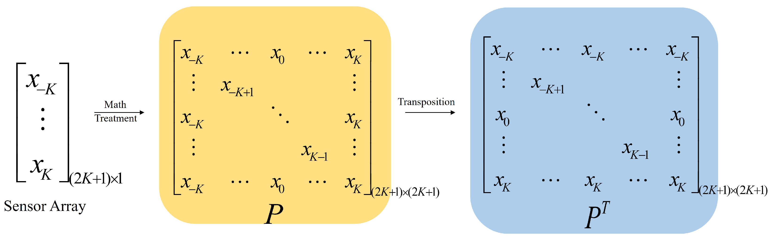
Firstly, consider L narrowband signals of a mixed NF and FF incident onto a spatial sensor array, an SNLA composed of $2K+1$ sensors, and a spacing of d. Using the center of the array as the phase reference point, the sensors in the array can be represented by $x_i$, which belong to a set of integers $\mathbb{P}=\{x_i,i=-K,\dots ,0,\dots ,K\}$.

Assuming there are $L_n$ NF sources and $L-L_n$ FF sources, the output signal of the ith sensor is [26]

$$y_i\left(t\right)=\sum _{l=1}^{L_n}{s}_l\left(t\right)e^{j{\tau }_N}+\sum _{l=L_n+1}^L{s}_l\left(t\right)e^{j{\tau }_F}+n_i\left(t\right)$$

(1)

where $s_l\left(t\right)$ represents the signal of the lth signal source, and ${\tau }_N$ and ${\tau }_F$ represent the propagation delay of the NF source and the FF source to the array, respectively. $n_i\left(t\right)$ represents the noise of the ith sensor. The propagation delay function expression of the NF source is [21,22,43]

$${\tau }_N=-2\pi \frac{d}{\lambda }{x}_{i}sin\left({\theta }_l\right)+\pi \frac{d^2}{\lambda r_l}{x}_i^2{cos}^2\left({\theta }_l\right)$$

(2)

where d represents the sensor spacing and $\lambda$ represents the wavelength of the incident signal. ${\theta }_l$ and $r_l$ represent the direction parameters and the distance parameters of the lth source, respectively. D is set as the physical array aperture and, when the source is located in the Fresnel region, that is, $\begin{array}{c}\hfill 0.62\sqrt{(D^3/\lambda )}<r_l<2D^2/\lambda \end{array}$, in the interval, it is an NF source [44]. Conversely, if the source is in the Fraunhofer region, it is an FF source and its $r_l\to \infty$ propagation delay function is [13,15]

$${\tau }_F=-2\pi \frac{d}{\lambda }{x}_{i}sin{\theta }_l$$

(3)

By simplifying the correlation coefficient in the propagation delay expressions of FF and NF sources, i.e., letting ${\alpha }_l=-2\pi \frac{d}{\lambda }\sin \left({\theta }_l\right)$ and ${\beta }_l=\pi \frac{d^2}{\lambda r_l}{\cos }^2\left({\theta }_l\right)$, we obtain

$${\tau }_N={\alpha }_l{x}_i+{\beta }_l{x}_i^2$$

(4)

$${\tau }_F={\alpha }_l{x}_i$$

(5)

By substituting Equations (4) and (5) into Equation (1), the received signal expression of the receiving sensor is obtained as follows:

$$y_i\left(t\right)=\sum _{l=1}^{L_n}{s}_l\left(t\right)e^{j({\alpha }_i{x}_i+{\beta }_l{x}_i^2)}+\sum _{l=L_n+1}^L{s}_l\left(t\right)e^{j{\alpha }_l{x}_i}+n_i\left(t\right)$$

(6)

The expression of the above equation written into a matrix is as follows:

$$\mathbf{y}\left(t\right)={\mathbf{A}}_N{\mathbf{s}}_N\left(t\right)+{\mathbf{A}}_F{\mathbf{s}}_F\left(t\right)+\mathbf{n}\left(t\right)$$

(7)

where $\mathbf{n}\left(t\right)$ and $\mathbf{y}\left(t\right)$ are the noise and receiving signal vector of size $(2K+1)\times 1$, respectively. ${\mathbf{A}}_N$ and ${\mathbf{A}}_F$ represent the array manifold matrices of the NF and FF sources reaching the $2K+1$ sensors, respectively. In other words, ${\mathbf{A}}_N$ and ${\mathbf{A}}_F$ are matrices of size $(2K+1)\times L_n$ and $(2K+1)\times (L-L_n)$, respectively. ${\mathbf{s}}_N\left(t\right)$ and ${\mathbf{s}}_F\left(t\right)$ represent NF signal source vectors of size $L_n\times 1$ and FF signal source vectors of size $(L-L_n)\times 1$, and there are

$${\left.\mathbf{y}\left(t\right)=\left[\begin{array}{c}{y}_{-K}\left(t\right),...,y_0\left(t\right),...,y_K\left(t\right)\end{array}\right.\right]}^T$$

(8)

$$\mathbf{n}\left(t\right)={\left[n_{-K}\left(t\right),...,n_0\left(t\right),...,n_K\left(t\right)\right]}^T$$

(9)

$${\left.{\mathbf{s}}_N\left(t\right)=\left[\begin{array}{c}{s}_1\left(t\right),...,s_{L_n}\left(t\right)\end{array}\right.\right]}^T$$

(10)

$${\mathbf{s}}_F\left(t\right)={\left[s_{L_n+1}\left(t\right),...,{\mathbf{s}}_L\left(t\right)\right]}^T$$

(11)

$${\mathbf{A}}_N=\left[\mathbf{a}({\theta }_1,r_1),...,\mathbf{a}({\theta }_{L_n},r_{L_n})\right]$$

(12)

$${\mathbf{A}}_F=\left[\mathbf{a}\left({\theta }_{L_n+1}\right),...,\mathbf{a}\left({\theta }_L\right)\right]$$

(13)

where the FF and NF array manifolds are

$$\mathbf{a}({\theta }_L,r_L)={\left[e^{j({\alpha }_L{x}_{-K}+{\beta }_L{x}_{-K}^2)},...,1,...,e^{j({\alpha }_L{x}_K+{\beta }_L{x}_K^2)}\right]}^T$$

(14)

$$\begin{array}{cc}\hfill \mathbf{a}\left({\theta }_L\right)=& \hfill {\left[e^{j{\alpha }_L{x}_{-K}},...,1,...,e^{j{\alpha }_L{x}_K}\right]}^T\hfill \end{array}$$

(15)

In order to better understand the receiving expression, we splice the array manifolds of the FF and NF sources into a global matrix A as follows:

$${\mathbf{A}}_{(2K+1)\times L}=\left[\mathbf{a}({\theta }_1,r_1),...,\mathbf{a}({\theta }_{L_n},r_{L_n}),\mathbf{a}\left({\theta }_{L_n+1}\right),...,\mathbf{a}\left({\theta }_L\right)\right]$$

(16)

Finally, we obtain the signal expression of the receiving sensor as follows:

$${\mathbf{Y}}_{(2K+1)\times 1}={\mathbf{A}}_{(2K+1)\times L}{\mathbf{S}}_{L\times 1}+{\mathbf{N}}_{(2K+1)\times 1}$$

(17)

The above equation divides the signal model of a mixed-field array into two parts—signal propagation and additional noise—where ${\mathbf{S}}_{L\times 1}$ represents the mixed-signal source matrix of size $L\times 1$, ${\mathbf{N}}_{(2K+1)\times 1}$ represents the mixed source noise matrix of size $(2K+1)\times 1$, and ${\mathbf{Y}}_{(2K+1)\times 1}$ represents the received signal matrix of size $(2K+1)\times 1$.

2.2. DCA Signal Model

In this section, we theoretically prove the advantages brought by symmetric arrays and why we need DCA.

This section outlines prior knowledge, namely:

(1)

The source signals are statistically independent, zero-mean random processes with nonzero fourth-order cumulants.

(2)

The sensor noise sequence is zero mean Gaussian white noise and the noise is independent of the signal.

(3)

The sensor array is a symmetric NLA, in which the inter-sensor spacing is within a quarter-wavelength.

Combined with the received signal equation in Section 2.1, the fourth-order cumulant formula of the received signal is as follows:

$$cum\{y_m\left(t\right),y_n^{\ast }\left(t\right),y_p\left(t\right),y_q^{\ast }\left(t\right)\}$$

(18)

where $y_l^{\ast }\left(t\right)$ represents the conjugate form of the received signal. According to Equation (6), we combine and obtain the following:

$$\begin{array}{cc}\hfill & cum\{y_m\left(t\right),y_n^{\ast }\left(t\right),y_p\left(t\right),y_q^{\ast }\left(t\right)\}\hfill \\ \hfill & =\sum _{l=1}^L{c}_{4,s_l}{e}^{j\left[(x_m-x_n+x_p-x_q){\alpha }_l+(x_m^2-x_n^2+x_p^2-x_q^2){\beta }_l\right]}\hfill \end{array}$$

(19)

where the condition satisfied by this equation is $\left.m,n,p,q\in \left[\begin{array}{c}-K,K\end{array}\right.\right]$ and $c_{4,s_l}=\mathrm{cum}\{s_l\left(t\right),s_l^{\ast }\left(t\right),s_l\left(t\right),s_l^{\ast }\left(t\right)\}$. The source signal is a random variable and the corresponding delay propagation is a constant. Equation (18) can be split by using the properties of high-order cumulants.

To mitigate the interference from higher-order cumulants caused by the NF source, we effectively leverage the symmetric properties of the array. We select a symmetric sensor, such as $m=-n,q=-p$; then, in Equation (19), we obtain the expression that $x_m-x_n+x_p-x_q\ne 0,x_m^2-x_n^2+x_p^2-x_q^2=0$. The high-order cumulant formula is as follows:

$$\begin{array}{cc}\hfill & cum\{y_m\left(t\right),y_n^{\ast }\left(t\right),y_p\left(t\right),y_q^{\ast }\left(t\right)\}\hfill \\ \hfill & =\sum _{l=1}^L{c}_{4,{\mathrm{s}}_l}{e}^{j2(x_m-x_p){\alpha }_l}\hfill \end{array}$$

(20)

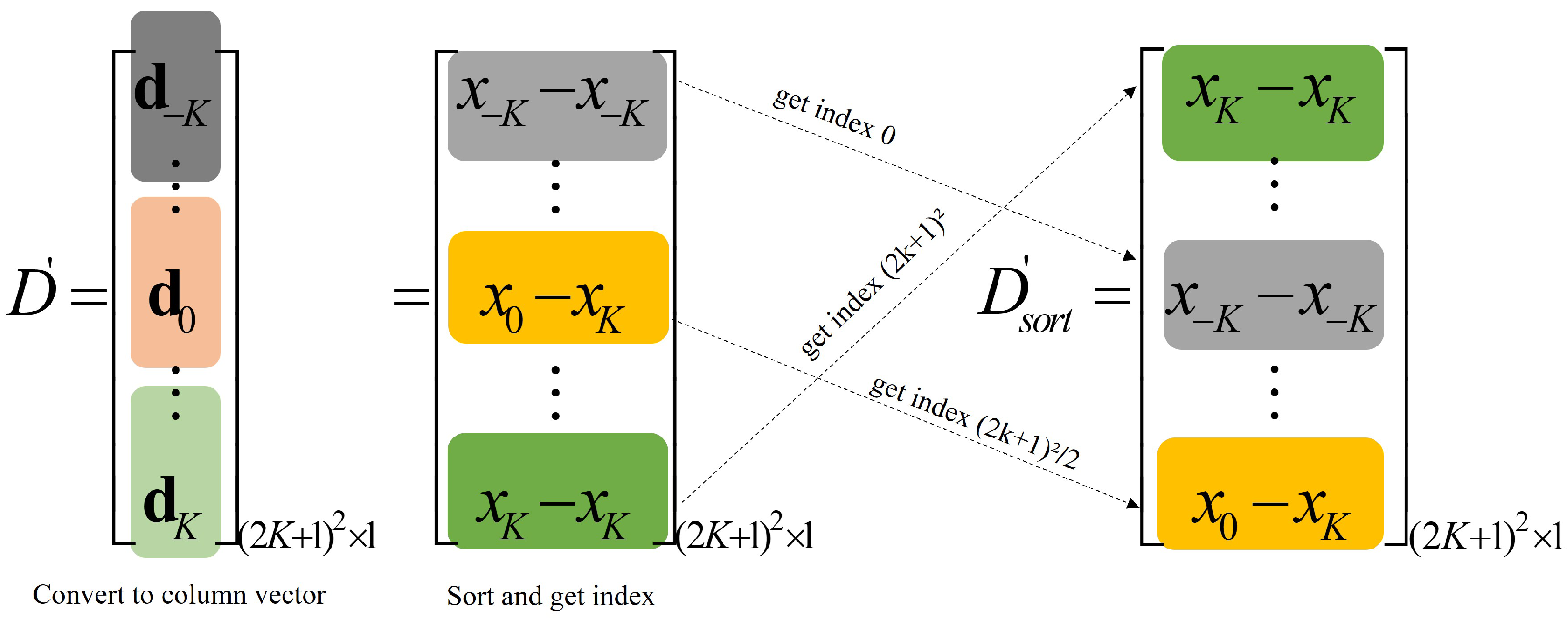
By matrixizing the previous equation, we obtain:

$$\mathbf{F}=\mathbf{E}{\mathbf{C}}_{4.s_l}{\mathbf{E}}^H=\sum _{l=1}^L{c}_{4,s_l}\mathbf{e}\left({\theta }_l\right){\mathbf{e}}^H\left({\theta }_l\right)$$

(21)

where ${\mathbf{C}}_{4.s_l}=diag(c_{4,s_1},c_{4,s_2},...,c_{4,s_l})$, $\mathbf{F}$ is a cumulant matrix, and $\mathbf{E}=\left[\begin{array}{c}\mathbf{e}\left({\theta }_1\right),\mathbf{e}\left({\theta }_2\right),...,\mathbf{e}\left({\theta }_l\right)\end{array}\right]$, where $\mathbf{e}\left({\theta }_l\right)={\left[e^{j2{\alpha }_l{x}_{-K}},e^{j2{\alpha }_l{x}_{-K+1}},...,1,...,e^{j2{\alpha }_l{x}_{K-1}},e^{j2{\alpha }_l{x}_K}\right]}^T$. We vectorize $\mathbf{F}$ to obtain

$$z=vec\left(\mathbf{F}\right)={\mathbf{E}}_c\mathbf{c}$$

(22)

where $\mathbf{c}={\left[c_{4,x_1},c_{4,x_2},...,c_{4,x_l}\right]}^T$ and ${\mathbf{E}}_c$ denotes the matrix after Kronecker multiplication of the original matrix. ${\mathbf{E}}_c=[{\mathbf{e}}_c\left({\theta }_1\right),{\mathbf{e}}_c\left({\theta }_2\right),...,{\mathbf{e}}_c\left({\theta }_l\right)]$, where ${\mathbf{e}}_c\left({\theta }_l\right)={\mathbf{e}}^{\ast }\left({\theta }_l\right)\otimes \mathbf{e}\left({\theta }_l\right)$. Matrix ${\mathbf{E}}_c$ is equivalent to the manifold matrix of set $\mathrm{P}$, where $\mathrm{P}=\{x_p-x_q,p,q=-K,...,0,...,K\}$. We call a set such as set $\mathrm{P}$ a DCA.

2.3. The Technology of Source Localization

According to the previous section, we need to apply a symmetrical array to eliminate the high-order cumulants caused by NF sources and require a DCA to perform related algorithm analysis. In particular, we need to apply an SNLA to perform DOA and range assessments. Based on the consecutive lags in the virtual array of SNLAs, we apply the array model theory and the spatial smoothing method [42,45] to construct the correlation matrix and apply the MUSIC algorithm [46] to distinguish the DOA of the signal source.

Firstly, we obtain the covariance matrix ${\mathbf{R}}_{xx}$ of the received signal according to the received signal matrix $\mathbf{X}\left(t\right)$, where ${\mathbf{R}}_{xx}=E\left\{\mathbf{X}\left(t\right){\mathbf{X}}^H\left(t\right)\right\}$. Afterward, we use the longest continuous subarray in the DCA, which is equivalent to a continuous ULA, to apply the spatial smoothing algorithm. Let the longest consecutive lags of the DCA be $\mathrm{U}=[-H_m,H_m]$. By using the difference index of the elements generated in the difference operation and the covariance matrix ${\mathbf{R}}_{xx}$ of the received signal, the smooth value of each index of each element in $\mathrm{U}=[-H_m,H_m]$ is obtained (the concept of the index can be explained via the difference index in Appendix A) and the corresponding construction vector is obtained:

$$\mathbf{z}={\mathbf{E}}_{ss}\mathbf{c}$$

(23)

where ${\mathbf{E}}_{ss}$ is a $(2H_m+1)\times l$ manifold matrix of a continuous array element U. The vector $\mathbf{z}$ has $(2H_m+1)$ elements. Using vector $\mathbf{z}$ to construct a spatial smoothing matrix [42], we obtain the following:

$${\mathbf{R}}_{ss}\triangleq \frac{1}{H_m+1}\sum _{l=1}^{H_m+1}{\mathbf{z}}_l{\mathbf{z}}_l^H$$

(24)

where ${\mathbf{z}}_l$ denotes the subvector corresponding to the $H_m+1-l$th row to the $2H_m+2-l$th row in the vector $\mathbf{z}$. Then, we perform eigenvalue decomposition on ${\mathbf{R}}_{ss}$ and we obtain the following:

$${\mathbf{R}}_{ss}={\mathbf{U}}_s{\Sigma }_s{\mathbf{U}}_s^{\mathrm{H}}+{\mathbf{U}}_{\mathrm{N}}{\Sigma }_{\mathrm{N}}{\mathbf{U}}_{\mathrm{N}}^{\mathrm{H}}$$

(25)

where ${\mathbf{U}}_{\mathbf{s}}$ is the subspace spanned by the feature vector corresponding to the large eigenvalue, that is, the signal subspace. Furthermore, ${\mathbf{U}}_{\mathbf{N}}$ is the subspace spanned by the feature vector corresponding to the small eigenvalue, that is, the noise subspace. Using the orthogonal relationship between the steering vector in the signal subspace and the noise subspace, we can write the 1D spectral peak search function:

$$f\left(\theta \right)={\left[{\mathbf{a}}^{\mathrm{H}}\left(\theta \right){\mathbf{U}}_{\mathrm{N}}{\mathbf{U}}_{\mathrm{N}}^{\mathrm{H}}\mathbf{a}\left(\theta \right)\right]}^{-1}$$

(26)

In the one-dimensional MUSIC spectrum, there are L distinct peaks, with each corresponding to the arrival angles of L different sources. These angles of arrival are denoted as ${\theta }_i=\{{\theta }_1,\dots ,{\theta }_{L_n},{\theta }_{L_{n+1}}\dots ,{\theta }_L\}$. Here, ${\theta }_N=\{{\theta }_1,\dots ,{\theta }_{L_n}\}$ specifically represents the angles of arrival for NF sources. However, in practical scenarios, the angular difference between FF and NF sources remains uncertain. To address this, we utilize the orthogonal relationship between the steering vector in the signal subspace and the noise subspace, enabling us to delineate the spectral peak in a two-dimensional framework:

$$f(\theta ,r)={\left[{\mathbf{a}}^{\mathbf{H}}(\theta ,r){\mathbf{U}}_{\mathbf{N}}{\mathbf{U}}_{\mathbf{N}}^{\mathbf{H}}\mathbf{a}(\theta ,r)\right]}^{-1}$$

(27)

After conducting a one-dimensional MUSIC spectral peak search using Equation (26), the obtained arrival angles are ${\theta }_i=\{{\theta }_1,...,{\theta }_{L_n},{\theta }_{L_{n+1}}...,{\theta }_L\}$. Subsequently, inserting these identified arrival angles into Equation (27) yields the desired result:

$$p({\theta }_i,r)={\left[{\mathbf{a}}^{\mathbf{H}}({\theta }_i,r){\mathbf{U}}_{\mathbf{N}}{\mathbf{U}}_{\mathbf{N}}^{\mathbf{H}}\mathbf{a}({\theta }_i,r)\right]}^{-1}$$

(28)

At this time, the spectral peak search is performed on the distance r and the corresponding result of the search is [45] as follows:

$$r_m=\underset{r}{min}{\left[{\mathbf{a}}^{\mathbf{H}}({\theta }_i,r){\mathbf{U}}_{\mathbf{N}}{\mathbf{U}}_{\mathbf{N}}^{\mathbf{H}}\mathbf{a}({\theta }_i,r)\right]}^{-1}$$

(29)

If the search result is located in the NF region, then the i-th angle corresponds to the NF source; if it is located in the FF region, it is an FF source.

3. Array Configuration

3.1. Array Structure

In this section, we introduce an SNLA configuration, named a symmetric double-supplemented nested array, designed for mixed source localization in both NF and FF scenarios. The SDSNA configuration exhibits several outstanding characteristics. Firstly, both its array configuration and maximum consecutive lags can be written as expressions. Additionally, it surpasses other SNLAs in terms of its longer consecutive lags and a more expansive physical array aperture. These features collectively enhance its performance in source localization tasks.

The configuration of SDSNA is shown in Figure 1, which consists of seven parts, including three ULAs and four symmetrical supplemented sensors. ULA1 has N sensors with an interval of d, where d is the spacing between sensors. ULA2 and ULA3 are ULAs with $(N+1)d$ internal sensor spacing and $(N+1)d$ spacing from ULA1. Supplement 1, as an independent supplemented sensor, can effectively fill in the holes generated by the DCA of ULA1 and ULA2. It is separated from ULA2 and ULA3 by $Nd$. As another independent supplemented sensor, Supplement 2 is $(N+1)d$ away from Supplement 1 and its function is to effectively expand the physical aperture of the array, introducing greater space for improvement in the DOF. For SDSNA, we assume that $M>3$, $N>3$, $Q=N+2M+4>13$.

The sensors position of SDSNA can be expressed as $\mathbb{R}={\mathbb{R}}_1\cup {\mathbb{R}}_2\cup {\mathbb{R}}_3\cup {\mathbb{R}}_4\cup {\mathbb{R}}_5\cup {\mathbb{R}}_6\cup {\mathbb{R}}_7$, where ${\mathbb{R}}_1$ is the central ULA array; ${\mathbb{R}}_2$ and ${\mathbb{R}}_3$ are ULA2 and ULA3, respectively; ${\mathbb{R}}_4$ and ${\mathbb{R}}_5$ represent the right and left parts of Supplement 1, respectively; and ${\mathbb{R}}_6$ and ${\mathbb{R}}_7$ represent the right and left parts of Supplement 2, respectively. The SDSNA configuration is described as follows:

$${\mathbb{R}}_1=\left\{R_{m_1}\right|R_{m_1}=m_1-(N-1)/2\}$$

(30)

$${\mathbb{R}}_2=\{R_{m_2}\left|R_{m_2}\right.=(3N+1)/2+(N+1)m_2\}$$

(31)

$${\mathbb{R}}_3=\left\{R_{m_3}\right|R_{m_3}=-(3N+1)/2-(N+1)m_3\}$$

(32)

$${\mathbb{R}}_4=\{R_{m_4}\left|R_{m_4}\right.=(N+1)M+(N-3)/2\}$$

(33)

$${\mathbb{R}}_5=\{R_{m_5}\left|R_{m_5}\right.=-(N+1)M-(N-3)/2\}$$

(34)

$${\mathbb{R}}_6=\{R_{m_6}\left|R_{m_6}\right.=(N+1)(M+1)+(N-3)/2\}$$

(35)

$${\mathbb{R}}_7=\{R_{m_7}\left|R_{m_7}\right.=-(N+1)(M+1)-(N-3)/2\}$$

(36)

where $m_1\in [0,N-1]$, $m_2,m_3\in [0,M-2]$.

For the SDSNA configuration, the DCA is $\mathbb{S}={\mathbb{S}}_s\cup {\mathbb{S}}_c$, where ${\mathbb{S}}_s$ is a self-differential set and ${\mathbb{S}}_c$ is a cross-differential set. Simultaneously, the DCA can be divided into two components: $\mathbb{S}={\mathbb{S}}^{+}\cup {\mathbb{S}}^{-}$. Due to the symmetric structure of the array, theoretical derivations only focus on the positive half-axis of the DCA. For the DCA component ${\mathbb{S}}^{+}$, the relationship can be expressed as follows: ${\mathbb{S}}^{+}={\mathbb{S}}_s^{+}\cup {\mathbb{S}}_c^{+}$. Then, ${\mathbb{S}}_s^{+}$ is

$${\mathbb{S}}_s^{+}={\mathbb{S}}_{11}\cup {\mathbb{S}}_{22}\cup {\mathbb{S}}_{33}$$

(37)

where

$$\begin{array}{cc}\hfill & {\mathbb{S}}_{11}=\left\{s_{11}\right|s_{11}=m_1\},\hfill \\ \hfill & {\mathbb{S}}_{22}=\left\{s_{22}\left|s_{22}=(N+1)m_2\right\},\right.\hfill \\ \hfill & {\mathbb{S}}_{33}=\left\{s_{33}\left|s_{33}\right.=(N+1)m_3\right\},\hfill \end{array}$$

(38)

where $m_1\in [0,N-1]$, $m_2,m_3\in [0,M-2]$. Since ${\mathbb{R}}_4$, ${\mathbb{R}}_5$, ${\mathbb{R}}_6$, and ${\mathbb{R}}_7$ are independent single sensors, their self-differential set is zero, i.e., ${\mathbb{S}}_{44}$, ${\mathbb{S}}_{55}$, ${\mathbb{S}}_{66}$, and ${\mathbb{S}}_{77}$ are all zero. The set of ${\mathbb{S}}_c^{+}$ is as follows:

$$\begin{array}{cc}\hfill {\mathbb{S}}_c^{+}& =({\mathbb{S}}_{13}\cup {\mathbb{S}}_{21})\cup ({\mathbb{S}}_{15}\cup {\mathbb{S}}_{41})\cup ({\mathbb{S}}_{61}\cup {\mathbb{S}}_{17})\cup ({\mathbb{S}}_{42}\cup {\mathbb{S}}_{35})\hfill \\ \hfill & \cup ({\mathbb{S}}_{62}\cup {\mathbb{S}}_{37})\cup ({\mathbb{S}}_{43}\cup {\mathbb{S}}_{25})\cup ({\mathbb{S}}_{63}\cup {\mathbb{S}}_{27})\hfill \\ \hfill & \cup ({\mathbb{S}}_{64}\cup {\mathbb{S}}_{57})\cup ({\mathbb{S}}_{65}\cup {\mathbb{S}}_{47})\cup {\mathbb{S}}_{23}\cup {\mathbb{S}}_{45}\cup {\mathbb{S}}_{67}\hfill \end{array}$$

(39)

where

$${\mathbb{S}}_{13}=\left\{s_{13}\right|s_{13}=N+1+(N+1)m_3+m_1\}$$

(40)

$${\mathbb{S}}_{21}=\left\{s_{21}\right|s_{21}=2N+(N+1)m_2-m_1\}$$

(41)

$${\mathbb{S}}_{15}=\left\{s_{15}\right|s_{15}=(N+1)M+m_1-1\}$$

(42)

$${\mathbb{S}}_{41}=\left\{s_{41}\right|s_{41}=(N+1)M-m_1+N-2\}$$

(43)

$${\mathbb{S}}_{61}=\left\{s_{61}\right|s_{61}=(N+1)(M+1)-m_1+N-2\}$$

(44)

$${\mathbb{S}}_{17}=\left\{s_{17}\right|s_{17}=(N+1)(M+1)-m_1-1\}$$

(45)

$${\mathbb{S}}_{35}=\left\{s_{35}\right|s_{35}=(N+1)(M-m_3)-N-2\}$$

(46)

$${\mathbb{S}}_{42}=\left\{s_{42}\right|s_{42}=(N+1)(M-m_2)-N-2\}$$

(47)

$${\mathbb{S}}_{37}=\left\{s_{37}\right|s_{37}=(N+1)(M+1-m_3)-N-2\}$$

(48)

$${\mathbb{S}}_{62}=\left\{s_{62}\right|s_{62}=(N+1)(M+1-m_2)-N-2\}$$

(49)

$${\mathbb{S}}_{25}=\left\{s_{25}\right|s_{25}=(N+1)(M+m_2)+2N-1\}$$

(50)

$${\mathbb{S}}_{43}=\left\{s_{43}\right|s_{43}=(N+1)(M+m_3)+2N-1\}$$

(51)

$${\mathbb{S}}_{27}=\left\{s_{27}\right|s_{27}=(N+1)(M+1+m_2)+2N-1\}$$

(52)

$${\mathbb{S}}_{63}=\left\{s_{63}\right|s_{63}=(N+1)(M+1+m_3)+2N-1\}$$

(53)

$${\mathbb{S}}_{23}=\left\{s_{23}\right|s_{23}=(N+1)({\mathfrak{m}}_2+m_3)+3N+1\}$$

(54)

$${\mathbb{S}}_{45}=\left\{s_{45}\right|s_{45}=2(N+1)M+N-3\}$$

(55)

$${\mathbb{S}}_{67}=\left\{s_{67}\right|s_{67}=2(N+1)(M+1)+N-3\}$$

(56)

$${\mathbb{S}}_{64}=\left\{s_{64}\right|s_{64}=N+1\}$$

(57)

$${\mathbb{S}}_{57}=\left\{s_{57}\right|s_{57}=N+1\}$$

(58)

$${\mathbb{S}}_{65}=\left\{s_{65}\right|s_{65}=(N+1)(2M+1)+N-3\}$$

(59)

$${\mathbb{S}}_{47}=\left\{s_{47}\right|s_{47}=(N+1)(2M+1)+N-3\}$$

(60)

where $m_1\in [0,N-1]$, $m_2,m_3\in [0,M-2]$.

3.2. Array Propositions and Deductions

We present the DCA properties of the SDSNA in the following sections.

3.2.1. Array Symmetry Propositions and Deductions

Proposition 1.

Due to the symmetry of the SDSNA, the DCAs of SDSNA are

$$\begin{array}{c}{\mathbb{S}}_{13}={\mathbb{S}}_{21},{\mathbb{S}}_{41}={\mathbb{S}}_{15},{\mathbb{S}}_{61}={\mathbb{S}}_{17},\\ {\mathbb{S}}_{42}={\mathbb{S}}_{35},{\mathbb{S}}_{62}={\mathbb{S}}_{37},{\mathbb{S}}_{43}={\mathbb{S}}_{25},\\ {\mathbb{S}}_{63}={\mathbb{S}}_{27},{\mathbb{S}}_{64}={\mathbb{S}}_{57},{\mathbb{S}}_{65}={\mathbb{S}}_{47}.\end{array}$$

(61)

Proof of Proposition 1.

According to the set expression Equation (43), the expression of element $s_{41}$ in set ${\mathbb{S}}_{41}$ is $\begin{array}{c}\hfill s_{41}=(N+1)M-m_1+N+2\end{array}$, where $m_1\in [0,N-1]$, $m_2,m_3\in [0,M-2]$. Let $m_1^{\prime }=-m_1+N-1,m_1^{\prime }\in [0,N-1]$; then, $s_{41}$ can be expressed as follows:

$$s_{41}=(N+1)M+m_1^{\prime }-1$$

(62)

By comparing the set expression Equation (62) and the set expression Equation (42), we obtain $s_{41}\in {\mathbb{S}}_{15}$.

According to the set expression Equation (42), the expression of element $s_{15}$ in set ${\mathbb{S}}_{15}$ is $s_{15}=(N+1)M+m_1-1$, where $m_1\in [0,N-1]$, $m_2,m_3\in [0,M-2]$. Let $m_1^{\prime }=-m_1+N-1,m_1^{\prime }\in [0,N-1]$; then,

$$s_{15}=(N+1)M+m_1^{\prime }+N-2$$

(63)

By comparing the set expression Equation (63) and the set expression Equation (43), we obtain $s_{15}\in {\mathbb{S}}_{41}$.

In summary, we obtain ${\mathbb{S}}_{15}={\mathbb{S}}_{41}$. Similarly, we can prove other equations in Equation (61). Therefore, the proof is complete. □

In this way, ${\mathbb{S}}^{+}$ and ${\mathbb{S}}_c^{+}$ can be expressed as follows:

$$\begin{array}{cc}\hfill {\mathbb{S}}_c^{+}& \hfill ={\mathbb{S}}_{21}\cup {\mathbb{S}}_{41}\cup {\mathbb{S}}_{61}\cup {\mathbb{S}}_{42}\cup {\mathbb{S}}_{62}\cup {\mathbb{S}}_{43}\hfill \\ & \hfill \cup {\mathbb{S}}_{63}\cup {\mathbb{S}}_{23}\cup {\mathbb{S}}_{45}\cup {\mathbb{S}}_{67}\cup {\mathbb{S}}_{64}\cup {\mathbb{S}}_{65}\hfill \end{array}$$

(64)

$${\mathbb{S}}^{+}={\mathbb{S}}_c^{+}\cup {\mathbb{S}}_{11}\cup {\mathbb{S}}_{22}$$

(65)

3.2.2. The Longest Continuous Lag Propositions and Deductions

Proposition 2.

In the SDSNA, the DCA set $\mathbb{S}$ has the longest continuous lags $[-MN-M-2N, MN+M+2N]$ and the maximum continuous length is $2MN+2M+4N+1$, which is the DOF of the SDSNA.

Proof of Proposition 2.

Setting ${\mathbb{S}}_a={\mathbb{S}}_{11}\cup {\mathbb{S}}_{21}\cup {\mathbb{S}}_{35}$, we first prove that the longest consecutive element in ${\mathbb{S}}_a$ is $[0,(N+1)M+2N-1]$.

According to the set expression Equation (41), ${\mathbb{S}}_{21}=\left\{s_{21}\right|s_{21}=2N+(N+1)m_2-m_1$}. Let $m_1^{\prime }=-m_1+N-1,m_2^{\prime }=m_2+1$; then, we obtain

$${\mathbb{S}}_{21}=(N+1)m_2^{\prime }+m_1^{\prime }$$

(66)

where $m_1^{\prime }\in [0,N-1],m_2^{\prime }\in [1,M-1]$. By comparing with the set expression Equation (38), we obtain $s_{11}=m_1$, where $m_1\in [0,N-1]$; the following can be obtained:

$$s_{11}\cup s_{21}=(N+1)m_{a1}^{\prime }+m_1$$

(67)

where $\begin{array}{c}\hfill m_{a1}^{\prime }\in [0,M-1],m_1\in [0,N-1]\end{array}$. Therefore, the integer elements of ${\mathbb{S}}_{11}\cup {\mathbb{S}}_{21}$ are consecutive in the ranges $\left[\begin{array}{c}0,(N-1)\end{array}\right],\left[\begin{array}{c}N+1,2N\end{array}\right],...,\left[\begin{array}{c}(N+1)M,(N+1)M+N-1\end{array}\right]$. We can observe that there are holes between the intervals expressed by

$$s_h=(N+1)m_h+N$$

(68)

where $m_h\in [0,M-2]$. According to the set expression Equation (46), we obtain that $s_{35}$ in ${\mathbb{S}}_{35}$ is $s_{35}=\{s_{35}\left|s_{35}(N+1)(M-m_3)-N-2\right\}$, $m_3\in [0,M-2]$. By setting $m_3^{\prime }=M-2-m_3$, we obtain

$$s_{35}=(N+1)m_3^{\prime }+N,m_3^{\prime }\in [0,M-2]$$

(69)

Compared with the set expression Equation (68), we can obtain ${\mathbb{S}}_{35}={\mathbb{S}}_h$; thus, it can be identified that the set expression Equation (69) just fills the hole. We obtain that $S_a$ are consecutive in $[0,(N+1\left)\right(M-1)+N-1]$. Furthermore, the set expression of ${\mathbb{S}}_a$ is as follows:

$$s_a=m_a,m_a\in \left[\begin{array}{c}0,(N+1)(M-1)+N-1\end{array}\right]$$

(70)

Then, we set ${\mathbb{S}}_b={\mathbb{S}}_a\cup {\mathbb{S}}_{41}$. According to set expression Equation (43), we obtain $s_{41}=\left\{s_{41}\right|s_{41}=(N+1)M-m_1+N-2\}$. Let $m_4^{\prime }=N-m_1,m_4^{\prime }\in [1,N]$, $s_{41}$ become

$$s_{41}=(N+1)(M-1)+N-1+m_4^{\prime }$$

(71)

Compared to the set expression Equation (70), we obtain

$$s_b=m_b,m_b\in \left[0,(N+1)(M-1)+2N-1\right]$$

(72)

Then, we set ${\mathbb{S}}_c={\mathbb{S}}_b\cup {\mathbb{S}}_{23}$ and, from the set expression Equation (54), we obtain $s_{23}=\left\{s_{23}\right|s_{23}=(N+1)({\mathfrak{m}}_2+m_3)+3N+1\}$, $m_2,m_3\in [0,M-2]$. Let $m_5^{\prime }=m_2+m_3+1$, $m_5^{\prime }\in [1,2M-3]$. Then, we obtain

$$s_{23}=(N+1)m_5^{\prime }+2N,m_5^{\prime }\in [1,2M-3]$$

(73)

when $m_s^{\prime }=M-1,s_{23}=(N+1)(M-1)+2N$. Then, compared to the set expression Equation (72), we know that ${\mathbb{S}}_c$ are consecutive in $\left[0,(N+1)(M-1)+2N\right]$ and the expression of ${\mathbb{S}}_c$ is as follows:

$${\mathbb{S}}_c=\left\{m_{c_1}\right\}\cup \{(N+1)m_{c_2}+2N\}$$

(74)

where $m_{c_1}\in [0,(N+1)(M-1)+2N],m_{c_1}\in [M,2M-3]$. Then, we set ${\mathbb{S}}_d={\mathbb{S}}_c\cup {\mathbb{S}}_{25}$, forming the set expression Equation (50), and we obtain ${\mathbb{S}}_{25}=\left\{s_{25}\right|s_{25}=(N+1)(M+m_2)+2N-1\},m_2\in [0,M-2]$. Setting $m_6^{\prime }=M-m_2-1,m_6^{\prime }\in \left[M-1,2M-3\right]$, we obtain

$$s_{25}=(N+1)m_6^{\prime }+3N$$

(75)

where $m_6^{\prime }\in [M-1,2M-3]$; then, we obtain

$${\mathbb{S}}_d=\left\{m_{d_1}\right\}\cup \{(N+1)m_{d_2}+n_d\}\cup \{2(N+1)M-3\}$$

(76)

where $m_{d_1}\in \left[0,(N+1)(M-1)+2N\right],m_{d_2}\in \left[M-1,2M-4\right]$, ${\mathfrak{n}}_d\in \left[\begin{array}{c}3N,3N+1\end{array}\right]$. According to the set expression Equation (38), we obtain ${\mathbb{S}}_{22}=\left\{s_{22}\right|s_{22}=(N+1)m_2\},m_2\in [0,M-2]$ and we can know that $0\le s_{22}\le (N+1)(M-2)$. In other words, $s_{22}\in {\mathbb{S}}_a$. Similarly, $S_{41}$ also exhibits the condition that $S_{41}\in {\mathbb{S}}_a$. According to Equations (55), (56), and (59), we obtain that ${\mathbb{S}}_{45}$, ${\mathbb{S}}_{67}$, and ${\mathbb{S}}_{65}$ only contain one element, which is not consecutive with others. Thus, we obtain ${\mathbb{S}}_e={\mathbb{S}}_d\cup {\mathbb{S}}_{45}\cup {\mathbb{S}}_{67}\cup {\mathbb{S}}_{65}$, the closed form of which expression is as follows:

$$\begin{array}{cc}\hfill {\mathbb{S}}_e& =\left\{m_{e_1}\right\}\cup \{(N+1)m_{e_2}+n_e\}\cup \{2(N+1)(M+1)+N-3\}\hfill \\ \hfill & \cup \left\{2\right(N+1)M-3\}\cup \left\{\right(N+1\left)\right(2M+1)+N-3\}\hfill \\ \hfill & \cup \left\{2\right(N+1)M+N-3\}\hfill \end{array}$$

(77)

where $m_{e_1}\in \left[0,(N+1)(M-1)+2N\right],m_{e_2}\in \left[M-1,2M-4\right]$, ${\mathfrak{n}}_e\in \left[\begin{array}{c}3N,3N+1\end{array}\right]$. We set ${\mathbb{S}}_f={\mathbb{S}}_e\cup {\mathbb{S}}_{61}$ and, using Equation (44), the expression of $s_{61}$ is ${\mathbb{S}}_{61}=\left\{s_{61}\right|s_{61}=(N+1)(M+1)-m_1+N-2\},m_1\in [0,N-1]$. After making some mathematical changes, we obtain

$$s_{61}=(N+1)(M-1)+2N-m_1$$

(78)

Let $m_7^{\prime }=N-m_1,m_7^{\prime }\in [1,N]$; then, we obtain

$$s_{61}=(N+1)(M-1)+2N+m_7^{\prime }$$

(79)

Comparing Equation (79) with Equation (77), ${\mathbb{S}}_e$ has a consecutive length, which is $(N+1)(M-1)+2N$. On the basis of $(N+1)(M-1)+2N$, ${\mathbb{S}}_{61}$ increases the length of another $m_7^{\prime }$. Thus, we obtain that ${\mathbb{S}}_f$ are consecutive in $[0,(N+1\left)\right(M-1)+3N]$. On the basis of (73), we obtain $s_{23}=(N+1)m_5^{\prime }+3N+1$ when $m_5^{\prime }=M-1$. Thus, ${\mathbb{S}}_f$ are consecutive in $[0,(N+1\left)\right(M-1)+1+3N]$ and the expression of ${\mathbb{S}}_f$ is as follows:

$$\begin{array}{cc}\hfill {\mathbb{S}}_f& =\left\{m_{f_1}\right\}\cup \{2(N+1)(M+1)+N-3\}\hfill \\ \hfill & \cup \left\{2\right(N+1)M-3\}\cup \left\{\right(N+1\left)\right(2M+1)+N-3\}\hfill \\ \hfill & \cup \left\{2\right(N+1)M+N-3\}\hfill \end{array}$$

(80)

where $m_{f_1}\in [0,(N+1)(M-1)+3N+1]$. According to the set expression Equation (49), ${\mathbb{S}}_{62}=\left\{s_{62}\right|s_{62}=(N+1)(M+1-m_2)-N-2\}$, where $m_2\in [0,M-2]$. After performing some mathematical changes, we obtain

$$s_{62}=(N+1)(M-1)+N-(N+1)m_2$$

(81)

We can see that $0\le s_{62}\le (N+1)(M-1)+3N+1$; thus, ${\mathbb{S}}_{62}$ is covered by the consecutive part of ${\mathbb{S}}_f$. We set ${\mathbb{S}}^{+}={\mathbb{S}}_f\cup {\mathbb{S}}_{63}$ and $s_{63}$ in ${\mathbb{S}}_{63}$, which is $s_{63}=(N+1)(M+1+m_3)+2N-1$, $m_3\in [0,M-1]$. When we set $m_3=M-2$, we obtain $s_{63}=2(N+1)M+N-2$. Compared to Equation (80), we can obtain the final expression of consecutive lags as follows:

$$\begin{array}{cc}\hfill & {\mathbb{S}}^{+}=\left\{m_f\right\}\cup \{2(N+1)(M+1)+n_f\}\hfill \\ \hfill & \cup \left\{2\right(N+1)M-3\}\cup \left\{\right(N+1\left)\right(2M+1)+N-3\}\hfill \\ \hfill & \cup \left\{2\right(N+1)M+N-3\}\hfill \end{array}$$

(82)

where $m_{f_1}\in [0,(N+1)(M-1)+3N+1],n_f\in [N-3,N-2]$.

Therefore, the maximum number of consecutive lags of ${\mathbb{S}}^{+}$ is in the range of $[0,(N+1\left)\right(M-1)+3N+1]$. Since ${\mathbb{S}}^{+}$ is symmetric with ${\mathbb{S}}^{-}$, $\mathbb{S}$ has the longest consecutive lags in the range of $[-(N+1\left)\right(M-1)-3N-1,(N+1\left)\right(M-1)+3N+1]$, and the number of lags is $2MN+2M+4N+1$, thus completing the proof. In order to obtain the longest consecutive lags, we provide the optimal configuration of M and N in the array. □

3.2.3. Array Optimal Configuration Propositions and Deductions

Proposition 3.

When $N=round\left(\frac{Q+1}{2}\right)$ and $M=\frac{1}{2}\left(Q-round\left(\frac{Q+1}{2}\right)-2\right)$, the maximum number of consecutive lags can be achieved.

Proof of Proposition 3.

We know the consecutive lags in the DCA based on the previous discussion. The key to maximizing these consecutive lags lies within optimizing the quantities of sub-nested arrays, denoted as M and N. The formula for the total number of array sensors is given by $Q=N+2(M-1)+4$. By simplifying this expression, we obtain $Q=N+2+2M$. Therefore, we can express M as follows:

$$\begin{array}{c}\hfill M=\frac{1}{2}\left(Q-N-2\right)\end{array}$$

(83)

By substituting Equation (83) into the maximum number of consecutive lags, we obtain the following:

$$\begin{array}{cc}\hfill L& =2MN+2M+4N+1\hfill \\ & =2\times \frac{1}{2}\left(Q-N-2\right)N+2\times \frac{1}{2}\left(Q-N-2\right)+4N+1\hfill \\ & =-N^2+(Q+1)N+Q-1\hfill \end{array}$$

(84)

We can obtain the maximum value of the quadratic function by deriving the quadratic concave function L.

Then, there is a maximum value when $N=round\left(\frac{Q+1}{2}\right)$, which also means that it is the best configuration for the array. Here, $M=\frac{1}{2}(Q-N-2)=\frac{1}{2}\left(Q-round\left(\frac{Q+1}{2}\right)-2\right)$, where round() is a rounding operation. This completes the proof. □

Based on the above calculation results, we discuss the four cases of the number of sensors Q and we provide the optimal array configuration of the sensor in

Table 1. Optimum array configuration for SDSNA.

Q	Optimal M, N	Number of Consecutive Lags
4k	$M=\frac{Q-4}{4},N=\frac{Q}{2}$	$\frac{Q^2+6Q-4}{4}$
4k + 1	$M=\frac{Q-5}{2},N=\frac{Q+1}{2}$	$\frac{Q^2+6Q-3}{4}$
4k + 2	$M=\frac{Q-6}{2},N=\frac{Q+2}{2}$	$\frac{Q^2+6Q-4}{4}$
4k + 3	$M=\frac{Q-3}{2},N=\frac{Q-1}{2}$	$\frac{Q^2+6Q-7}{4}$

.

4. Numerical Experiment

In this section, five arrays, namely, ISNA [38], SDNA [39], SDCA [40], CSNA [37], and SFNA [47], were used for the comparison experiments, where the SFNA was used for the coupling part of the comparison due to its better coupling properties.

The numerical experiment is divided into three main parts:

• The DOF and aperture sizes of the ISNA, SDNA, SDCA, CSNA, and SDSNA are compared under varying numbers of sensors.
• Both the coupling matrix amplitude diagrams of the ISNA, SDNA, SDCA, CSNA, SFNA, and SDSNA under a limited number of sensors and the specific values of coupling leakage under different numbers of sensors are compared.
• The performance errors of the ISNA, SDNA, SDCA, CSNA, and SDSNA for mixed-field sources under different experimental conditions are compared.

The numerical experiments were carried out from two perspectives, firstly, 1.2 experiments were carried out for the physical properties of the arrays to compare the arrays’ intrinsic properties and, thus, measure the array performance. Subsequently, the DOA correlation algorithm was applied to the arrays, and DOA and range were resolved under different experimental conditions to compare the estimation errors between the arrays.

To ensure the reliability of the DOF experimental comparisons, we provided four optimal array configurations for comparing SNLAs (

Table 2. Optimum array configurations for four symmetric non-uniform linear arrays (SNLAs).

Name	Q	Optimal M, N	Number of Consecutive Lags
ISNA	4K + 1	$M=\frac{Q-1}{4}, N=\frac{Q+3}{4}$ *	$\frac{Q^2+4Q-1}{4}$ *
	4K + 3	$M=\frac{Q-3}{4}, N=\frac{Q+5}{4}$ *	$\frac{Q^2+4Q-1}{4}$ *
SDNA	4K + 1	$M=\frac{Q+3}{4}, N=\frac{Q-1}{4}$	$\frac{Q^2+10Q-3}{8}$ *
	4K + 3	$M=\frac{Q+1}{4}, N=\frac{Q+1}{4}$	$\frac{Q^2+10Q+1}{8}$ *
SDCA	4K	$M=\frac{Q}{4}, N=\frac{Q}{4}$	$\frac{Q^2+4Q+15}{4}$
	4K + 1	$M=\frac{Q-1}{4}, N=\frac{Q+1}{4}$	$\frac{Q^2+4Q+15}{4}$
	4K + 2	$M=\frac{Q-2}{4}, N=\frac{Q+2}{4}$	$\frac{Q^2+4Q+15}{4}$
	4K + 3	$M=\frac{Q-3}{4}, N=\frac{Q+3}{4}$	$\frac{Q^2+4Q+15}{4}$
CSNA	4K	$M=\frac{Q}{4}, N=\frac{Q}{2}$	$\frac{Q^2}{4}+Q-1$
	4K + 1	$M=\frac{Q-1}{4}, N=\frac{Q+1}{2}$	$\frac{Q^2-1}{4}+Q$
	4K + 2	$M=\frac{Q-2}{4}, N=\frac{Q+2}{2}$	$\frac{Q^2}{4}+Q$
	4K + 3	$M=\frac{Q-3}{4}, N=\frac{Q+3}{2}$	$\frac{Q^2-1}{4}+Q$

* Derived by the authors based on the methodology described in [38,39]. These derivations were made to further analyze the impact of aperture and DOF.

) so that the compared arrays can achieve the maximum DOF for a certain number of sensors.

4.1. Comparison of Aperture and DOF

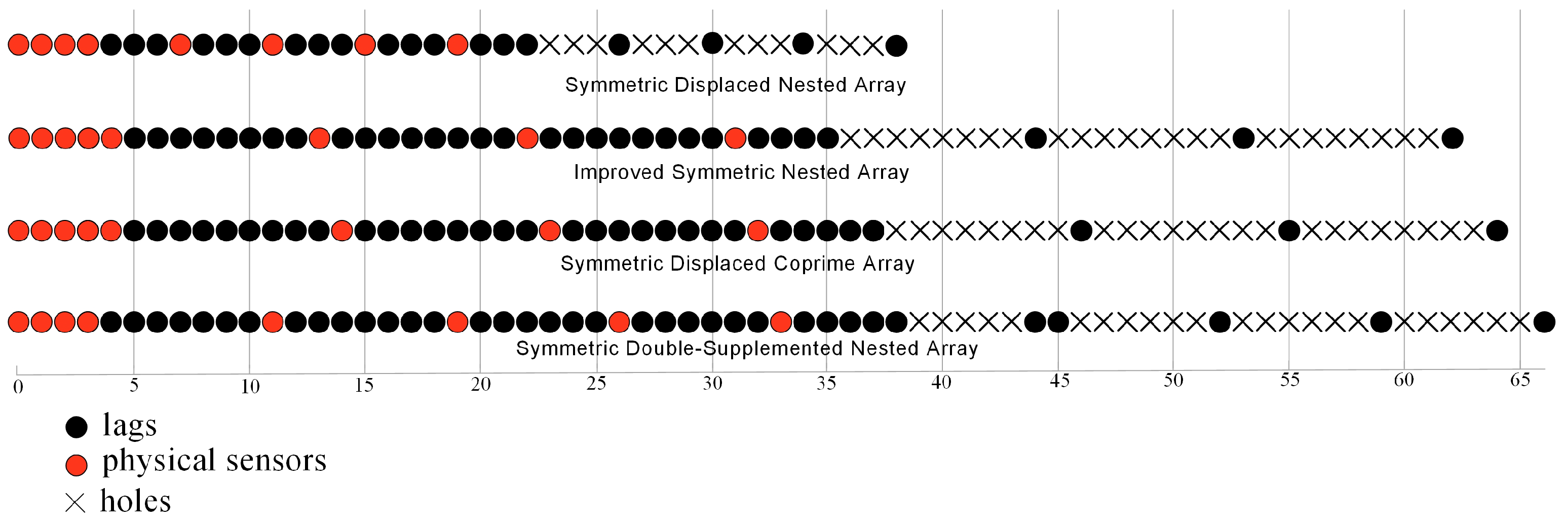
In order to visually describe the involved arrays of the five SNLAs, this subsection provides an example of the fifteen sensor locations of the five SNLAs, as shown in Figure 2. Since the CSNA and ISNA have the same array configuration when the number of sensors is odd, only the array configuration of the ISNA is given in the figure. All of the above arrays are symmetric, i.e., the two sides of the origin are composed of positive locations and negative locations, and only the array configuration of the non-negative part is given on the way. In Figure 2, the horizontal axis reflects the positional relationship between sensors, the red circles denote the physical sensor locations, the black circles denote the lags of the DCAs, and the black crosses denote the holes between the DCAs. The DOF denotes the maximum consecutive lags in the DCA, representing the maximum number of field sources that can be detected simultaneously. The array aperture refers to the maximum diameter of the array in the DCA, which is compared.

On this basis, experiments compare the DOFs and apertures for five SNLAs with sensor numbers ranging from 14 to 49. In Figure 3a, we verify the relationship between the array DOF and the number of sensors. When the number of sensors increases, the DOF becomes more significant and the difference in DOFs between different SNLAs becomes larger. The corresponding DOF follows the order: SDSNA > SDCA > ISNA = CSNA > SDNA. In Figure 3b, the aperture becomes more significant as the number of sensors increases. This introduces a more significant difference with the change in the number of sensors and the aperture follows the order: SDSNA > SDCA > ISNA = CSNA > SDNA. The conclusion above highlights that the ISNA configuration restricts the number of sensors to an odd number; thus, ISNA = CSNA holds for an odd number of sensors.

The experimental results show that the SDSNA outperforms the other SNLAs in terms of the DOFs and apertures under the comparison conditions with the same number of sensors.

4.2. Comparison of Array Coupling Effects

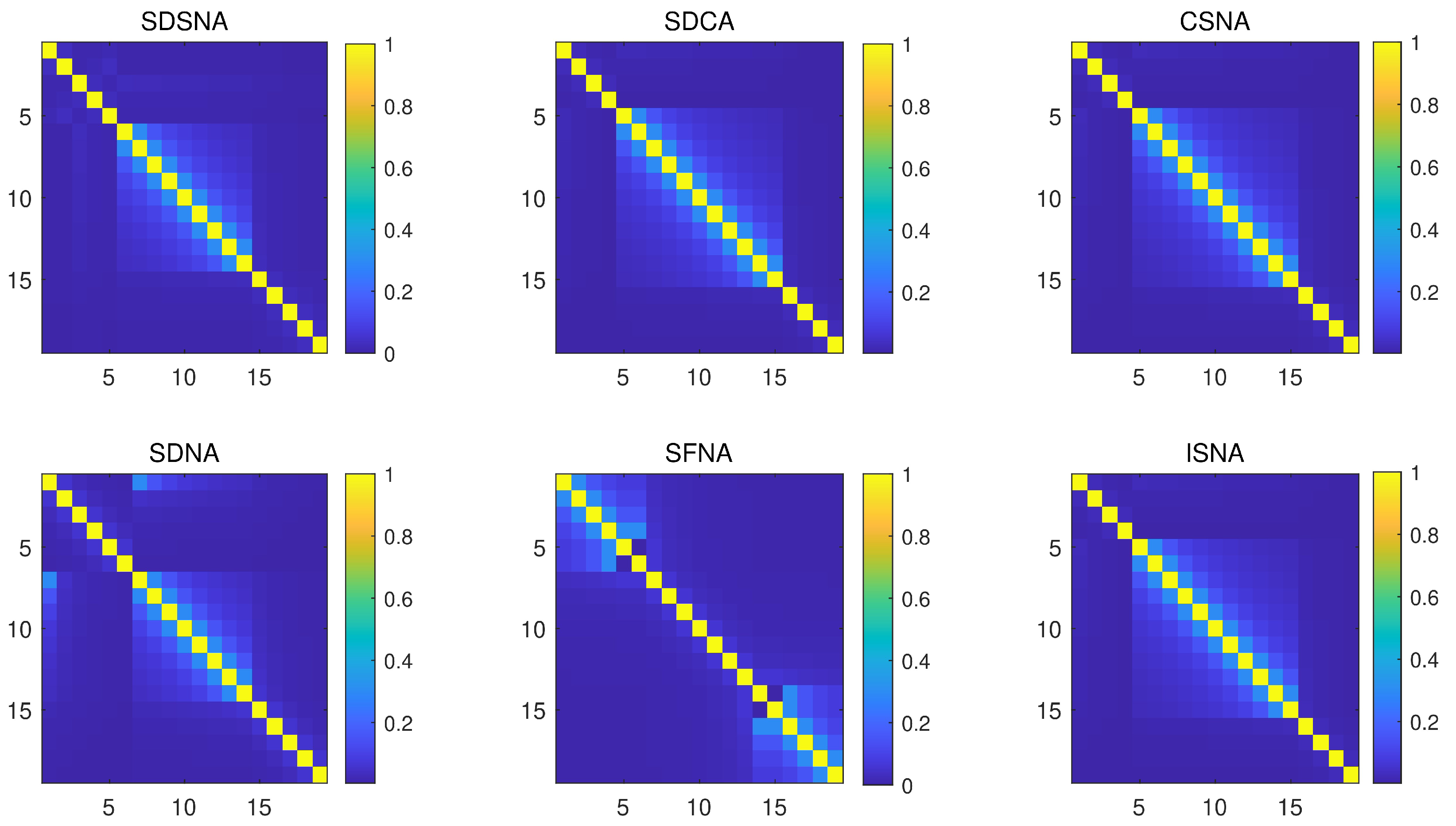
In this section, we focus on the coupling between sensors in the array, which is influenced by the physical distance between the sensors and the array configuration. In order to better illustrate the disparity of coupling effects between different arrays, this experiment will compare two aspects. The experiment is set so that the coupling coefficient $c_1$ is $0.3e^{j\pi /6}$ and $c_i=c_1{e}^{j(i-1)\pi /8}$, where $i=1,2,\dots ,19$. The number of snapshots is 500, with a Monte Carlo experiment repetition of 100 and a signal-to-noise ratio (SNR) of zero.

Firstly, the degree of mutual coupling between the array sensors is investigated by analyzing the coupling matrix amplitude diagram to understand the energy transfer under different SNLAs. In this experiment, five SNLAs—SDCA, CSNA, SDNA, SFNA, and ISNA—were used to experimentally compare the coupling matrix magnitude with the SDSNA. The color of the elements in the coupling matrix amplitude diagram from light to dark indicates their corresponding energies from large to small. The energy transfer state of each array is represented in Figure 4 when the number of array sensors is 19. Compared with the mutual coupling matrix, the coupling matrix amplitude diagram can visualize the energy transfer of each SNLA. In Figure 4, the SDCA, CSNA, and ISNA exhibit a larger area of bright regions compared to the SDSNA, and they are all concentrated in the middle of the array, with an overall larger coupling effect; the SDNA exhibits a smaller area of the central bright region but there is also a bright region at the edge of the coupling matrix amplitude diagram. The bright area energy distribution of the SDSNA is more concentrated in the center of the array. There is no bright area at the edge of the coupling matrix amplitude diagram and the total number of bright areas is small. The SFNA coupling effect is concentrated on both sides of the array element and the coupling of the center array element is minimal, with the overall effect being better than that of the SDSNA. After the experimental comparison, we can conclude that the size of the coupling effect follows the order SDCA ≈ CSNA ≈ ISNA > SDNA > SDSNA > SFNA.

Secondly, based on the coupling matrix amplitude diagram, a quantitative analysis of the coupling effect is carried out experimentally. The coupling effect of the array can be calculated using the known array mutual coupling matrix. The equation is as follows:

$$Leak=\frac{{∥\mathbf{C}-diag\left(\mathbf{C}\right)∥}_F}{{∥\mathbf{C}∥}_F}$$

(85)

where ${∥\ast ∥}_F$ denotes the Frobenius norm of the matrix and, the larger the value $Leak$, the stronger the mutual coupling effect of the array.

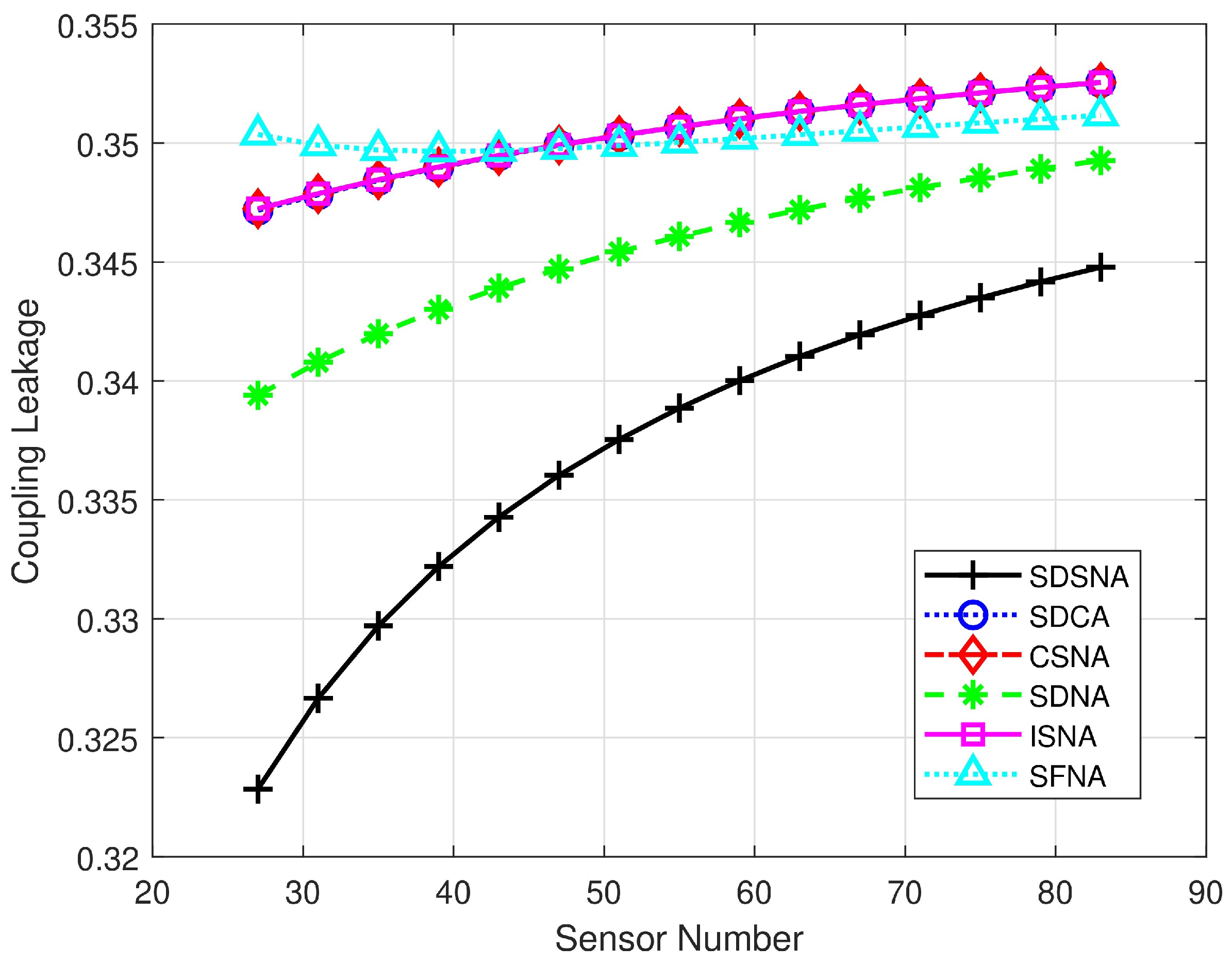
By comparing the coupling leakage of the five SNLAs with the SDSNA in the range of 23 to 83 sensors, the coupling leakage coefficient of the array is derived, as shown in Figure 5. The coupling leakages of the SDCA, CSNA, and ISNA have minimal gaps. The SFNA performs well in the experiment of the coupling matrix amplitude diagram. However, after quantitatively analyzing the coupling leakage values, the overall coupling leakage follows the order: SDCA ≈ CSNA ≈ ISNA > SFNA > SDNA > SDSNA.

The experimental results show that the coupling matrix magnitude diagram can visualize the mutual coupling matrix; however, there are some differences between the observation and the actual coupling effect. A comparison of the coupling leakage values can better reflect the coupling effect of the array and the SDSNA exhibits a lower coupling effect.

4.3. DOA Estimation of Mixed Sources

This subsection applies the DOA and range estimation algorithm using the five SNLAs. The specific performances of the arrays in the localization of mixed-field sources are measured by comparing the RMSE of their estimation results. The RMSE expression is as follows:

$$RMSE=\sqrt{\frac{1}{TL}\sum _{t=1}^T\sum _{i=1}^L{\left({\widehat{y}}_i\left(t\right)-y_i\left(t\right)\right)}^2}$$

(86)

where L is the number of detected sources, T is the number of independent Monte Carlo experiments, ${\widehat{y}}_i\left(t\right)$ is the corresponding estimate for the Tth experiment, and $y_i\left(t\right)$ is the true value of the angle of arrival. The experiments provide basic information about the array and the index set of non-negative parts of sensors in each array is as follows:

$${\mathbb{R}}_{SDSNA}=\{0,1,2,3,4,14,24,33,42\}$$

(87)

$${\mathbb{R}}_{CSNA}=\{0,1,2,3,4,13,22,31,40\}$$

(88)

$${\mathbb{R}}_{SDCA}=\{0,1,2,3,4,14,23,32,41\}$$

(89)

$${\mathbb{R}}_{SDNA}=\{0,1,2,3,4,9,14,19,24,29\}$$

(90)

The corresponding ranges of the five SNLAs for the NF and FF are shown in

Table 3. Array parameters and range of far-field (FF) and near-field (NF) sources.

Name	Number of Sensors	Aperture (d)	NF Lower Bound ($\mathit{\lambda }$)	FF Lower Bound ($\mathit{\lambda }$)
SDSNA	17	84	84.38	1764
CSNA	17	80	78.42	1600
ISNA	17	80	78.42	1600
SDCA	17	82	81.38	1681
SDNA	17	58	48.41	841

.

For the mixed-field source estimation of the array, the experiments are considered in terms of both SNR and snapshot. The experimental results are then obtained.

4.3.1. Comparison of DOA Estimation Performance under Different SNRs

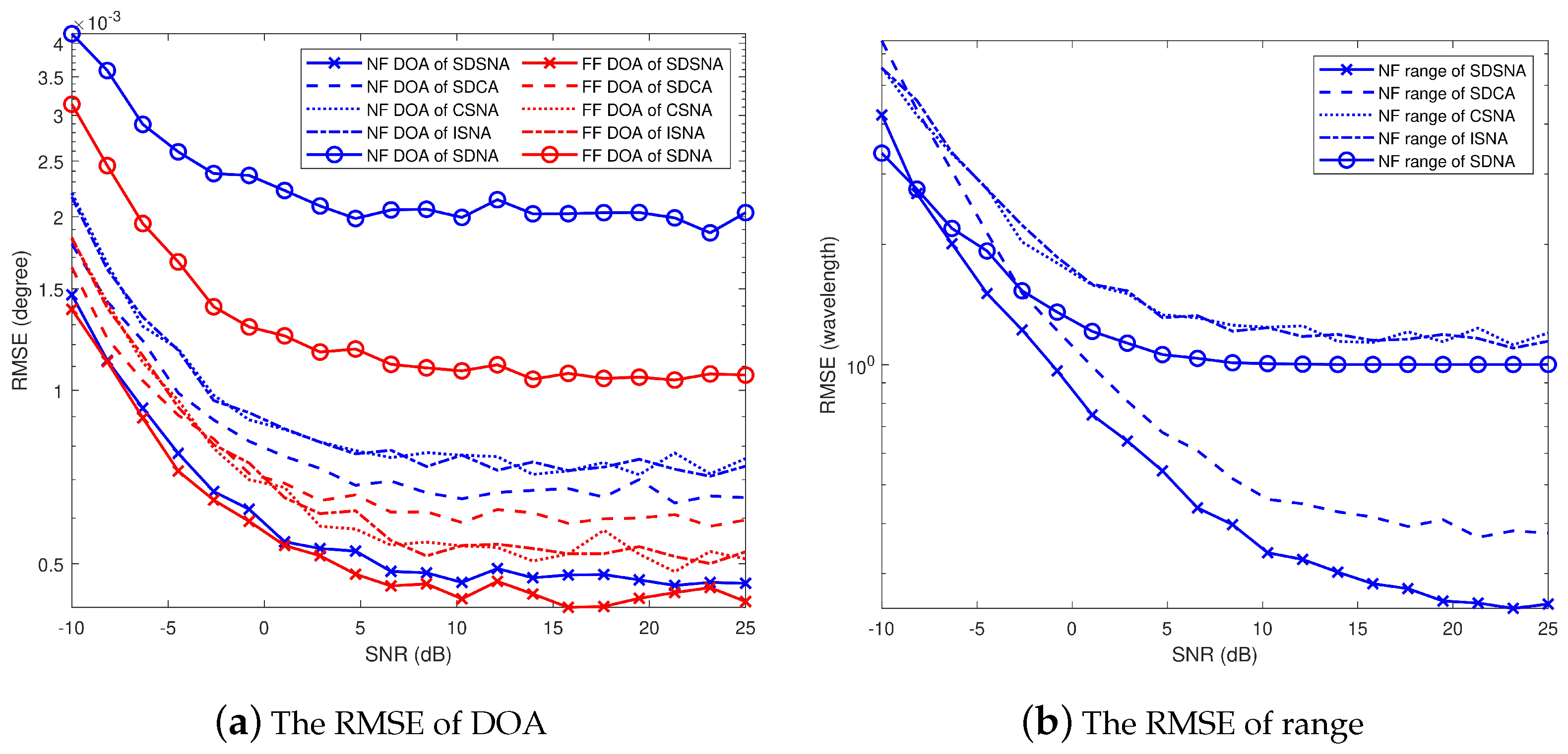
In this experiment, we verify the estimation performance of each array under different SNRs. The interval range of the SNR is $-10$ dB to 25 dB, the number of array sensors is $Q=17$, the sensor interval is $d=\lambda /4$, the number of Monte Carlo experiments is $T=1000$, and the number of snapshots is 1000. By analyzing the range of FF and NF sources in Table 3, we conclude that the common NF source interval of the contrast array is $[84.38\lambda ,841\lambda ]$. We select five source points: three FF source points ($({20}^{\circ },+\infty ),({30}^{\circ },+\infty ),({34}^{\circ },+\infty )$) and two NF source points ($(-{25}^{\circ },440\lambda ),(-{22}^{\circ },450\lambda )$). The selected source points meet the requirements of NF sources, as shown in Table 3.

We experimentally apply the spatial smoothing method and MUSIC algorithm to conduct a performance comparison of an identical number of array sensors and different SNR intervals.

The experimental results are shown in Figure 6a. The RMSE of DOA estimation for the five SNLAs for NF and FF signals are demonstrated. In the figure, the red line indicates the RMSE of DOA for the FF and the blue line indicates the RMSE of DOA for the NF. As the SNR increases, the RMSE of the overall estimation result of the array decreases. Under the condition of a fixed SNR, the SDNA’s estimation performance is the worst, and the SDCA’s estimation results are better than the results of the CSNA and ISNA. However, the performances of the CSNA and ISNA are better in terms of the FF, and the overall RMSE of the SDSNA in the NF and FF is the smallest.

The RMSE of the five SNLAs in estimating the NF signal range is demonstrated in Figure 6b. As the SNR increases, the range estimation of the arrays improves. Under the condition of a fixed SNR, the range estimation error follows the order CSNA > ISNA > SDNA > SDCA > SDSNA. The RMSE of the SDSNA’s range estimation is the smallest. The experimental results show that the SDSNA’s DOA and range estimation perform best over an SNR interval from −10 db to 25 db.

4.3.2. Comparison of DOA Estimation Performance under Different Number of Snapshots

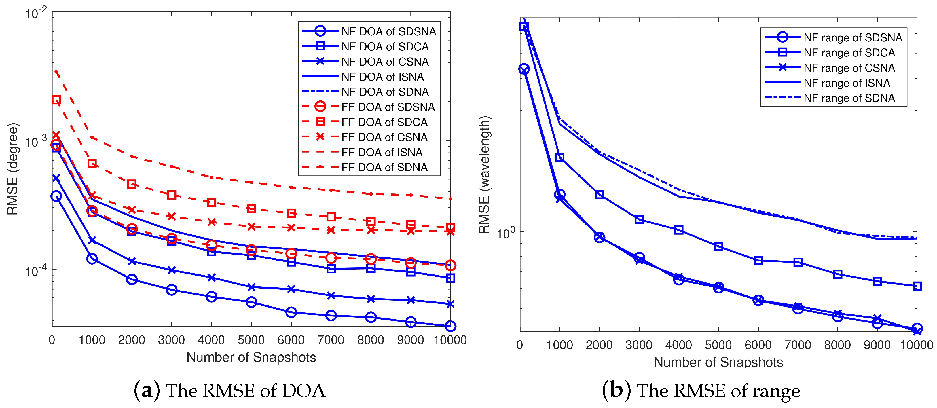
Here, we verify the estimation performance comparison of each array under different snapshots. In this experiment, we set the number of array sensors to $Q=17$, the interval of the sensors to $d=\lambda /4$, the number of Monte Carlo experiments to $T=1000$, the $SNR=10$ dB, and the snapshot selection intervals from 1000 to 10,000. Four source points are selected, which are three FF source points ($({20}^{\circ },+\infty ),({30}^{\circ },+\infty ),({34}^{\circ },+\infty )$) and one NF source point ((−${25}^{\circ },410\lambda )$).

We also experimentally apply the spatial smoothing method and MUSIC algorithm to conduct a performance comparison with the same number of array sensors and different number of snapshots. The performance comparison under different snapshots with the same number of array sensors is shown in Figure 7.

Figure 7a illustrates the RMSE of the NF and FF DOA estimation, wherein the red line indicates the RMSE of the DOA for FF and the blue line indicates the RMSE of the DOA for NF. In the experimental results, it can be seen more clearly that the RMSEs of the NF and FF DOA estimation follow the order SDNA > SDCA > CSNA = ISNA > SDSNA. The SDSNA exhibits better mixed-field source DOA estimation performance in the snapshot range of 1000 to 10,000.

Figure 7b shows the range estimation of the five SNLAs, in which the SDNA and ISNA show similar estimation accuracies, with the ISNA being slightly better than the SDNA. The SDCA exhibits intermediate estimation accuracy, and the SDSNA and CSNA exhibit the best estimation results, with the SDSNA being better than the CSNA in some snapshots. The experimental results show that the SDSNA has a more minor RMSE in range estimation at snapshot lengths between 1000 and 10,000.

5. Discussion

In the field of DOA estimation, the current challenges arise from the limitations of FF source estimations, which do not adequately address real-world applications. These applications often involve multiple sources with indeterminate locations, necessitating the estimation of DOA for mixed-field sources. Traditional methods struggle to separate the FF and NF signal components within the constraints of physical array structures, such as limited apertures and DOF. The SNLA offers significant improvements for DOA estimation of mixed-field sources. Its symmetrical structure simplifies the DOA parameter analysis of NF sources. The non-uniformity of the SNLA enables larger array apertures compared to the SULA with the same number of sensors, thus enhancing accuracy in mixed-field source location and DOA angle resolution. Moreover, the SNLA’s DCA has a virtual array with longer continuous uniform subarrays, affording a higher DOF and the capability of detecting more sources for underdetermined DOA estimation. The SNLA also benefits from lower cost and complexity, achieving a greater DOF with fewer sensors. However, there is still potential to improve the DOF and aperture of existing SNLA arrays and enhance DOA estimation accuracy. A new design, the symmetric double-supplemented nested array (SDSNA), is proposed to address these challenges. This design adds sensor elements to fill holes in the DCA, creating more continuous array structures. The SDSNA surpasses the conventional SNLA in terms of physical array properties, such as aperture, DOF, coupling effect, and DOA estimation accuracy. Performance comparisons between arrays typically consider physical properties and algorithmic applications. As demonstrated in Figure 3, the SDSNA shows superiority in terms of both DOF and aperture compared to the other arrays, indicating its enhanced capability to detect more signal sources with higher accuracy. Figure 4 and Figure 5 compare subjective and objective coupling effects, respectively, revealing minimal coupling leakage for the SDSNA. Finally, after applying the DOA algorithm to the SDSNA and setting appropriate conditions for DOA estimation, the RMSE of the SDSNA under various experimental conditions is lower than that of other arrays, confirming its superior DOA estimation performance. Future research and limitations will include the following:

• In the experiments in Section 4.3, we found that the error introduced by the distance estimation of the array is large when the SNR is low. In the future, we will explore mixed-field source localization at low SNRs to achieve better estimation results.
• We aim to extend this supplemented design approach to optimize array performance and apply specialized array algorithms for mixed-field sources. The ultimate goal is to design both arrays and algorithms that achieve higher precision in DOA estimation.
• This paper concentrates on the design and evaluation of the SDSNA, with its performance validated via simulation experiments. However, it does not include practical field tests. Future work will aim to conduct comprehensive testing and enhance the structural design of the antenna, tailored to specific real-world application contexts.

6. Conclusions

In this study, a symmetrical double-supplemented nested array for mixed NF and FF source localization is proposed. This array integrates a unique nested array configuration with two sets of supplemented sensors. The design utilizes a single supplemented sensor to fill the DCA’s holes, thus expanding the array’s physical aperture. An essential feature of the SDSNA is its representation through a closed-form expression, enhancing its practical applicability and simplifying design processes. One aspect of this study involves the mathematical derivation of the array’s maximum continuous virtual array length. By analyzing the maximum consecutive lag expression, the optimal array configuration is determined, thus ensuring a maximal DOF. The experimental design compares the physical properties of the SDSNA with existing SNLA arrays, demonstrating its superiority in terms of both DOF and aperture size. Additionally, a coupling leakage experiment is conducted, highlighting the unique coupling characteristics of the SDSNA and its advantages in this area. The array’s estimation performance is validated by applying the DOA algorithm. This analysis, conducted with various SNRs and numbers of snapshots, concludes that the SDSNA offers better DOA estimation capabilities. In summary, the SDSNA exhibits better performance in FF and NF direction estimations, as well as NF distance measurements. Its efficacy in the passive detection of mixed-field sources renders it suitable for applications in radar systems, microphone arrays, and military remote sensing auxiliary systems. This array design approach improves performance and expands the range of applications for source localization techniques.

References

1. Krim, H.; Viberg, M. Two decades of array signal processing research: The parametric approach. IEEE Signal Process. Mag. 1996, 13, 67–94. [Google Scholar] [CrossRef]
2. Liu, M.B.; Hu, G.P.; Shi, J.P.; Zhou, H. DOA estimation method for multi-path targets based on TR MIMO radar. J. Eng. 2019, 2019, 461–465. [Google Scholar] [CrossRef]
3. Shen, J.; Yi, J.; Wan, X.; Xie, D.; Cheng, F. Robust DOA estimation for passive radar with target signals mixed in the reference channel. IEEE Geosci. Remote Sens. Lett. 2020, 18, 456–460. [Google Scholar] [CrossRef]
4. Del Rey-Maestre, N.; Mata-Moya, D.; Jarabo-Amores, M.P.; Gómez-del Hoyo, P.J.; Bárcena-Humanes, J.L.; Rosado-Sanz, J. Passive radar array processing with non-uniform linear arrays for ground target’s detection and localization. Remote Sens. 2017, 9, 756. [Google Scholar] [CrossRef]
5. Jiang, S.; Fu, N.; Wei, Z.; Qiao, L.; Peng, X. Sub-Nyquist Spectrum Sensing and DOA Estimation with Space-Time Trilinear Modeling. IEEE Trans. Instrum. Meas. 2023, 72, 6504613. [Google Scholar] [CrossRef]
6. Pan, M.; Liu, P.; Liu, S.; Qi, W.; Huang, Y.; You, X.; Jia, X.; Li, X. Efficient joint DOA and TOA estimation for indoor positioning with 5G picocell base stations. IEEE Trans. Instrum. Meas. 2022, 71, 8005219. [Google Scholar] [CrossRef]
7. Qi, B.; Zhang, H.; Zhang, X. Time-frequency DOA estimation of chirp signals based on multi-subarray. Digit. Signal Prog. 2021, 113, 103031. [Google Scholar] [CrossRef]
8. Xu, F.; Vorobyov, S.A.; Yang, X. Joint DOD and DOA estimation in slow-time MIMO radar via PARAFAC decomposition. IEEE Signal Process. Lett. 2020, 27, 1495–1499. [Google Scholar] [CrossRef]
9. Chazan, S.E.; Hammer, H.; Hazan, G.; Goldberger, J.; Gannot, S. Multi-microphone speaker separation based on deep DOA estimation. In Proceedings of the 2019 27th European Signal Processing Conference (EUSIPCO), A Coruña, Spain, 2–6 September 2019; pp. 1–5. [Google Scholar]
10. Chen, P.; Chen, Z.; Zheng, B.; Wang, X. Efficient DOA estimation method for reconfigurable intelligent surfaces aided UAV swarm. IEEE Trans. Signal Process. 2022, 70, 743–755. [Google Scholar] [CrossRef]
11. Wan, L.; Sun, Y.; Sun, L.; Ning, Z.; Rodrigues, J.J. Deep learning based autonomous vehicle super resolution DOA estimation for safety driving. IEEE Trans. Intell. Transp. Syst. 2020, 22, 4301–4315. [Google Scholar] [CrossRef]
12. Ding, L.; Ström, E.G.; Zhang, J. Degrees of freedom in 3D linear large-scale antenna array communications—A spatial bandwidth approach. IEEE J. Sel. Areas Commun. 2022, 40, 2805–2822. [Google Scholar] [CrossRef]
13. Schmidt, R. Multiple emitter location and signal parameter estimation. IEEE Trans. Antennas Propag. 1986, 34, 276–280. [Google Scholar] [CrossRef]
14. Xu, T.; Wang, X.; Huang, M.; Lan, X.; Sun, L. Tensor-based reduced-dimension music method for parameter estimation in monostatic fda-mimo radar. Remote Sens. 2021, 13, 3772. [Google Scholar] [CrossRef]
15. Roy, R.; Kailath, T. ESPRIT-estimation of signal parameters via rotational invariance techniques. IEEE Trans. Acoust. Speech Signal Process. 1989, 37, 984–995. [Google Scholar] [CrossRef]
16. Lin, J.; Ma, X.; Yan, S.; Hao, C. Time-frequency multi-invariance ESPRIT for DOA estimation. IEEE Antennas Wirel. Propag. Lett. 2015, 15, 770–773. [Google Scholar] [CrossRef]
17. Qian, C. A simple modification of ESPRIT. IEEE Signal Process. Lett. 2018, 25, 1256–1260. [Google Scholar] [CrossRef]
18. Fortunati, S.; Grasso, R.; Gini, F.; Greco, M.S.; LePage, K. Single-snapshot DOA estimation by using compressed sensing. EURASIP J. Adv. Signal Process. 2014, 2014, 120. [Google Scholar] [CrossRef]
19. Shen, Q.; Liu, W.; Cui, W.; Wu, S. Underdetermined DOA estimation under the compressive sensing framework: A review. IEEE Access 2016, 4, 8865–8878. [Google Scholar] [CrossRef]
20. Famoriji, O.J.; Shongwe, T. Source localization of EM waves in the near-field of spherical antenna array in the presence of unknown mutual coupling. Wirel. Commun. Mob. Comput. 2021, 2021, 3237219. [Google Scholar] [CrossRef]
21. Huang, Y.D.; Barkat, M. Near-field multiple source localization by passive sensor array. IEEE Trans. Antennas Propag. 1991, 39, 968–975. [Google Scholar] [CrossRef]
22. Starer, D.; Nehorai, A. Passive localization of near-field sources by path following. IEEE Trans. Signal Process. 1994, 42, 677–680. [Google Scholar] [CrossRef]
23. Challa, R.N.; Shamsunder, S. High-order subspace-based algorithms for passive localization of near-field sources. In Proceedings of the Conference Record of the Twenty-Ninth Asilomar Conference on Signals, Systems and Computers, Pacific Grove, CA, USA, 30 October–1 November 1995; Volume 2, pp. 777–781. [Google Scholar]
24. Abou Chaaya, J.; Picheral, J.; Marcos, S. Localization of spatially distributed near-field sources with unknown angular spread shape. Signal Process. 2015, 106, 259–265. [Google Scholar] [CrossRef]
25. Wu, X.; Chen, H.; Zhu, W.P. A gridless one-step method for mixed far-field and near-field sources localization. Digit. Signal Prog. 2020, 104, 102784. [Google Scholar] [CrossRef]
26. Liang, J.; Liu, D. Passive localization of mixed near-field and far-field sources using two-stage MUSIC algorithm. IEEE Trans. Signal Process. 2009, 58, 108–120. [Google Scholar] [CrossRef]
27. Wang, B.; Liu, J.; Sun, X. Mixed sources localization based on sparse signal reconstruction. IEEE Signal Process. Lett. 2012, 19, 487–490. [Google Scholar] [CrossRef]
28. He, J.; Swamy, M.; Ahmad, M.O. Efficient application of MUSIC algorithm under the coexistence of far-field and near-field sources. IEEE Trans. Signal Process. 2011, 60, 2066–2070. [Google Scholar] [CrossRef]
29. Wang, K.; Wang, L.; Shang, J.R.; Qu, X.X. Mixed near-field and far-field source localization based on uniform linear array partition. IEEE Sens. J. 2016, 16, 8083–8090. [Google Scholar] [CrossRef]
30. Shi, W.; Vorobyov, S.A.; Li, Y. ULA fitting for sparse array design. IEEE Trans. Signal Process. 2021, 69, 6431–6447. [Google Scholar] [CrossRef]
31. Gao, S.; Ma, H.; Liu, H.; Yang, J.; Yang, Y. A Gridless DOA Estimation Method for Sparse SensorArray. Remote Sens. 2023, 15, 5281. [Google Scholar] [CrossRef]
32. Wang, X.; Yang, Z.; Huang, J.; de Lamare, R.C. Robust two-stage reduced-dimension sparsity-aware STAP for airborne radar with coprime arrays. IEEE Trans. Signal Process. 2019, 68, 81–96. [Google Scholar] [CrossRef]
33. Leite, W.S.; de Lamare, R.C. List-based OMP and an enhanced model for DOA estimation with nonuniform arrays. IEEE Trans. Aerosp. Electron. Syst. 2021, 57, 4457–4464. [Google Scholar] [CrossRef]
34. Pal, P.; Vaidyanathan, P.P. Nested arrays: A novel approach to array processing with enhanced degrees of freedom. IEEE Trans. Signal Process. 2010, 58, 4167–4181. [Google Scholar] [CrossRef]
35. Zhao, J.; Gui, R.; Dong, X.; Sun, M.; Wang, Y. Direction of Arrival Estimation with Nested Arrays in Presence of Impulsive Noise: A Correlation Entropy-Based Infinite Norm Strategy. Remote Sens. 2023, 15, 5345. [Google Scholar] [CrossRef]
36. Vaidyanathan, P.P.; Pal, P. Sparse sensing with co-prime samplers and arrays. IEEE Trans. Signal Process. 2010, 59, 573–586. [Google Scholar] [CrossRef]
37. Li, S.; Xie, D. Compressed symmetric nested arrays and their application for direction-of-arrival estimation of near-field sources. Sensors 2016, 16, 1939. [Google Scholar] [CrossRef]
38. Tian, Y.; Lian, Q.; Xu, H. Mixed near-field and far-field source localization utilizing symmetric nested array. Digit. Signal Prog. 2018, 73, 16–23. [Google Scholar] [CrossRef]
39. Zheng, Z.; Fu, M.; Wang, W.Q.; Zhang, S.; Liao, Y. Localization of mixed near-field and far-field sources using symmetric double-nested arrays. IEEE Trans. Antennas Propag. 2019, 67, 7059–7070. [Google Scholar] [CrossRef]
40. Zheng, Z.; Fu, M.; Wang, W.Q.; So, H.C. Symmetric displaced coprime array configurations for mixed near-and far-field source localization. IEEE Trans. Antennas Propag. 2020, 69, 465–477. [Google Scholar] [CrossRef]
41. Su, X.; Hu, P.; Liu, Z.; Liu, T.; Peng, B.; Li, X. Mixed near-field and far-field source localization based on convolution neural networks via symmetric nested array. IEEE Trans. Veh. Technol. 2021, 70, 7908–7920. [Google Scholar] [CrossRef]
42. Liu, C.L.; Vaidyanathan, P. Remarks on the spatial smoothing step in coarray MUSIC. IEEE Signal Process. Lett. 2015, 22, 1438–1442. [Google Scholar] [CrossRef]
43. Grosicki, E.; Abed-Meraim, K.; Hua, Y. A weighted linear prediction method for near-field source localization. IEEE Trans. Signal Process. 2005, 53, 3651–3660. [Google Scholar] [CrossRef]
44. Cicchetti, R.; D’Agostino, F.; Ferrara, F.; Gennarelli, C.; Guerriero, R.; Migliozzi, M. Near-field to far-field transformation techniques with spiral scannings: A comprehensive review. Int. J. Antennas Propag. 2014, 2014, 143084. [Google Scholar] [CrossRef]
45. Wang, M.; Nehorai, A. Coarrays, MUSIC, and the Cramér–Rao bound. IEEE Trans. Signal Process. 2016, 65, 933–946. [Google Scholar] [CrossRef]
46. Wang, B.; Zhao, Y.; Liu, J. Mixed-order MUSIC algorithm for localization of far-field and near-field sources. IEEE Signal Process. Lett. 2013, 20, 311–314. [Google Scholar] [CrossRef]
47. Wang, Y.; Cui, W.; Ba, B.; Quan, M.; Yu, Z. Symmetric flipped nested array for mixed near-field and far-field non-circular source localisation. IET Radar Sonar Navig. 2022, 16, 1752–1760. [Google Scholar] [CrossRef]
Figure 1. Symmetric double-supplemented nested array (SDSNA) geometry.
Remotesensing 16 01027 g001
Figure 2. Sensor locations.
Remotesensing 16 01027 g002
Figure 3. Comparison of degrees of freedom (DOFs) and aperture of five SNLAs when changing the number of sensors.
Remotesensing 16 01027 g003
Figure 4. Comparison of mutual coupling matrix amplitude diagrams of each array.
Remotesensing 16 01027 g004
Figure 5. Comparison of coupling leakage of each array under varying the number of sensors.
Remotesensing 16 01027 g005
Figure 6. Comparison of direction of arrival (DOA) and range of each array under different SNRs.
Remotesensing 16 01027 g006
Figure 7. Comparison of DOA and range of each array under different number of snapshots.
Remotesensing 16 01027 g007