X- and Ku-Band SAR Backscattering Signatures of Snow-Covered Lake Ice and Sea Ice

Abstract

In this work, backscattering signatures of snow-covered lake ice and sea ice from X- and Ku-band synthetic aperture radar (SAR) data are investigated. The SAR data were acquired with the ESA airborne SnowSAR sensor in winter 2012 over Lake Orajärvi in northern Finland and over landfast ice in the Bay of Bothnia of the Baltic Sea. Co-incident with the SnowSAR acquisitions, in situ snow and ice data were measured. In addition, time series of TerraSAR-X images and ice mass balance buoy data were acquired for Lake Orajärvi in 2011–2012. The main objective of our study was to investigate relationships between SAR backscattering signatures and snow depth over lake and sea ice, with the ultimate objective of assessing the feasibility of retrieval of snow characteristics using X- and Ku-band dual-polarization (VV and VH) SAR over freshwater or sea ice. This study constitutes the first comprehensive survey of snow backscattering signatures at these two combined frequencies over both lake and sea ice. For lake ice, we show that X-band VH-polarized backscattering coefficient (${\mathsf{\sigma }}^{\mathrm{o}}$) and the Ku-band VV/VH-ratio exhibited the highest sensitivity to the snow depth. For sea ice, the highest sensitivity to the snow depth was found from the Ku-band VV-polarized ${\mathsf{\sigma }}^{\mathrm{o}}$ and the Ku-band VV/VH-ratio. However, the observed relations were relatively weak, indicating that at least for the prevailing snow conditions, obtaining reliable estimates of snow depth over lake and sea ice would be challenging using only X- and Ku-band backscattering information.

1. Introduction

Snow cover has a major impact on the evolution of ice cover in both lake and sea environments [1,2]. During the freezing season, snow cover introduces a strong insulation effect that reduces ice growth at the ice/water interface. When the ice is thin, a heavy snow load on ice can contribute to the total ice mass by widespread surface flooding that forms slush and later snow-ice [2]. During the melting season, snow meltwater refreezing at the snow/ice interface leads to forming of superimposed ice [2]. Additionally, the high albedo of snow reflects a large part of solar radiation, which alters the surface energy balance and affects the amount of energy being reflected, absorbed, and transmitted through the ice and the underlying water. During the melt season, the ice starts to melt faster after snow melt-off [3].

Accurate snow depth data are needed to model the heat, momentum, and gas fluxes between the ocean, ice, and atmosphere [3]. Furthermore, snow on ice is a significant source of uncertainty in sea ice thickness estimation based on radar and laser altimetry (e.g., CryoSat-2 and ICESat-2) [4,5].

Snow depth on sea and lake ice needs to be observed with spatial and temporal resolutions required by numerical weather prediction models and operational monitoring of the state of lake and ocean conditions, e.g., daily, at 10 km resolution. While accurate data can be obtained with in situ observations, these rarely cover a large spatial extent at any one time. Airborne measurements of snow depth with an airborne Frequency-Modulated Continuous-Wave (FMCW) radar [6,7,8] cover a much larger area than in situ measurements in a short time but are too expensive for continuous monitoring. Improved ultra-wideband radars (UWBs) have also been installed in airplanes to find out the snow depth on the Arctic sea ice [9]. In addition, recently unmanned aerial vehicles (UAVs), known as drones, have been used to retrieve snow depth information on sea ice [10]. One solution is to use satellite microwave remote sensing data for the snow depth estimation on lake and sea ice [11,12].

There are some lake and sea ice properties that have a large influence on the usability of microwave remote sensing instruments to obtain snow and ice information. In the case of lake ice, the water, ice and snow are non-saline, compared to sea ice and its snow cover, which can have a variable degree of salinity. The salinity has a large effect on the relative permittivity of snow and ice and, thus, on the penetration depth of electromagnetic waves. The relative permittivity $\epsilon ={\epsilon }^{\prime }-j{\epsilon }^{\prime \prime }$ is a complex parameter that characterizes the dielectric properties of media, where ${\epsilon }^{\prime }$ is the dielectric constant and ${\epsilon }^{″}$ is the dielectric loss factor. The penetration depth is ${\delta }_p=\sqrt{{\epsilon }^{\prime }}/(k_0{\epsilon }^{\prime \prime })$, where ${\epsilon }^{″}\ll {\epsilon }^{\prime }$ and $k_0$ is the wave number in free space. ${\epsilon }^{″}$ for sea ice is typically higher than for lake ice due to salinity inclusions, reducing the penetration depth greatly, when the frequency is less than 10 GHz [13]. For lake ice, the penetration depth is larger, which results in high-frequency microwave (e.g., 36 and 89 GHz) data to carry snow and ice information from deep ice medium. Ice dynamics, caused by winds and waves, are more substantial in the oceans than in the lakes, leading to drifting of sea ice, ice deformation and variable ice concentration, which yields more variable sensor signatures for sea ice than for lake ice. Over both lake and sea ice close to a coast, the usage of the microwave radiometer (MR) data (resolution 5 to 25 km) is also limited due to mixed-pixel effects (i.e., mixture of land and ice signatures). Finally, the size of most lakes limits the feasibility of using the MR data in estimation of snow depth and other ice and snow properties to only the largest lakes [14].

In this study, we investigate relationships between the snow depth on lake and sea ice and the X- and Ku-band backscattering coefficients (${\mathsf{\sigma }}^{\mathrm{o}}$) from synthetic aperture radar (SAR) imagery. The goal is to see whether snow depth estimation is possible with the ${\mathsf{\sigma }}^{\mathrm{o}}$ data. Retrieval of sea and lake ice properties from X- and Ku-band backscattering was one of the secondary goals of the Cold Regions Hydrology High-Resolution Observatory (CoReH2O), a mission proposal in the ESA Earth Explorer program [15].

The first objective in this paper is to investigate relationships between the snow depth on lake and sea ice and the ${\mathsf{\sigma }}^{\mathrm{o}}$ at the X- and Ku-bands. We use SAR and in situ data collected in Finland, between February and March 2012, during Phase A studies of the CoReH2O mission [15]. The X- and Ku-band SAR data were acquired with ESA’s airborne SnowSAR sensor [16]. Lake ice SAR and in situ data were acquired on Lake Orajärvi, in Northern Finland, and sea ice data on smooth landfast ice in the Bay of Bothnia of the Baltic Sea; see Figure 1. The acquired airborne SAR data are compared with in situ measurements collected along tracks on lake ice and sea ice. In particular, the relationships between spatial variability of snow depth and multi-channel ${\mathsf{\sigma }}^{\mathrm{o}}$ signatures and various ${\mathsf{\sigma }}^{\mathrm{o}}$ polarization ratios are studied. The second objective is to investigate relationships between temporal evolution of snow depth and the ${\mathsf{\sigma }}^{\mathrm{o}}$. This study is conducted using time series of TerraSAR-X (TSX) StripMap Mode images (VV, i.e., vertical–vertical, and VH, i.e., vertical–horizontal polarizations) acquired over the lake ice site in 2011–2012. During this time, an ice mass balance buoy (IMB) collected continuous snow and ice thickness data.

We note that, although there are many other snow and ice properties besides snow depth contributing to the measured ${\mathsf{\sigma }}^{\mathrm{o}}$, such as snow grain size and the size, shape and density of ice air inclusions (i.e., bubbles), here we investigate empirically the relationship between snow depth and the ${\mathsf{\sigma }}^{\mathrm{o}}$. This is due to our interest in seeing if a simple ${\mathsf{\sigma }}^{\mathrm{o}}$ value or ratio-based snow depth estimation is possible with the acquired X- and Ku-band ${\mathsf{\sigma }}^{\mathrm{o}}$ data. We know from past studies that grain size, bubbles, etc., need to be accounted for in order to accurately model the backscattering response; however, from the point of view of operational applications, acquiring any quantitative information on either one is very challenging, especially at high spatial resolution.

This paper is organized as follows. Materials and methods used in this study are first presented in Section 2. The results of our study are presented in Section 3, starting with an overview of snow and ice properties in the sea ice and lake ice sites, and followed by a quantitative analysis of multi-channel SnowSAR ${\mathsf{\sigma }}^{\mathrm{o}}$ data against snow depth on lake and sea ice. Furthermore, a qualitative analysis of TSX imagery for lake ice and the time series of the TSX ${\mathsf{\sigma }}^{\mathrm{o}}$ over lake ice are presented. In Section 4 (Discussion), we compare our results to previous work, and finally, we give our conclusions in Section 5.

2. Materials and Methods

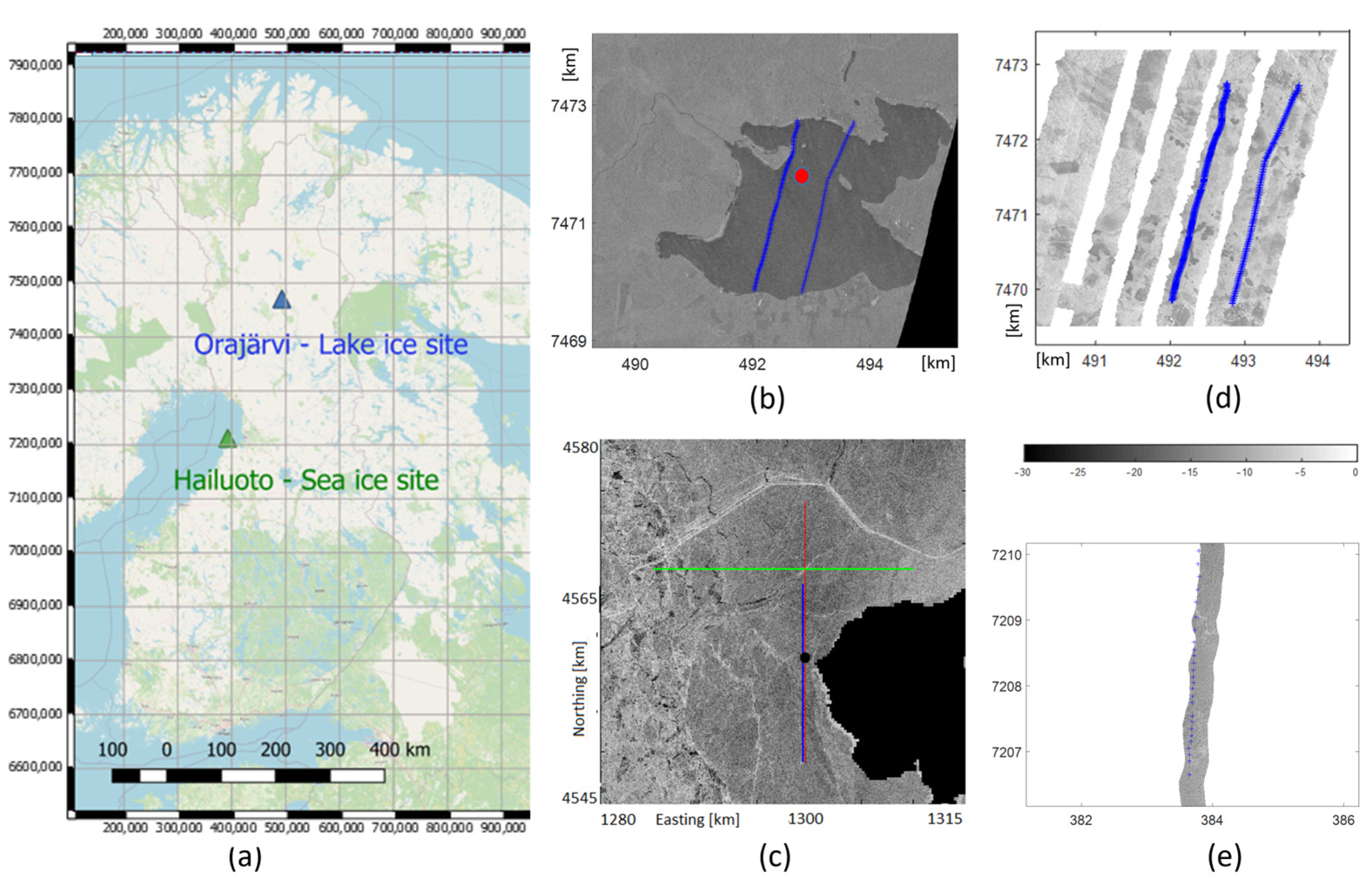
In the following, the study areas for sea ice and lake ice are first presented, followed by descriptions of acquired datasets and their processing for analysis.

2.1. Study Areas

2.1.1. Baltic Sea Landfast Ice Test Site

Sea ice test site was located on smooth landfast ice near Hailuoto Island in the Bay of Bothnia of the Baltic Sea; see Figure 1. The Baltic Sea is a semi-enclosed brackish sea water basin in Northern Europe. The duration of ice season is from five to seven months in the Bay of Bothnia where our test area was located. The upper limit for thermodynamically grown ice is around 70 cm during most winters, the measured maximum being 120 cm [17]. The salinity of the Baltic Sea ice is typically from 0.2 to 2‰, depending on the location, time, and weather history [18].

2.1.2. Lake Orajärvi Test Site

The lake ice test site was located on Lake Orajärvi, in Sodankylä, in Northern Finland; see Figure 1. Lake Orajärvi is a middle-sized (10.95 km²) freshwater lake. Typically, the duration of the ice season is from November/December to May/June (from six to eight months) [19]. The maximum ice thickness usually reaches more than 50 cm in late April [19]. Snow is present on the ice surface every winter season but its spatial distribution is variable across the lake. The mean snow depth and ice thickness during the winter season varied between approximately 2 and 43 cm, and 12 and 69 cm, respectively, in a multiyear study [19].

2.2. Data

2.2.1. Airborne SnowSAR Data

SnowSAR [16] operates simultaneously at the X- (9.6 GHz) and Ku- (17.25 GHz) bands with VV- and VH- polarizations (i.e., XVV, XVH, KuVV and KuVH). SnowSAR imagery was acquired at a spatial resolution of 2 m, swath width of around 400 m and mean antenna look angle of 40° [20]. Noise equivalent ${\mathsf{\sigma }}^{\mathrm{o}}$ is <−28 dB. The radiometric stability of the ${\mathsf{\sigma }}^{\mathrm{o}}$ is <0.5 dB, and the absolute bias is <1 dB.

For the lake ice site, the SnowSAR data (${\mathsf{\sigma }}^{\mathrm{o}}$and elevation angle) from three missions are used here; for mission 2, one flight track in a SAR mosaic acquired on 9 January 2012 close to 14:30, local time (UTC + 2 h); for mission 4, two flight tracks in a mosaic acquired on 7 February 2012 close to 17:00; and for mission 5, one flight track in a mosaic acquired on 22 February 2012 close to 14:00. These flight tracks were approximately 7 km in length. A total of ten SnowSAR data acquisitions were flown over the area (see

Table 1. SnowSAR flight days and in situ dates for each mission and the closest TerraSAR-X image. Missions that are used for analysis in this study are shown with blue color. The dates for in situ data where data cover lake ice area and the dates for SnowSAR flight data in missions 2, 4 and 5, where data cover lake ice area and have in situ data, are marked in bold.

Mission	SnowSAR Flight Date ****	In Situ Date	TSX Date (Closest Image)
1	19 December 2011 20 December 2011	19 December 2011 20 December 2011	17 December 2011
2 *	9 January 2012 10 January 2012	9 January 2012 10 January 2012	8 January 2012
3 *	23 January 2012 24 January 2012	23 January 2012 24 January 2012	30 January 2012
4 *	7 February 2012 8 February 2012	7 February 2012 8 February 2012 9 February 2012 *	10 February 2012
5 *	22 February 2012 23 February 2012	22 February 2012 23 February 2012 24 February 2012	21 February 2012
6 **	26 February 2012	25 February 2012 26 February 2012	21 February 2012
7 ***	1 March 2012	29 February 2012 1 March 2012	3 March 2012
8 ***	5 March 2012	5 March 2012	3 March 2012
9 ***	10 March 2012	8 March 2012 13 March 2012	14 March 2012
10 *	24 March 2012	23 March 2012	25 March 2012

* Snow pits on lake ice; ** No in situ points on lake ice; *** Some in situ points on lake ice (N < 10); **** In situ tracks on lake ice (in the column marked with grey).

). However, there were only three acquisitions (missions 2, 4 and 5) that covered the lake ice areas and had enough coincident in situ data (more than 10 datapoints) to perform an analysis. In the time series analysis, airborne SnowSAR data from all missions (missions from 1 to 10), over Lake Orajärvi, are used.

SnowSAR imagery over the landfast sea ice site was acquired along a 25 km track from south to north near Hailuoto Island; see Figure 1c. The acquisition time was on 8 March 2012 between 13:00 and 14:00, local time.

2.2.2. TerraSAR-X Data over Lake Orajärvi

Over Lake Orajärvi, TSX StripMap Mode imagery at repeat-pass orbits were acquired between October 2011 and May 2012. The total number of images is 23, with a temporal spacing of 11 days. The StripMap images were acquired at VV- and VH-polarizations, with a native resolution of ~2.5 m. For the TSX data, the noise equivalent ${\mathsf{\sigma }}^{\mathrm{o}}$ is typically −22 dB, and the range of incidence angle is from 33.14° to 34.44° [21]. The radiometric stability for TSX is better than 0.15 dB.

2.2.3. In Situ Data on Lake Orajärvi

On Lake Orajärvi, in situ data for mission 2 were acquired on 10 January 2012, one day after the SnowSAR imagery acquisition, along one transect with a length of around 4 km. Snow depth was measured with the Magnaprobe instrument (see http://snowhydro.com, accessed on 9 February 2018) in 269 locations (measured once approximately every 15 m) [22]. Ice thickness, snow density and SWE were measured in five locations. In addition, SWE was measured in three locations. Unfortunately, the closest temporal snow pit measurement was on 8 February.

In situ data for mission 4 were acquired on 8 February 2012, one day after the SnowSAR imagery acquisition, along two transects (denoted as track1 and track2) with a length of around 3 km; see Figure 1d. Snow depth was measured with the Magnaprobe instrument in 254 locations (measured once approximately every 20–30 m) [22]. Ice thickness, snow density and SWE were measured in four locations. In addition, snowpack stratification, snow density, temperature, volumetric wetness (moisture), grain size and grain type profile were measured in a single snow pit on 9 February. A snow fork was used for the moisture measurements.

In situ data for mission 5 were acquired on 22 February 2012, on the same day as the SnowSAR imagery acquisition, along one transect with a length of around 3 km. Snow depth was measured in 1086 locations (measured once approximately every 3–4 m). Ice thickness, snow density and SWE were measured in six locations and mere SWE in two locations. In addition, snowpack stratification, snow density, temperature, moisture, grain size and grain type profile were measured in a single snow pit on 22 February.

Weather data were available from an automatic weather station (AWS) 7.7 km west of the lake ice site in the Sodankylä Arctic Space Centre of the Finnish Meteorological Institute (FMI).

An Ice Mass Balance Buoy (IMB) was deployed on Lake Orajärvi (67 21.704′N, 26 50.047′E; see Figure 1b). The buoy measured a vertical temperature profile from air to water through snow and ice using a thermistor string with 2 cm spacing of sensors. The measurements were conducted four times a day during December 2011–April 2012. The time series of snow depth and ice thickness were derived from the temperature profile data [19].

2.2.4. In Situ Data on Landfast Ice

For the landfast sea ice test site, in situ data were gathered along a transect from south to north from 7–8 March 2012. The length of the transect was 15.2 km. Measured in situ data included snow depth measured once every 100–200 m, SWE and sea ice thickness and freeboard every 1 km. In addition, the scale of local snow depth variation was determined using two 10 m transects with a 1 m sampling interval. Two ice cores were sampled for sea ice salinity determination. The general structure of the snowpack was observed visually. Snow depth was measured either with a measuring rod or a snow scale, while SWE was measured using the snow scale. Weather data were available from the nearby FMI Marjaniemi AWS on Hailuoto Island.

The in situ samples are not completely covered by the SnowSAR acquisition swath. Only about 20 measurement points out of 87 were in the area of the SnowSAR image, covering 2.4 km of the total in situ transect.

2.3. Methods

2.3.1. SnowSAR and TerraSAR-X Data Processing

The SnowSAR images were orthorectified into the UTM35 coordinate reference system and sampled to a 2 m grid. The co-location of the X- and Ku-band SAR images was studied by comparing to other datasets from the area, such as LiDAR data provided by the National Land Survey of Finland and Corine Land Cover classification data provided by the Finnish Environment Institute. The geometric accuracy of the SAR data was found to be within 5 m.

For the sea ice site, ${\mathsf{\sigma }}^{\mathrm{o}}$ data windows of size 5 by 5 pixels around each of the 20 in situ samples covered by the SnowSAR images were extracted. The mean ${\mathsf{\sigma }}^{\mathrm{o}}$ was then calculated for each window. Larger window sizes were also tested, e.g., 50 by 50 (i.e., 100 m × 100 m), but the relation between mean ${\mathsf{\sigma }}^{\mathrm{o}}$ and snow depth was deteriorated for larger windows. The median${\mathsf{\sigma }}^{\mathrm{o}}$ from the window was also tested, but it had a poorer relationship with the snow depth than the mean ${\mathsf{\sigma }}^{\mathrm{o}}$.

For lake ice, an averaging window of size 5 by 5 pixels around each in situ sample was also used. We tested different window sizes, and they had very little influence on the results. It is noted that a larger window would lead to larger spatial averaging of backscattering coefficient data. However, due to some visible artefacts in the SAR images, such as snowmobile tracks from in situ measurements shown as lines of increased ${\mathsf{\sigma }}^{\mathrm{o}}$, the following filtering with the 5 by 5 window was conducted: The average and 1*std (2*std also tested) of the ${\mathsf{\sigma }}^{\mathrm{o}}$ were first calculated. Then, pixels with a ${\mathsf{\sigma }}^{\mathrm{o}}$ value outside the avg ± std (avg ± 2*std also tested) interval were rejected before the final ${\mathsf{\sigma }}^{\mathrm{o}}$ averaging within the 5 × 5 window. In addition, in situ samples too close to an adjacent SnowSAR flight track in the mosaic were eliminated from the calculations.

Compensation of the radar incidence angle was performed using the cosine normalization method in order to reduce the influence of the incidence angle on the mean ${\mathsf{\sigma }}^{\mathrm{o}}$ [23].

$${\sigma }_{{\theta }_{ref}}^o=\frac{{\sigma }^o\blacksquare {\cos }^2{\theta }_{ref}}{{\cos }^2\theta },$$

(1)

where ${\sigma }_{{\theta }_{ref}}^o$ is the normalized ${\mathsf{\sigma }}^{\mathrm{o}}$, ${\mathsf{\sigma }}^{\mathrm{o}}$ is the original backscattering coefficient, $\mathsf{\theta }$is the original incidence angle, and ${\theta }_{ref}$ is the reference angle to which the normalization is conducted. The data were normalized to the reference incidence angles of 43.8° and 43° for the Ku- and X- band data, respectively, as the antennas for the Ku- and X-bands were designed to look at the target at those center angles. In the following Sections, ${\sigma }_{{\theta }_{ref}}^o$ is referred to in short as ${\mathsf{\sigma }}^{\mathrm{o}}$.

The TSX StripMap images that were acquired at VV- and VH-polarizations, with a native resolution of ~2.5 m, were also re-sampled to the 2 m UTM35 grid.

2.3.2. Comparison of SnowSAR Backscatter and In Situ Data

The measured snow depths were compared with the mean ${\mathsf{\sigma }}^{\mathrm{o}}$ values of the SnowSAR bands XVV, XVH, KuVV and KuVH, and various two-channel ratios of the mean ${\mathsf{\sigma }}^{\mathrm{o}}$, e.g., KuVV/XVV, KuVV/KuVH. It is hypothesized that the channel ratios should be more sensitive to the spatial variations in snow depth, as the ${\mathsf{\sigma }}^{\mathrm{o}}$ changes depend on both the polarization and frequency. For example, at the Ku-band, volume scattering from snow is typically assumed to be larger than at the X-band, and backscattering at the VH-polarization is only due to the multiple scattering, but at the VV-polarization single scattering dominates [24]. Over sea ice, the ratios involving the VH-polarization are likely somewhat contaminated by the overall low level of the ${\mathsf{\sigma }}^{\mathrm{o}}$ close to the SnowSAR noise floor (<−28 dB). The investigated relationships between the snow depth and SnowSAR data are characterized by a linear regression fit which was selected instead of higher-order fits due to a large scatter in the datasets.

For the lake ice site, for mission 4, the dependencies were investigated for the two SnowSAR tracks separately. This is due to different incidence angles between them. Although the data were compensated for the same incidence angle, the overlapping areas of the transects may have different ${\mathsf{\sigma }}^{\mathrm{o}}$ vs. snow depth relationships due to differing measurement geometries. In addition, results for the combined tracks were given.

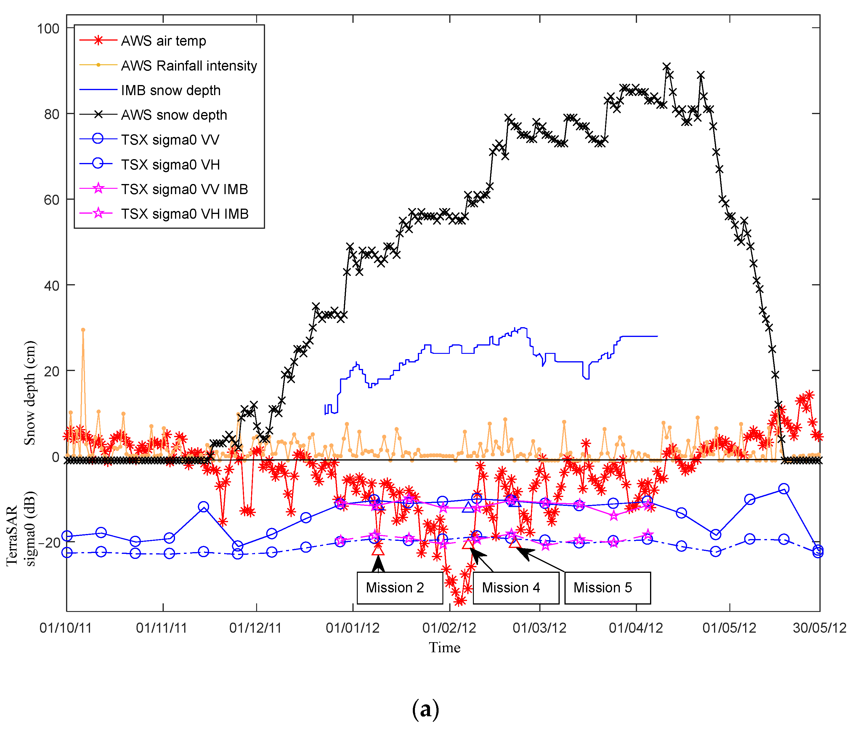
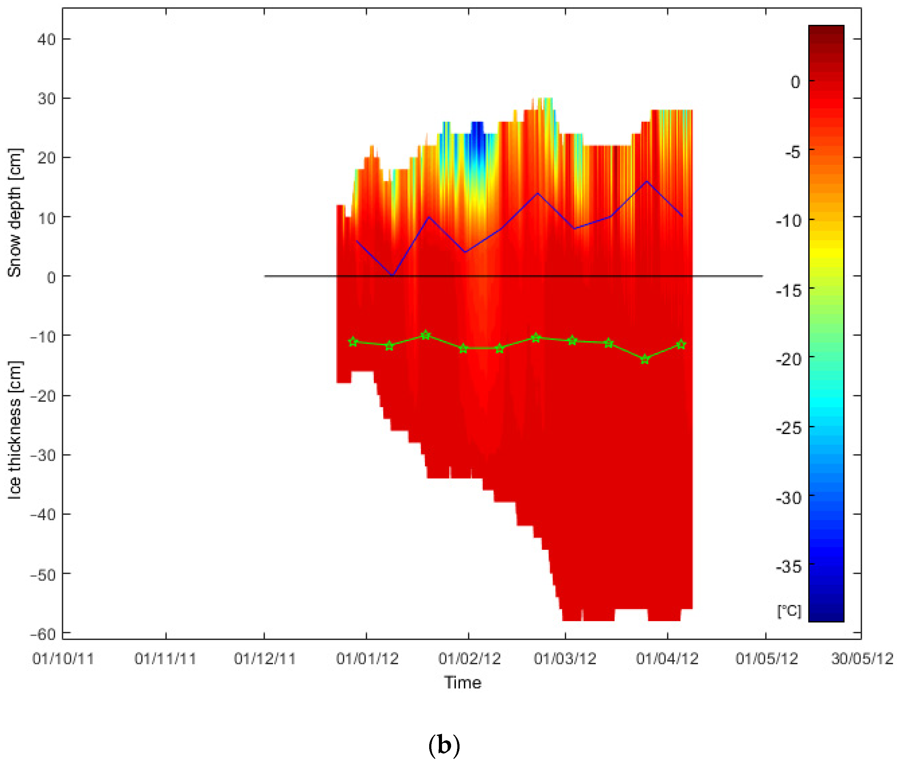
2.3.3. TerraSAR-X and Ice Mass Balance Buoy Data

The changes in the average ${\mathsf{\sigma }}^{\mathrm{o}}$ values of Lake Orajärvi were investigated qualitatively from the TSX images. The temporal evolution of the average ${\mathsf{\sigma }}^{\mathrm{o}}$ value of the entire lake was analyzed and compared visually with the TSX images. The average ${\mathsf{\sigma }}^{\mathrm{o}}$ was calculated from the area covered by Lake Orajärvi in each TSX image by using a mask from Corine data.

The time series of the TSX ${\mathsf{\sigma }}^{\mathrm{o}}$ data from the IMB location and the IMB snow depth data were used to investigate relationships between the temporal evolution of the snow depth and the ${\mathsf{\sigma }}^{\mathrm{o}}$.

In addition, the time series of air temperature, rainfall intensity and snow depth data from the closest AWS were added to the analysis to be able to compare their trends with the TSX ${\mathsf{\sigma }}^{\mathrm{o}}$ and IMB snow depth from 1 October 2011–30 May 2012. The time series of the IMB temperature fields inside the snow and lake ice as well as the average temperature inside the snowpack as a function of time were also calculated. The time series of different temperature layers inside the snowpack were studied in relation with the TSX ${\mathsf{\sigma }}^{\mathrm{o}}$ time series.

3. Results

Here, we present first an overview of snow and ice properties in the sea ice and lake ice sites. Next, relationships between the SnowSAR data and the snow depth on lake ice and sea ice are investigated and quantified. This is followed by qualitative analysis of the TSX imagery for lake ice and analysis of the lake ice TSX ${\mathsf{\sigma }}^{\mathrm{o}}$ time series.

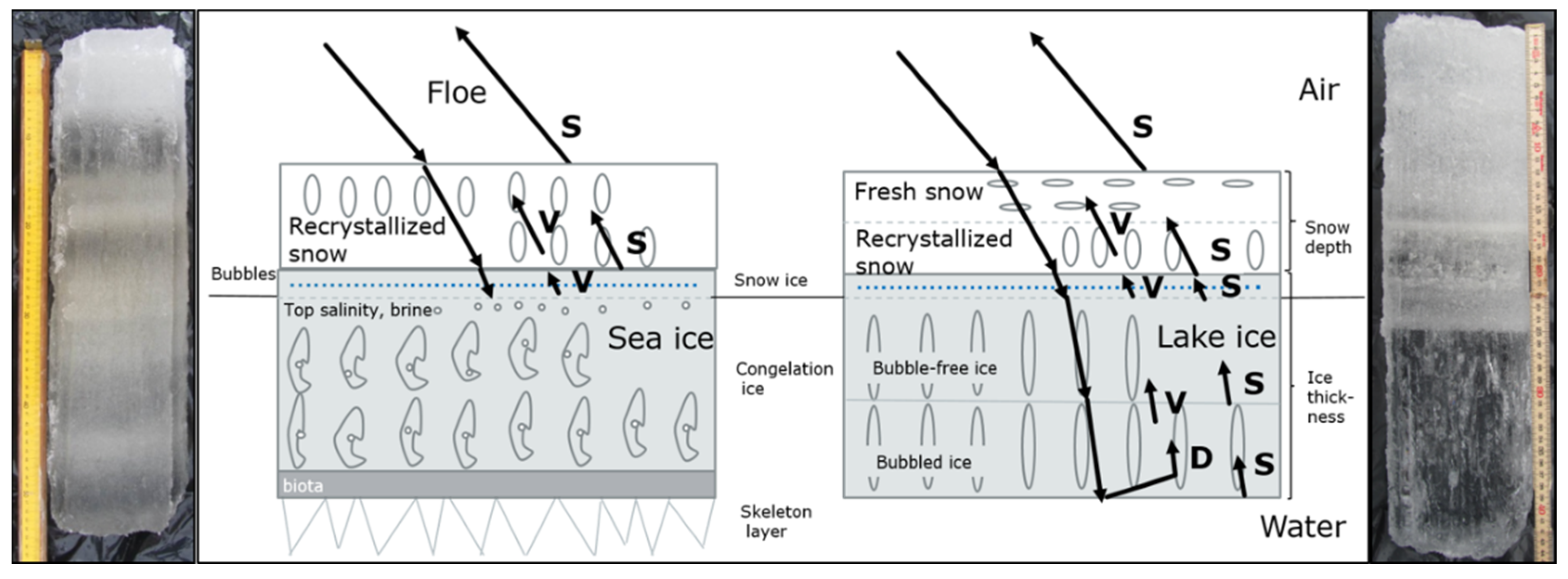
3.1. Overview of Snow and Ice Properties in the Sea Ice and Lake Ice Sites

Various snow and ice properties—snow depth, ice thickness, ice salinity, SWE and snow density—are listed in

Table 2. Statistics of snow and ice properties for the sea ice site.

Sea Ice	Snow and Ice Properties
	Variation	Mean	Std
Snow depth (cm) *	1–37 (2–19) **	14 (11)	7.4 (5.1)
Ice thickness (cm)	29–52	35	5.4
Ice salinity (ppt)	0.2–1.0	-	-
SWE (mm)	16–95 (25–44)	-	-
Snow density (g/cm3)	0.28–0.36 (0.28–0.34)	0.33	0.03

* The STD from local snow depth measurements of two 10 m snow depth transects measured at 1 m spacing was 9.3 cm; i.e., they showed a large local variation in snow depth. ** Parentheses enclose the values for only that part of the in situ transect where coincident SnowSAR data were available.

for the sea ice and in

Table 3. Statistics of snow and ice properties for the lake ice site. For lake ice, the values are from the data where coinciding SnowSAR data were available.

Lake Ice	Snow and Ice Properties
	Variation	Mean	Std
Mission 2
Snow depth (cm)	0.4–27	13	5.1
Ice thickness (cm)	20–30	25	3.8
Mission 4
Track1
Snow depth (cm)	14–35	22 [21] ***	4.1 [4.1]
Ice thickness (cm)	38–40	39	1.0
Track2
Snow depth (cm)	11.5–32	20	3.9
Ice thickness (cm)	-	-	-
Mission 5
Snow depth (cm) Ice thickness (cm)	21–41 37–40	30 39	3.5 1.0

*** Square brackets enclose the values for the track1 and track2 combined.

for lake ice sites.

For the sea ice site, although the snow depth exhibited large spatial variability (compared to the mean), the average snowpack was relatively thin, only 11 cm. The snow and ice thickness in the sea ice site were within a typical range for the landfast ice in the Bay of Bothnia in early March [25]. The variation of snow density was within expected values for settled snow (0.2 to 0.3 g/cm³) and wind-packed snow (0.35 to 0.4 g/cm³) [26]. Based on the in situ observations, the structure of the snowpack was fairly homogeneous. There was a ca. 3 cm layer of hard crust on top with a layer of fine-grained dry snow underneath. The snow was not frozen to the ice surface, but loose. The two sampled ice cores showed vertical salinity variations between 0.2 and 1.0 ppt, which are typical low-salinity values for sea ice in the Bay of Bothnia [18]. According to the AWS observations a few kilometers from the measurement line, the air temperature ($T_a$) was on average −3.7 °C during the SnowSAR data acquisition over the sea ice site on 8 March, and from −6.1 °C to −2.7 °C during the in situ measurement campaign 7–8 March (−8 °C during the night between). The snowpack on the sea ice was qualitatively observed to be dry (i.e., volumetric wetness close to 0%).

For the lake ice site, in mission 2, snow depth varied between 0.4 and 27 cm. According to the AWS data, $T_a$ was about −24 °C during the SnowSAR data acquisition on 9 January (daily mean −20.4 °C), and during the in situ measurement campaign on 10 January the daily mean $T_a$ was −12.6 °C. Based on the snow pit measurements on 8 December 2011 (the closest one for mission 2), snow depth was 7 cm, the temperature of snow was between 0.4 (bottom) and −1.3 °C (top), the density was between 0.13 and 0.15 g/cm³, grain size approximately between 0.5 and 1.5 mm, and grain type was precipitation particles/needle on top and rounded grains/irregular on bottom part of the snow cover.

For the lake ice site, in mission 4, snow depth varied between 12 and 35 cm. $T_a$ was about −29 °C during the SnowSAR data acquisition on 7 February (daily mean −31 °C), and during the in situ measurement campaign on 8 February the daily mean $T_a$ was −26 °C. Based on the snow pit measurements on 9 February, snow depth was 20 cm, the temperature of snow was between −1.9 (bottom) and −17.4 °C (top), the density was between 0.05 and 0.21 g/cm³, moisture between 0.4 and 1.0%, grain size approximately between 0.8 and 2.5 mm, and grain type was precipitation particles/stellars/dendrites/irregular on top and hollow cups on bottom part of the snow cover. The measured snow density values are typical for the site [27].

For mission 5, snow depth varied between 21 and 41 cm. $T_a$ was about −6 °C during the SnowSAR data acquisition on 22 February, and during the in situ measurement campaign on 22 February the daily mean $T_a$ was −9.6 °C. The snow pit measurements on 22 February showed a snow depth of 30 cm. The temperature of the snow was between −0.3 (bottom) and −13.9 °C (top), the density was between 0.14 and 0.24 g/cm³, moisture 1%, grain size approximately between 0.5 and 2 mm, and grain type was partly decomposed precipitation particles on top and hollow cups on the bottom part of the snow cover.

$T_a$ values during the SnowSAR flights and in situ data collection had the largest difference in mission 2, where the former was approximately −20.4 °C and the latter −12.6 °C. For mission 4, $T_a$ values were −31 and −26 °C (for track1), respectively. The SnowSAR and in situ data for mission 5 were acquired on the same day; thus, $T_a$ values were quite similar.

In the IMB time series from December 2011 to April 2012, the snow depth varied between 10 and 30 cm. The ice thickness varied between 16 and 58 cm.

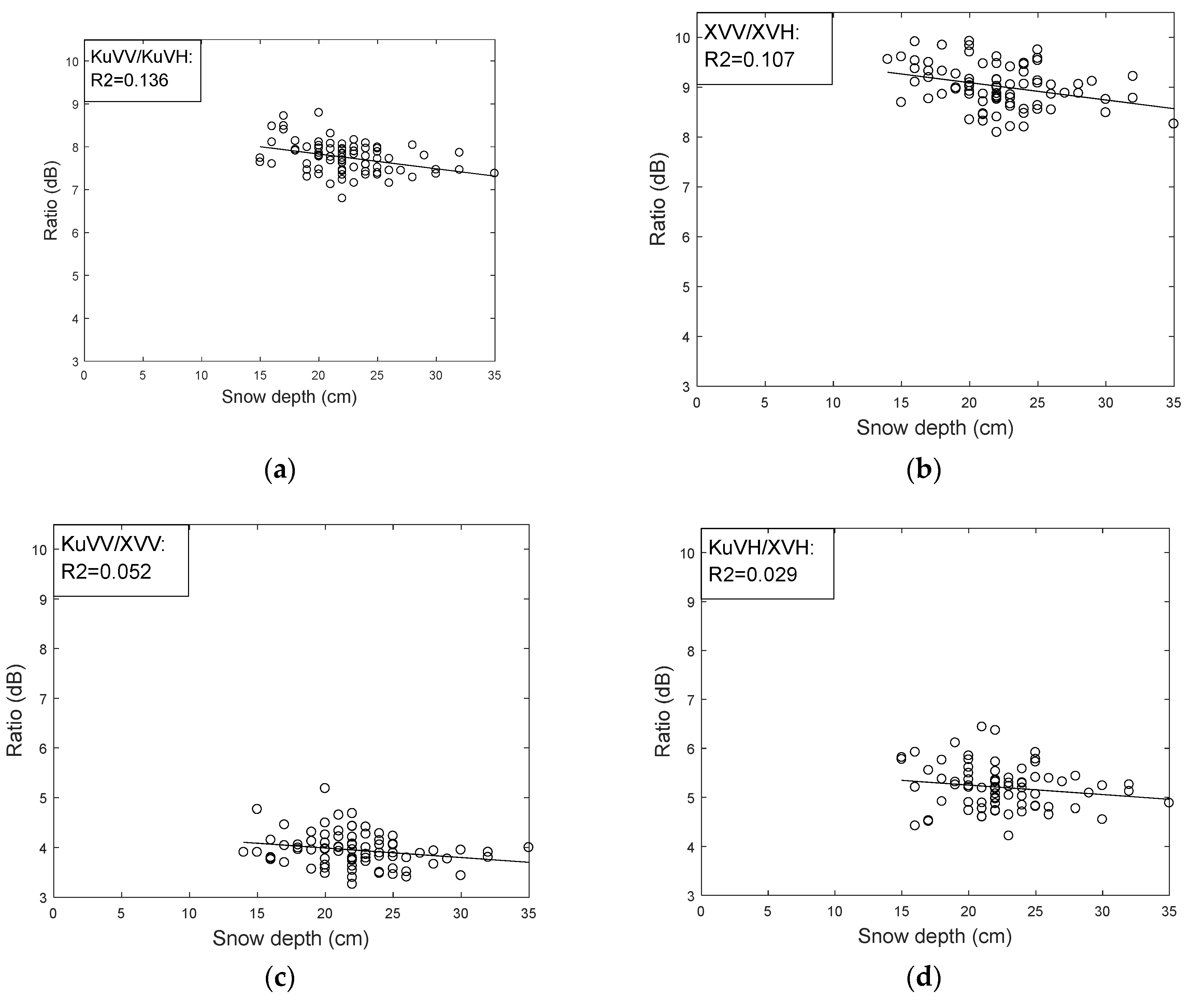
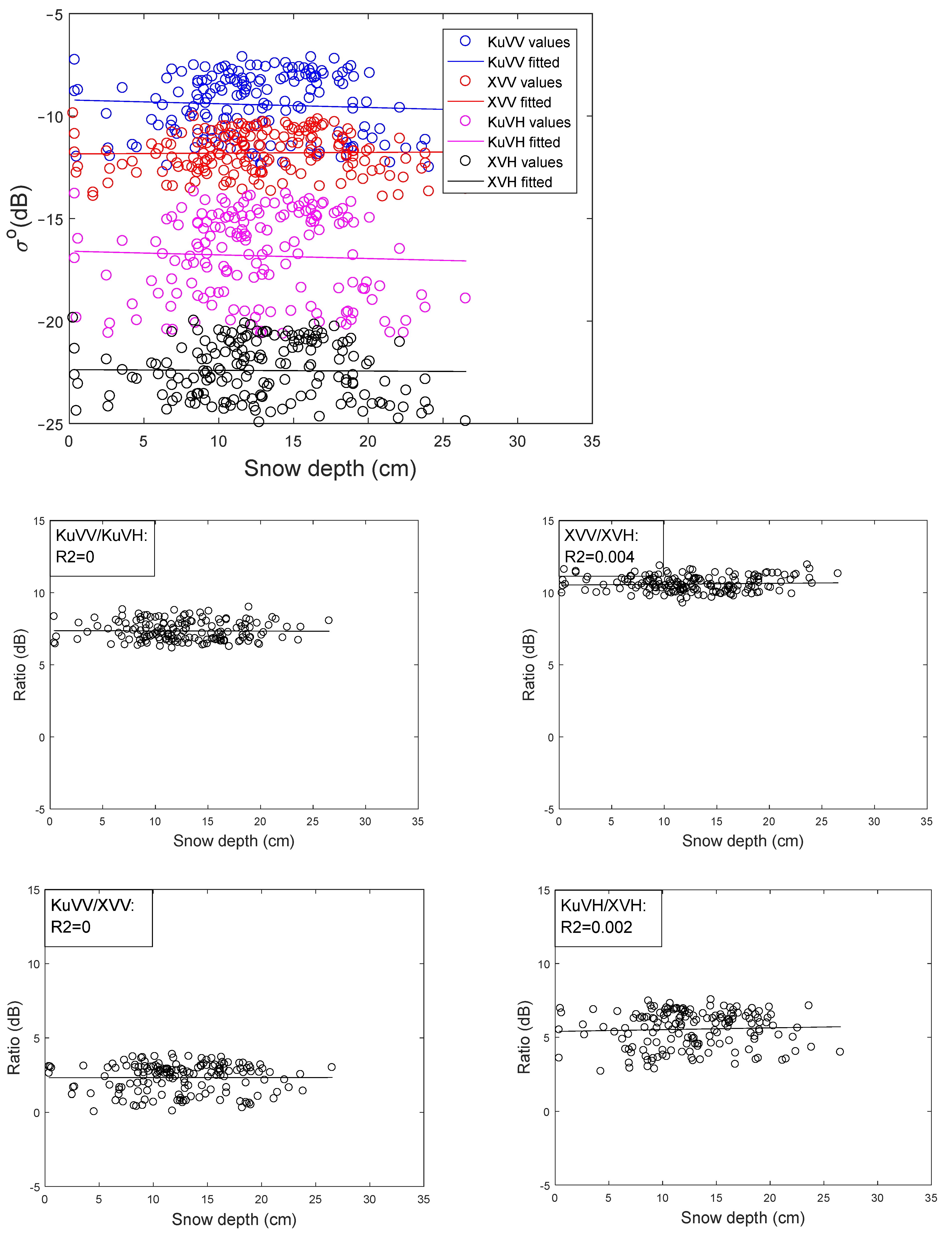
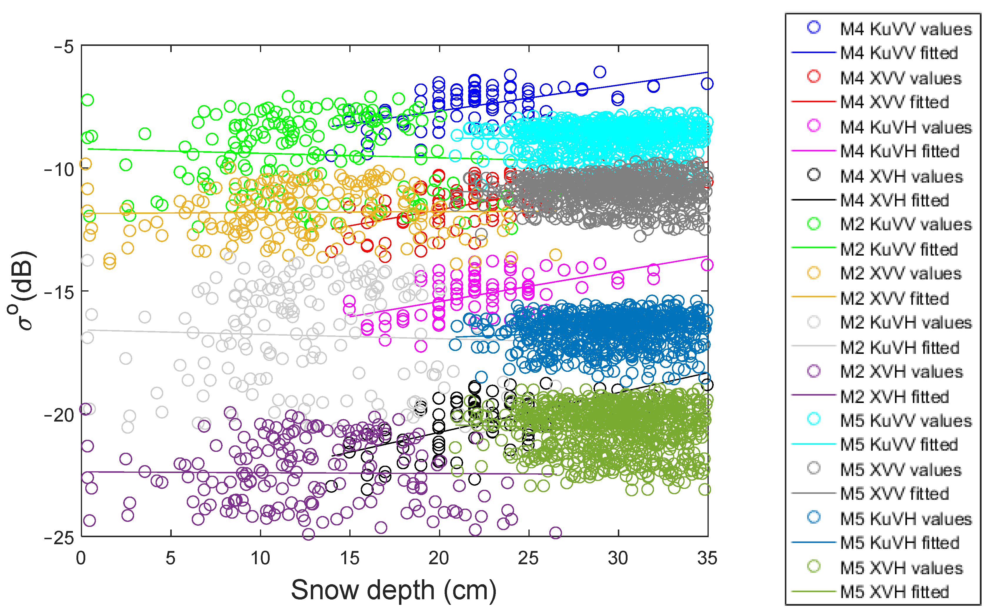
3.2. SnowSAR Data versus Snow Depth on Lake Ice

The relation between the mean ${\mathsf{\sigma }}^{\mathrm{o}}$ and the snow depth for the two measurement lines (track1 and track2 in mission 4) was investigated separately. Figure 2 shows scatterplots between the snow depth and the mean ${\mathsf{\sigma }}^{\mathrm{o}}$ at the four SnowSAR channels. Figure 3 has scatterplots between the SnowSAR channel ratios and snow depth for track1. Linear regression fits to the data are also depicted in the figures. Statistics describing the linear regression between the ${\mathsf{\sigma }}^{\mathrm{o}}$ channels or channel ratios and the snow depth for track1, track2 and for both tracks combined are presented in

Table 4. Statistics of the linear regression between the SnowSAR backscattering coefficient data and the in situ snow depth data for mission 4 track1, track2 and both tracks combined in the lake ice site.

	Slope Term [db/cm]	Average [db]	R2	p-Value
Lake Track1
XVV	0.13	−11.3	0.34	<0.001
XVH	0.16	−20.3	0.36	<0.001
KuVV	0.11	−7.4	0.33	<0.001
KuVH	0.12	−15.1	0.33	<0.001
KuVV/KuVH	−0.03	7.8	0.14	<0.001
XVV/XVH	−0.03	9.0	0.11	0.003
KuVV/XVV	−0.02	4.0	0.05	0.042
KuVH/XVH	−0.02	5.2	0.03	0.138
Lake Track2
XVV	0.08	−12.7	0.15	<0.001
XVH	0.16	−21.1	0.24	<0.001
KuVV	0.08	−8.5	0.19	<0.001
KuVH	0.12	−14.3	0.22	<0.001
KuVV/KuVH	−0.04	6.0	0.09	<0.001
XVV/XVH	−0.07	8.6	0.07	<0.001
KuVV/XVV	−0.01	4.3	0.01	0.142
KuVH/XVH	−0.04	6.8	0.06	0.002
Tracks combined
XVV	0.12	−12.2	0.26	<0.001
XVH	0.16	−20.8	0.29	<0.001
KuVV	0.11	−8.1	0.27	<0.001
KuVH	0.10	−14.6	0.18	<0.001
KuVV/KuVH	−0.00	6.6	0.00	0.722
XVV/XVH	−0.03	8.7	0.02	0.016
KuVV/XVV	−0.02	4.2	0.06	<0.001
KuVH/XVH	−0.05	6.3	0.08	<0.001

.

For track1, the coefficient of determination (R2) between the KuVV ${\mathsf{\sigma }}^{\mathrm{o}}$ and snow depth was modest, 0.33, but the p-value for the regression was <0.001. The coefficient of determination is the same as R2 = r², where r is the coefficient of correlation. For track2, R2 in the case of the KuVV ${\mathsf{\sigma }}^{\mathrm{o}}$ was only 0.19. In general, the results for track2 show R2 values lower than for track1, possibly because track2 exhibited (by visual analysis of the SAR imagery) a wider variety of different lake ice types (mainly refrozen ice from cracks and leads).

The best sensitivity to the snow depth with all channels, in terms of R2, was found for the XVH ${\mathsf{\sigma }}^{\mathrm{o}}$ (R2 = 0.36 for track1 and R2 = 0.24 for track2), and within all channel ratios for the KuVV/KuVH ratio (R2 = 0.14 for track1, R2 = 0.09 for track2). For the combined tracks, the best sensitivity was again for the XVH (R2 = 0.29), but now for the KuVH/XVH ratio (R2 = 0.08). At XVH, the ${\mathsf{\sigma }}^{\mathrm{o}}$ was found to increase more in relation to the snow depth (0.16 dB/cm for track1 and track2, and for the combined tracks) than at other channels.

Additional quick tests were conducted for images (5 × 5 mean averages) for missions 2, 4 and 5 (see

Table 5. Statistics of the linear regression between the SnowSAR backscattering coefficient data and in situ snow depth for missions 2, 4 and 5 (based on quick analysis).

	Mission 2				Mission 4
Polarization	R2	p-Value	Slope Term [db/cm]	Deviation	R2	p-Value	Slope Term [db/cm]	Deviation
XVV	0.04	0.009	−0.058	0.0221	0.26	<0.001	0.2089	0.0223
XVH	0.04	0.016	−0.066	0.0275	0.37	<0.001	0.2608	0.0216
KuVV	0.06	0.002	−0.099	0.0317	0.25	<0.001	0.1899	0.0207
KuVH	0.05	0.005	−0.113	0.0398	0.24	<0.001	0.1714	0.0190
KuVV/KuVH	0.01	0.224	0.013	0.0102	0.01	0.230	0.0185	0.0154
XVV/XVH	0.01	0.201	0.010	0.0076	0.04	0.001	−0.0519	0.0158
KuVV/XVV	0.04	0.016	−0.042	0.0171	0.03	0.005	−0.0190	0.0067
KuVH/XVH	0.03	0.039	−0.047	0.0225	0.14	<0.001	−0.0894	0.0138
	Mission 5
XVV	0.00	0.770	−0.003	0.0110
XVH	0.00	0.044	−0.024	0.0130
KuVV	0.00	0.397	−0.012	0.0144
KuVH	0.00	0.440	−0.012	0.0158
KuVV/KuVH	0.00	0.996	0.000	0.0046
XVV/XVH	0.02	<0.001	0.021	0.0055
KuVV/XVV	0.00	0.045	−0.012	0.0062
KuVH/XVH	0.00	0.213	0.009	0.0074

). For mission 4, similar but somewhat different relations were found compared to the previous ones, due to the more simple analysis performed here (e.g., no angle compensation or std filtering used). However, none of the investigated relations between the SnowSAR channels or channel ratios were found to be statistically significant.

Finally, a similar analysis was conducted for missions 2 and 5 as was conducted for mission 4 in Figure 2 and Figure 3. The results are presented in Appendix A. Figure A4 in Appendix A shows that the best correlation can be found in mission 4. The datasets in different missions differ in the sense that the snow depths cover different ranges. The snow depths in mission 2 include mostly small values, mission 5 large values and mission 4 intermediate values.

The level of backscattering in mission 5 is lower than in mission 4, especially at the Ku-band. The correlation seems to be better between approximately 14–25 cm than with smaller or larger snow depths. The reason could be that, in small snow depths, the effect of ice under the snow dominates, and in larger snow depths the double-bounce effect from the bottom of the ice is lost.

In mission 4, the standard deviation of ice thicknesses is smaller (approximately 1 cm; see Table 3) than in mission 2 (approximately 4 cm), suggesting that the ice could be more like level ice and the surface roughness might not be as large as in mission 2.

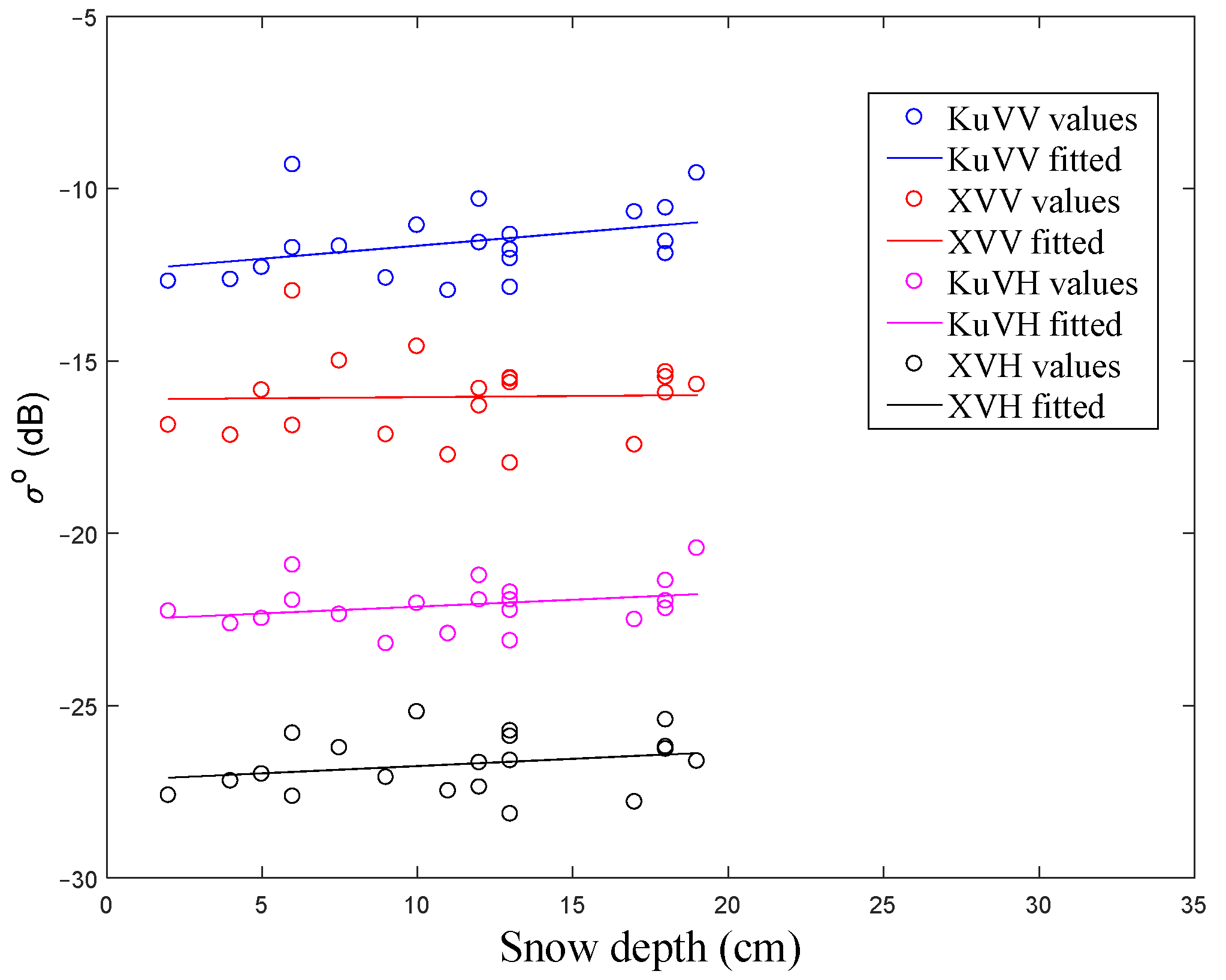
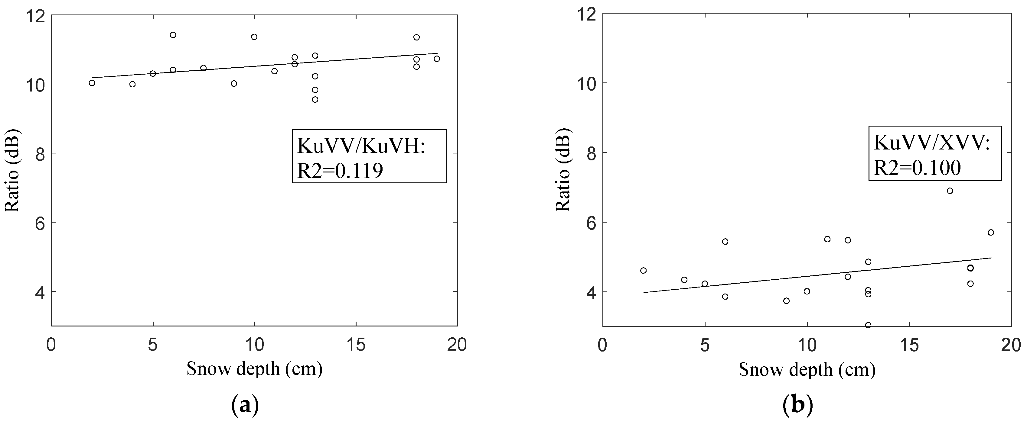
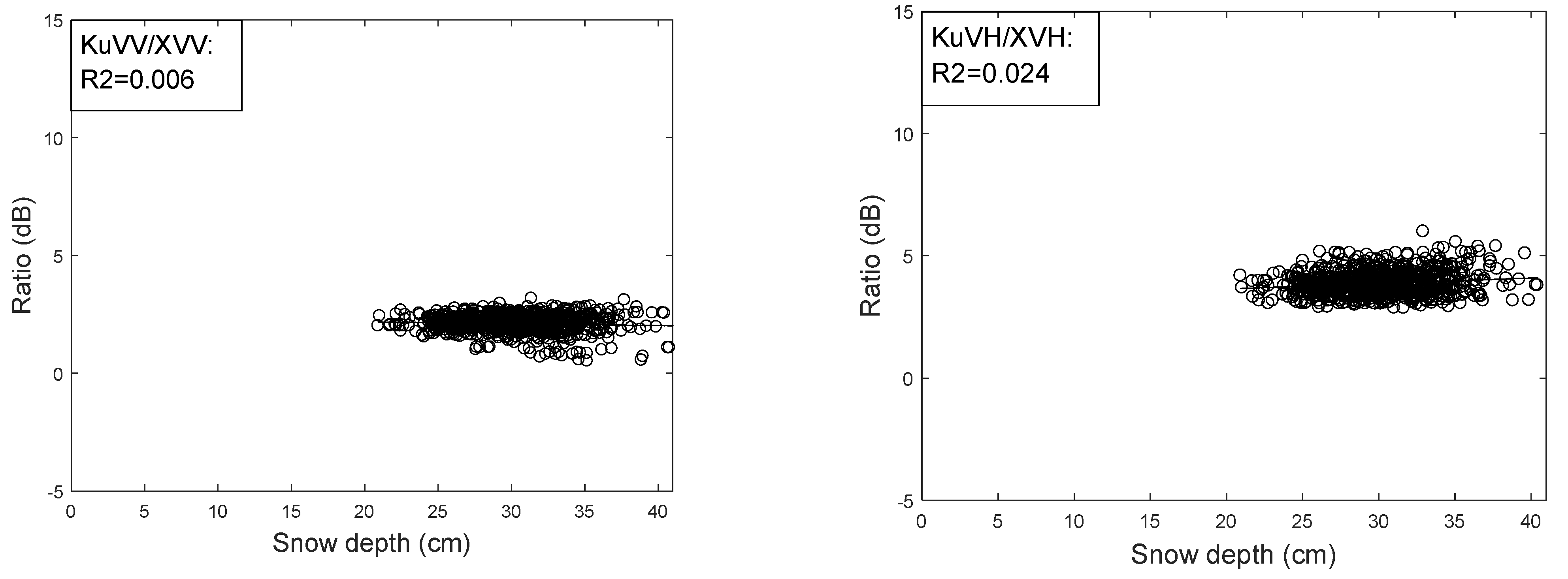
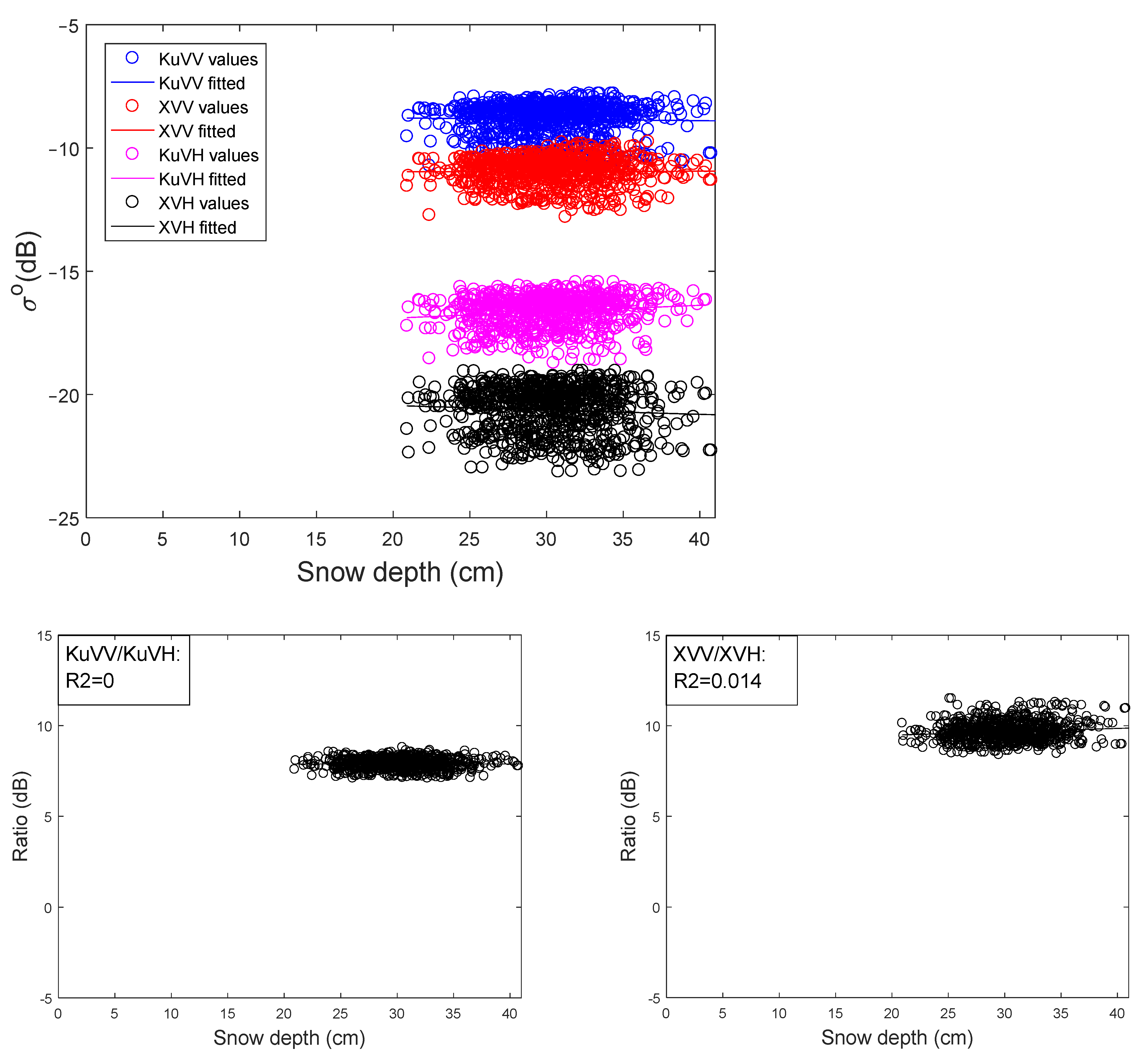
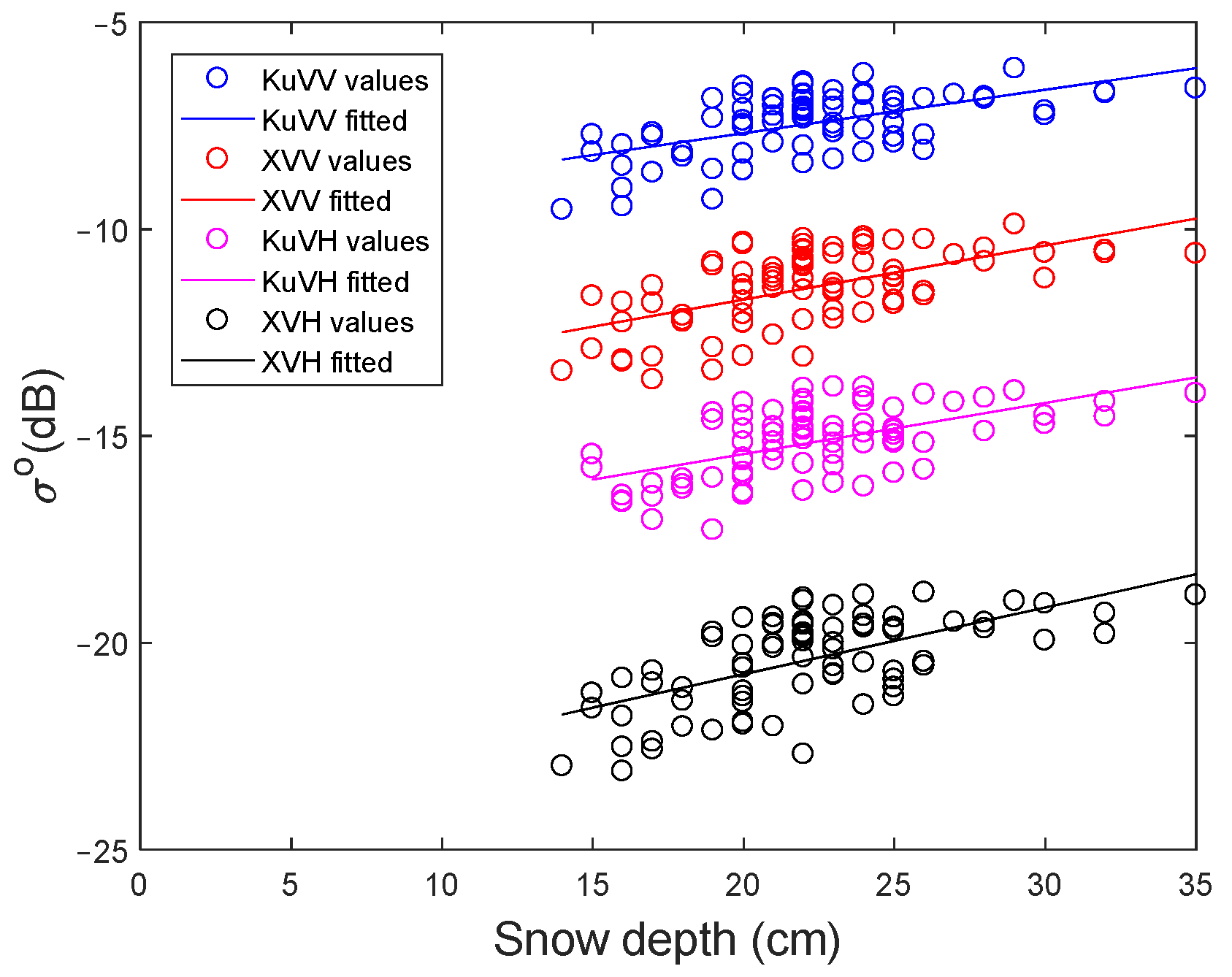
3.3. SnowSAR Data versus Snow Depth on Sea Ice

The in situ samples for the sea ice site covered only partly the SnowSAR acquisition; see Section 2.2.4. Only 20 samples out of 87 are within the SAR swath area. Among these samples, there were two points on smooth ice, one was located on a broken ice field, and two on ice ridges. The X- and Ku-band ${\mathsf{\sigma }}^{\mathrm{o}}$ as a function of snow depth for the sea ice site is presented in Figure 4. The channel ratios KuVV/KuVH and KuVV/XVV as a function of snow depth are shown in Figure 5. The statistics of the linear regression between the ${\mathsf{\sigma }}^{\mathrm{o}}$ data and snow depth are shown in

Table 6. Statistics of the linear regression between the SnowSAR backscattering coefficient and snow depth data for the sea ice site.

SnowSAR Band	Line Regression Statistics
	Slope Term	Offset	R2	p-Value
XVV	0.04	−15.3	0.02	0.545
XVH	0.05	−26.2	0.07	0.280
KuVV	0.09	−11.5	0.21	0.042
KuVH	0.05	−21.6	0.12	0.130
KuVV/KuVH	0.04	10.1	0.12	0.137
XVV/XVH	−0.01	10.8	0.10	0.692
KuVV/XVV	0.06	3.9	0.10	0.175
KuVH/XVH	0.01	4.6	0.00	0.881

.

At KuVV, the ${\mathsf{\sigma }}^{\mathrm{o}}$ was found to increase more in relation to snow depth (0.09 dB/cm) than in the case of XVV (0.04 dB/cm), KuVH (0.05 dB/cm) and XVH channels (0.05 dB/cm). However, at KuVV, R2 is only 0.21. Larger ${\mathsf{\sigma }}^{\mathrm{o}}$ values were observed for KuVV than for XVV; this frequency behavior is in line with previous studies, e.g., [28]. For XVH and KuVH, the ${\mathsf{\sigma }}^{\mathrm{o}}$ variation within snow depth was diminished by the SnowSAR noise floor. The highest sensitivity to snow depth within the channel ratios was found for KuVV/KuVH, but the R2 value was only 0.12.

The ${\mathsf{\sigma }}^{\mathrm{o}}$ data scatter was too large and the data amount too small for reliable conclusions about the behavior of either individual channels or the ratios as a function of the snow depth. The p-value of the linear regression was significant only for KuVV. In Figure 5b, KuVV/XVV slightly increases with increasing snow depth, which can be explained by a larger increase in snow volume scattering at the Ku- than at the X-band. The increase in KuVV/KuVH with increasing snow depth in Figure 5a could suggest a larger increase in single scattering in snow volume than of multiple scattering as a function of the snow depth. However, other variables such as snow density and grain size can also influence the ${\mathsf{\sigma }}^{\mathrm{o}}$ value. Unfortunately, our dataset did not allow us to study their effect on the ${\mathsf{\sigma }}^{\mathrm{o}}$.

It is worth noticing that $T_a$ during the SnowSAR image acquisition was −3.7 °C on the average. Some earlier studies indicate that if $T_a$ is warmer than −5 °C, there might be liquid water in the snow due to snow-melt onset, and the backscatter can be largely attenuated, e.g., [29]. Therefore, possible liquid water content in the snow may have decreased the ${\mathsf{\sigma }}^{\mathrm{o}}$ values.

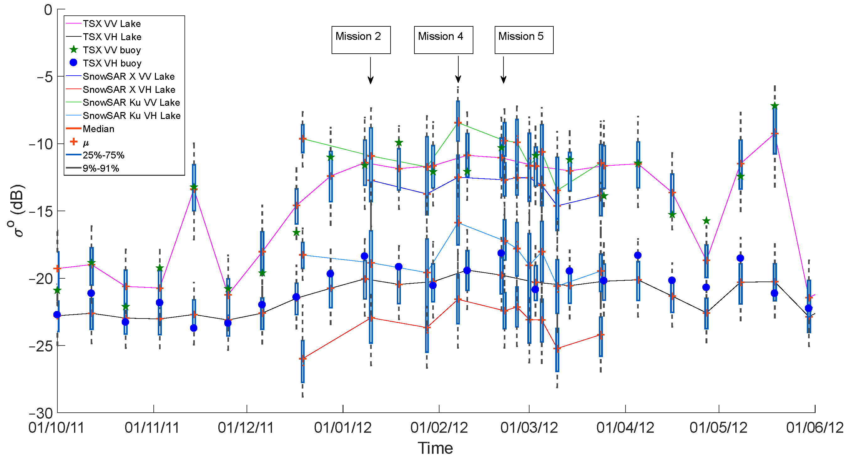
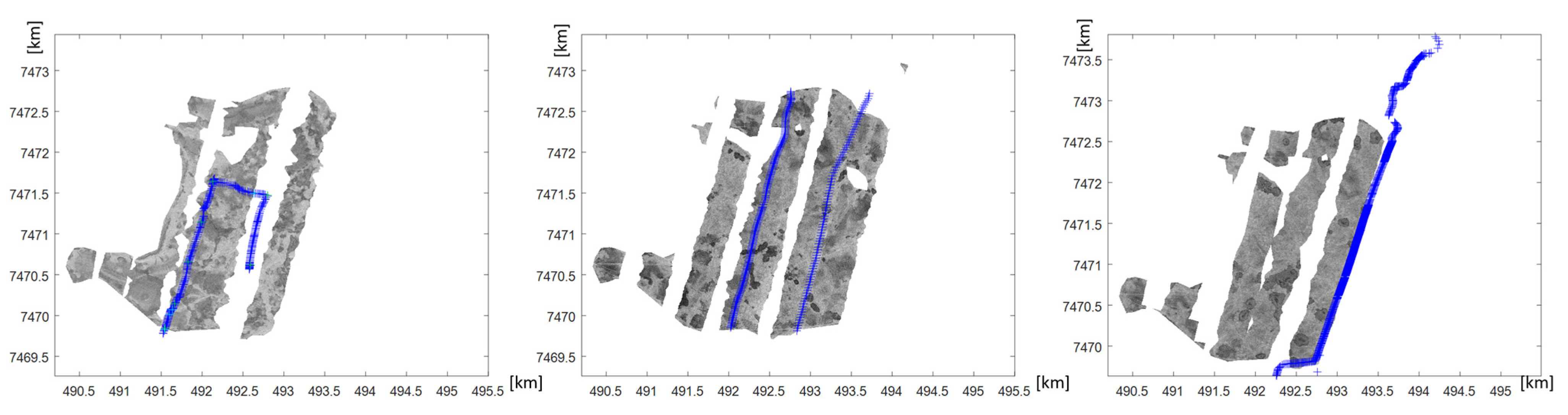
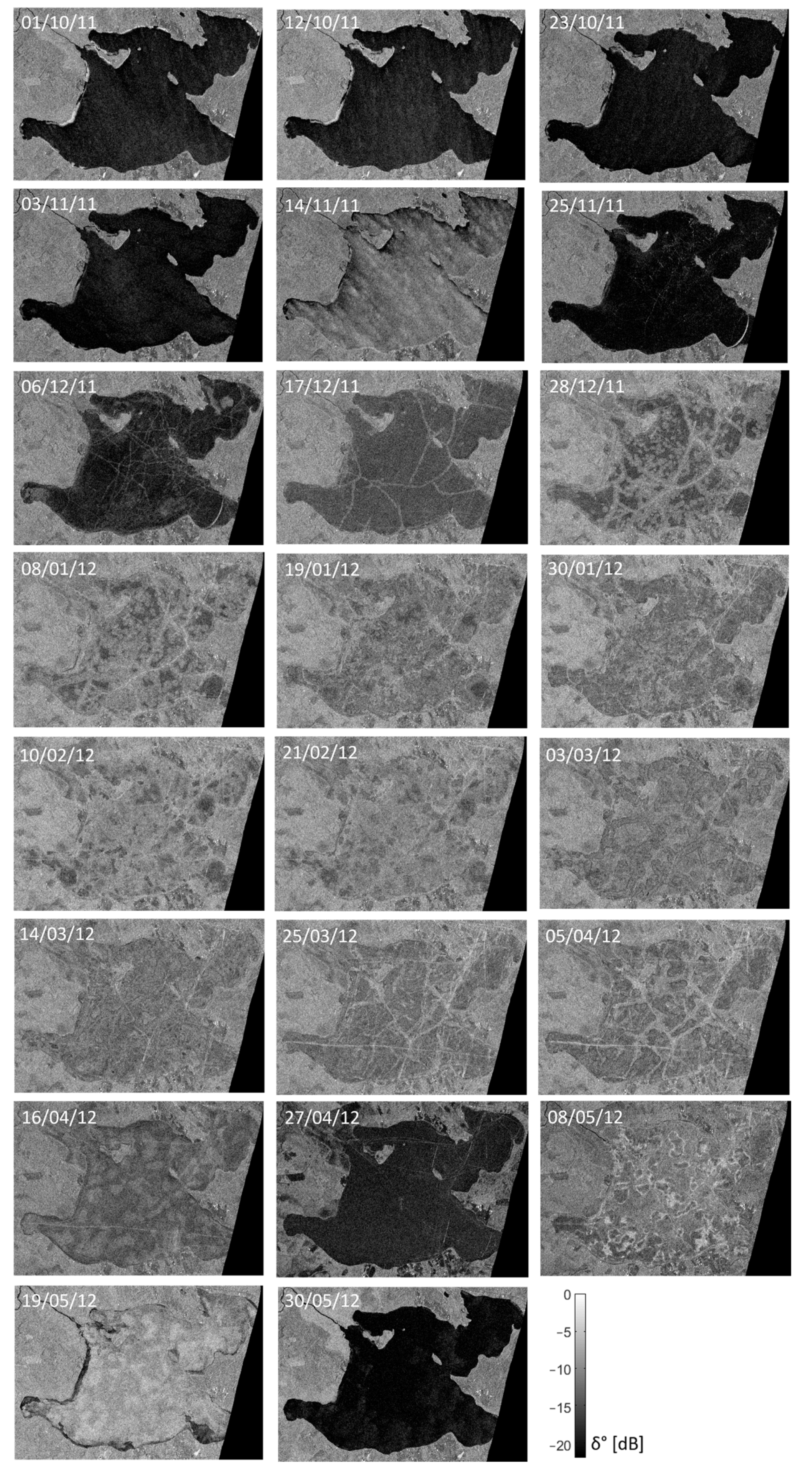
3.4. Analysis of TerraSAR-X Imagery Time Series on Lake Ice

3.4.1. Qualitative Analysis

TSX satellite StripMap imagery at VV- and VH-polarization over Lake Orajärvi, covering the time period from October 2011 to May 2012, was applied to analyze the variability of the X-band ${\mathsf{\sigma }}^{\mathrm{o}}$ signatures over time. In Figure 6, all TSX ${\mathsf{\sigma }}^{\mathrm{o}}$ images at VV-polarization are shown. In the images, distinct seasonal changes can be observed: after an initial low ${\mathsf{\sigma }}^{\mathrm{o}}$ typical for calm open water, a first sharp increase in the ${\mathsf{\sigma }}^{\mathrm{o}}$ can be observed on 14 November. At this time, ice was not yet formed on the lake, and the high ${\mathsf{\sigma }}^{\mathrm{o}}$ originated from waves caused by winds, as rough water surface areas have a high ${\mathsf{\sigma }}^{\mathrm{o}}$ [23]. The wind speed was 2.7–7.2 m/s (from light to moderate) and 5.4–13.8 m/s (from gentle to strong) in gusts.

The following TSX acquisition on 25 November shows again a low ${\mathsf{\sigma }}^{\mathrm{o}}$. During this acquisition, new, level congelation ice covered almost the entire lake, forming a highly specular surface with low backscatter characteristics. During the following acquisitions on 6, 17 and 28 December, the observed average ${\mathsf{\sigma }}^{\mathrm{o}}$ gradually increases, with the increasing of ${\mathsf{\sigma }}^{\mathrm{o}}$ concentrating around cracks and leads visible on the ice surface. Subsequent overflow of water on the ice surface and formation of a snow-ice layer causes these areas of increased ${\mathsf{\sigma }}^{\mathrm{o}}$ to gradually expand and eventually cover the whole area of the lake. During the cold winter period, metamorphism in ice and snow causes gradual spatial changes in the ${\mathsf{\sigma }}^{\mathrm{o}}$. In the spring acquisitions, on 16 and 27 April, the ${\mathsf{\sigma }}^{\mathrm{o}}$ drops as a result of warming weather and subsequent wetting of snow on top of the ice. The ${\mathsf{\sigma }}^{\mathrm{o}}$ increases again for acquisitions on 8 and 19 May, as lossy and highly specular wet snow is merged in the melting ice beneath [30]. In the acquisition on 19 May, shorelines of the lake can be seen in the SAR image to be already free of ice. After that, the ice melts quickly due to warm weather and the absence of snow on the ice, with the lake largely being ice-free in the last acquisition on 30 May.

The findings above suggest several possibilities to monitor the seasonal evolution of lake ice in Northern Europe using X-band SAR, including the onset and break-up of ice cover, wetting of the ice/snow surface, ice deformation, cracking, and slushing events. The high spatio-temporal variability of the ${\mathsf{\sigma }}^{\mathrm{o}}$ also explains some of the difficulties in associating snow conditions on lake ice directly with the ${\mathsf{\sigma }}^{\mathrm{o}}$ data. Previous studies of lake ice phenology have mostly used C-band SAR and QuickSAT Ku-band scatterometer data and have focused on the Arctic regions [31].

3.4.2. Time Series of TerraSAR-X Mean ${\sigma }^{\mathrm{o}}$ over Lake Ice

Figure 7 depicts the time series of the observed average TSX and SnowSAR ${\mathsf{\sigma }}^{\mathrm{o}}$ at VV- and VH-polarizations with boxplots over Lake Orajärvi. In addition, the mean ${\mathsf{\sigma }}^{\mathrm{o}}$ of TSX at the IMB location for VV and VH polarizations are shown. The closest TSX data in mission 2 are from one day before the SnowSAR flight and two days before the in situ data. For mission 4, the closest TSX data are from three days after the SnowSAR flight and one to two days after the in situ data. The closest TerraSAR data in mission 5 are from one day before the SnowSAR flight and the in situ data. Especially in Mission 4, there is a gap between the time of SnowSAR data and TSX data acquisition.

For TSX, the seasonal variation of the ${\mathsf{\sigma }}^{\mathrm{o}}$ is larger at the VV- than at the VH-polarization, but at VH a low signal-to-noise ratio has limited the variation. The noise equivalent TSX ${\mathsf{\sigma }}^{\mathrm{o}}$ is typically −22 dB [21]. The temporal TSX ${\mathsf{\sigma }}^{\mathrm{o}}$ trends at VV and VH are similar. For SnowSAR as well, the temporal ${\mathsf{\sigma }}^{\mathrm{o}}$ trends at VV and VH are quite similar, although at VH the ${\mathsf{\sigma }}^{\mathrm{o}}$ values for the Ku- and X-bands are more apart from each other. The trend of the Ku-band ${\mathsf{\sigma }}^{\mathrm{o}}$ is opposite to the X-band ${\mathsf{\sigma }}^{\mathrm{o}}$ from 19 December 2011–10 January 2012; 22–26 February 2012 and 1–5 March 2012 for both VV and VH. For the Ku-band, the ${\mathsf{\sigma }}^{\mathrm{o}}$ values are larger, and there is more variation in the time series than at the X-band. When the X-band ${\mathsf{\sigma }}^{\mathrm{o}}$ values for TSX and SnowSAR are compared, it can be seen that in VH there is more difference as the values are more apart from each other, although the trend is quite similar. There is a drop in the SnowSAR X-band time series on 10 March 2012 which is not that visible in the TSX ones. It should be noted that there are fewer data for SnowSAR.

The difference between the SnowSAR measurements in missions 2, 4 and 5 and the closest TerraSAR images were studied also by masking the SnowSAR image areas from the TerraSAR data. It did not have much effect, especially in mission 4. The use of that data would not give as good information about the temporal changes in the lake ice area, e.g., about the onset/offset of lake ice, as the areas close to the shores would be excluded.

The time series of the IMB snow depth data for Lake Orajärvi is shown in Figure 8a. In addition, $T_a$, rainfall intensity and snow depth from the closest AWS and the mean TSX ${\mathsf{\sigma }}^{\mathrm{o}}$ at the IMB location for both VV and VH polarizations are shown. Unfortunately, the IMB dataset does not cover the end of April with advanced ice-melting conditions. In Figure 8b, the IMB snow depth, ice thickness and measured temperature fields inside the snow and ice are presented.

The time series of the TSX ${\mathsf{\sigma }}^{\mathrm{o}}$ at the VV-polarization shows that the ${\mathsf{\sigma }}^{\mathrm{o}}$is low in October, when the lake is still free of ice. During open water conditions, the ${\mathsf{\sigma }}^{\mathrm{o}}$ rises occasionally due to waves, notably on 14 November, when high winds induced visible wave patterns in the SAR image (see Figure 6). In mid-November, $T_a$ drops below freezing, the lake ice starts forming and ${\mathsf{\sigma }}^{\mathrm{o}}$ increases. The AWS snow depth increases as well. The onset of snow accumulation in the AWS snow depth data in Figure 8a coincides with the peak in the ${\mathsf{\sigma }}^{\mathrm{o}}$ data series on 14 November.

During mid-winter, i.e., from December to March, the ${\mathsf{\sigma }}^{\mathrm{o}}$ is quite stable. Nevertheless, in two cases the ${\mathsf{\sigma }}^{\mathrm{o}}$ decreases although the snow depth increases. As time goes on, the ${\mathsf{\sigma }}^{\mathrm{o}}$ may increase due to recrystallization, i.e., reorganizing and growing of snow crystals [32].

The IMB snow depth varies between 9.7 cm and 30 cm, and the ${\mathsf{\sigma }}^{\mathrm{o}}$ at the VV-polarization during that period is between −13.9 dB and −9.9 dB. The ripple in the IMB snow depth data possibly indicates short-term variations caused by, for example, snowfall and melting events, or by accumulation or erosion of snow due to wind. In the IMB data, a sudden decrease in snow depth is visible in the end of February. A coinciding negative trend can be detected in both the VV- and VH-polarization ${\mathsf{\sigma }}^{\mathrm{o}}$values. For the VV-polarization ${\mathsf{\sigma }}^{\mathrm{o}}$, there is a ${\mathsf{\sigma }}^{\mathrm{o}}$ gradient of approximately −0.044 dB/day. For the IMB snow depth, there is a gradient of −1.6 cm/day. The sudden decrease in the IMB snow depth might be caused by the increase in the amount of snow-ice (i.e., snow converting to ice) as observed in the in situ measurements as well. The combined effect of extensive precipitation followed by high air humidity and cold $T_a$ could have caused the formation of snow-ice to take place. Even if there was no actual melting of snow, the snow metamorphoses may cause compaction of snow; in contrast, the AWS snow depth continues to increase because there is no formation of snow-ice on land. From late March to the beginning of April, after the AWS $T_a$ being above 0 °C, the ${\mathsf{\sigma }}^{\mathrm{o}}$ increases as $T_a$ decreases, snow refreezes and granular snow creates more volume scattering, and presumably also due to growing snow depth.

When the melting season starts, ${\mathsf{\sigma }}^{\mathrm{o}}$ starts to decrease as $T_a$ increases above 0 °C in April. The wetter the snow becomes, the lower the ${\mathsf{\sigma }}^{\mathrm{o}}$ values are. Later, ${\mathsf{\sigma }}^{\mathrm{o}}$ increases as the snow on ice melts completely. Unfortunately, there are no IMB data for the end of April to investigate reasons for the decrease in the ${\mathsf{\sigma }}^{\mathrm{o}}$. The onset of melting in the AWS snow depth data coincides with the drop in the VV-polarization ${\mathsf{\sigma }}^{\mathrm{o}}$ data series on 27 April. The time in the AWS snow depth data when all the snow has melted coincides with the peak in the VV-polarization ${\mathsf{\sigma }}^{\mathrm{o}}$ data series on 19 May.

In general, an increase in $T_a$ is seen as a decrease in the TSX ${\mathsf{\sigma }}^{\mathrm{o}}$, i.e., those are inversely correlated (R2 = 0.18, p = 0.05, when all TSX points are used; R2 = 0.54, p = 0.0001, when two points with the lowest and the highest $T_a$ values are excluded). In addition, the same kind of relation can be observed between $T_a$ and the IMB snow depth; the snow depth is higher during the cold periods. Warmer ice temperatures in Figure 8b, shown in dark red, are probably caused by a thicker snow layer [33] or generally warmer $T_a$ at that moment.

Next, we investigate the influence of the temperatures inside the snow volume on the ${\mathsf{\sigma }}^{\mathrm{o}}$. Layers of different temperatures within the snowpack were investigated more closely. As an example, the layer in snow having a temperature between −1.75 °C and −2.5 °C at 18:00 LT on the days of the TSX image acquisition is shown separately as a blue curve in the temperature field in Figure 8b. It was found to be the most consistent temperature interval with the time series of the TSX ${\mathsf{\sigma }}^{\mathrm{o}}$ data. After March, this consistency does not apply. Instead, the layer with the temperature between −5 °C and −10 °C is after the middle of March more valid.

It can be seen in Figure 8a,b that the days before mission 4 were very cold (−38.8 °C at the coldest on 5 February 2012) and several days without snowing until fresh snow fell just before the SnowSAR acquisition. The lake ice had also become thicker. In mission 5 as well, it was snowing before the SnowSAR acquisition, but $T_a$ had not been as cold as in mission 4. In the case of mission 2, snowfall was not detected between the SnowSAR acquisition and the collection of in situ data.

4. Discussion

4.1. Previous Studies

In the following, we discuss previous studies on snow depth and snow water equivalent (SWE) estimation on sea ice and lake ice using the MR and SAR data. We also discuss how sea ice and lake ice properties and the ${\mathsf{\sigma }}^{\mathrm{o}}$ are typically related.

Operational methods for snow depth (or SWE) estimation over sea ice with the MR data have been developed in many studies, e.g., [12,34,35]. Currently, the MR-based snow depth data are accurate only over smooth first-year ice (FYI) [7,34,36,37]. Over deformed FYI or multiyear ice (MYI), snow depth is substantially underestimated [37]. The operational algorithms are typically based on the 19 GHz (K-band) and 37 GHz (Ka-band) brightness temperature ($T_B$) data and snow $T_B$ signature difference between these two frequencies. Snow depth estimation accuracy is also in general degraded by a mixture of various ice types typically present within large MR footprints. Snow depth on sea ice has also been investigated by using numerical one-dimensional snow and sea ice thermodynamic models, e.g., [38,39]. Recently, snow depth on sea ice has been estimated also by using satellite altimetry [40,41,42], for example, by using dual-frequency radar freeboards or coincident satellite radar and lidar altimetry. In the coming Copernicus Polar Ice and Snow topography Altimeter (CRISTAL) high-priority mission, a dual-frequency satellite altimeter will provide information about snow depth on sea ice and will also help to discriminate between the ice and snow interfaces [43]. As for sea ice, for lake ice many studies on snow and ice properties and their temporal changes have also been conducted using thermodynamic models, e.g., [19,44], and a Snow Microwave Radiative Transfer (SMRT) model [45]. Lake ice thickness has been studied using the satellite altimeter, moderate resolution imaging spectroradiometer (MODIS) and MR data, and in addition phenology studies have been conducted [14,46,47].

Products for the snow depth over Arctic sea ice retrieved from altimeter and MR satellite measurements as well as from reanalysis have been compared recently [48]. They highlighted the need for more targeted Arctic surveys with different spatial and temporal scales to be able to make a more systematic comparison of airborne, in situ and satellite-based observations. In a recent study, CryoSat-2 altimeter measurements have been combined with passive microwave (AMSR) and infrared (AVHRR) measurements to obtain snow depth on sea ice [31].

In order to obtain information of snow depth at fine spatial scales (~0.1–1 km), the use of SAR data, which have much better spatial resolution than MRs, has been investigated in some case studies, e.g., [49,50,51]. These have not yet resulted in any operational applications. So far, studies have been conducted mainly with C-band SAR sensors due to the availability of a large amount of SAR imagery. However, theoretical investigations indicate that the effect of snow cover on sea ice to radar backscattering at the X- and Ku-band can be more pronounced than at the C-band [28,52,53,54].

There are several factors that influence the ${\mathsf{\sigma }}^{\mathrm{o}}$ of a target: both the parameters of the SAR sensor and the properties of the target itself. Examples of the former are wavelength (frequency), polarization, incidence angle, and resolution and, of the latter, surface roughness (compared to the SAR wavelength), volume fraction, size, and shape of the scatterers in the media, and relative permittivities of the scatterers and the host media. In the case of snow-covered lake and sea ice, snow depth, snow density, snow microstructure (e.g., crystal size), amount of liquid water in the snowpack and surface roughness contribute to the measured ${\mathsf{\sigma }}^{\mathrm{o}}$. These snow properties vary spatially and temporally as a result of snow transport by wind, melt–refreeze events, and snow deposition and metamorphism.

Different backscattering sources contributing to the measured ${\mathsf{\sigma }}^{\mathrm{o}}$ for sea ice and lake ice are shown in Figure 9. These include surface scattering at the air–snow, snow–ice and ice–water interfaces, as well as scattering in the ice and snow volumes [23,24]. Typically, dry snow cover on ice increases the ${\mathsf{\sigma }}^{\mathrm{o}}$ compared to the case of bare ice through the increased backscattering in the snow volume [24,55]. For sea ice, the total ${\mathsf{\sigma }}^{\mathrm{o}}$ typically consists of surface scattering from the snow surface, volume scattering from the snow layer, surface scattering from the ice surface and scattering from the air bubbles and brine pockets in the ice medium. For lake ice, there is more volume scattering from the lower layers of the ice; surface scattering from internal layers in the ice, scattering from the ice–water surface and double-bounce scattering from the bottom bubbled ice layer are included as well [56,57]. In recent studies, the scattering caused by the roughness of the ice–water interface has been found to be the primary contribution to the total scattering over lake ice and not the double bounce from air bubbles, as has been assumed previously [46,58]. In the case of wet snow, the high dielectric contrast between air and wet snow causes scattering from the snow surface to become a dominant factor [24]. In the case of rough ice, the effect of dry snow cover can be negligible, with the ice surface scattering being a dominating factor, especially in lower frequencies, e.g., at the C-band [24,28].

An investigation using C-band SAR indicated that changes in the dielectric properties of snow cover due to an air temperature change are detectable in the ${\mathsf{\sigma }}^{\mathrm{o}}$ for smooth thick landfast FYI [49]. This allowed to detect SWE changes using SAR image pairs, one acquired in cold (~−26 °C) and one in moderately cold (~−14 °C) conditions. Snow cover affects the temperature of the upper surface of the ice, which affects the brine volume, dielectric properties and scattering characteristics within the snow volume [49]. In higher temperatures, the snow grains become brine-wetted and produce volume scattering.

It has been found that even a thin snow cover (2 cm) increases the ${\mathsf{\sigma }}^{\mathrm{o}}$ at an oblique incidence angle at the C- and Ku-bands [55]. However, increasing dry snow depth did not further influence the ${\mathsf{\sigma }}^{\mathrm{o}}$ [55]. On the contrary to cold conditions (−7.9 °C), no relationship between various radar polarimetric parameters and snow depth was found under warmer conditions (−0.4 °C) [51]. The results suggested that snow depth estimation based on snow thermodynamics at warm conditions is not possible, whereas during cold winter conditions (<−10 °C), snow depth could be retrieved from SAR data. In general, for sea ice ${\mathsf{\sigma }}^{\mathrm{o}}$ at the C-band, volume or mixed scattering components increase with increasing snow depth, most likely due to brine-wetted snow layers at the ice-snow interface [51].

Investigations using higher frequencies, such as X-band, show that the effect of snow cover on the ${\mathsf{\sigma }}^{\mathrm{o}}$ is large, especially in the case of FYI [28]. For lake ice, the Ku-band ${\mathsf{\sigma }}^{\mathrm{o}}$, measured with ground-based scatterometers, has been found to be sensitive to the snowpack, whereas the X-band ${\mathsf{\sigma }}^{\mathrm{o}}$ was found to be largely insensitive [59]. Based on the scatterometer measurements, as the wavelength is shorter at the Ku-band (17.4 mm) compared to the X-band (31 mm), the interaction with initial tubular bubble formation (see Figure 9) close to the ice–water interface and with grains within the snowpack above the ice may be increased [60].

SAR imagery has been also used for lake ice classification (open water and various ice types, ice break-up) and to detect floating and bedfast lake ice regimes in the Arctic, e.g., [61,62,63,64]. In addition, using polarimetric decomposition in order to understand scattering processes in freshwater ice has been investigated recently [65].

Finally, a comprehensive review of the remote sensing of lake and river ice presented nearly ten years ago by Duguay et al. [31] stated that, to their knowledge, no operational method has yet been developed for estimating snow depth or SWE on lake ice. To our knowledge, this is still the case.

4.2. Discussion of This Study

Backscattering from snow-covered lake or sea ice is a complex function of various snow and ice parameters (e.g., snow depth and snow grain size), and is composed of various surface and volume scattering components, whose relative magnitudes depend on the snow and ice properties. These complexities add a challenge to deriving relations between the measured ${\mathsf{\sigma }}^{\mathrm{o}}$ and bulk snow properties such as snow depth or SWE, which would be needed to enhance the accuracy of present lake and sea ice mass balance estimates. However, as sufficient information on ice and snow structural properties is typically unavailable at the accuracy required to properly set up retrieval algorithms based on complex simulation schemes (see, e.g., [59]), analyzing direct relations of ${\mathsf{\sigma }}^{\mathrm{o}}$ and bulk snow properties remain appealing, as such analysis gives indications of the usability of the SAR data for practical operational retrieval schemes.

For lake ice, we showed that the X-band VH-polarized ${\mathsf{\sigma }}^{\mathrm{o}}$ and the Ku-band VV/VH- or KuVH/XVH ratio exhibited the highest direct sensitivity to the snow depth; however, statistically significant relations appeared only for one of the investigated missions with co-incident SAR and in situ information available. For sea ice, the highest sensitivity to the snow depth was found from the Ku-band VV-polarized ${\mathsf{\sigma }}^{\mathrm{o}}$ and the Ku-band VV/VH-ratio. However, in the linear regression analysis the observed coefficients of determination were found to be weak or moderate, indicating that snow depth alone was insufficient to explain the observed patterns in the ${\mathsf{\sigma }}^{\mathrm{o}}$ data, and other factors such as variations in ice surface roughness, ice and air inclusions, and snow microstructure carry a large effect on the ${\mathsf{\sigma }}^{\mathrm{o}}$ at both X- and Ku-bands. This is in line with similar studies using the SnowSAR data over land [66], where the overall influence of the bulk snow properties (SWE and snow depth) on ${\mathsf{\sigma }}^{\mathrm{o}}$ was found to be largely masked by variations in the snow effective microstructure and ground surface roughness. The observed weak relations indicate that in practice, the relative benefit of the X- and Ku-band SAR in deriving information on the bulk snow properties over ice is limited. However, in particular for the case of the sea ice site here, the range in snow depth was small; more significant snow depth variations could reveal stronger relations in the ${\mathsf{\sigma }}^{\mathrm{o}}$. In addition, $T_a$ during the SnowSAR acquisition over the sea ice site might have been too warm (moisture in snow) and caused attenuation to the received backscattering signal, although during the in situ measurements, the snow was qualitatively observed to be dry. Nonlinear fitting was also tried, and multiple factors could be considered, although in this article the focus was on investigating if it would be possible to estimate snow depth by using only linear fitting to the backscatter data. Thus, multiple regressions are not used in the data analyses. Further, using multiple snow parameters, like snow density and snow grain size, in the regression would not allow estimating any single snow parameter from the backscatter data. Furthermore, only limited data on other snow parameters than depth were available; a snow pit with detailed stratigraphy, for example, was typically available from one location only.

Qualitative analysis of the TSX imagery time series over Lake Orajärvi covering a whole winter period gave indications of the complexity of factors affecting the ${\mathsf{\sigma }}^{\mathrm{o}}$ for snow-covered lake ice. Metamorphism processes in both the snow and underlying ice due to weather effects and physical stresses result in a highly variable temporal ${\mathsf{\sigma }}^{\mathrm{o}}$ response. However, our results confirm X-band SAR to be a useful tool in monitoring events such as onset and break-up of ice, slushing events on the ice surface, wetting of the ice/snow during the spring. Previous studies of lake ice phenology have mostly used C-band SAR and QuickSAT Ku-band scatterometer data and focused on the Arctic regions [31]. Together with ice type classification based on C-band SAR observations (e.g., [67]), X-band SAR observations may find further operational use in ice charting of freshwater lakes, with implications for ice safety management.

The main reason for the better result for mission 4 than for other missions could be the scale of snow depths in the dataset; that is, the standard deviation of ice thickness was smaller than in mission 2, suggesting that the ice could have been more like level ice. The ice was thicker in mission 4 than in mission 2, and before SnowSAR data acquisition in mission 4 there had been cold air temperatures and it was snowing fresh snow just before the SnowSAR data acquisition.

The presented analysis was limited to a single lake and sea ice campaign; the work should be continued by investigating more comprehensive datasets representing diverse sea and lake ice conditions. More comprehensive measurements of variables such as ice surface roughness, air bubble inclusions in ice, snow density, temperature, grain size, SWE, and moisture would be required in order to make more reliable conclusions of the behavior of the ${\mathsf{\sigma }}^{\mathrm{o}}$ vs. snow depth on ice. In the future, it would be interesting to investigate the capability to estimate the snow depth from the SAR data with combinations of other frequencies such as Ka-band, as well as for different ice types. In addition, theoretical ${\mathsf{\sigma }}^{\mathrm{o}}$ models, and possibly polarimetric X- and Ku-band SAR data could be used to reveal radar signal characteristics and relations to snow properties which were not analysed here.

5. Conclusions

We investigated the relationship between ${\mathsf{\sigma }}^{\mathrm{o}}$ measured using an airborne SAR instrument (SnowSAR) operating at the X- and Ku-bands, and the snow depth measured in situ, over lake ice in Lake Orajärvi in northern Finland and sea ice in the Bay of Bothnia of the Baltic Sea. To our knowledge, this study is the first comprehensive survey of airborne SAR ${\mathsf{\sigma }}^{\mathrm{o}}$ signatures at the X- and Ku-bands over both lake and sea ice. Airborne SAR surveys at these frequencies are necessary to increase our understanding of the complex radar signatures of snow-covered ice. Specifically, this study is one of the first ones analyzing spatially distributed signatures at the Ku-band, which due to the short wavelength is sensitive to properties of dry snowpack through volume scattering [59].

For lake ice, for mission 4, we showed that the best correlations between the ${\mathsf{\sigma }}^{\mathrm{o}}$ and snow depth were found for the X-band VH-polarized ${\mathsf{\sigma }}^{\mathrm{o}}$ and the ${\mathsf{\sigma }}^{\mathrm{o}}$ polarization ratio of KuVV/KuVH or KuVH/XVH. A statistically significant increase in backscatter with increasing snow depth was found for all individual channels; however, the calculated coefficient of determination for the linear regression was weak or moderate (0.2–0.4). However, these relations seem incidental, as they appeared for only one of the investigated SnowSAR missions. For several subsequent and preceding missions, statistically significant relations between backscatter and snow depth could not be identified. For some cases, the number of data samples was limited, and the distribution in snow depth too small to provide a reliable analysis. However, the major reason for the loss of sensitivity may be due to changes in the subnivean ice backscattering conditions, which change notably both spatially and temporally, and possibly supersede any variability induced by variations in volume scattering from snow depth. This is supported by analysis of the TerraSAR-X data over the same lake, which show notable spatio-temporal variability of the X-band backscattering signal, which qualitatively can be attributed to, e.g., cracks and slushing of water on the ice-snow interface, causing visible variations in backscattering conditions.

For sea ice, the small amount of coincident SnowSAR and in situ data limited the reliability of analyzed relationships between the SnowSAR ${\mathsf{\sigma }}^{\mathrm{o}}$ and the in situ snow depth. However, based on the limited data, the Ku-band VV-polarization ${\mathsf{\sigma }}^{\mathrm{o}}$ and the polarization ratio KuVV/KuVH showed the highest sensitivity to the snow depth. As for lake ice, the Ku-band ${\mathsf{\sigma }}^{\mathrm{o}}$ increased with the increasing snow depth, indicating an increase in snow volume scattering. However, the X-band signatures over sea ice revealed less sensitivity than over lake ice. Overall, the observed relations were weaker than for lake ice (max R2 was 0.21). The different results for lake and sea ice are possibly due to different dataset sizes, different ranges in snow depth or differences in stratigraphy and properties in snow cover over lake and sea ice, and differences in ice surface roughness and ice medium properties (e.g., fresh lake ice vs. slightly saline sea ice).

TSX SAR data were used along with the Ice Mass Balance Buoy (IMB) data from Lake Orajärvi to compare the evolution of snow depth and ${\mathsf{\sigma }}^{\mathrm{o}}$. As expected, seasonal variation of the snow depth on lake ice was observed. The analysis of the TSX ${\mathsf{\sigma }}^{\mathrm{o}}$ time series gives indications of the complexity of factors affecting backscattering over snow-covered ice. However, X-band SAR can be a useful tool to monitor for example the onset and break-up of ice, slushing events on the ice surface or wetting of the ice/snow in spring.

In general, the results indicate that obtaining reliable estimates of snow depth over lake and sea ice would be challenging by using only X- and Ku-band backscattering information. To better tackle this challenge, possibly applying some other data, e.g., altimeter data, could improve the estimation of snow depth.

References

1. Maykut, G.A. Energy Exchange over Young Sea Ice in the Central Arctic. J. Geophys. Res. Oceans 1978, 83, 3646–3658. [Google Scholar] [CrossRef]
2. Leppäranta, M. A Growth Model for Black Ice, Snow Ice and Snow Thickness in Subarctic Basins. Hydrol. Res. 1983, 14, 59–70. [Google Scholar] [CrossRef]
3. Fichefet, T.; Maqueda, M.A.M. Modelling the Influence of Snow Accumulation and Snow-Ice Formation on the Seasonal Cycle of the Antarctic Sea-Ice Cover. Clim. Dyn. 1999, 15, 251–268. [Google Scholar] [CrossRef]
4. Giles, K.A.; Laxon, S.W.; Wingham, D.J.; Wallis, D.W.; Krabill, W.B.; Leuschen, C.J.; McAdoo, D.; Manizade, S.S.; Raney, R.K. Combined Airborne Laser and Radar Altimeter Measurements over the Fram Strait in May 2002. Remote Sens. Environ. 2007, 111, 182–194. [Google Scholar] [CrossRef]
5. Shen, X.; Ke, C.-Q.; Wang, Q.; Zhang, J.; Shi, L.; Zhang, X. Assessment of Arctic Sea Ice Thickness Estimates From ICESat-2 Using IceBird Airborne Measurements. IEEE Trans. Geosci. Remote Sens. 2021, 59, 3764–3775. [Google Scholar] [CrossRef]
6. Kurtz, N.T.; Farrell, S.L. Large-Scale Surveys of Snow Depth on Arctic Sea Ice from Operation IceBridge. Geophys. Res. Lett. 2011, 38, L20505:1–L20505:5. [Google Scholar] [CrossRef]
7. Brucker, L.; Markus, T. Arctic-Scale Assessment of Satellite Passive Microwave-Derived Snow Depth on Sea Ice Using Operation IceBridge Airborne Data. J. Geophys. Res. Oceans 2013, 118, 2892–2905. [Google Scholar] [CrossRef]
8. Yan, J.-B.; Gomez-Garcia Alvestegui, D.; McDaniel, J.W.; Li, Y.; Gogineni, S.; Rodriguez-Morales, F.; Brozena, J.; Leuschen, C.J. Ultrawideband FMCW Radar for Airborne Measurements of Snow Over Sea Ice and Land. IEEE Trans. Geosci. Remote Sens. 2017, 55, 834–843. [Google Scholar] [CrossRef]
9. Rodriguez-Morales, F.; Leuschen, C.; Carabajal, C.L.; Paden, J.; Wolf, J.A.; Garrison, S.; McDaniel, J.W. An Improved UWB Microwave Radar for Very Long-Range Measurements of Snow Cover. IEEE Trans. Instrum. Meas. 2020, 69, 7761–7772. [Google Scholar] [CrossRef]
10. Jenssen, R.O.R.; Eckerstorfer, M.; Jacobsen, S. Drone-Mounted Ultrawideband Radar for Retrieval of Snowpack Properties. IEEE Trans. Instrum. Meas. 2020, 69, 221–230. [Google Scholar] [CrossRef]
11. Murfitt, J.; Duguay, C.R. 50 Years of Lake Ice Research from Active Microwave Remote Sensing: Progress and Prospects. Remote Sens. Environ. 2021, 264, 112616. [Google Scholar] [CrossRef]
12. Markus, T.; Cavalieri, D.J. Snow Depth Distribution Over Sea Ice in the Southern Ocean from Satellite Passive Microwave Data. In Antarctic Research Series; Jeffries, M.O., Ed.; American Geophysical Union: Washington, DC, USA, 2013; pp. 19–39. ISBN 978-1-118-66824-5. [Google Scholar]
13. Hallikainen, M.; Winebrenner, D.P. The Physical Basis for Sea Ice Remote Sensing. In Geophysical Monograph Series; Carsey, F.D., Ed.; American Geophysical Union: Washington, DC, USA, 1992; Volume 68, pp. 29–46. ISBN 978-0-87590-033-9. [Google Scholar]
14. Du, J.; Kimball, J.S.; Duguay, C.; Kim, Y.; Watts, J.D. Satellite Microwave Assessment of Northern Hemisphere Lake Ice Phenology from 2002 to 2015. Cryosphere 2017, 11, 47–63. [Google Scholar] [CrossRef]
15. Rott, H.; Yueh, S.H.; Cline, D.W.; Duguay, C.; Essery, R.; Haas, C.; Hélière, F.; Kern, M.; Macelloni, G.; Malnes, E.; et al. Cold Regions Hydrology High-Resolution Observatory for Snow and Cold Land Processes. Proc. IEEE 2010, 98, 752–765. [Google Scholar] [CrossRef]
16. Trampuz, C.; Coccia, A.; Imbembo, E. Technical Assistance for the Development and Deployment of an X- and Ku- Band MiniSAR Airborne System; Metasensing, Final Report, Contract 4000101697/10/NL/FF/ef. 2011. Available online: https://earth.esa.int/eogateway/documents/20142/37627/SnowSAR-FinalReport_DataSet_Desc.pdf (accessed on 8 January 2024).
17. Palosuo, E.; Leppäranta, M.; Seinä, A. Formation, Thickness and Stability of Fast Ice along the Finnish Coast; Winter Navig. Res. Board: Helsinki, Finland, 1982; Available online: https://www.traficom.fi/sites/default/files/12795-Report_No_36_FORMATION%2C_THICKNESS_AND_STABILITY_OF_FAST_ICE_ALONG_THE_FINNISH_COAST.pdf (accessed on 8 January 2024).
18. Hallikainen, M. Microwave Remote Sensing of Low-Salinity Sea Ice. In Geophysical Monograph Series; Carsey, F.D., Ed.; American Geophysical Union: Washington, DC, USA, 1992; Volume 68, pp. 361–373. ISBN 978-0-87590-033-9. [Google Scholar]
19. Cheng, B.; Vihma, T.; Rontu, L.; Kontu, A.; Pour, H.K.; Duguay, C.; Pulliainen, J. Evolution of Snow and Ice Temperature, Thickness and Energy Balance in Lake Orajärvi, Northern Finland. Tellus Dyn. Meteorol. Oceanogr. 2014, 66, 21564. [Google Scholar] [CrossRef]
20. Di Leo, D.; Coccia, A.; Meta, A. Technical Assistance for the Development and Deployment of an X- and Ku-Band MiniSAR Airborne System (SnowSAR). Analysis and Comments on SnowSAR Datasets, Final Report, Contract 4000101697/10/NL/FF/ef. 2016. Available online: https://earth.esa.int/eogateway/documents/20142/37627/SnowSAR-Final-Report-MS-EST-SNW-03-TCN-258.pdf (accessed on 8 January 2024).
21. Schwerdt, M.; Schmidt, K.; Klenk, P.; Tous Ramon, N.; Rudolf, D.; Raab, S.; Weidenhaupt, K.; Reimann, J.; Zink, M. Radiometric Performance of the TerraSAR-X Mission over More Than Ten Years of Operation. Remote Sens. 2018, 10, 754. [Google Scholar] [CrossRef]
22. Lemmetyinen, J.; Kontu, A.; Pulliainen, J.; Mäkynen, M. Synergy of CoReH2O SAR and Microwave Radiometry Data to Retrieve Snow and Ice Parameters—Task 1 Report; ESA Study, Contract 22829/09/NL/JC; European Space Agency: Paris, France, 2013. [Google Scholar]
23. Ulaby, F.T.; Moore, R.K.; Fung, A.K. Microwave Remote Sensing. 2: Radar Remote Sensing and Surface Scattering and Emission Theory; Remote Sensing; Addison-Wesley: Reading, MA, USA, 1982; ISBN 978-0-201-10760-9. [Google Scholar]
24. Fung, A.K. Microwave Scattering and Emission Models and Their Applications; The Artech House Remote Sensing Library; Artech House: Boston, MA, USA, 1994; ISBN 978-0-89006-523-5. [Google Scholar]
25. Makynen, M.; Cheng, B.; Simila, M.; Vihma, T.; Hallikainen, M. Interpretation of C-Band SAR Backscattering Coefficient Time Series for the Baltic Sea Landfast Sea Ice Using a 1-D Thermodynamic Snow/Ice Model. In Proceedings of the 2007 IEEE International Geoscience and Remote Sensing Symposium, Barcelona, Spain, 23–28 July 2007; pp. 3983–3986. [Google Scholar]
26. Paterson, W.S.B. The Physics of Glaciers, 3rd ed.; Pergamon: Oxford, UK; Tarrytown, NY, USA, 1994; ISBN 978-0-08-037945-6. [Google Scholar]
27. Kontu, A. Effect of Snow Microstructure and Subnivean Water Bodies on Microwave Radiometry of Seasonal Snow. Doctoral Thesis, Aalto University, Espoo, Finland, 2018. [Google Scholar]
28. Kim, Y.-S.; Onstott, R.; Moore, R. Effect of a Snow Cover on Microwave Backscatter from Sea Ice. IEEE J. Ocean. Eng. 1984, 9, 383–388. [Google Scholar] [CrossRef]
29. Howell, S.E.L.; Brown, L.C.; Kang, K.-K.; Duguay, C.R. Variability in Ice Phenology on Great Bear Lake and Great Slave Lake, Northwest Territories, Canada, from SeaWinds/QuikSCAT: 2000–2006. Remote Sens. Environ. 2009, 113, 816–834. [Google Scholar] [CrossRef]
30. Shokr, M.; Sinha, N. Sea Ice: Physics and Remote Sensing; John Wiley & Sons: Hoboken, NJ, USA, 2015; ISBN 978-1-119-02789-8. [Google Scholar]
31. Duguay, C.R.; Bernier, M.; Gauthier, Y.; Kouraev, A. Remote Sensing of Lake and River Ice. In Remote Sensing of the Cryosphere; Tedesco, M., Ed.; John Wiley & Sons, Ltd.: Chichester, UK, 2014; pp. 273–306. ISBN 978-1-118-36890-9. [Google Scholar]
32. Leinss, S.; Parrella, G.; Hajnsek, I. Snow Height Determination by Polarimetric Phase Differences in X-Band SAR Data. IEEE J. Sel. Top. Appl. Earth Obs. Remote Sens. 2014, 7, 3794–3810. [Google Scholar] [CrossRef]
33. Cai, Y.; Ke, C.-Q.; Duan, Z. Monitoring Ice Variations in Qinghai Lake from 1979 to 2016 Using Passive Microwave Remote Sensing Data. Sci. Total Environ. 2017, 607–608, 120–131. [Google Scholar] [CrossRef]
34. Comiso, J.C.; Cavalieri, D.J.; Markus, T. Sea Ice Concentration, Ice Temperature, and Snow Depth Using AMSR-E Data. IEEE Trans. Geosci. Remote Sens. 2003, 41, 243–252. [Google Scholar] [CrossRef]
35. Maaß, N.; Kaleschke, L.; Tian-Kunze, X.; Drusch, M. Snow Thickness Retrieval over Thick Arctic Sea Ice Using SMOS Satellite Data. Cryosphere 2013, 7, 1971–1989. [Google Scholar] [CrossRef]
36. Markus, T.; Cavalieri, D.J.; Gasiewski, A.J.; Klein, M.; Maslanik, J.A.; Powell, D.C.; Stankov, B.B.; Stroeve, J.C.; Sturm, M. Microwave Signatures of Snow on Sea Ice: Observations. IEEE Trans. Geosci. Remote Sens. 2006, 44, 3081–3090. [Google Scholar] [CrossRef]
37. Kern, S.; Ozsoy-Cicek, B.; Willmes, S.; Nicolaus, M.; Haas, C.; Ackley, S. An Intercomparison between AMSR-E Snow-Depth and Satellite C- and Ku-Band Radar Backscatter Data for Antarctic Sea Ice. Ann. Glaciol. 2011, 52, 279–290. [Google Scholar] [CrossRef]
38. Merkouriadi, I.; Cheng, B.; Graham, R.M.; Rösel, A.; Granskog, M.A. Critical Role of Snow on Sea Ice Growth in the Atlantic Sector of the Arctic Ocean. Geophys. Res. Lett. 2017, 44, 10479–10485. [Google Scholar] [CrossRef]
39. Cheng, B.; Zhang, Z.; Vihma, T.; Johansson, M.; Bian, L.; Li, Z.; Wu, H. Model Experiments on Snow and Ice Thermodynamics in the Arctic Ocean with CHINARE 2003 Data. J. Geophys. Res. 2008, 113, C09020. [Google Scholar] [CrossRef]
40. Kern, S.; Ozsoy-Çiçek, B. Satellite Remote Sensing of Snow Depth on Antarctic Sea Ice: An Inter-Comparison of Two Empirical Approaches. Remote Sens. 2016, 8, 450. [Google Scholar] [CrossRef]
41. Lawrence, I.R.; Tsamados, M.C.; Stroeve, J.C.; Armitage, T.W.K.; Ridout, A.L. Estimating Snow Depth over Arctic Sea Ice from Calibrated Dual-Frequency Radar Freeboards. Cryosphere 2018, 12, 3551–3564. [Google Scholar] [CrossRef]
42. Kwok, R.; Kacimi, S.; Webster, M.A.; Kurtz, N.T.; Petty, A.A. Arctic Snow Depth and Sea Ice Thickness from ICESat-2 and CryoSat-2 Freeboards: A First Examination. J. Geophys. Res. Oceans 2020, 125, e2019JC016008. [Google Scholar] [CrossRef]
43. Kern, M.; Cullen, R.; Berruti, B.; Bouffard, J.; Casal, T.; Drinkwater, M.R.; Gabriele, A.; Lecuyot, A.; Ludwig, M.; Midthassel, R.; et al. The Copernicus Polar Ice and Snow Topography Altimeter (CRISTAL) High-Priority Candidate Mission. Cryosphere 2020, 14, 2235–2251. [Google Scholar] [CrossRef]
44. Wei, L.; Deng, X.; Cheng, B.; Vihma, T.; Hannula, H.-R.; Qin, T.; Pulliainen, J. The Impact of Meteorological Conditions on Snow and Ice Thickness in an Arctic Lake. Tellus Dyn. Meteorol. Oceanogr. 2016, 68, 31590. [Google Scholar] [CrossRef]
45. Murfitt, J.; Duguay, C.R.; Picard, G.; Gunn, G.E. Investigating the Effect of Lake Ice Properties on Multifrequency Backscatter Using the Snow Microwave Radiative Transfer Model. IEEE Trans. Geosci. Remote Sens. 2022, 60, 1–23. [Google Scholar] [CrossRef]
46. Beckers, J.F.; Alec Casey, J.; Haas, C. Retrievals of Lake Ice Thickness From Great Slave Lake and Great Bear Lake Using CryoSat-2. IEEE Trans. Geosci. Remote Sens. 2017, 55, 3708–3720. [Google Scholar] [CrossRef]
47. Kheyrollah Pour, H.; Duguay, C.R.; Scott, K.A.; Kang, K.-K. Improvement of Lake Ice Thickness Retrieval From MODIS Satellite Data Using a Thermodynamic Model. IEEE Trans. Geosci. Remote Sens. 2017, 55, 5956–5965. [Google Scholar] [CrossRef]
48. Zhou, L.; Stroeve, J.; Xu, S.; Petty, A.; Tilling, R.; Winstrup, M.; Rostosky, P.; Lawrence, I.R.; Liston, G.E.; Ridout, A.; et al. Inter-Comparison of Snow Depth over Arctic Sea Ice from Reanalysis Reconstructions and Satellite Retrieval. Cryosphere 2021, 15, 345–367. [Google Scholar] [CrossRef]
49. Yackel, J.J.; Barber, D.G. Observations of Snow Water Equivalent Change on Landfast First-Year Sea Ice in Winter Using Synthetic Aperture Radar Data. IEEE Trans. Geosci. Remote Sens. 2007, 45, 1005–1015. [Google Scholar] [CrossRef]
50. Paul, S.; Willmes, S.; Hoppmann, M.; Hunkeler, P.A.; Wesche, C.; Nicolaus, M.; Heinemann, G.; Timmermann, R. The Impact of Early-Summer Snow Properties on Antarctic Landfast Sea-Ice X-Band Backscatter. Ann. Glaciol. 2015, 56, 263–273. [Google Scholar] [CrossRef]
51. Gill, J.P.S.; Yackel, J.J.; Geldsetzer, T.; Fuller, M.C. Sensitivity of C-Band Synthetic Aperture Radar Polarimetric Parameters to Snow Thickness over Landfast Smooth First-Year Sea Ice. Remote Sens. Environ. 2015, 166, 34–49. [Google Scholar] [CrossRef]
52. Nghiem, S.V.; Tsai, W.-T. Global Snow Cover Monitoring with Spaceborne K/Sub u/-Band Scatterometer. IEEE Trans. Geosci. Remote Sens. 2001, 39, 2118–2134. [Google Scholar] [CrossRef]
53. Eriksson, L.E.B.; Borenäs, K.; Dierking, W.; Berg, A.; Santoro, M.; Pemberton, P.; Lindh, H.; Karlson, B. Evaluation of New Spaceborne SAR Sensors for Sea-Ice Monitoring in the Baltic Sea. Can. J. Remote Sens. 2010, 36, S56–S73. [Google Scholar] [CrossRef]
54. Nandan, V.; Geldsetzer, T.; Islam, T.; Yackel, J.J.; Gill, J.P.S.; Fuller, M.C.; Gunn, G.; Duguay, C. Ku-, X- and C-Band Measured and Modeled Microwave Backscatter from a Highly Saline Snow Cover on First-Year Sea Ice. Remote Sens. Environ. 2016, 187, 62–75. [Google Scholar] [CrossRef]
55. Barber, D.G.; Fung, A.K.; Grenfell, T.C.; Nghiem, S.V.; Onstott, R.G.; Lytle, V.I.; Perovich, D.K.; Gow, A.J. The Role of Snow on Microwave Emission and Scattering over First-Year Sea Ice. IEEE Trans. Geosci. Remote Sens. 1998, 36, 1750–1763. [Google Scholar] [CrossRef]
56. Shokr, M.; Dabboor, M. Observations of SAR Polarimetric Parameters of Lake and Fast Sea Ice during the Early Growth Phase. Remote Sens. Environ. 2020, 247, 111910. [Google Scholar] [CrossRef]
57. Shaposhnikova, M.; Duguay, C.; Roy-Léveillée, P. Bedfast and Floating-Ice Dynamics of Thermokarst Lakes Using a Temporal Deep-Learning Mapping Approach: Case Study of the Old Crow Flats, Yukon, Canada. Cryosphere 2023, 17, 1697–1721. [Google Scholar] [CrossRef]
58. Gunn, G.E.; Duguay, C.R.; Atwood, D.K.; King, J.; Toose, P. Observing Scattering Mechanisms of Bubbled Freshwater Lake Ice Using Polarimetric RADARSAT-2 (C-Band) and UW-Scat (X- and Ku-Bands). IEEE Trans. Geosci. Remote Sens. 2018, 56, 2887–2903. [Google Scholar] [CrossRef]
59. Gunn, G.E.; Brogioni, M.; Duguay, C.; Macelloni, G.; Kasurak, A.; King, J. Observation and Modeling of X- and Ku-Band Backscatter of Snow-Covered Freshwater Lake Ice. IEEE J. Sel. Top. Appl. Earth Obs. Remote Sens. 2015, 8, 3629–3642. [Google Scholar] [CrossRef]
60. Gunn, G.E.; Duguay, C.R.; Brown, L.C.; King, J.; Atwood, D.; Kasurak, A. Freshwater Lake Ice Thickness Derived Using Surface-Based X- and Ku-Band FMCW Scatterometers. Cold Reg. Sci. Technol. 2015, 120, 115–126. [Google Scholar] [CrossRef]
61. Nghiem, S.V.; Leshkevich, G.A. Satellite SAR Remote Sensing of Great Lakes Ice Cover, Part 1. Ice Backscatter Signatures at C Band. J. Great Lakes Res. 2007, 33, 722–735. [Google Scholar] [CrossRef]
62. Geldsetzer, T.; van der Sanden, J.; Brisco, B. Monitoring Lake Ice during Spring Melt Using RADARSAT-2 SAR. Can. J. Remote Sens. 2010, 36, S391–S400. [Google Scholar] [CrossRef]
63. Sobiech, J.; Dierking, W. Observing Lake- and River-Ice Decay with SAR: Advantages and Limitations of the Unsupervised k-Means Classification Approach. Ann. Glaciol. 2013, 54, 65–72. [Google Scholar] [CrossRef]
64. Engram, M.; Arp, C.D.; Jones, B.M.; Ajadi, O.A.; Meyer, F.J. Analyzing Floating and Bedfast Lake Ice Regimes across Arctic Alaska Using 25 Years of Space-Borne SAR Imagery. Remote Sens. Environ. 2018, 209, 660–676. [Google Scholar] [CrossRef]
65. Ferguson, J.E.; Gunn, G.E. Polarimetric Decomposition of Microwave-Band Freshwater Ice SAR Data: Review, Analysis, and Future Directions. Remote Sens. Environ. 2022, 280, 113176. [Google Scholar] [CrossRef]
66. King, J.; Derksen, C.; Toose, P.; Langlois, A.; Larsen, C.; Lemmetyinen, J.; Marsh, P.; Montpetit, B.; Roy, A.; Rutter, N.; et al. The Influence of Snow Microstructure on Dual-Frequency Radar Measurements in a Tundra Environment. Remote Sens. Environ. 2018, 215, 242–254. [Google Scholar] [CrossRef]
67. Leshkevich, G.; Nghiem, S.V. Great Lakes Ice Classification Using Satellite C-Band SAR Multi-Polarization Data. J. Great Lakes Res. 2013, 39, 55–64. [Google Scholar] [CrossRef]
68. Lemmetyinen, J.; Cohen, J.; Kontu, A.; Vehviläinen, J.; Hannula, H.-R.; Merkouriadi, I.; Scheiblauer, S.; Rott, H.; Nagler, T.; Ripper, E.; et al. Airborne SnowSAR Data at X and Ku Bands over Boreal Forest, Alpine and Tundra Snow Cover. Earth Syst. Sci. Data 2022, 14, 3915–3945. [Google Scholar] [CrossRef]
Figure 1. (a) The study areas on the map of Finland (on QGIS). (b) Lake Orajärvi site on TSX image, VV polarization. The location of an Ice Mass Balance buoy is marked with a red circle. In situ lines of mission 4 are marked with blue lines. (c) Baltic Sea landfast ice site on COSMO-SkyMed ScanSAR Wideregion HH-polarization image acquired on 8 March 2012. Blue line shows in situ measurement transect, and red and green lines are SnowSAR acquisition lines. Only the imagery along the red line is used in this study. (d) SnowSAR KuVV imagery with in situ measurement transects of mission 4 on lake ice (see also Figure A3 in Appendix A for other missions). (e) SnowSAR KuVV imagery with in situ measurement transect on sea ice.
Remotesensing 16 00369 g001
Figure 2. SnowSAR X- and Ku-band backscattering coefficients as a function of snow depth on Lake Orajärvi for track1 in mission 4. The σ o was scaled to the reference incidence angle of 43.8 deg for the Ku-band and 43 deg for the X-band. The values for the coefficient of determination (R2) are listed in Table 4.
Remotesensing 16 00369 g002
Figure 3. SnowSAR channel ratios as a function of snow depth on Lake Orajärvi for track1 in mission 4; (a) KuVV/KuVH, (b) XVV/XVH, (c) KuVV/XVV and (d) KuVH/XVH. Linear regression fits and coefficient of determination (R2) are also shown. The σ o was scaled to the reference incidence angle of 43.8 deg for the Ku-band and 43 deg for the X-band.
Remotesensing 16 00369 g003
Figure 4. SnowSAR X- and Ku-band backscattering coefficients as a function of snow depth on landfast sea ice in the Bay of Bothnia. The σ o was scaled to the reference incidence angle of 43.8 deg for Ku-band and 43 deg for X-band. The values for the coefficient of determination (R2) are listed in Table 6.
Remotesensing 16 00369 g004
Figure 5. (a) Snow depth vs. SnowSAR KuVV/KuVH and (b) snow depth vs. KuVV/XVV on landfast sea ice in the Bay of Bothnia. The σ o was scaled to the reference incidence angle of 43.8 deg for Ku-band and 43 deg for X-band.
Remotesensing 16 00369 g005
Figure 6. TSX SAR images at the X-band VV- polarization over Lake Orajärvi in 2011–2012. The TSX image from 8 January 2012 is closest to mission 2. The TSX images from 10 and 21 February 2012 are closest to missions 4 and 5, respectively.
Remotesensing 16 00369 g006
Figure 7. Time series of the average TSX and SnowSAR σ o data at the VV- and VH-polarizations with boxplots from Lake Orajärvi in 2011–2012. In addition, the mean σ o of TSX at the IMB location for VV and VH polarizations are shown as a green star and a blue circle, respectively.
Remotesensing 16 00369 g007
Figure 8. (a) IMB snow depth data from the IMB measurement location in Lake Orajärvi for 2011–2012. In addition, the mean TSX σ o for Lake Orajärvi as well as at the IMB location for both VV and VH polarizations, AWS snow depth [cm], air temperature [°C], and rainfall intensity [mm] as well as SnowSAR data for missions 2, 4 and 5 as blue and red triangles for VV and VH polarization, respectively, are shown. (b) Time series of the temperature fields inside the snow and ice from the IMB data. The layer with the temperature between −1.75 °C and −2.5 °C at 18:00 LT on the days of the TSX image acquisition is shown separately as a blue curve in the temperature field. The mean TSX σ o at IMB measurement location is shown as a green curve.
Remotesensing 16 00369 g008aRemotesensing 16 00369 g008b
Figure 9. Main sources of radar backscattering (V for volume, S for surface and D for double-bounce scattering) for sea ice and lake ice environments. Radar wave penetration depth is dependent on ice salinity and temperature [12]. In sea ice, the penetration depth is much smaller due to salinity in ice. The ice core sample on the left was collected in Marjaniemi, offshore of Hailuoto, on landfast sea ice in the Baltic Sea. The ice core sample on the right was collected in Lake Orajärvi, Sodankylä, Northern Finland. Some possible forms of snow particles, bubbles and brine inclusions are illustrated in the figure. The arrows show the approximate direction of scattering.
Remotesensing 16 00369 g009