
Snow Persistence and Snow Line Elevation Trends in a Snowmelt-Driven Basin in the Central Andes and Their Correlations with Hydroclimatic Variables
 , , , and
Abstract
1. Introduction
2. Materials and Methods
2.1. Study Area
2.2. Data Sets
2.2.1. Remote Sensing Products
2.2.2. Digital Elevation Model
2.2.3. Hydrometeorological Data
2.2.4. Climatic Indices
2.3. Methods
2.3.1. Snow Persistence
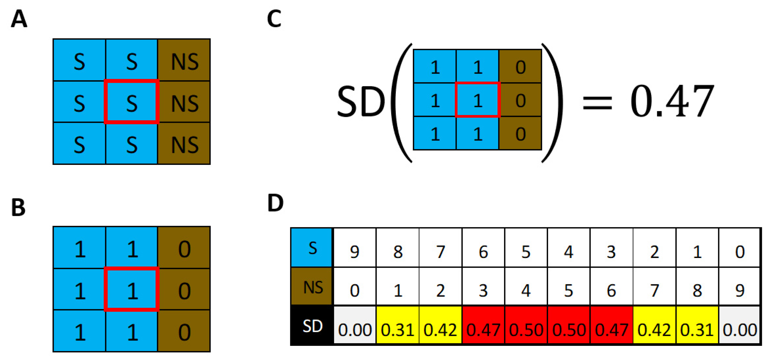
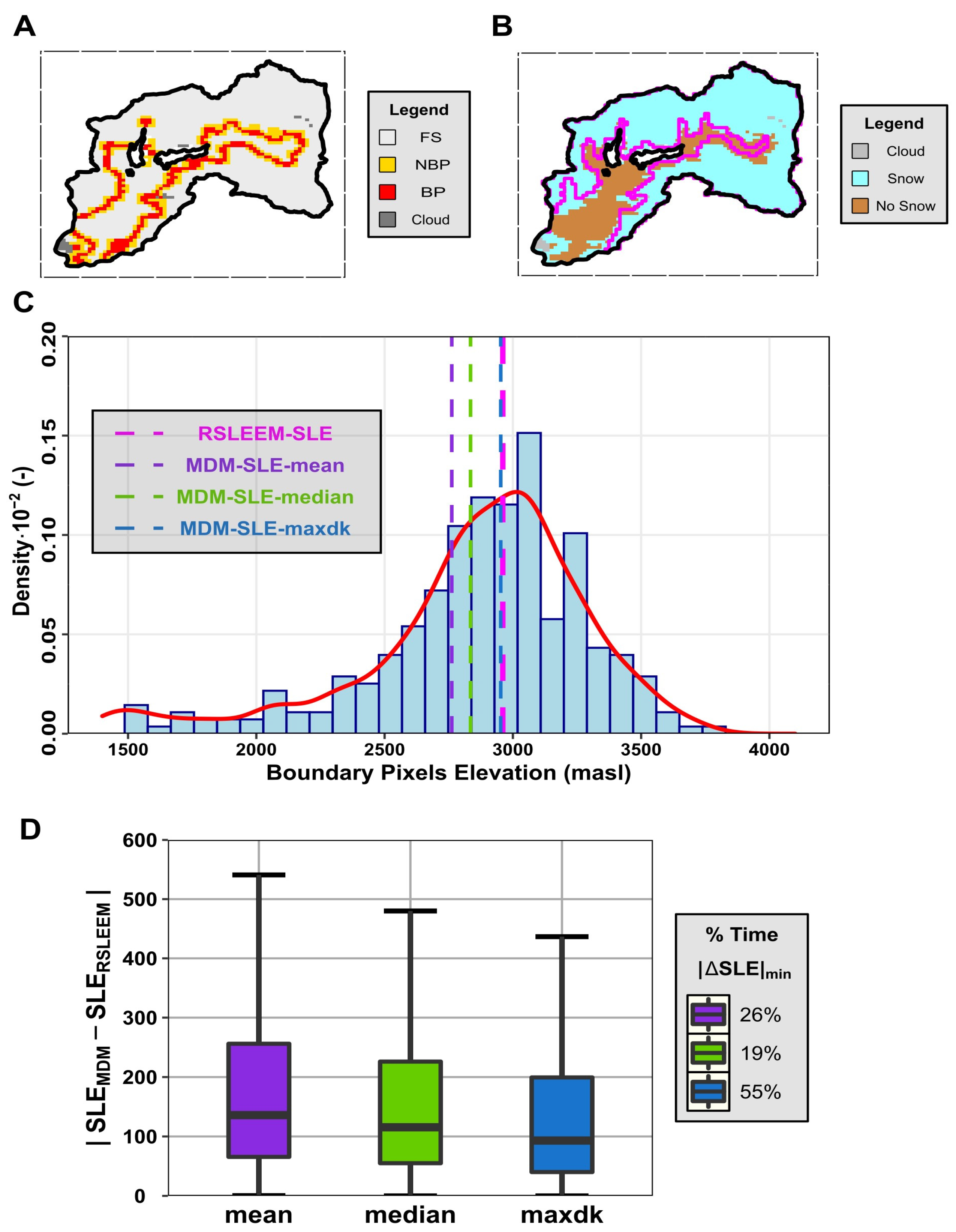
2.3.2. Snow Line Elevation
2.3.3. Snow Variables Trend and Their Correlations
3. Results and Discussion
3.1. Spatiotemporal Variation in the Snow Cover and Persistence
3.1.1. Elevation Bands Definition
3.1.2. Spatiotemporal Variation in Snow
3.2. Snow Persistence Trends
3.2.1. Temporal Variation in SP at Basin Scale
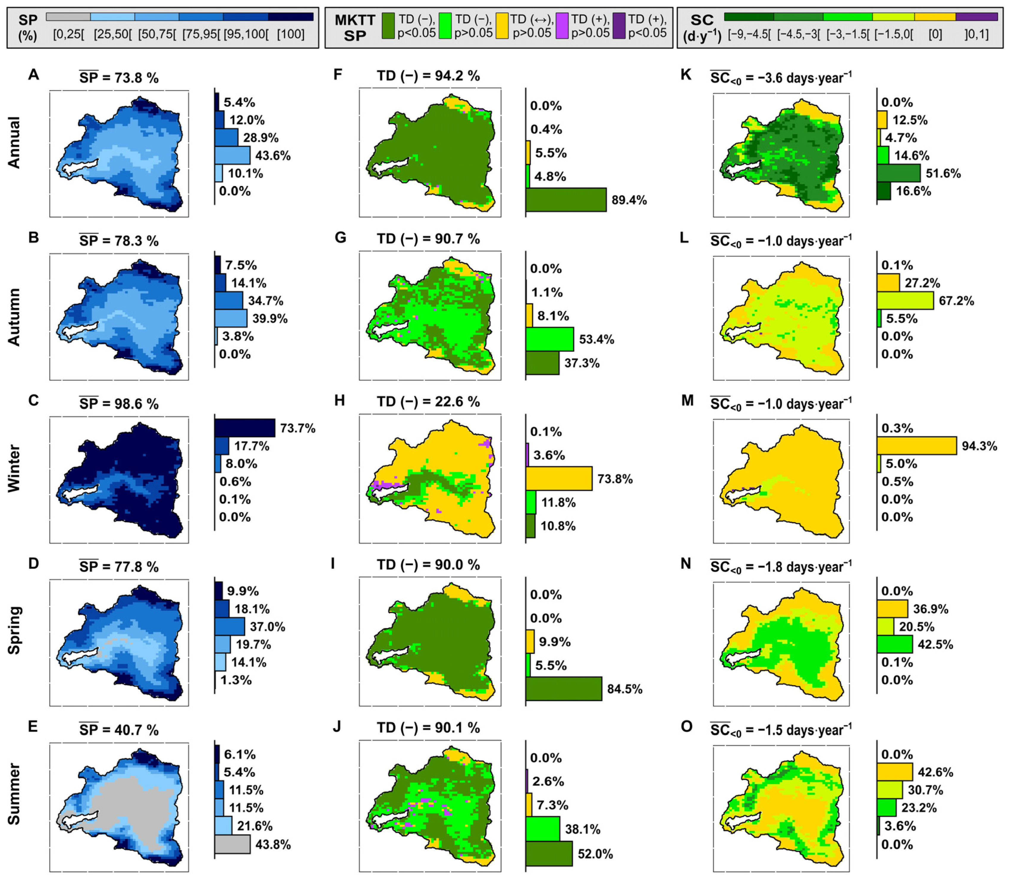
3.2.2. Spatial Distribution and Variation
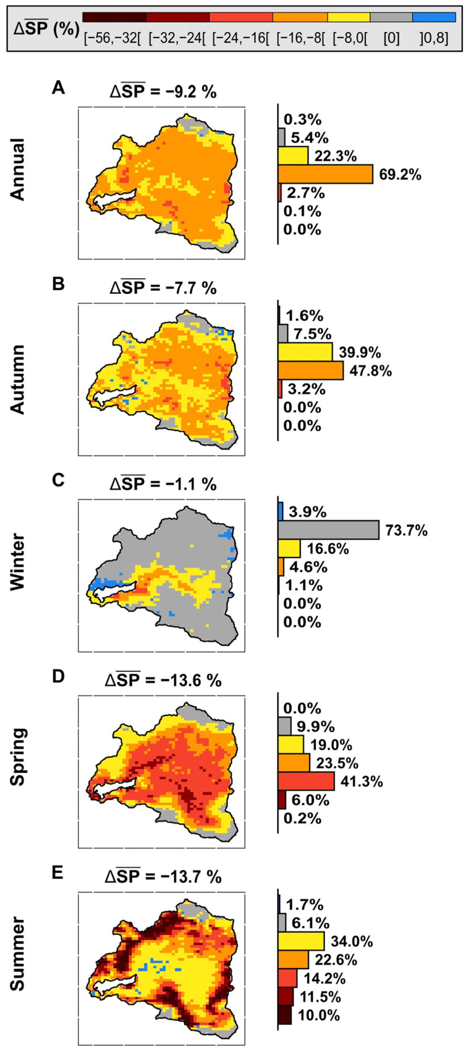
3.2.3. Change in SP between Pre and Megadrought Periods
3.3. Snow Line Elevation Trend
3.3.1. Temporal Variation in SLE
3.3.2. Interannual Variation in SLE
3.4. Correlation of Snow Variables with Hydrometeorological Variables and Large-Scale Climate Indices
3.4.1. Annual Correlation with SP
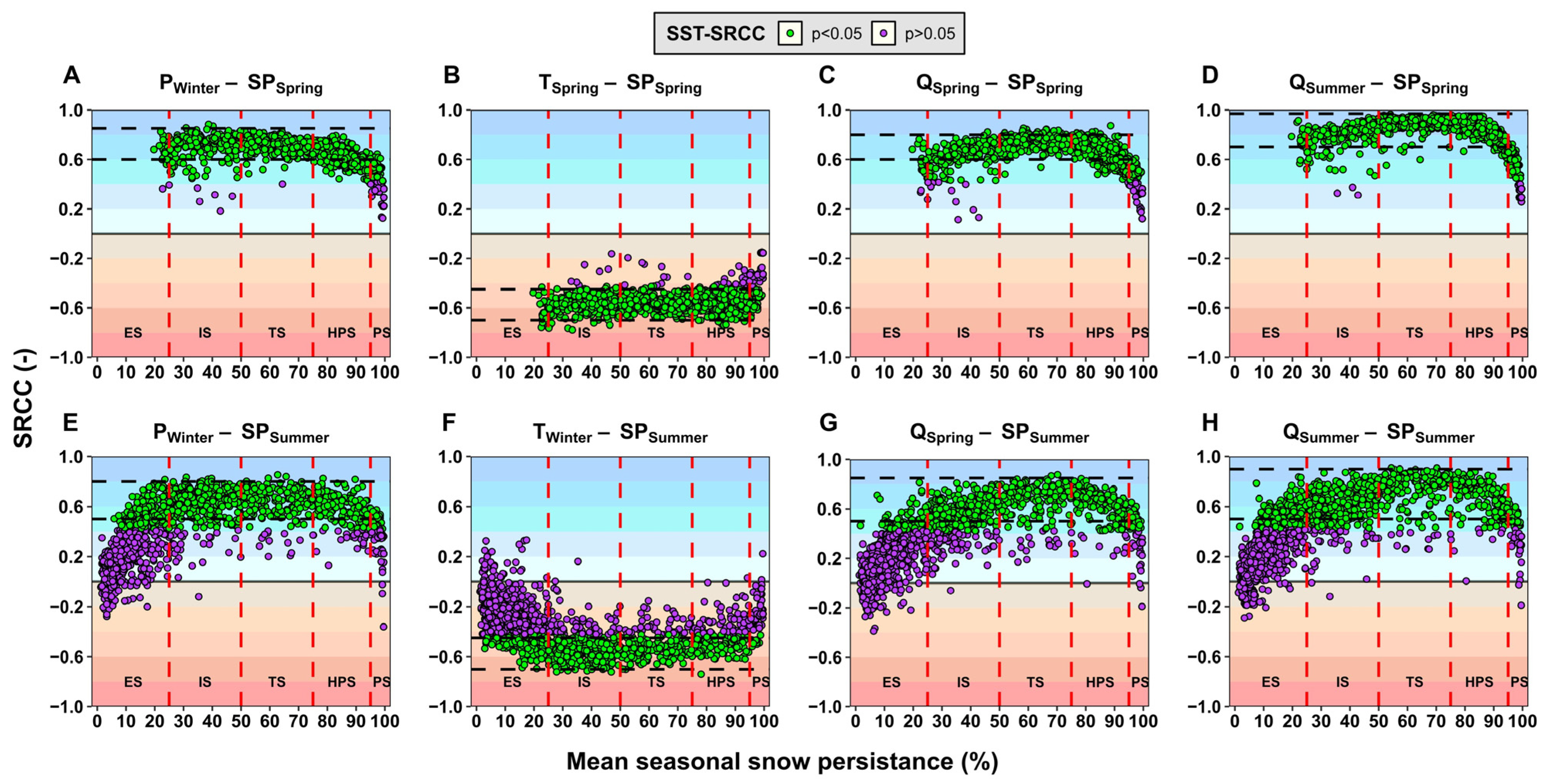
3.4.2. Seasonal Correlation with SP
3.4.3. Annual Correlation with Snow Variables at Basin Spatial Scale
4. Conclusions
Author Contributions
Funding
Data Availability Statement
Acknowledgments
Conflicts of Interest
Appendix A

| Period | Days of the Year | Season | Time Step | Initial Date | Final Date |
|---|---|---|---|---|---|
| 1 | 1–8 | Summer | 36 | 01-January | 08-January |
| 2 | 9–16 | 37 | 09-January | 16-January | |
| 3 | 17–24 | 38 | 17-January | 24-January | |
| 4 | 25–32 | 39 | 25-January | 01-February | |
| 5 | 33–40 | 40 | 02-February | 09-February | |
| 6 | 41–48 | 41 | 10-February | 17-February | |
| 7 | 49–56 | 42 | 18-February | 25-February | |
| 8 | 57–64 | 43 | 26-February | 05-March | |
| 9 | 65–72 | 44 | 06-March | 13-March | |
| 10 | 73–80 | 45 | 14-March | 21-March | |
| 11 | 81–88 | 46 | 22-March | 29-March | |
| 12 | 89–96 | Autumn | 1 | 30-March | 06-April |
| 13 | 97–104 | 2 | 07-April | 14-April | |
| 14 | 105–112 | 3 | 15-April | 22-April | |
| 15 | 113–120 | 4 | 23-April | 30-April | |
| 16 | 121–128 | 5 | 01-May | 08-May | |
| 17 | 129–136 | 6 | 09-May | 16-May | |
| 18 | 137–144 | 7 | 17-May | 24-May | |
| 19 | 145–152 | 8 | 25-May | 01-June | |
| 20 | 153–160 | 9 | 02-June | 09-June | |
| 21 | 161–168 | 10 | 10-June | 17-June | |
| 22 | 169–176 | 11 | 18-June | 25-June | |
| 23 | 177–184 | 12 | 26-June | 03-July | |
| 24 | 185–192 | Winter | 13 | 04-July | 11-July |
| 25 | 193–200 | 14 | 12-July | 19-July | |
| 26 | 201–208 | 15 | 20-July | 27-July | |
| 27 | 209–216 | 16 | 28-July | 04-August | |
| 28 | 217–224 | 17 | 05-August | 12-August | |
| 29 | 225–232 | 18 | 13-August | 20-August | |
| 30 | 233–240 | 19 | 21-August | 28-August | |
| 31 | 241–248 | 20 | 29-August | 05-September | |
| 32 | 249–256 | 21 | 06-September | 13-September | |
| 33 | 257–264 | 22 | 14-September | 21-September | |
| 34 | 265–272 | 23 | 22-September | 29-September | |
| 35 | 273–280 | Spring | 24 | 30-September | 07-October |
| 36 | 281–288 | 25 | 08-October | 15-October | |
| 37 | 289–296 | 26 | 16-October | 23-October | |
| 38 | 297–304 | 27 | 24-October | 31-October | |
| 39 | 305–312 | 28 | 01-November | 08-November | |
| 40 | 313–320 | 29 | 09-November | 16-November | |
| 41 | 321–328 | 30 | 17-November | 24-November | |
| 42 | 329–336 | 31 | 25-November | 02-December | |
| 43 | 337–344 | 32 | 03-December | 10-December | |
| 44 | 345–352 | 33 | 11-December | 18-December | |
| 45 | 353–360 | 34 | 19-December | 26-December | |
| 46 | 361–368 * | 35 | 27-December | 03-January |
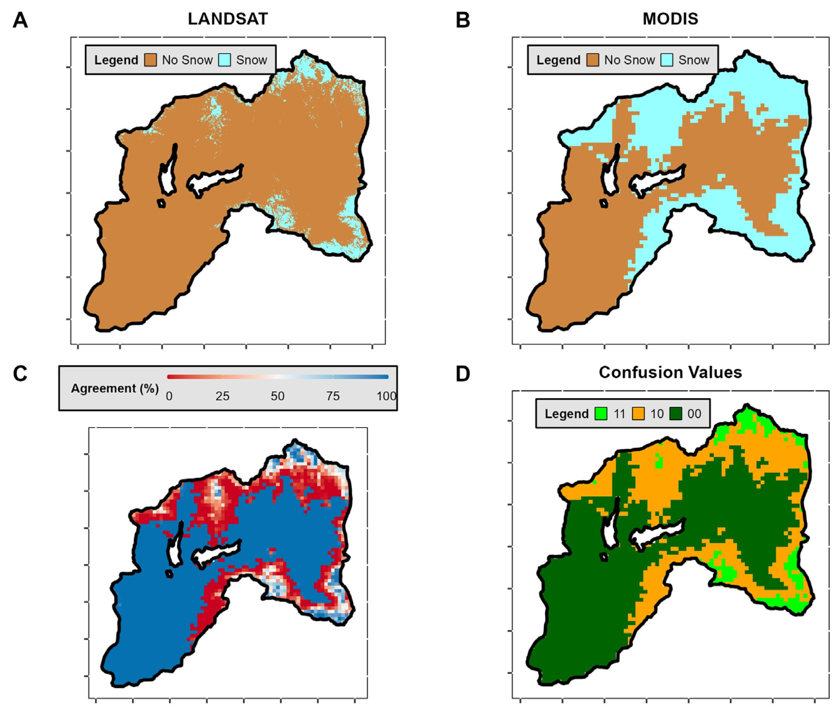
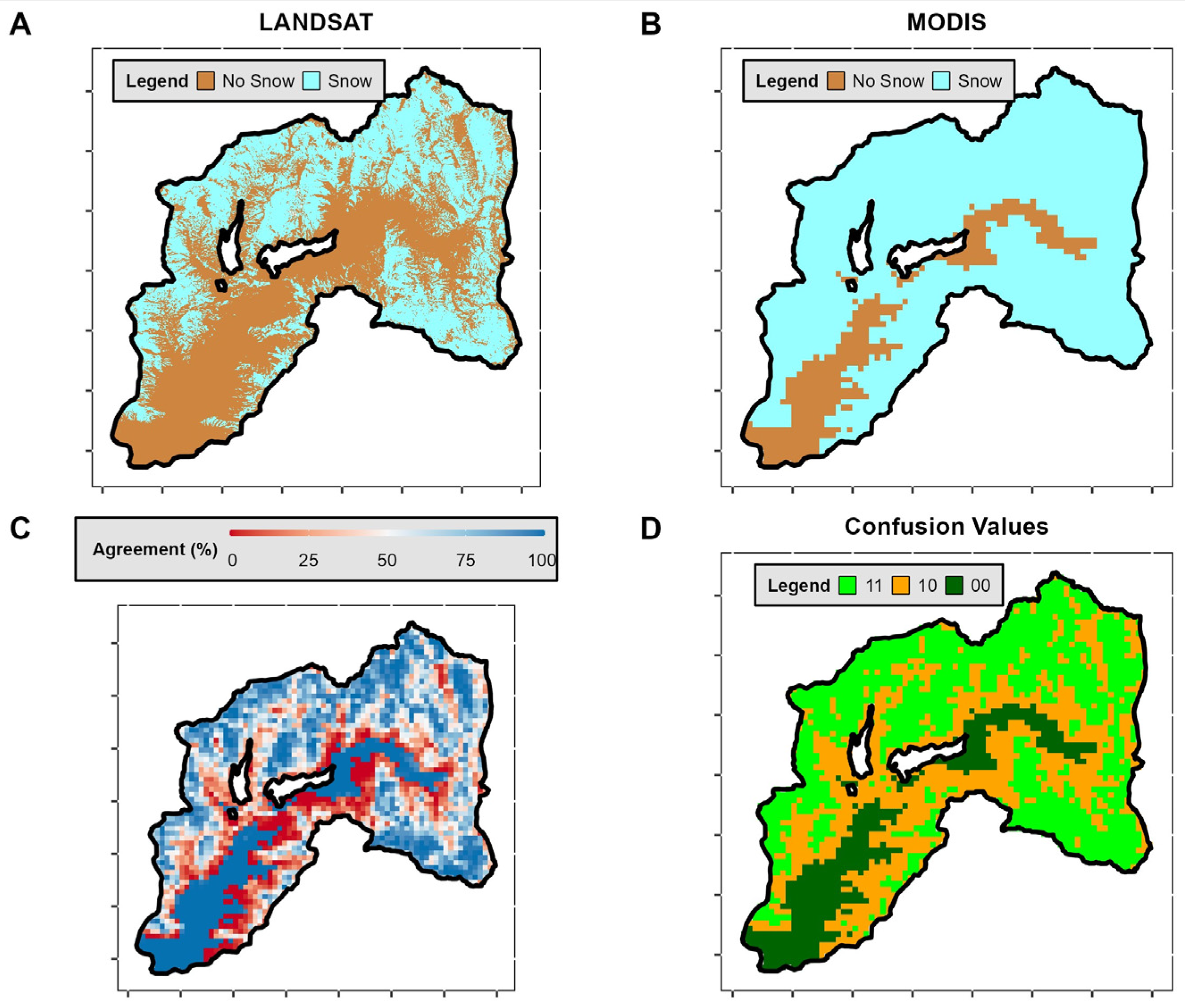
| Confusion Matrix | Landsat | ||
|---|---|---|---|
| Snow (1) | No Snow (0) | ||
| MODIS | Snow (1) | 11 | 10 |
| No Snow (0) | 01 | 00 | |
| CHY | Season | Figure | Date MODIS | Date Landsat-8 | Confusion Matrix Values | True +/− | False +/− | |||
|---|---|---|---|---|---|---|---|---|---|---|
| 11 | 10 | 01 | 00 | |||||||
| 2015 | Winter | Figure A1 | 23 July 2015 | 23 July 2015 | 2560 | 267 | 0 | 9 | 90.6% | 9.4% |
| Spring | Figure A2 | 12 December 2015 | 28 November 2015 | 1569 | 375 | 16 | 888 | 86.3% | 13.7% | |
| Summer | Figure A3 | 14 March 2016 | 19 March 2016 | 46 | 637 | 0 | 2168 | 77.7% | 22.3% | |
| 2020 | Winter | Figure A4 | 28 July 2020 | 29 July 2020 | 2596 | 243 | 0 | 9 | 91.5% | 8.5% |
| Spring | Figure A5 | 8 October 2020 | 8 October 2020 | 1336 | 1079 | 0 | 436 | 62.2% | 37.8% | |
| Summer | Figure A6 | 19 February 2021 | 22 February 2021 | 189 | 892 | 0 | 1769 | 68.7% | 31.3% | |
| Period | Elevation Band | Low (L): 2510–3410 masl | Low (L): 3410–4140 masl | Low (L): 4140–6000 masl | |||||||||
|---|---|---|---|---|---|---|---|---|---|---|---|---|---|
| SP (%) | 25–50 | 50–75 | 75–95 | >95 | 25–50 | 50–75 | 75–95 | >95 | 25–50 | 50–75 | 75–95 | >95 | |
| Range | IT | TS | HPS | PS | IT | TS | HPS | PS | IT | TS | HPS | PS | |
| Annual | 2000–2004 | 13.8 | 82.4 | 22.7 | 3.9 | 0.0 | 26.8 | 86.3 | 36.1 | 0.0 | 0.0 | 13.2 | 54.7 |
| 2005–2009 | 17.5 | 84.6 | 17.1 | 3.7 | 0.0 | 37.2 | 76.3 | 35.7 | 0.0 | 0.0 | 14.3 | 53.6 | |
| 2010–2015 | 49.5 | 64.9 | 7.1 | 1.3 | 0.6 | 89.3 | 47.1 | 12.1 | 0.0 | 3.9 | 20.5 | 43.5 | |
| 2016–2021 | 61.0 | 55.6 | 5.4 | 0.9 | 2.8 | 106.0 | 34.4 | 6.1 | 0.0 | 9.1 | 24.9 | 34.0 | |
| Autumn | 2000–2004 | 3.2 | 70.9 | 40.4 | 8.2 | 0.0 | 8.0 | 88.4 | 52.8 | 0.0 | 0.0 | 10.2 | 57.7 |
| 2005–2009 | 10.4 | 84.6 | 21.2 | 6.7 | 0.0 | 27.0 | 87.6 | 34.6 | 0.0 | 0.6 | 17.9 | 49.3 | |
| 2010–2015 | 26.2 | 78.1 | 14.5 | 4.1 | 0.0 | 72.0 | 59.0 | 18.2 | 0.0 | 4.1 | 18.8 | 45.0 | |
| 2016–2021 | 13.8 | 92.1 | 13.2 | 3.5 | 0.0 | 83.5 | 50.8 | 14.9 | 0.0 | 4.8 | 23.1 | 40.0 | |
| Winter | 2000–2004 | 0.2 | 0.6 | 11.0 | 110.9 | 0.0 | 0.0 | 0.0 | 149.2 | 0.0 | 0.0 | 0.0 | 67.9 |
| 2005–2009 | 0.2 | 0.9 | 6.7 | 115.0 | 0.0 | 0.0 | 0.2 | 149.0 | 0.0 | 0.0 | 0.0 | 67.9 | |
| 2010–2015 | 0.2 | 1.9 | 24.2 | 96.4 | 0.0 | 0.0 | 0.2 | 149.0 | 0.0 | 0.0 | 0.0 | 67.9 | |
| 2016–2021 | 0.9 | 9.1 | 31.4 | 81.5 | 0.0 | 0.2 | 3.7 | 145.3 | 0.0 | 0.0 | 0.0 | 67.9 | |
| Spring | 2000–2004 | 21.6 | 44.5 | 40.7 | 15.8 | 0.2 | 3.5 | 40.0 | 105.5 | 0.0 | 0.0 | 0.0 | 67.9 |
| 2005–2009 | 25.5 | 42.2 | 36.8 | 18.4 | 0.2 | 3.9 | 37.0 | 108.1 | 0.0 | 0.0 | 0.0 | 67.9 | |
| 2010–2015 | 49.5 | 38.7 | 17.3 | 3.7 | 3.7 | 32.7 | 70.5 | 42.4 | 0.0 | 0.2 | 11.0 | 56.7 | |
| 2016–2021 | 49.7 | 29.4 | 8.7 | 1.1 | 13.8 | 70.5 | 54.5 | 10.2 | 0.0 | 5.8 | 22.3 | 39.8 | |
| Summer | 2000–2004 | 17.3 | 9.5 | 3.7 | 2.2 | 48.9 | 32.2 | 21.6 | 21.0 | 2.4 | 8.0 | 10.4 | 47.1 |
| 2005–2009 | 13.0 | 8.2 | 3.2 | 2.2 | 45.2 | 26.4 | 21.6 | 24.0 | 2.8 | 6.7 | 8.0 | 50.4 | |
| 2010–2015 | 7.1 | 2.2 | 2.2 | 0.6 | 42.8 | 17.7 | 10.4 | 5.8 | 9.7 | 9.3 | 14.1 | 34.6 | |
| 2016–2021 | 8.9 | 1.7 | 2.4 | 0.2 | 34.4 | 14.7 | 7.6 | 2.4 | 10.2 | 15.1 | 12.1 | 28.1 | |
| SP Time Scale | Variable Time Scale | SP (%) | 0–25% | 25–50% | 50–75% | 75–95% | >95% | 100% | |||||
|---|---|---|---|---|---|---|---|---|---|---|---|---|---|
| SPZ | ES | IT | TS | HPS | PS | - | |||||||
| Variable | p > 0.05 | p < 0.05 | p > 0.05 | p < 0.05 | p > 0.05 | p < 0.05 | p > 0.05 | p < 0.05 | p > 0.05 | p < 0.05 | - | ||
| Annual | Annual | P | 0.0% | 0.0% | 0.1% | 9.9% | 0.0% | 43.8% | 0.0% | 28.8% | 3.4% | 8.7% | 5.4% |
| Annual | T | 0.0% | 0.0% | 0.2% | 9.8% | 0.0% | 43.8% | 0.6% | 28.1% | 3.7% | 8.3% | 5.4% | |
| Annual | Q | 0.0% | 0.0% | 3.4% | 6.6% | 3.8% | 40.1% | 3.8% | 25.0% | 8.7% | 3.3% | 5.4% | |
| MJM | MEI | 0.0% | 0.0% | 9.7% | 0.4% | 37.8% | 5.7% | 24.5% | 4.4% | 11.6% | 0.4% | 5.4% | |
| MJM | SOI | 0.0% | 0.0% | 9.9% | 0.2% | 43.6% | 0.0% | 28.9% | 0.0% | 12.0% | 0.0% | 5.4% | |
| MAM | AAO | 0.0% | 0.0% | 10.1% | 0.0% | 42.9% | 0.6% | 27.7% | 1.2% | 10.2% | 1.8% | 5.4% | |
| Total | 0.0% | 10.1% | 43.6% | 28.9% | 12.0% | 5.4% | |||||||
| Spring | Winter | P | 0.1% | 1.2% | 0.4% | 13.7% | 0.1% | 19.6% | 0.1% | 36.9% | 6.3% | 11.8% | 9.9% |
| Spring | T | 0.0% | 1.3% | 0.4% | 13.6% | 0.6% | 19.0% | 1.6% | 35.4% | 11.0% | 7.1% | 9.9% | |
| Spring | Q | 0.1% | 1.1% | 0.8% | 13.3% | 0.0% | 19.7% | 0.1% | 36.9% | 5.9% | 12.2% | 9.9% | |
| Summer | Q | 0.0% | 1.3% | 0.2% | 13.9% | 0.0% | 19.7% | 0.0% | 37.0% | 3.2% | 14.9% | 9.9% | |
| Total | 1.3% | 14.1% | 19.7% | 37.0% | 18.1% | 9.9% | |||||||
| Summer | Winter | P | 33.0% | 11.1% | 1.9% | 19.5% | 0.8% | 10.7% | 1.7% | 9.8% | 4.0% | 1.4% | 6.1% |
| Winter | T | 35.7% | 8.3% | 4.1% | 17.3% | 2.6% | 8.9% | 4.8% | 6.7% | 4.7% | 0.7% | 6.1% | |
| Spring | Q | 37.7% | 6.4% | 5.0% | 16.5% | 1.0% | 10.5% | 0.8% | 10.7% | 2.8% | 2.6% | 6.1% | |
| Summer | Q | 32.7% | 11.3% | 2.4% | 19.1% | 0.7% | 10.8% | 0.6% | 10.9% | 2.7% | 2.7% | 6.1% | |
| Total | 44.0% | 21.4% | 11.5% | 11.5% | 5.4% | 6.1% | |||||||


References
- Beniston, M. Impacts of climatic change on water and associated economic activities in the Swiss Alps. J. Hydrol. 2012, 412–413, 291–296. [Google Scholar] [CrossRef]
- Meza, F.J.; Wilks, D.S.; Gurovich, L.; Bambach, N. Impacts of Climate Change on Irrigated Agriculture in the Maipo Basin, Chile: Reliability of Water Rights and Changes in the Demand for Irrigation. J. Water Resour. Plan. Manag. 2012, 138, 421–430. [Google Scholar] [CrossRef]
- Su, B.; Xiao, C.; Chen, D.; Qin, D.; Ding, Y. Cryosphere services and human well-being. Sustainability 2019, 11, 4365. [Google Scholar] [CrossRef]
- Masiokas, M.; Villalba, R.; Luckman, B.H.; Le Quesne, C.; Aravena, J.C. Snowpack variations in the central Andes of Argentina and Chile, 1951–2005: Large-scale atmospheric influences and implications for water resources in the region. J. Clim. 2006, 19, 6334–6352. [Google Scholar] [CrossRef]
- Meza, F.J.; Vicuña, S.; Jelinek, M.; Bustos, E.; Bonelli, S. Assessing water demands and coverage sensitivity to climate change in the urban and rural sectors in central Chile. J. Water Clim. Chang. 2014, 5, 192–203. [Google Scholar] [CrossRef]
- Deser, C.; Phillips, A.; Bourdette, V.; Teng, H. Uncertainty in climate change projections: The role of internal variability. Clim. Dyn. 2012, 38, 527–546. [Google Scholar] [CrossRef]
- Barrett, B.S.; Garreaud, R.D.; Falvey, M. Effect of the Andes Cordillera on precipitation from a midlatitude cold front. Mon. Weather Rev. 2009, 137, 3092–3109. [Google Scholar] [CrossRef]
- Klos, P.Z.; Link, T.E.; Abatzoglou, J.T. Extent of the rain-snow transition zone in the western U.S. under historic and projected climate. Geophys. Res. Lett. 2014, 41, 4560–4568. [Google Scholar] [CrossRef]
- Mardones, P.; Garreaud, R.D. Future changes in the free tropospheric freezing level and rain–snow limit: The case of central Chile. Atmosphere 2020, 11, 1259. [Google Scholar] [CrossRef]
- Masson-Delmotte, V.; Zhai, P.; Pirani, A.; Connors, S.L.; Péan, C.; Berger, S.; Caud, N.; Chen, Y.; Goldfarb, L.; Gomis, M.I.; et al. IPCC: Climate Change 2021: The Physical Science Basis; Cambridge University Press: Cambridge, UK, 2021. [Google Scholar]
- Burger, F.; Brock, B.; Montecinos, A. Seasonal and elevational contrasts in temperature trends in Central Chile between 1979 and 2015. Glob. Planet. Chang. 2018, 162, 136–147. [Google Scholar] [CrossRef]
- Saavedra, F.A.; Kampf, S.K.; Fassnacht, S.R.; Sibold, J.S. Changes in Andes snow cover from MODIS data, 2000–2016. Cryosphere 2018, 12, 1027–1046. [Google Scholar] [CrossRef]
- Barnett, T.P.; Adam, J.C.; Lettenmaier, D.P. Potential impacts of a warming climate on water availability in snow-dominated regions. Nature 2005, 438, 303–309. [Google Scholar] [CrossRef] [PubMed]
- Huss, M.; Bookhagen, B.; Huggel, C.; Jacobsen, D.; Bradley, R.; Clague, J.; Vuille, M.; Buytaert, W.; Cayan, D.; Greenwood, G.; et al. Towards mountains without permanent snow and ice: Mountains without permanent snow and ice. Earth’s Future 2017, 5, 418–435. [Google Scholar] [CrossRef]
- Masiokas, M.; Rabatel, A.; Rivera, A.; Ruiz, L.; Pitte, P.; Ceballos, J.L.; Barcaza, G.; Soruco, A.; Bown, F.; Berthier, E.; et al. A Review of the Current State and Recent Changes of the Andean Cryosphere. Front. Earth Sci. 2020, 8, 99. [Google Scholar] [CrossRef]
- Demaria, E.M.C.; Maurer, E.P.; Thrasher, B.; Vicuña, S.; Meza, F.J. Climate change impacts on an alpine watershed in Chile: Do new model projections change the story? J. Hydrol. 2013, 502, 128–138. [Google Scholar] [CrossRef]
- Migliavacca, F.; Confortola, G.; Soncini, A.; Senese, A.; Diolaiuti, G.A.; Smiraglia, C.; Barcaza, G.; Bocchiola, D. Hydrology and potential climate changes in the Rio Maipo (Chile). Geogr. Fis. E Din. Quat. 2015, 38, 155–168. [Google Scholar] [CrossRef]
- Richer, E.E.; Kampf, S.K.; Fassnacht, S.R.; Moore, C.C. Spatiotemporal index for analyzing controls on snow climatology: Application in the Colorado Front Range. Phys. Geogr. 2013, 34, 85–107. [Google Scholar] [CrossRef]
- Tang, Z.; Wang, X.; Wang, J.; Wang, X.; Li, H.; Jiang, Z. Spatiotemporal variation of snow cover in Tianshan Mountains, Central Asia, based on cloud-free MODIS fractional snow cover product, 2001–2015. Remote Sens. 2017, 9, 1045. [Google Scholar] [CrossRef]
- Dozier, J. Spectral signature of alpine snow cover from the landsat thematic mapper. Remote Sens. Environ. 1989, 28, 9–22. [Google Scholar] [CrossRef]
- Dietz, A.J.; Kuenzer, C.; Gessner, U.; Dech, S. Remote sensing of snow—A review of available methods. Int. J. Remote Sens. 2012, 33, 4094–4134. [Google Scholar] [CrossRef]
- Notarnicola, C. Overall negative trends for snow cover extent and duration in global mountain regions over 1982–2020. Sci. Rep. 2022, 12, 13731. [Google Scholar] [CrossRef] [PubMed]
- Hammond, J.C.; Saavedra, F.A.; Kampf, S.K. Global snow zone maps and trends in snow persistence 2001–2016. Int. J. Climatol. 2018, 38, 4369–4383. [Google Scholar] [CrossRef]
- O’Leary, D.S.; Hall, D.K.; DiGirolamo, N.E.; Riggs, G.A. Regional trends in snowmelt timing for the western United States throughout the MODIS era. Phys. Geogr. 2022, 43, 285–307. [Google Scholar] [CrossRef]
- Tang, Z.; Wang, J.; Li, H.; Liang, J.; Li, C.; Wang, X. Extraction and assessment of snowline altitude over the Tibetan plateau using MODIS fractional snow cover data (2001 to 2013). J. Appl. Remote Sens. 2014, 8, 084689. [Google Scholar] [CrossRef]
- Racoviteanu, A.E.; Rittger, K.; Armstrong, R. An Automated Approach for Estimating Snowline Altitudes in the Karakoram and Eastern Himalaya From Remote Sensing. Front. Earth Sci. 2019, 7, 220. [Google Scholar] [CrossRef]
- Krajčí, P.; Holko, L.; Perdigão, R.A.P.; Parajka, J. Estimation of regional snowline elevation (RSLE) from MODIS images for seasonally snow covered mountain basins. J. Hydrol. 2014, 519, 1769–1778. [Google Scholar] [CrossRef]
- Khadka, N.; Khadka, N.; Ghimire, S.K.; Chen, X.; Thakuri, S.; Hamal, K.; Shrestha, D.; Sharma, S. Dynamics of Maximum Snow Cover Area and Snow Line Altitude Across Nepal (2003–2018) Using Improved MODIS Data. J. Inst. Sci. Technol. 2020, 25, 17–24. [Google Scholar] [CrossRef]
- Thapa, A.; Muhammad, S. Contemporary snow changes in the karakoram region attributed to improved modis data between 2003 and 2018. Water 2020, 12, 2681. [Google Scholar] [CrossRef]
- Chávez, R.O.; Briceño, V.F.; Lastra, J.A.; Harris-Pascal, D.; Estay, S.A. Snow Cover and Snow Persistence Changes in the Mocho-Choshuenco Volcano (Southern Chile) Derived From 35 Years of Landsat Satellite Images. Front. Ecol. Evol. 2021, 9, 643850. [Google Scholar] [CrossRef]
- Pérez, T.; Mattar, C.; Fuster, R. Decrease in snow cover over the Aysén river catchment in Patagonia, Chile. Water 2018, 10, 619. [Google Scholar] [CrossRef]
- Bevington, A.R.; Gleason, H.E.; Foord, V.N.; Floyd, W.C.; Griesbauer, H.P. Regional influence of ocean-atmosphere teleconnections on the timing and duration of MODIS-derived snow cover in British Columbia, Canada. Cryosphere 2019, 13, 2693–2712. [Google Scholar] [CrossRef]
- Zalazar, L.; Ferri, L.; Castro, M.; Gargantini, H.; Gimenez, M.; Pitte, P.; Ruiz, L.; Masiokas, M.; Costa, G.; Villalba, R. Spatial distribution and characteristics of Andean ice masses in Argentina: Results from the first National Glacier Inventory. J. Glaciol. 2020, 66, 938–949. [Google Scholar] [CrossRef]
- Kunkel, K.E.; Angel, J.R. Relationship of ENSO to snowfall and related cyclone activity in the contiguous United States. J. Geophys. Res. Atmos. 1999, 104, 19425–19434. [Google Scholar] [CrossRef]
- Escobar, F.; Aceituno, P. Influencia del fenómeno ENSO sobre la precipitación nival en el sector andino de Chile Central durante el invierno. Bull. L’inst. Fr. D’études Andin. 1998, 27, 753–759. [Google Scholar] [CrossRef]
- Wang, Z.; Wu, R.; Yang, S.; Lu, M. An Interdecadal Change in the Influence of ENSO on the Spring Tibetan Plateau Snow-Cover Variability in the Early 2000s. J. Clim. 2022, 35, 725–743. [Google Scholar] [CrossRef]
- Shaman, J.; Tziperman, E. The effect of ENSO on Tibetan Plateau snow depth: A stationary wave teleconnection mechanism and implications for the south Asian monsoons. J. Clim. 2005, 18, 2067–2079. [Google Scholar] [CrossRef]
- Marshall, G.J. Trends in the Southern Annular Mode from observations and reanalyses. J. Clim. 2003, 16, 4134–4143. [Google Scholar] [CrossRef]
- Montecinos, A.; Aceituno, P. Seasonality of the ENSO-related rainfall variability in central Chile and associated circulation anomalies. J. Clim. 2003, 16, 281–296. [Google Scholar] [CrossRef]
- Masiokas, M.; Christie, D.A.; Le Quesne, C.; Pitte, P.; Ruiz, L.; Villalba, R.; Luckman, B.H.; Berthier, E.; Nussbaumer, S.U.; González-Reyes, Á.; et al. Reconstructing the annual mass balance of the Echaurren Norte glacier (Central Andes, 33.5°S) using local and regional hydroclimatic data. Cryosphere 2016, 10, 927–940. [Google Scholar] [CrossRef]
- Boisier, J.P.; Alvarez-Garreton, C.; Cordero, R.R.; Damiani, A.; Gallardo, L.; Garreaud, R.D.; Lambert, F.; Ramallo, C.; Rojas, M.; Rondanelli, R. Anthropogenic drying in central-southern Chile evidenced by long-term observations and climate model simulations. Elementa 2018, 6, 74. [Google Scholar] [CrossRef]
- Xu, K.; Brown, C.; Kwon, H.H.; Lall, U.; Zhang, J.; Hayashi, S.; Chen, Z. Climate teleconnections to Yangtze river seasonal streamflow at the Three Gorges Dam, China. Int. J. Climatol. 2007, 27, 771–780. [Google Scholar] [CrossRef]
- Ossandón, Á.; Brunner, M.I.; Rajagopalan, B.; Kleiber, W. A space-time Bayesian hierarchical modeling framework for projection of seasonal maximum streamflow. Hydrol. Earth Syst. Sci. 2022, 26, 149–166. [Google Scholar] [CrossRef]
- Maurer, E.P.; Lettenmaier, D.P.; Mantua, N.J. Variability and potential sources of predictability of North American runoff. Water Resour. Res. 2004, 40, W09306. [Google Scholar] [CrossRef]
- Le, E.; Ameli, A.A.; Janssen, J.; Hammond, J. Snow Persistence Explains Stream High Flow and Low Flow Signatures with Differing Relationships by Aridity and Climatic Seasonality. Hydrol. Earth Syst. Sci. 2022, 1–22. [Google Scholar]
- Stehr, A.; Aguayo, M. Snow cover dynamics in Andean watersheds of Chile (32.0–39.5°S) during the years 2000–2016. Hydrol. Earth Syst. Sci. 2017, 21, 5111–5126. [Google Scholar] [CrossRef]
- Alvarez-Garreton, C.; Pablo Boisier, J.; Garreaud, R.; Seibert, J.; Vis, M. Progressive water deficits during multiyear droughts in basins with long hydrological memory in Chile. Hydrol. Earth Syst. Sci. 2021, 25, 429–446. [Google Scholar] [CrossRef]
- Montaner-Fernández, D.; Morales-Salinas, L.; Rodriguez, J.S.; Cárdenas-Jirón, L.; Huete, A.; Fuentes-Jaque, G.; Pérez-Martínez, W.; Cabezas, J. Spatio-temporal variation of the urban heat island in Santiago, Chile during summers 2005–2017. Remote Sens. 2020, 12, 3345. [Google Scholar] [CrossRef]
- Uribe, F. Comparación De La Cobertura Nival E Hidrogramas Simulados a Distintas Escalas Temporales En La Cuenca Alta Del Río Maipo, Por Distintas Conceptualizaciones Del Proceso Nival; Universidad de Chile: Santiago, Chile, 2015; p. 78. [Google Scholar]
- Falvey, M.; Garreaud, R. Wintertime precipitation episodes in Central Chile: Associated meteorological conditions and orographic influences. J. Hydrometeorol. 2007, 8, 171–193. [Google Scholar] [CrossRef]
- Falvey, M.; Garreaud, R. Regional cooling in a warming world: Recent temperature trends in the southeast Pacific and along the west coast of subtropical South America (1979–2006). J. Geophys. Res. Atmos. 2009, 114, 1–16. [Google Scholar] [CrossRef]
- Garreaud, R.D.; Boisier, J.P.; Rondanelli, R.; Montecinos, A.; Sepúlveda, H.H.; Veloso-Aguila, D. The Central Chile Mega Drought (2010–2018): A climate dynamics perspective. Int. J. Climatol. 2020, 40, 421–439. [Google Scholar] [CrossRef]
- Boisier, J.P.; Rondanelli, R.; Garreaud, R.D.; Muñoz, F. Anthropogenic and natural contributions to the Southeast Pacific precipitation decline and recent megadrought in central Chile. Geophys. Res. Lett. 2016, 43, 413–421. [Google Scholar] [CrossRef]
- Hall, D.K.; Riggs, G.A. MODIS/Terra Snow Cover 8-Day L3 Global 500m Grid, Version 61 (MOD10A2); NASA National Snow and Ice Data Center: Boulder, CO, USA, 2021. [CrossRef]
- Dadashi, S.; Matkan, A.; Ziaiian, P.; Ashorlo, D. Evaluation of Pixelbase and Subpixel Methods for Snow Cover Studying in Regional Scale. In Proceedings of the 65th Eastern Snow Conference, Fairlee, VT, USA, 28–30 May 2008. [Google Scholar]
- Farr, T.G.; Rosen, P.A.; Caro, E.; Crippen, R.; Duren, R.; Hensley, S.; Kobrick, M.; Paller, M.; Rodriguez, E.; Roth, L.; et al. The shuttle radar topography mission. Rev. Geophys. 2007, 45, RG2004. [Google Scholar] [CrossRef]
- Aceituno, P. El Niño, the Southern Oscillation, and ENSO: Confusing Names for a Complex Ocean–Atmosphere Interaction. Bull. Am. Meteorol. Soc. 1992, 73, 483–485. [Google Scholar] [CrossRef][Green Version]
- Moore, C.; Kampf, S.; Stone, B.; Richer, E. A GIS-based method for defining snow zones: Application to the western United States. Geocarto Int. 2015, 30, 62–81. [Google Scholar] [CrossRef]
- Saavedra, F.A.; Kampf, S.K.; Fassnacht, S.R.; Sibold, J.S. A snow climatology of the Andes Mountains from MODIS snow cover data. Int. J. Climatol. 2017, 37, 1526–1539. [Google Scholar] [CrossRef]
- Lei, L.; Zeng, Z.; Zhang, B. Method for detecting snow lines from MODIS data and assessment of changes in the nianqingtanglha mountains of the Tibet Plateau. IEEE J. Sel. Top. Appl. Earth Obs. Remote Sens. 2012, 5, 769–776. [Google Scholar] [CrossRef]
- Kendall, M. Charles Griffin; Holden Day: San Francisco, CA, USA, 1975. [Google Scholar]
- Mann, H.B. Nonparametric tests against trend. Econom. J. Econom. Soc. 1945, 13, 245–259. [Google Scholar] [CrossRef]
- Atta-ur-Rahman; Dawood, M. Spatio-statistical analysis of temperature fluctuation using Mann–Kendall and Sen’s slope approach. Clim. Dyn. 2017, 48, 783–797. [Google Scholar] [CrossRef]
- Ke, C.Q.; Yu, T.; Yu, K.; Tang, G.D.; King, L. Snowfall trends and variability in Qinghai, China. Theor. Appl. Climatol. 2009, 98, 251–258. [Google Scholar] [CrossRef]
- Ali, R.O.; Abubaker, S.R. Trend analysis using mann-kendall, sen’s slope estimator test and innovative trend analysis method in Yangtze river basin, China: Review. Int. J. Eng. Technol. 2019, 8, 110–119. [Google Scholar]
- Sen, P.K. Estimates of the Regression Coefficient Based on Kendall’s Tau. J. Am. Stat. Assoc. 1968, 63, 1379–1389. [Google Scholar] [CrossRef]
- Glasser, G.J.; Winter, R.F. Critical Values of the Coefficient of Rank Correlation for Testing the Hypothesis of Independence. Biometrika 1961, 48, 444. [Google Scholar] [CrossRef]
- Saydi, M.; Ding, J. li Impacts of topographic factors on regional snow cover characteristics. Water Sci. Eng. 2020, 13, 171–180. [Google Scholar] [CrossRef]
- Garreaud, R.; Alvarez-Garreton, C.; Barichivich, J.; Pablo Boisier, J.; Christie, D.; Galleguillos, M.; LeQuesne, C.; McPhee, J.; Zambrano-Bigiarini, M. The 2010–2015 megadrought in central Chile: Impacts on regional hydroclimate and vegetation. Hydrol. Earth Syst. Sci. 2017, 21, 6307–6327. [Google Scholar] [CrossRef]
- DGA. Estrategia Nacional de Glaciares Fundamentos; Ministerio de Obras Públicas, Dirección General de Aguas: Santiago, Chile, 2009.
- Malmros, J.K.; Mernild, S.H.; Wilson, R.; Tagesson, T.; Fensholt, R. Snow cover and snow albedo changes in the central Andes of Chile and Argentina from daily MODIS observations (2000–2016). Remote Sens. Environ. 2018, 209, 240–252. [Google Scholar] [CrossRef]
- Notarnicola, C. Hotspots of snow cover changes in global mountain regions over 2000–2018. Remote Sens. Environ. 2020, 243, 111781. [Google Scholar] [CrossRef]
- Saavedra, F.; Cortés, G.; Viale, M.; Margulis, S.; McPhee, J. Atmospheric Rivers Contribution to the Snow Accumulation Over the Southern Andes (26.5–37.5°S). Front. Earth Sci. 2020, 8, 261. [Google Scholar] [CrossRef]
- Garreaud, R. Tres niños sorprendentes. Bol. Téc. Inst. Geofís. del Perú 2018, 5. [Google Scholar]
- Hrudya, P.H.; Varikoden, H.; Vishnu, R. A review on the Indian summer monsoon rainfall, variability and its association with ENSO and IOD. Meteorol. Atmos. Phys. 2021, 133, 1–14. [Google Scholar] [CrossRef]
- Kumar, K.K.; Rajagopalan, B.; Cane, M.A. On the weakening relationship between the indian monsoon and ENSO. Science 1999, 284, 2156–2159. [Google Scholar] [CrossRef]
- Yeh, S.W.; Cai, W.; Min, S.K.; McPhaden, M.J.; Dommenget, D.; Dewitte, B.; Collins, M.; Ashok, K.; An, S., II; Yim, B.Y.; et al. ENSO Atmospheric Teleconnections and Their Response to Greenhouse Gas Forcing. Rev. Geophys. 2018, 56, 185–206. [Google Scholar] [CrossRef]
- Reboita, M.S.; Ambrizzi, T.; Crespo, N.M.; Dutra, L.M.M.; Ferreira, G.W.d.S.; Rehbein, A.; Drumond, A.; da Rocha, R.P.; de Souza, C.A. Impacts of teleconnection patterns on South America climate. Ann. N. Y. Acad. Sci. 2021, 1504, 116–153. [Google Scholar] [CrossRef] [PubMed]


| Variable Name | Variable Abbreviation | Units | Institution | Temporal Resolution * | Available Data * |
|---|---|---|---|---|---|
| Precipitation | P | mm | DGA | Daily | 1962–2022 |
| Temperature | T | °C | DGA | Daily | 1962–2022 |
| Streamflow | Q | m3 s−1 | AA | Daily | 1996–2022 |
| Multivariate ENSO Index | MEI | - | NOAA | Monthly | 1979–2022 |
| Southern Oscillation Index | SOI | - | NOAA | Monthly | 1951–2022 |
| Annular Antarctic Oscillation | AAO | - | BAS | Monthly | 1957–2022 |
| Temporal Scale | Snow Variable | Temporal Scale | Hydrometeorological Variable | SRCC |
|---|---|---|---|---|
| Annual | SP | Annual | P | 0.88 * |
| Annual | SP | Annual | T | 0.55 * |
| Annual | SP | Annual | Q | 0.74 * |
| Annual | SLE | Annual | P | −0.35 |
| Annual | SLE | Annual | T | −0.20 |
| Annual | SLE | Annual | Q | −0.36 |
| Spring | SP | Winter | P | 0.72 * |
| Spring | SP | Spring | T | 0.61 * |
| Spring | SP | Spring | Q | 0.75 * |
| Spring | SP | Summer | Q | 0.93 * |
| Spring | SLE | Winter | P | −0.58 * |
| Spring | SLE | Winter | T | −0.39 |
| Spring | SLE | Spring | Q | −0.59 * |
| Spring | SLE | Summer | Q | −0.66 * |
| Summer | SP | Winter | P | 0.63 * |
| Summer | SP | Winter | T | 0.43 * |
| Summer | SP | Spring | Q | 0.62 * |
| Summer | SP | Summer | Q | 0.71 * |
| Summer | SLE | Winter | P | −0.63 * |
| Summer | SLE | Winter | T | −0.30 |
| Summer | SLE | Spring | Q | −0.83 * |
| Summer | SLE | Summer | Q | −0.84 * |
Disclaimer/Publisher’s Note: The statements, opinions and data contained in all publications are solely those of the individual author(s) and contributor(s) and not of MDPI and/or the editor(s). MDPI and/or the editor(s) disclaim responsibility for any injury to people or property resulting from any ideas, methods, instructions or products referred to in the content. |
© 2023 by the authors. Licensee MDPI, Basel, Switzerland. This article is an open access article distributed under the terms and conditions of the Creative Commons Attribution (CC BY) license (https://creativecommons.org/licenses/by/4.0/).
Share and Cite
Aranda, F.; Medina, D.; Castro, L.; Ossandón, Á.; Ovalle, R.; Flores, R.P.; Bolaño-Ortiz, T.R. Snow Persistence and Snow Line Elevation Trends in a Snowmelt-Driven Basin in the Central Andes and Their Correlations with Hydroclimatic Variables. Remote Sens. 2023, 15, 5556. https://doi.org/10.3390/rs15235556
Aranda F, Medina D, Castro L, Ossandón Á, Ovalle R, Flores RP, Bolaño-Ortiz TR. Snow Persistence and Snow Line Elevation Trends in a Snowmelt-Driven Basin in the Central Andes and Their Correlations with Hydroclimatic Variables. Remote Sensing. 2023; 15(23):5556. https://doi.org/10.3390/rs15235556
Chicago/Turabian StyleAranda, Felipe, Diego Medina, Lina Castro, Álvaro Ossandón, Ramón Ovalle, Raúl P. Flores, and Tomás R. Bolaño-Ortiz. 2023. "Snow Persistence and Snow Line Elevation Trends in a Snowmelt-Driven Basin in the Central Andes and Their Correlations with Hydroclimatic Variables" Remote Sensing 15, no. 23: 5556. https://doi.org/10.3390/rs15235556
APA StyleAranda, F., Medina, D., Castro, L., Ossandón, Á., Ovalle, R., Flores, R. P., & Bolaño-Ortiz, T. R. (2023). Snow Persistence and Snow Line Elevation Trends in a Snowmelt-Driven Basin in the Central Andes and Their Correlations with Hydroclimatic Variables. Remote Sensing, 15(23), 5556. https://doi.org/10.3390/rs15235556