Article

Estimation of Daily Maize Gross Primary Productivity by Considering Specific Leaf Nitrogen and Phenology via Machine Learning Methods

1
School of Environmental Studies, China University of Geosciences, Wuhan 430074, China
2
College of Resources and Environment, Huazhong Agricultural University, Wuhan 430070, China
3
Institute of Water Resources for Pastoral Area Ministry of Water Resources, Hohhot 010020, China
4
Anhui and Huaihe River Institute of Hydraulic Research, Hefei 230088, China
*
Author to whom correspondence should be addressed.
Remote Sens. 2024, 16(2), 341; https://doi.org/10.3390/rs16020341
Submission received: 29 November 2023 / Revised: 27 December 2023 / Accepted: 12 January 2024 / Published: 15 January 2024
(This article belongs to the Special Issue Remote Sensing for Precision Farming and Crop Phenology)

Abstract

:
Maize gross primary productivity (GPP) contributes the most to the global cropland GPP, making it crucial to accurately estimate maize GPP for the global carbon cycle. Previous research validated machine learning (ML) methods using remote sensing and meteorological data to estimate plant GPP, yet they disregard vegetation physiological dynamics driven by phenology. Leaf nitrogen content per unit leaf area (i.e., specific leaf nitrogen (SLN)) greatly affects photosynthesis. Its maximum allowable value correlates with a phenological factor conceptualized as normalized maize phenology (NMP). This study aims to validate SLN and NMP for maize GPP estimation using four ML methods (random forest (RF), support vector machine (SVM), convolutional neutral network (CNN), and extreme learning machine (ELM)). Inputs consist of vegetation index (NDVI), air temperature, solar radiation (SSR), NMP, and SLN. Data from four American maize flux sites (NE1, NE2, and NE3 sites in Nebraska and RO1 site in Minnesota) were gathered. Using data from three NE sites to validate the effect of SLN and MMP shows that the accuracy of four ML methods notably increased after adding SLN and MMP. Among these methods, RF and SVM achieved the best performance of Nash–Sutcliffe efficiency coefficient (NSE) = 0.9703 and 0.9706, root mean square error (RMSE) = 1.5596 and 1.5509 gC·m−2·d−1, and coefficient of variance (CV) = 0.1508 and 0.1470, respectively. When evaluating the best ML models from three NE sites at the RO1 site, only RF and CNN could effectively incorporate the impact of SLN and NMP. But, in terms of unbiased estimation results, the four ML models were comprehensively enhanced by adding SLN and NMP. Due to their fixed relationship, introducing SLN or NMP alone might be more effective than introducing both simultaneously, considering the data redundancy for methods like CNN and ELM. This study supports the integration of phenology and leaf-level photosynthetic factors in plant GPP estimation via ML methods and provides a reference for similar research.

1. Introduction

Gross primary production (GPP) represents the amount of organic matter and energy through photosynthesis per unit time and area in territorial ecosystem [1]. The accumulation of GPP in ecosystems is a process through which atmosphere carbon dioxide is fixed by plant to form organic carbon [2]. GPP is a direct basis for reflecting the productivity of territorial ecosystem and carbon reserves [3] and also the key factor to realize global carbon balance [4]. The data from the Food and Agriculture Organization (FAO) show that the global cropland area in 2020 was 1576 million hectares, accounting for about 12.09% of the world’s total land area [5]. This proportion is expected to increase in the future to accommodate the food demand with an increasing population. Compared with other natural ecosystems, the cropland accounts for 9.4% of the global total GPP [6], of which maize GPP is the largest proportion (14.9% of global cropland GPP) [7]. Therefore, the accurate estimation of daily maize GPP plays a significant role in evaluating the global carbon cycle.
Several GPP estimation models have been developed and can be divided into three categories: vegetation index (VI)-based models, process-based models, and light use efficiency (LUE) models. VI-based models employ a purely statistical approach to estimate GPP. For example, Sims et al. [8] utilized variables such as land surface temperature (LST) and enhanced vegetation index (EVI). Nonetheless, models based on statistical relationships between variables and GPP may not be optimally adaptable for estimation in varying conditions, as the function developed for one site may not be applicable to another site [9]. Process-based models comprehensively consider the integration of soil, vegetation, and the atmosphere to dynamically simulate the physiological process of a plant [10]. They are distinguished by their profound recognition of the mechanism of vegetation growth and estimate GPP mechanistically. However, due to the scarcity and quality of available vegetative parameters and the intricate nature of the model process, it is difficult to generalize process-based models. LUE models use the maximum of LUE (LUEmax) [11] for GPP calculation and consider the effect of environmental conditions such as water, temperature, and phenology on vegetation photosynthesis [12,13,14]. However, LUE models greatly rely on environmental factors. Water pressure variables like vapor pressure deficit (VPD) cannot adequately characterize the effects of water availability on vegetation production [15]. In addition, VIs (e.g., the normalized difference vegetation index (NDVI) [16]) as a proxy for the fraction of photosynthetically active radiation (FPAR) will also produce errors in the estimation of GPP [15]. In summary, the previously mentioned methods have their own limitations and face challenges in GPP estimation. Therefore, there is a crucial need to identify an efficient method for estimating GPP.
Crop growth is affected by growing environments (e.g., air temperature, soil properties, and field management) and controlled by plant phenology [17,18]. The heterogeneity of time and space suggests that these factors interact and collectively affect crop production. Changing factors affecting crop productivity often involve nonlinear processes [19,20]. Additionally, traditional methods fall short in supporting the development of modern agriculture, which requires abundant data and robust algorithms [21]. Consequently, machine learning (ML) has gained popularity. The ML method disregards the intricate process of crop physics; instead, simple inputs and outputs assist in creating effective relationships and reconstructing knowledge frameworks [22]. It can effectively model complex processes using extensive field data [23]. Several popular ML methods such as decision tree (DT), random forest (RF), artificial neural network (ANN), and support vector machine (SVM) have demonstrated effectiveness in estimating ecosystem productivity [24,25,26,27]. Yet, existing studies mainly focus on simply utilizing topography, vegetation indices, and meteorological data as model inputs for GPP estimation. They ignore the process of GPP synthesis and lack the influence of plant physiological activation [28].
Ecosystems constantly adjust plant growth to cope with the changing environment, causing seasonal variations and the formation of transitional periods known as phenology [29]. Changes like earlier leaf growth and delayed crop activity could affect the seasonal climate and CO2 absorption [30]. Thus, phenology greatly affects ecosystem productivity [31] and is vital for carbon fixation and photosynthesis. At the leaf scale of a crop, chlorophyll (Chl) content per unit leaf area is closely related to the photosynthetic rate [32,33,34]. A previous study established a close link between GPP and Chl [35]. However, obtaining significant observed chlorophyll data is challenging [36]. Owing to the close correlation between leaf Chl content and leaf nitrogen content per unit leaf area (i.e., specific leaf nitrogen (SLN)) [37,38], the leaf photosynthetic rate is also strongly associated with SLN [39,40,41]. SLN changes with different phenological stages [42], and the maximum allowable SLN is a function of the phenological stage [43,44,45]. Therefore, it is of great significance to consider the maximum allowable SLN and plant phenology as factors potentially affecting the leaf photosynthetic rate in ML methods. This approach is expected to enhance the estimation of maize GPP via ML methods from a physiological aspect by integrating SLN and phenology.
In this study, widely used meteorological data (i.e., solar shortwave radiation (SSR) and air temperature (Tair)) and a satellite vegetation index (i.e., NDVI) were selected to compose the control group of the input combination. The vegetation index is highly correlated with GPP [46]. GPP is directly controlled by SSR [47]. Air temperature (Tair) affects the carbon absorption of vegetation [48]. For comparison, input combinations including SLN and maize phenology (represented by the normalized maize phenology (NMP)) alone or simultaneously were created. The purpose of this study is to first verify the importance of SLN and NMP, via RF methods, in improving maize GPP estimation with different input combinations. Subsequently, the optimal input combination including SLN or NMP will be applied to validate and compare three other ML methods’ performance (i.e., the SVM, CNN, and ELM methods). This study attempts to determine the importance of SLN and NMP in improving GPP estimation via ML methods and provide a reference for similar research.

2. Materials and Methods

2.1. Study Area

This study acquired MODIS satellite NDVI data at a 250 m spatial resolution. Considering the limitations posed by mixed pixels (e.g., roads and buildings) at maize-planted flux sites within this resolution, the research focused on data from four maize flux sites in America (Figure 1). Data of the NE1, NE2, NE3, and RO1 sites were downloaded from Fluxnet 2015 (https://fluxnet.org/, accessed on 10 June 2020). The RO1 site is situated in Minnesota, while the other three sites, NE1, NE2, and NE3, are all located in Nebraska. The NE1, NE2, and NE3 sites are in close proximity to each other, with a distance of 1.6 km between them. The NE1 site primarily grows maize in continuous year, while the NE2 and NE3 sites have a maize–soybean rotation. The NE1 and NE2 sites are irrigated, whereas the NE3 site is completely rainfed. The three sites in Nebraska have comparable yearly temperatures and deep silt clay soils. Due to water stress in NE3, the maize planting density is lower compared to the NE1 and NE2 sites. Furthermore, the NE1 and NE2 sites have sufficient soil moisture, ranging from 0.27 to 0.31, while NE3’s soil moisture is below 0.19 [49]. The details of the NE1, NE2, NE3, and RO1 sites are listed in Table 1. The locations of these sites and their corresponding MODIS footprints at a resolution of 250 m are shown in Figure 1. The mixing phenomenon in the MODIS pixel including the flux site is unobvious. This ensures the rationality of the following analysis.

2.2. Ground-Measured Data

2.2.1. Solar Shortwave Radiation (SSR), Air Temperature (Tair), and GPP Data

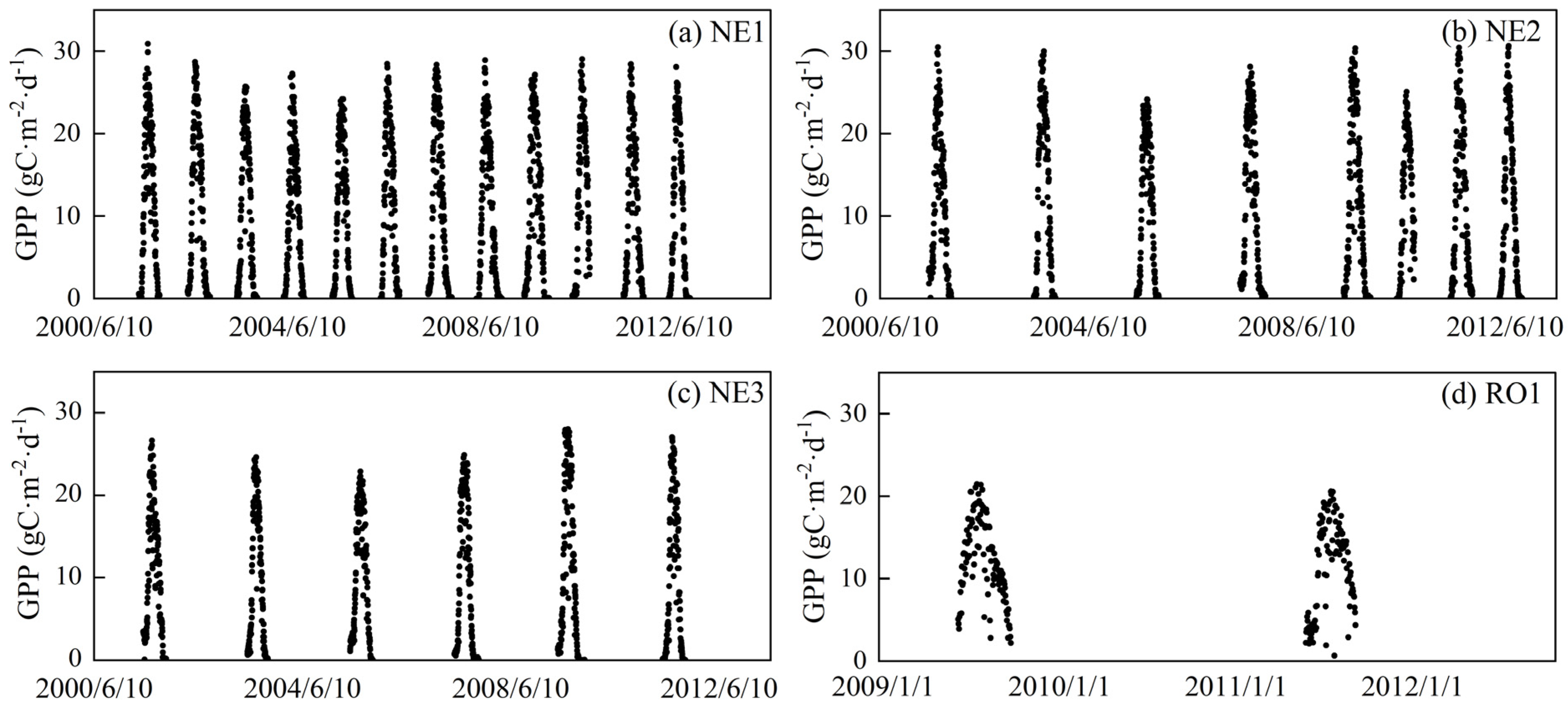
The data set of the RO1, NE1, NE2, and NE3 sites from Fluxnet 2015 provides hourly Tair, net ecosystem exchange (NEE), ecosystem respiration (Re), and SSR. The daily mean, minimum, and maximum Tair (i.e., Tmean, Tmin, and Tmax, respectively); NEE; and Re were computed based on hourly data. GPP was defined by NEE subtracting Re. The emergence and harvest days of three NE sites were obtained from the Carbon Sequestration Project (CSP) of the University of Nebraska (http://csp.unl.edu/public/, accessed on 10 March 2019). The start of season (SOS) and end of season (EOS) of the RO1 site were defined by Zhang et al. [50] with the reconstructed daily NDVI time series by Zeng et al. [51]. Consequently, the NE1, NE2, NE3, and RO1 sites have data availability for 1945, 1276, 987, and 214 days, respectively (Table 1). GPP ranges for four sites are presented in Figure 2.

2.2.2. Specific Leaf Nitrogen (SLN)

SLN (gN·m−2(leaf)) is defined as the nitrogen content per unit leaf area [38]. Ground-measured leaf mass per unit leaf area (LMA, gC·m−2), foliage nitrogen content (FNC, gN·100 g−1) and foliage carbon content (FCC, gC·100 g−1) at different phenological stages in the NE1, NE2, NE3 sites were obtained from the Carbon Sequestration Project (CSP) of the University of Nebraska (http://csp.unl.edu/public/, accessed on 10 March 2019). Then, SLN was calculated through the formula of SLN = LMA × FNC/FCC. The SLN data for the RO1 site were retrieved using multiple linear relationships established between maize phenology and SLN, which were trained using NE1, NE2, and NE3 data (details in Section 2.4). In the NE1, NE2, and NE3 sites, crop management practices (i.e., plant populations, herbicide and pesticide applications, irrigation) have been employed in accordance with standard best management practices (BMPs) for production-scale maize systems. To account for differences in water-limited attainable yield, plant densities were lower in rainfed crops at the NE3 site than in irrigated crops at the NE1 and NE2 sites. Total N fertilizer rates for both the irrigated and rainfed sites were adjusted for residual nitrate measured in soil samples taken each spring before planting following recommended guidelines (http://csp.unl.edu/public/sites.htm, accessed on 10 March 2019). Therefore, it can be inferred that there was hardly any fertilizer stress in the NE1, NE2, and NE3 sites. The computed SLN based on LMA, FNC, and FCC can be a proxy for the maximum allowable value.

2.3. Remotely Sensed NDVI

Daily NDVI, computed by (ρnir − ρred)/(ρnir + ρred), was applied in this study. ρnir and ρred are the spectral reflectances of near-infrared and red bands, respectively. MODIS MOD09GA and MOD09Q1 products downloaded via the Google Earth Engine (GEE) platform [52] provided daily and 8-day composite spectral reflectances of these two bands with a 250 m spatial resolution, respectively. Considering that directly computed NDVIs from the original daily product have a low data quality and those from 8-day composite product have a low temporal resolution, the DAVIR-MUTCOP method [53] was utilized to reconstruct daily NDVI time series combining the MODIS daily and 8-day composite products. It has been demonstrated that the DAVIR-MUTCOP method can effectively reconstruct daily NDVI time series of varied land cover types, particularly for cropland [53]. The reason why MODIS NDVI data were selected was based on the fact that the ground-measured data in three NE sites, especially for the maize GPP and SLN measurements, were only available before 2012. Before 2012, other satellites like Landsat are hard to use to provide reliable daily NDVI time series considering their low temporal resolution (16 days for Landsat), although they can provide NDVI data with high spatial resolution (30 m for Landsat). Additionally, satellites like Sentinel 2 can provide NDVI data with both acceptable temporal and spatial resolutions (5~10 day and 10 m), but they only obtain global NDVI data after 2016.

2.4. Relationship between Phenology and the Maximum Allowable SLN

Due to the big gap between satellite pixels (sub- to thousand-meter level) and plant leaves (up to decimeter level), it is hard to directly retrieve SLN by satellite remote sensing [54,55]. Previous studies have demonstrated that the maximum allowable SLN is a function of crop phenology [43,56], which is the base for simulating leaf nitrogen in several crop models, such as DSSAT-CERES [57], APSIM-Maize [58,59], SWAP, and WOFOST [60]. This provides a way to obtain SLN information after crop phenology is quantified. For maize, the temperature plays a crucial role in controlling phenological development [61,62]. The W-E model (Equations (1)–(4)) [63] was adopted to describe phenological development with daily mean air temperature data. To define the start of season (SOS) and the end of season (EOS) of maize, the method proposed by Zhang et al. [50] was used with the reconstructed NDVI time series data. Considering that photoperiod and soil conditions (e.g., water status) may change the phenological stage which completely relies on the temperature [64,65], a normalized maize phenological development factor of NMP (Equation (5)) was finally utilized to reflect maize’s phenological development.
f T = 2 ( T T b a s e ) α ( T o p t T b a s e ) α ( T T b a s e ) 2 α ( T o p t T b a s e ) 2 α ,   T b a s e T T u p
f T = 0 ,   T > T u p   o r   T < T b a s e
α = l n 2 l n [ ( T u p T b a s e ) / ( T o p t T b a s e ) ]
P D t = s o s t f T d t
N M P t = P D t / P D E O S
where t is the growing date; T is the daily mean air temperature; Tbase, Topt, and Tup are the minimum, optimal, and maximum temperature for maize growth, respectively, and assumed as 8 °C, 28 °C, and 36 °C, respectively [66].
The NMP and SLN data from the NE1, NE2, and NE3 sites were used to establish the statistical function between NMP and SLN. Subsequently, the SLN data of the RO1 site was derived by applying the established function after NMP was obtained using Equations (1)–(5).

2.5. Methodology

2.5.1. ML Methods

Four ML methods, including random forest (RF), support vector machine (SVM), convolutional neutral network (CNN), and extreme learning machine (ELM), were applied and compared in this study.
RF [67] is a machine learning algorithm that introduces randomness based on bagging ensemble learning [68]. It is widely used in the GPP estimation field [69,70,71]. The bootstrap method [72] is adopted to randomly and repeatedly extract training sample sets to form a forest containing m decision trees, thus producing m different results. The result of the final model is determined according to the voting method. The samples that are not extracted are called out-of-bag data, which are used to calculate out-of-bag error (OOB) and evaluate the model’s generalization ability. The generalization error of an RF model comes to reach the minimum as the number of trees increase. RF is also able to rank the importance of model input variables. As the importance value increases, the input variable has a greater impact on the output.
SVM is a tool for multi-dimensional function estimation and widely used in regression and classification [73,74,75]. Its principle is to map an input vector to a high-dimensional space to transform nonlinear regression into linear regression. Its superior generalization ability compared to traditional statistical methods [76] may make it more feasible to achieve satisfactory results in cross-site validation. This study chooses the penalty factor (c) and the parameter of radial basis kernel function (g) as the model parameters to set up the model.
CNN is a deep learning algorithm composed of input, convolutional, pooling, and fully connected layers [77]. The convolutional layer contains multiple convolutional kernels: a one-dimensional (1-D) convolutional kernel is used for ordinal data such as time series data, a 2-D convolutional kernel is used for images, and a 3-D kernel is used for video and 3D images. CNN’s hierarchical structure gives it the flexibility and applicability for a variety of complex regression tasks [78]. Compared to ANN, CNN demonstrates quicker learning of complex problems through weight sharing, enabling greater parallelization [79]. However, the accuracy of CNN’s learning relies on a large amount of data, often in the hundreds or thousands of data points. Fortunately, we have enough training data (N = 4208) to make up for that.
ELM is a new type of feedforward neutral network algorithm, consisting of input, hidden, and output layers [80]. The connection weight between the input layer and the hidden layer as well as the neuronal threshold value of the hidden layer are not adjusted after setting. To optimize the model, just the number of neurons in the hidden layer and the activation function need to be adjusted. Additionally, ELM converges significantly faster than traditional algorithms because there is no need for iterative learning [81]. In comparison to traditional networks requiring training all parameters, ELM simplifies the attainment of a global optimal solution using random parameters [81].

2.5.2. Input Variable Combinations

Vegetation photosynthesis is regulated by the soil, the atmosphere, and plant physiology. At the vegetation canopy scale, vegetation photosynthesis is closely related to solar radiation, air temperature, and nitrogen validity [82]. In the ecosystem level, vegetation photosynthesis is affected by climate, making the plant form different phenological stages. VIs can greatly reflect the canopy characteristics of vegetation and thus are widely used in models to estimate GPP. Based on previous research [27,74,83,84], NDVI, Tmean, Tmin, Tmax, SSR, SLN, and NMP were selected as input variables. Different input combinations were considered to evaluate the importance of input variables (Table 2). SLN and NMP characterizing the physiology of vegetation were introduced in ML models (A1, A2, A3) with the aim of enhancing model performance in contrast to existing studies. In this study, A1 and A2 aimed to test if individually considering SLN or NMP positively affected maize GPP prediction. A3, considering both SLN and NMP together, was utilized to compare with A1 and A2. A3 aimed to explore how including NMP when SLN was already an input (A1) or considering SLN when NMP was already an input (A2) impacts model accuracy. It also assessed whether combining both inputs enhances or reduces the accuracy of the original model (A0).

2.5.3. The Importance of SLN and NMP

The importance of all input variables was determined using the RF method based on the combination of A3. Additionally, to further verify the importance of NMP and SLN in the ML model, A0 and A3 were used for a comparison to evaluate the effectiveness based on the RF method from site to site. The NE1, NE2, and NE3 sites are in close proximity to each other, but they vary in terms of data size and moisture conditions. All data from three sites were selected to verify the role of SLN and NMP. The three sites are separated, and site-to-site verification is chosen between adjacent sites. The purpose is to evaluate whether the role of SLN and NMP is still maintained despite such differences. Three scenarios were set up for verification as follows:
(1)
NE1 for training and NE2 for testing: these two sites exhibit similar moisture levels, yet possess varying data quantities, and the larger data set is utilized to validate the smaller data set.
(2)
NE1 for training and NE3 for testing: the water conditions at the two sites differ, and the smaller data set is validated using the larger data set.
(3)
NE3 for training and NE2 for testing: due to the varying water conditions at the two sites, the smaller data set is employed to validate the larger data set.

2.5.4. Comparison of Different ML Methods

First, the selected four ML methods were trained and tested with the data from the NE1, NE2, and NE3 sites. A comparison of input variable combinations was conducted: 70% of data at three NE sites are randomly selected as the training set and the other 30% as the testing set, and this process runs 1000 times. Then, in order to evaluate ML’s robustness, the trained models based on the data from all three NE sites were further tested using the data from the RO1 site. For the other three ML methods (SVM, CNN, and ELM), A0 was also chosen as the control combination. When adding SLN and NMP (A1, A2, A3), a combination was selected for each ML method that results in the highest model accuracy during training and testing in three NE sites for RO1 validation. As a result, each ML method has two combinations of input variables for validation at the RO1 site.

2.6. Evaluation Metrics

Nash efficiency coefficient (NSE, Equation (6)), root mean square error (RMSE, Equation (7)), bias (Equation (8)), coefficient of variation (CV, Equation (9)), unbiased RMSE (URMSE, Equation (10)), and the slope of the fitting line between ground-measured and estimated GPP were used to evaluate different models’ performance. The closer NSE and slope are to one, and the closer RMSE, Bias, CV, and URMSE are to zero, the better the performance of the model.
N S E = 1 i = 1 n ( y m , i y g , i ) 2 ( y m , i y g , i ¯ ) 2
R M S E = i = 1 n ( y m , i y g , i ) 2 n 1
B i a s = i = 1 n ( y m , i y g , i ) n
C V = n × R M S E i = 1 n y g , i
U R M S E = R M S E 2 B i a s 2
where ym,i and yg,i are, respectively, the estimated and ground-measured GPP values of i model, and n is data size.
A list of acronyms and the corresponding explanations for input variables, ML methods, and evaluation metrics are presented in Appendix A.

3. Results

3.1. Relationship between Phenology and the Maximum Allowable SLN

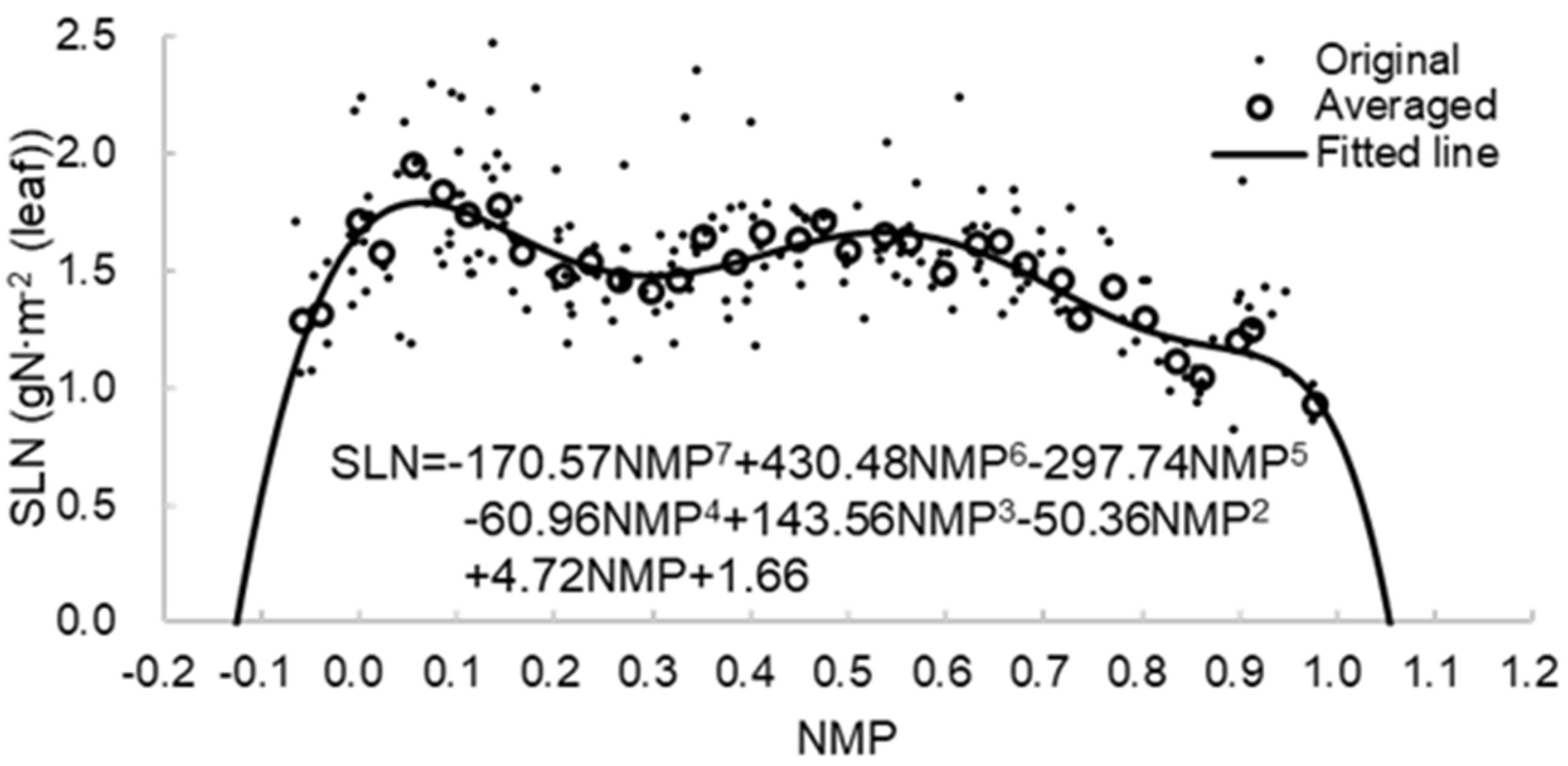
After maize’s phenological development represented by NMP was obtained using Equations (1)–(5), a polynomial function was applied to quantitatively construct the relationship between SLN and NMP based on the ground-measured data from the NE1, NE2, and NE3 sites (Figure 3). The curve shape of the fitting line in Figure 3 is consistent with the set in crop models, for example, the WOFOST maize crop model [60]. By controlling the same fitting parameters in Figure 3, the polynomial function was also used for the RO1 site.

3.2. Comparison of Input Variable Combinations Based on RF

3.2.1. RF Model Calibration and Input Variable Importance

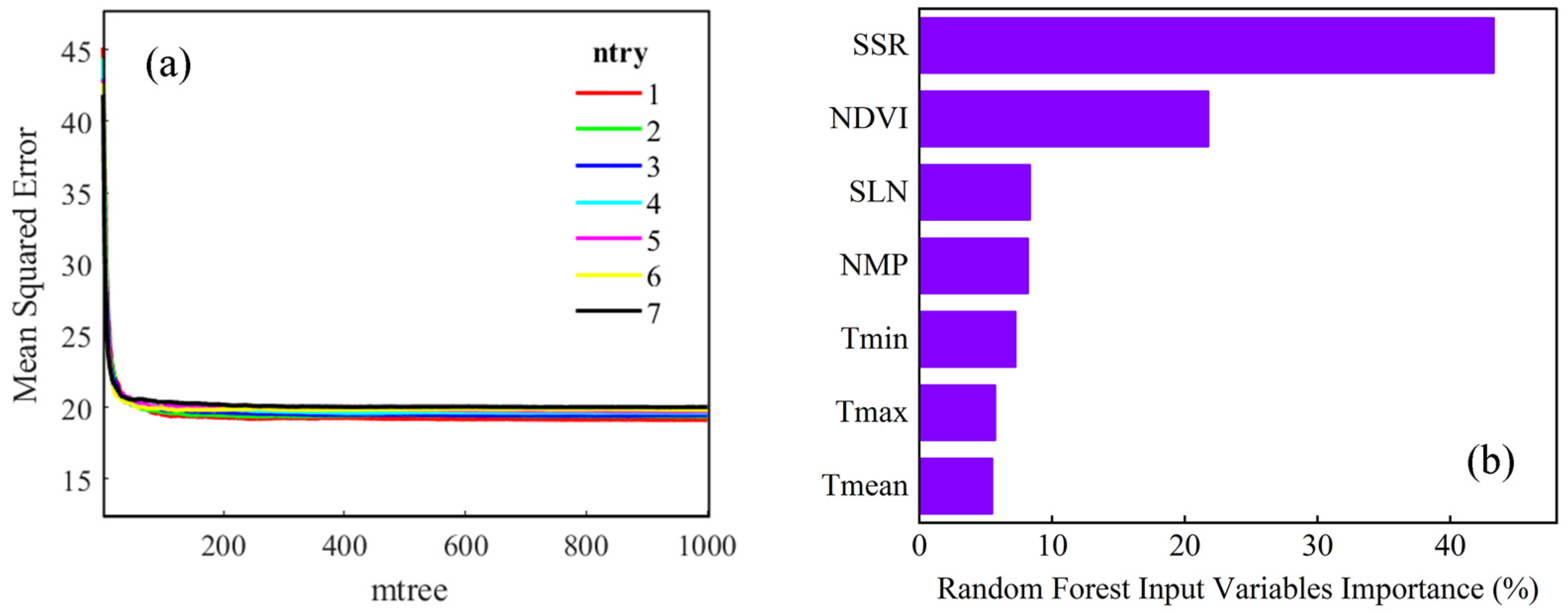
Data from the NE1, NE2, and NE3 sites were used to decide two parameters of RF (mtree: the number of decision trees; ntry: the number of preselected variables for a tree) considering NDVI, SSR, Tmin, Tmax, Tmean, SLN, and NMP as inputs. The gradient of mtree is set to 0~1000, and ntry is set to 1, 2, 3, 4, 5, 6, and 7, respectively. The out-of-bag error was characterized by mean square error (Figure 4).
From Figure 4a, as mtree increased, the model became more stable, but the computation time also increased. Thus, mtree was set to be 500. MSE had a low value when ntry was set to be 1~3. Considering that seven variables were included in total and based on a previous study [85], ntry was set to be 3. Figure 4b illustrates the importance ranking of input variables in the RF model when mtree = 500 and ntry = 3. SSR played the most critical role, accounting for about 43.3% of the total importance. This is easy to understand since SSR is the energy source for plant photosynthesis. The second was NDVI, whose proportion was 21.8%. The time series of NDVI effectively captures the changes in vegetation growth during various phenological stages [86]. Although temperature affects vegetation growth by controlling processes such as phenological development and enzyme activity [87], three kinds of temperature (i.e., Tmin, Tmax and Tmean) showed the weakest role, only accounting for 8.2%, 5.7%, and 5.5%, respectively. Interestingly, SLN and NMP also were proved to have considerable effects on the RF model, and their proportions were greater than the air temperature. As Figure 4b illustrates, these two factors played key roles in GPP estimation.

3.2.2. RF Performance in NE1, NE2, and NE3 Sites with Different Input Variable Combinations

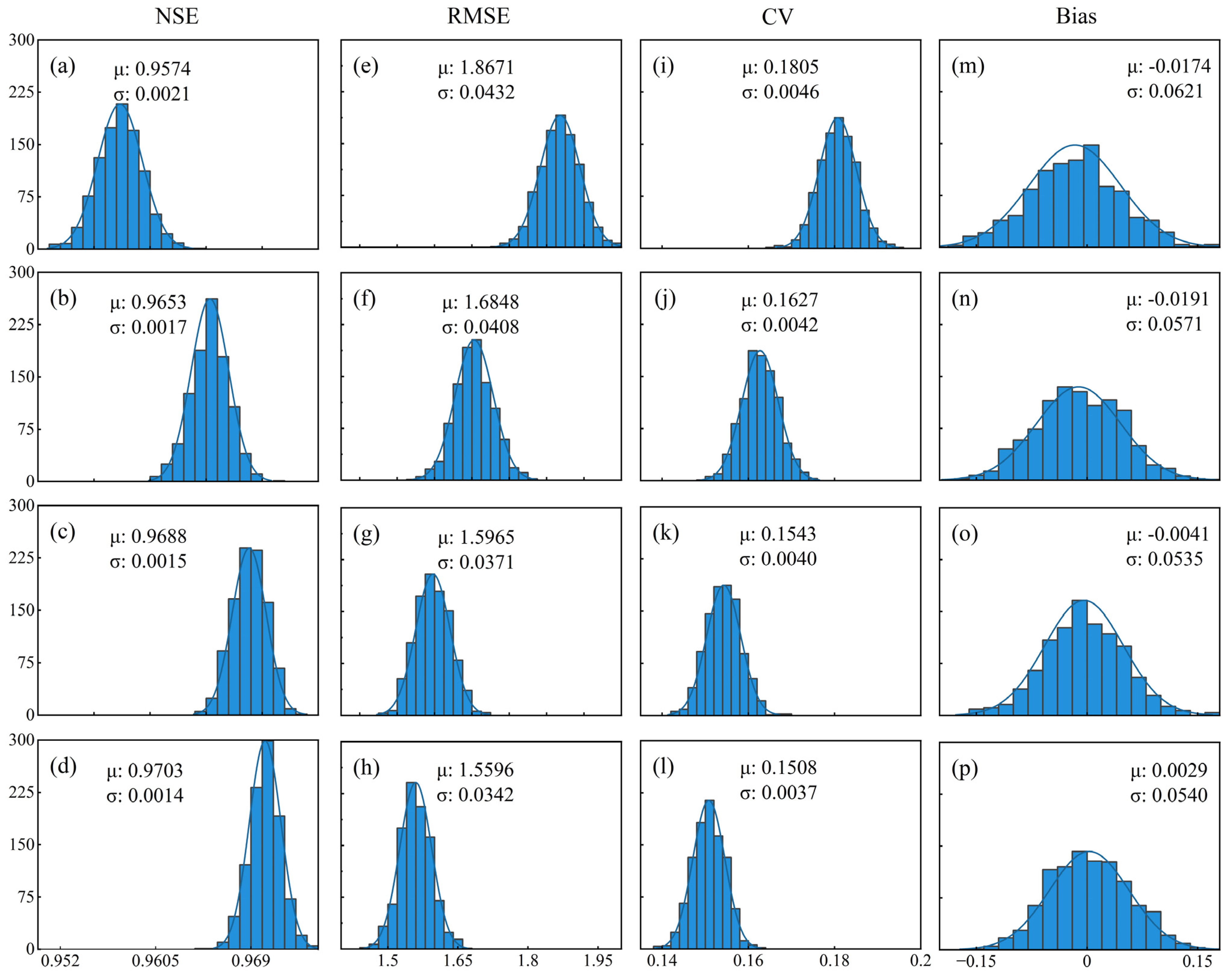
Input variable combinations in Table 2 were applied to test the performance of the RF model (mtree = 500, ntry = 3) in three NE sites (70% of data for training, and the other 30% for testing with random selection) by running it 1000 times. The test results are shown in Figure 5. In terms of mean value for comparison, A0 had the lowest accuracy (NSE = 0.9574, RMSE = 1.8671 gC·m−2·day−1, Bias = −0.0174 gC·m−2·day−1, CV = 0.1805). In contrast, when SLN and NMP alone or their combination were added as model inputs, the distribution plot of NSE gradually moved to the right side while the plots of RMSE and CV shifted to the left side with lower uncertainty. A3 obtained the highest accuracy (NSE = 0.9703, RMSE = 1.5596 gC·m−2·day−1, Bias = 0.0029 gC·m−2·day−1, CV = 0.1508). Thus, owing to the direct influence of SLN and NMP on carbon fixation such as maize leaf’s photosynthetic rate, they both boosted the performance of models.
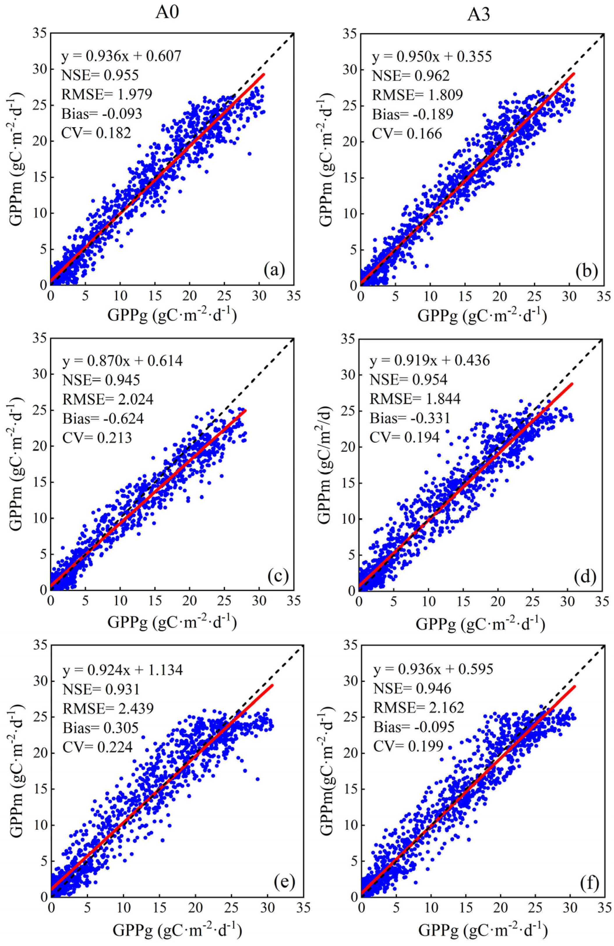
Data combinations of A0 and A3 (the minimum and maximum in Figure 5) were selected to further validate the effectiveness of NMP and SLN for RF among three NE sites (one site for training with another site for testing, as described in Section 2.5.3). In Figure 6, the estimated value was close to the ground-measured value when NMP and SLN were introduced in the model, whether for the NE1, NE2, or NE3 sites. They had higher NSE and lower RMSE and CV values. Moreover, the slope of the fitting line was closer to 1, and the intercept was closer to 0. In terms of NSE, RMSE, and CV, Figure 6a had the best model performance, as both NE1 and NE2 sites were contiguous and irrigated maize cropland and had similar growing environments. Figure 6e,f demonstrates the lowest accuracy in performance for A0 and A3 combinations, primarily due to the difference in growing environments (e.g., soil moisture) between the rainfed NE3 site and the irrigated NE2 site. Another contributing factor to the weak correlation in Figure 6e is the relatively small sample size for the NE3 site with a narrow GPP range (N = 987), making it difficult to accurately estimate GPP for the NE1 site with a wide GPP range (N = 1945).

3.2.3. RF Performance in RO1 Site While Trained in NE1, NE2, and NE3 Sites

RF performance was further validated in the RO1 site by training it with all data from the three NE sites (mtree = 500 and ntry = 3). The growing environments, including soil texture and moisture, weather, etc., were significantly different between the RO1 site and the three NE sites. It will further demonstrate whether the RF method trained by three NE sites could maintain the effectiveness when it was applied to other unknown sites. The validation results of four input variable combinations (Table 2) are shown in Figure 7. Although the estimated GPP of all combinations had a good linear relationship with ground-measured GPP (slope = 1.008~1.070 and NSE = 0.709~0.758), they showed a slight overestimation of GPP for the RO1 site (Bias = 0.609~1.464). Ground-measured GPP values of the three NE sites ranged from 0 to 33 gC·m−2·day−1 while ground-measured GPP values of the RO1 site ranged only between 0 and 22 gC·m−2·day−1. The maximum GPP value in the NE sites was higher than that in the RO1 site. This might be the reason why the estimated GPP of the RO1 site tended to be overestimated when GPP data from the three NE sites were used for model training. In Figure 7, it can be seen that SLN and NMP have boosted the model precision in terms of NSE, RMSE, and CV. Therefore, the RF method considering SLN and NMP had potential for an unknown site’s GPP estimation. However, it was noted that the results of both the A1 and A2 combinations were superior than that of the A3 combination, particularly for the A2 combination. It was speculated that there was redundancy in input data considering the explicit polynomial function between SLN and NMP (Figure 3).

3.3. Comparison of Different ML Model Performances

3.3.1. Comparison of Model Performance in NE1, NE2, and NE3 Sites

With 70% of data in the NE1, NE2, and NE3 sites as the training set and the other 30% as the testing set, three other ML methods (i.e., SVM, CNN and ELM) also completed 1000 random runs. The parameters of the SVM model were determined by the grid search and cross-validation approaches [88] (c = 16, g = 1). The parameters of the CNN model were determined by the stochastic gradient descent with momentum (SGDM) algorithm (max epochs = 1000, mini batchsize = 1200, initial learn rate = 0.01, learn rate drop factor = 0.5). A 3 × 1 convolution kernel was used in the CNN model. An appropriate activation function was the key factor to promote arithmetic speed for the ELM model, and a sigmoid activation function was adopted for calculation (number of hidden layer nodes = 50). In Table 3, the performance of all four ML methods is shown to be strong for estimating maize’s daily GPP. The SVM was the best, and the evaluation metrics of NSE, RMSE, and CV were improved compared with that of RF. CNN had the weakest performance, but its accuracy was very close to other ML methods. It has also demonstrated that the performance of all models significantly improved when SLN or NMP was introduced, although various ML methods showed different sensitivity to them. As for RF and SVM, model performance was better when SLN and NMP were considered simultaneously. But for CNN and ELM, NMP had a stronger ability than SLN for model improvement. It was speculated that the data redundancy in the input variables of SLN and NMP with a fixed polynomial relationship led to this result. Combining Figure 7 and Table 3, the CNN and ELM methods might be more sensitive to data redundancy than the RF and SVM methods.

3.3.2. Comparison of Model Performances in RO1 Site

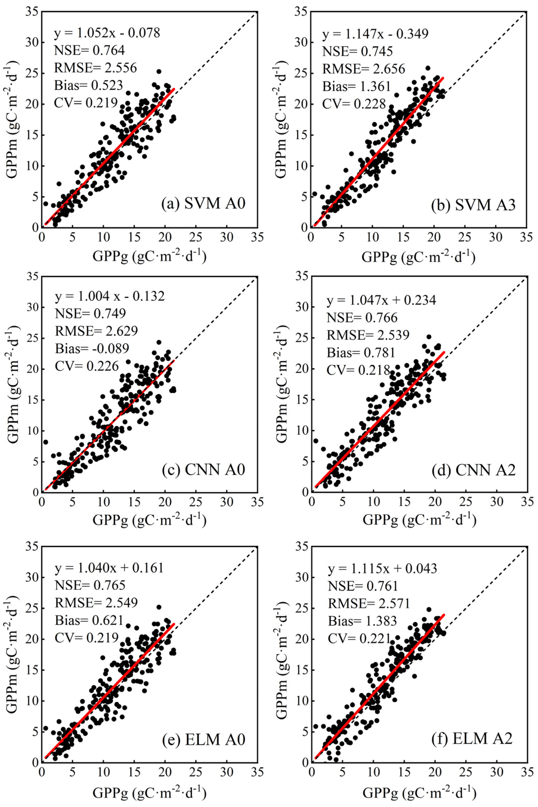
Based on the results of Section 3.3.1, optimal input variable combinations (bolded font in Table 3) were selected for four ML methods to validate the model performance using the RO1 site, while data from three NE sites were used for training. The input variable combination of A0 was considered the control combination. The ML methods provided accurate estimates for GPP in the RO1 site, providing sufficient evidence of successful parameter settings in Section 3.3.1 and ensuring the adequate generalization of the model (Figure 7 for RF and Figure 8 for SVM, CNN, and ELM). The slope was close to 1 and the intercept was close to 0. The URMSE was also computed and applied to further analyze the effect of SLN and NMP on each of the models. The ELM model performed best (NSE = 0.765, RMSE = 2.549 gC·m−2·day−1, Bias = 0.621 gC·m−2·day−1 and CV = 0.219), and the performance of the SVM model was rated as the second best (NSE = 0.764, RMSE = 2.556 gC·m−2·day−1, Bias = 0.523 gC·m−2·day−1 and CV = 0.219) when the variables SLN and NMP were not taken into account (A0 combination). Despite the integration of SLN and NMP leading to reduced accuracy in both SVM and ELM, as shown by the evaluation metrics in Figure 8, the decline is not substantial. Additionally, Figure 8b,d demonstrate that data points are more tightly clustered to the fitting line. In addition, in Table 4, it could be also concluded that not all URMSEs of each model varied consistently with RMSE. For both SVM and ELM, their URMSE decreased with the increase in RMSE. Thus, the effectiveness of the SVM and ELM algorithms was still evident for site-to-site validation. The consideration of NMP brought CNN the best accuracy (NSE = 0.766, RMSE = 2.539 gC·m−2·day−1, Bias = 0.781 gC·m−2·day−1 and CV = 0.218), and its URMSE also decreased. The accuracy of RF significantly increased when considering SLN and NMP simultaneously, as shown in Figure 7d, with its URMSE reaching the second lowest level. Moreover, all URMSE values decreased compared to the RMSE, and ELM had the lowest URMSE. Therefore, one the one hand, based on the NSE, RMSE, and CV, the additional input variables of SLN and NMP supported the RF and CNN algorithms in enhancing the accuracy. One the other hand, according to the URMSE, all the ML models maintained robustness with the supplement of SLN and NMP.

4. Discussion

In this study, four ML methods were used to predict the maize GPP of three sites in Nebraska (i.e., the NE1, NE2, and NE3 sites) and one site in Minnesota (i.e., the RO1 site). Previous ML models simply took processed meteorological data and remote sensing data as model inputs, without the consideration of influences from phenology and leaf physiology on photosynthesis. The novelty of this study is integrating maize phenology (represented by NMP) and leaf photosynthetic rate factor determined by phenology (represented by SLN) into the model inputs. The selection of appropriate input variables plays a key role in GPP prediction [89]. The contribution rate of selected variables and the importance of SLN and NMP are further verified by ranking the importance of input factors in the RF method. SSR is the most important contribution factor (43.3%) to GPP, and it is the main energy source of organisms. There is a direct relationship between photosynthesis and SSR. The physiological process and photosynthesis of maize are regulated by the light and thermal effects brought by radiation [90]. The contribution rate of NDVI is 21.8%, and it is the most commonly used feature factor, which can reflect the plant canopy dynamics. The greater the amount of green vegetation, the more infrared light it absorbs, leading to a rise in NDVI [91]. Unexpectedly, the contribution of SLN and NMP factors exceeded that of air temperature, suggesting that they also had a significant impact on GPP estimates. Three kinds of temperature also have a certain proportion, reflecting the characteristics of the climate of the site. In addition, by regulating the physiological process of vegetation, temperature makes it form a phenological process for maize to a large extent. Therefore, there is a certain correlation between temperature and phenological factor (NMP). But by using data from three NE sites in Nebraska, the four ML methods all prove that the positive effect of NMP on the model (A3) can compensate for the decrease in accuracy caused by information overlap. Therefore, it is feasible to consider the three temperature and NMP factors simultaneously.
The role of SLN and NMP were further validated from site to site in Nebraska using the RF method. The division of the training set and test set was determined by the respective data volume and water stress differences of the three sites, and the optimal input variable combination of Section 3.2.2 was used. SLN and NMP both maintained their positive impact on the model, but to different degrees, depending on the specific soil and water information at each site. When the other three ML methods (SVM, CNN, and ELM) were applied to GPP prediction for all three sites in Nebraska, good results were also obtained (NSE > 0.95 and RMSE < 2 gC·m−2·day−1), and the estimation accuracy of all methods was similar. Specifically, after considering SLN and NMP, the accuracy of all models improved. But when SLN and NMP were considered at the same time, SVM and RF had the greatest improvement, while for CNN and ELM, only when SLN or NMP was considered separately. CNN uses a more complex model and weight sharing in its algorithm, which can learn complex problems quickly. BP neural network algorithms use single hidden layer feedforward neural networks (SLFNs) as universal approximators, but their parameter optimization is complicated [92]. ELM just solves this problem, and its hidden layer parameters do not need to be optimized. At the same time, the approximation capability of SLFNs can be maintained. Therefore, the correlation between SLN and NMP created an overlap of known information in CNN and ELM. Thus, the accuracy of CNN and ELM decreased, so it was better to use only one kind of physiological information. In the verification using the RO1 site, the addition of SLN and NMP enabled different ML methods to obtain different results using the unbiased estimator (URMSE) for evaluation. All ML methods had a high degree of fit of scatter points after considering physiological information, which proved its effectiveness.
In the process of evaluating the accuracy of GPP prediction results, data uncertainty has impacts on the verification of results. First, inaccurate GPP observations in flux towers will produce errors [75], and there are uncertainties in NDVI remote sensing observation data sources. The GPP at three Nebraska sites ranges from 0 and 32 gC·m−2·day−1, which leads to the saturation of NDVI [93]. The reconstruction of NDVI using a 8-day MOD09Q1 product and a daily MOD09Q1 product can generally obtain higher accuracy. However, in cloudy conditions, the 8-day composite product still contains continuous noise [53]. Secondly, the maximum allowable SLN we considered was obtained at leaf scale, which has the problem of scale mismatch with meteorological data and remote sensing data. Moreover, the SLN of the RO1 site was derived from the polynomial fitting relationship between NMP and SLN at three sites in Nebraska, and the points in Figure 3 are still discrete to some extent, which also brings uncertainty. Thirdly, when RO1 was used for verification, all models produced a high RMSE, which was probably due to the differences in farmland management between the RO1 site and the three sites in Nebraska. Differences in moisture and soil brought about spatial consistency. Finally, ML method sensitivity is highly dependent on the amount of data and its accuracy [94]. While the data set used in this study has high accuracy, errors in the training data set and correlations between input variables (such as SLN and NMP) can affect GPP estimation.
Through the results, the advantages of SLN and NMP in improving maize daily GPP estimation via four ML methods have been demonstrated. In the future, it would be interesting to consider other vegetation indices in the input to correct the saturation phenomenon of NDVI in high-value GPP. Moreover, certain important factors associated with site meteorological data, such as vapor pressure deficit (VPD) and soil moisture, are anticipated to be incorporated into the model. In addition, utilizing longer time spans of data to increase data volume to enhance data alignment is another method to enhance accuracy. Note that, owing to the fixed polynomial function between SLN and NMP, data redundancy seemed to occur. On the one hand, in this case, the introduction of SLN or NMP alone, rather than both, may guarantee the robustness of ML methods, such as ELM and CNN (Table 3). On the other hand, direct measurement or high-frequency remote sensing inversion of SLN is needed in the future to further study the value of SLN. However, the big gap between satellite pixel and leaf blade areas will make it a big challenge for SLN inversion via satellite platforms. Fortunately, low-altitude unmanned aerial vehicles (UAVs) provide an available way at the regional scale.

5. Conclusions

GPP plays key role in maintaining carbon balance in terrestrial ecosystems and climate change. It is essential to accurately quantify daily GPP. This study, taking maize as an example, based on five traditional inputs (NDVI, SSR, Tmean, Tmin, and Tmax), we discussed the importance of NMP and SLN in improving the daily GPP estimation via four popular ML methods (RF, SVM, CNN, and ELM). The prediction results are assessed in detail and comprehensively compared using accuracy metrics (NSE, RMSE, Bias, CV, and URMSE).
The advantages of introducing NMP and SLN into inputs have been demonstrated by all applied ML methods with the flux data in four sites. It is just that different ML methods have different sensitivities to SLN and NMP. The significance of SLN and NMP was also confirmed in the importance ranking of random forest. It is noted that considering the fixed relationship between the maximum allowable SLN and NMP, for the CNN and ELM methods, introducing NMP or SLN alone may obtain superior results than introducing them simultaneously. This study indicates that plant phenology and leaf-level photosynthetic factors have great value in improving GPP estimation via ML methods. But they have been commonly ignored by previous research. ML methods with the consideration of SLN or NMP are expected to improve the evaluation accuracy of global maize GPP.
All in all, as organic matter accumulates via maize photosynthesis, GPP exhibits a direct correlation with photosynthesis rate. SLN and NMP, concurrently regulating photosynthesis, exert an influence on GPP synthesis. Integrating these dynamic physiological aspects of maize as input variables into machine learning models has notably improved the models’ accuracy. This study provided new insights to improve GPP estimation via ML methods.

Author Contributions

C.H.: methodology, software, validation, formal analysis, data curation, writing—original draft preparation; S.H.: conceptualization, methodology, validation, formal analysis, data curation, investigation, data curation, writing—review and editing, supervision, project administration, funding acquisition; L.Z.: formal analysis, writing—review and editing; K.M.: writing—review and editing; Z.L.: project administration, writing—review and editing; K.W.: writing—review and editing. All authors have read and agreed to the published version of the manuscript.

Funding

This work was supported by the National Nature Science Foundation of China program (Grant No. 42207098), Yinshanbeilu Grassland Eco-hydrology National Observation and Research Station, China Institute of Water Resources and Hydropower Research (Grant No. YSS202302).

Data Availability Statement

The data are available from the corresponding author on reasonable request. The data are not publicly available due to that there are still graduate students using it for research.

Conflicts of Interest

The authors declare no conflicts of interest.

Appendix A

Table A1. Acronyms and the corresponding explanations of input variables.
AcronymFull NameUnitsSource
TmeanDaily mean air temperature°CFLUXNET 2015
TminDaily minimum air temperature°CFLUXNET 2015
TmaxDaily maximum air temperature°CFLUXNET 2015
SSRSolar shortwave radiationMJ·m−2·day−1FLUXNET 2015
NDVINormalized difference vegetation index-MOD09GQ, MOD09Q1
SLNSpecific leaf nitrogengN·m−2(leaf)CSP of the University of Nebraska
NMPNormalized maize phenology-Wang-Engel model [64]
Table A2. Acronyms and the corresponding full name of machine learning (ML) methods (RF, SVM, CNN, and ELM) and the model evaluation metrics (NSE, RMSE, CV, and URMSE).
AcronymFull Name
RFRandom forest
SVMSupport vector machine
CNNConvolutional neural network
ELMExtreme learning machine
NSENash efficiency coefficient (-)
RMSERoot mean square efficiency (gC·m−2·day−1)
CVCoefficient of variation (-)
URMSEUnbiased root mean square efficiency (gC·m−2·day−1)

References

  1. Wu, C.; Munger, J.W.; Niu, Z.; Kuang, D. Comparison of Multiple Models for Estimating Gross Primary Production Using MODIS and Eddy Covariance Data in Harvard Forest. Remote Sens. Environ. 2010, 114, 2925–2939. [Google Scholar] [CrossRef]
  2. Wang, M.; Wang, S.; Zhao, J.; Ju, W.; Hao, Z. Global Positive Gross Primary Productivity Extremes and Climate Contributions during 1982–2016. Sci. Total Environ. 2021, 774, 145703. [Google Scholar] [CrossRef]
  3. Field, C.B.; Behrenfeld, M.J.; Randerson, J.T.; Falkowski, P. Primary Production of the Biosphere: Integrating Terrestrial and Oceanic Components. Science 1998, 281, 237–240. [Google Scholar] [CrossRef] [PubMed]
  4. Gilabert, M.; Sánchez-Ruiz, S.; Moreno, Á. Annual Gross Primary Production from Vegetation Indices: A Theoretically Sound Approach. Remote Sens. 2017, 9, 193. [Google Scholar] [CrossRef]
  5. Ramankutty, N.; Evan, A.T.; Monfreda, C.; Foley, J.A. Farming the Planet: 1. Geographic Distribution of Global Agricultural Lands in the Year 2000: GLOBAL AGRICULTURAL LANDS IN 2000. Glob. Biogeochem. Cycles 2008, 22. [Google Scholar] [CrossRef]
  6. Chen, T.; Van Der Werf, G.R.; Gobron, N.; Moors, E.J.; Dolman, A.J. Global Cropland Monthly Gross Primary Production in the Year 2000. Biogeosciences 2014, 11, 3871–3880. [Google Scholar] [CrossRef]
  7. Beer, C.; Reichstein, M.; Tomelleri, E.; Ciais, P.; Jung, M.; Carvalhais, N.; Rödenbeck, C.; Arain, M.A.; Baldocchi, D.; Bonan, G.B. Terrestrial Gross Carbon Dioxide Uptake: Global Distribution and Covariation with Climate. Science 2010, 329, 834–838. [Google Scholar] [CrossRef]
  8. Sims, D.; Rahman, A.; Cordova, V.; Elmasri, B.; Baldocchi, D.; Bolstad, P.; Flanagan, L.; Goldstein, A.; Hollinger, D.; Misson, L. A New Model of Gross Primary Productivity for North American Ecosystems Based Solely on the Enhanced Vegetation Index and Land Surface Temperature from MODIS. Remote Sens. Environ. 2008, 112, 1633–1646. [Google Scholar] [CrossRef]
  9. Keenan, T.F.; Davidson, E.; Moffat, A.M.; Munger, W.; Richardson, A.D. Using Model-Data Fusion to Interpret Past Trends, and Quantify Uncertainties in Future Projections, of Terrestrial Ecosystem Carbon Cycling. Glob. Chang. Biol. 2012, 18, 2555–2569. [Google Scholar] [CrossRef]
  10. Zhu, A.X.; Scott Mackay, D. Effects of Spatial Detail of Soil Information on Watershed Modeling. J. Hydrol. 2001, 248, 54–77. [Google Scholar] [CrossRef]
  11. Running, S.W.; Nemani, R.R.; Heinsch, F.A.; Zhao, M.; Reeves, M.; Hashimoto, H. A Continuous Satellite-Derived Measure of Global Terrestrial Primary Production. BioScience 2004, 54, 547. [Google Scholar] [CrossRef]
  12. Gamon, J.A.; Serrano, L.; Surfus, J.S. The Photochemical Reflectance Index: An Optical Indicator of Photosynthetic Radiation Use Efficiency across Species, Functional Types, and Nutrient Levels. Oecologia 1997, 112, 492–501. [Google Scholar] [CrossRef] [PubMed]
  13. Suyker, A.E.; Verma, S.B. Gross Primary Production and Ecosystem Respiration of Irrigated and Rainfed Maize–Soybean Cropping Systems over 8 Years. Agric. For. Meteorol. 2012, 165, 12–24. [Google Scholar] [CrossRef]
  14. Xiao, X.; Zhang, Q.; Hollinger, D.; Aber, J.; Moore, B. Modeling Gross Primary Production of an Evergreen Needleleaf Forest Using Modis and Climate Data. Ecol. Appl. 2005, 15, 954–969. [Google Scholar] [CrossRef]
  15. Yuan, W.; Cai, W.; Nguy-Robertson, A.L.; Fang, H.; Suyker, A.E.; Chen, Y.; Dong, W.; Liu, S.; Zhang, H. Uncertainty in Simulating Gross Primary Production of Cropland Ecosystem from Satellite-Based Models. Agric. For. Meteorol. 2015, 207, 48–57. [Google Scholar] [CrossRef]
  16. Pettorelli, N.; Vik, J.O.; Mysterud, A.; Gaillard, J.-M.; Tucker, C.J.; Stenseth, N.C. Using the Satellite-Derived NDVI to Assess Ecological Responses to Environmental Change. Trends Ecol. Evol. 2005, 20, 503–510. [Google Scholar] [CrossRef] [PubMed]
  17. Crane-Droesch, A. Machine Learning Methods for Crop Yield Prediction and Climate Change Impact Assessment in Agriculture. Environ. Res. Lett. 2018, 13, 114003. [Google Scholar] [CrossRef]
  18. Veenadhari, S.; Misra, B.; Singh, C. Machine Learning Approach for Forecasting Crop Yield Based on Climatic Parameters. In Proceedings of the 2014 International Conference on Computer Communication and Informatics, Coimbatore, India, 3–5 January 2014; IEEE: Piscataway, NJ, USA, 2014; pp. 1–5. [Google Scholar]
  19. Palanivel, K.; Surianarayanan, C. An Approach for Prediction of Crop Yield Using Machine Learning and Big Data Techniques. Int. J. Comput. Eng. Technol. 2019, 10, 110–118. [Google Scholar] [CrossRef]
  20. Schlenker, W.; Roberts, M.J. Nonlinear Effects of Weather on Corn Yields. Rev. Agric. Econ. 2006, 28, 391–398. [Google Scholar] [CrossRef]
  21. Khaki, S.; Wang, L. Crop Yield Prediction Using Deep Neural Networks. Front. Plant Sci. 2019, 10, 621. [Google Scholar] [CrossRef]
  22. Benos, L.; Tagarakis, A.C.; Dolias, G.; Berruto, R.; Kateris, D.; Bochtis, D. Machine Learning in Agriculture: A Comprehensive Updated Review. Sensors 2021, 21, 3758. [Google Scholar] [CrossRef] [PubMed]
  23. Cutler, D.R.; Edwards, T.C.; Beard, K.H.; Cutler, A.; Hess, K.T.; Gibson, J.; Lawler, J.J. Random Forests for Classification in Ecology. Ecology 2007, 88, 2783–2792. [Google Scholar] [CrossRef] [PubMed]
  24. Bai, Y.; Liang, S.; Yuan, W. Estimating Global Gross Primary Production from Sun-Induced Chlorophyll Fluorescence Data and Auxiliary Information Using Machine Learning Methods. Remote Sens. 2021, 13, 963. [Google Scholar] [CrossRef]
  25. Dou, X.; Yang, Y. Comprehensive Evaluation of Machine Learning Techniques for Estimating the Responses of Carbon Fluxes to Climatic Forces in Different Terrestrial Ecosystems. Atmosphere 2018, 9, 83. [Google Scholar] [CrossRef]
  26. Mishra, S.; Mishra, D.; Santra, G.H. Applications of Machine Learning Techniques in Agricultural Crop Production: A Review Paper. Indian J. Sci. Technol. 2016, 9, 1–14. [Google Scholar] [CrossRef]
  27. Prakash Sarkar, D.; Uma Shankar, B.; Ranjan Parida, B. Machine Learning Approach to Predict Terrestrial Gross Primary Productivity Using Topographical and Remote Sensing Data. Ecol. Inform. 2022, 70, 101697. [Google Scholar] [CrossRef]
  28. Zhu, X.-J.; Yu, G.-R.; Chen, Z.; Zhang, W.-K.; Han, L.; Wang, Q.-F.; Chen, S.-P.; Liu, S.-M.; Wang, H.-M.; Yan, J.-H.; et al. Mapping Chinese Annual Gross Primary Productivity with Eddy Covariance Measurements and Machine Learning. Sci. Total Environ. 2023, 857, 159390. [Google Scholar] [CrossRef]
  29. Gu, L.; Post, W.M.; Baldocchi, D.; Andy Black, T.; Verma, S.B.; Vesala, T.; Wofsy, S.C. Phenology of Vegetation Photosynthesis. In Phenology: An Integrative Environmental Science; Schwartz, M.D., Ed.; Tasks for Vegetation Science; Springer: Dordrecht, The Netherlands, 2003; Volume 39, pp. 467–485. ISBN 978-1-4020-1580-9. [Google Scholar]
  30. Peñuelas, J.; Rutishauser, T.; Filella, I. Phenology Feedbacks on Climate Change. Science 2009, 324, 887–888. [Google Scholar] [CrossRef]
  31. Richardson, A.D.; Andy Black, T.; Ciais, P.; Delbart, N.; Friedl, M.A.; Gobron, N.; Hollinger, D.Y.; Kutsch, W.L.; Longdoz, B.; Luyssaert, S.; et al. Influence of Spring and Autumn Phenological Transitions on Forest Ecosystem Productivity. Phil. Trans. R. Soc. B 2010, 365, 3227–3246. [Google Scholar] [CrossRef]
  32. Croft, H.; Chen, J.M.; Luo, X.; Bartlett, P.; Chen, B.; Staebler, R.M. Leaf Chlorophyll Content as a Proxy for Leaf Photosynthetic Capacity. Glob. Chang. Biol. 2017, 23, 3513–3524. [Google Scholar] [CrossRef]
  33. Li, Y.; He, N.; Hou, J.; Xu, L.; Liu, C.; Zhang, J.; Wang, Q.; Zhang, X.; Wu, X. Factors Influencing Leaf Chlorophyll Content in Natural Forests at the Biome Scale. Front. Ecol. Evol. 2018, 6, 64. [Google Scholar] [CrossRef]
  34. Schlemmer, M.; Gitelson, A.; Schepers, J.; Ferguson, R.; Peng, Y.; Shanahan, J.; Rundquist, D. Remote Estimation of Nitrogen and Chlorophyll Contents in Maize at Leaf and Canopy Levels. Int. J. Appl. Earth Obs. Geoinf. 2013, 25, 47–54. [Google Scholar] [CrossRef]
  35. Gitelson, A.A. Novel Technique for Remote Estimation of CO2 Flux in Maize. Geophys. Res. Lett. 2003, 30, 1486. [Google Scholar] [CrossRef]
  36. Schepers, J.S.; Francis, D.D.; Vigil, M.; Below, F.E. Comparison of Corn Leaf Nitrogen Concentration and Chlorophyll Meter Readings. Commun. Soil Sci. Plant Anal. 1992, 23, 2173–2187. [Google Scholar] [CrossRef]
  37. Daughtry, C. Estimating Corn Leaf Chlorophyll Concentration from Leaf and Canopy Reflectance. Remote Sens. Environ. 2000, 74, 229–239. [Google Scholar] [CrossRef]
  38. Muchow, R.C.; Sinclair, T.R. Nitrogen Response of Leaf Photosynthesis and Canopy Radiation Use Efficiency in Field-Grown Maize and Sorghum. Crop Sci. 1994, 34, 721–727. [Google Scholar] [CrossRef]
  39. Allison, J.C.S.; Williams, H.T.; Pammenter, N.W. Effect of Specific Leaf Nitrogen Content on Photosynthesis of Sugarcane. Ann. Appl. Biol. 1997, 131, 339–350. [Google Scholar] [CrossRef]
  40. Houborg, R.; Cescatti, A.; Migliavacca, M.; Kustas, W.P. Satellite Retrievals of Leaf Chlorophyll and Photosynthetic Capacity for Improved Modeling of GPP. Agric. For. Meteorol. 2013, 177, 10–23. [Google Scholar] [CrossRef]
  41. Sinclair, T.R.; Horie, T. Leaf Nitrogen, Photosynthesis, and Crop Radiation Use Efficiency: A Review. Crop Sci. 1989, 29, 90–98. [Google Scholar] [CrossRef]
  42. Muchow, R.C. Effect of Nitrogen Supply on the Comparative Productivity of Maize and Sorghum in a Semi-Arid Tropical Environment I. Leaf Growth and Leaf Nitrogen. Field Crops Res. 1988, 18, 1–16. [Google Scholar] [CrossRef]
  43. Hammer, G.L.; Van Oosterom, E.; McLean, G.; Chapman, S.C.; Broad, I.; Harland, P.; Muchow, R.C. Adapting APSIM to Model the Physiology and Genetics of Complex Adaptive Traits in Field Crops. J. Exp. Bot. 2010, 61, 2185–2202. [Google Scholar] [CrossRef] [PubMed]
  44. Porter, J.R. AFRCWHEAT2: A Model of the Growth and Development of Wheat Incorporating Responses to Water and Nitrogen. Eur. J. Agron. 1993, 2, 69–82. [Google Scholar] [CrossRef]
  45. Wu, A.; Song, Y.; Van Oosterom, E.J.; Hammer, G.L. Connecting Biochemical Photosynthesis Models with Crop Models to Support Crop Improvement. Front. Plant Sci. 2016, 7, 1518. [Google Scholar] [CrossRef]
  46. Huang, X.; Xiao, J.; Ma, M. Evaluating the Performance of Satellite-Derived Vegetation Indices for Estimating Gross Primary Productivity Using FLUXNET Observations across the Globe. Remote Sens. 2019, 11, 1823. [Google Scholar] [CrossRef]
  47. Wang, J.; Dong, J.; Yi, Y.; Lu, G.; Oyler, J.; Smith, W.K.; Zhao, M.; Liu, J.; Running, S. Decreasing Net Primary Production Due to Drought and Slight Decreases in Solar Radiation in China from 2000 to 2012: Decreasing NPP Due To Solar Radiation. J. Geophys. Res. Biogeosci. 2017, 122, 261–278. [Google Scholar] [CrossRef]
  48. Liu, Y.; Ju, W.; He, H.; Wang, S.; Sun, R.; Zhang, Y. Changes of Net Primary Productivity in China during Recent 11 Years Detected Using an Ecological Model Driven by MODIS Data. Front. Earth Sci. 2013, 7, 112–127. [Google Scholar] [CrossRef]
  49. Verma, S.B.; Dobermann, A.; Cassman, K.G.; Walters, D.T.; Knops, J.M.; Arkebauer, T.J.; Suyker, A.E.; Burba, G.G.; Amos, B.; Yang, H.; et al. Annual Carbon Dioxide Exchange in Irrigated and Rainfed Maize-Based Agroecosystems. Agric. For. Meteorol. 2005, 131, 77–96. [Google Scholar] [CrossRef]
  50. Zhang, X.; Friedl, M.A.; Schaaf, C.B.; Strahler, A.H.; Hodges, J.C.F.; Gao, F.; Reed, B.C.; Huete, A. Monitoring Vegetation Phenology Using MODIS. Remote Sens. Environ. 2003, 84, 471–475. [Google Scholar] [CrossRef]
  51. Zeng, L.; Wardlow, B.D.; Wang, R.; Shan, J.; Tadesse, T.; Hayes, M.J.; Li, D. A Hybrid Approach for Detecting Corn and Soybean Phenology with Time-Series MODIS Data. Remote Sens. Environ. 2016, 181, 237–250. [Google Scholar] [CrossRef]
  52. Amani, M.; Ghorbanian, A.; Ahmadi, S.A.; Kakooei, M.; Moghimi, A.; Mirmazloumi, S.M.; Moghaddam, S.H.A.; Mahdavi, S.; Ghahremanloo, M.; Parsian, S.; et al. Google Earth Engine Cloud Computing Platform for Remote Sensing Big Data Applications: A Comprehensive Review. IEEE J. Sel. Top. Appl. Earth Obs. Remote Sens. 2020, 13, 5326–5350. [Google Scholar] [CrossRef]
  53. Zeng, L.; Wardlow, B.D.; Hu, S.; Zhang, X.; Zhou, G.; Peng, G.; Xiang, D.; Wang, R.; Meng, R.; Wu, W. A Novel Strategy to Reconstruct NDVI Time-Series with High Temporal Resolution from MODIS Multi-Temporal Composite Products. Remote Sens. 2021, 13, 1397. [Google Scholar] [CrossRef]
  54. Dash, J.; Curran, P.J.; Tallis, M.J.; Llewellyn, G.M.; Taylor, G.; Snoeij, P. Validating the MERIS Terrestrial Chlorophyll Index (MTCI) with Ground Chlorophyll Content Data at MERIS Spatial Resolution. Int. J. Remote Sens. 2010, 31, 5513–5532. [Google Scholar] [CrossRef]
  55. Wu, B.; Zhang, M.; Zeng, H.; Tian, F.; Potgieter, A.B.; Qin, X.; Yan, N.; Chang, S.; Zhao, Y.; Dong, Q.; et al. Challenges and Opportunities in Remote Sensing-Based Crop Monitoring: A Review. Natl. Sci. Rev. 2023, 10, nwac290. [Google Scholar] [CrossRef]
  56. Godwin, D.C.; Singh, U. Nitrogen Balance and Crop Response to Nitrogen in Upland and Lowland Cropping Systems. In Understanding Options for Agricultural Production; Tsuji, G.Y., Hoogenboom, G., Thornton, P.K., Eds.; Systems Approaches for Sustainable Agricultural Development; Springer: Dordrecht, The Netherlands, 1998; Volume 7, pp. 55–77. ISBN 978-90-481-4940-7. [Google Scholar]
  57. Boote, K. (Ed.) Advances in Crop Modelling for a Sustainable Agriculture; Burleigh Dodds Science Publishing: Cambridge, UK, 2019; ISBN 978-0-429-26659-1. [Google Scholar]
  58. Manschadi, A.M.; Eitzinger, J.; Breisch, M.; Fuchs, W.; Neubauer, T.; Soltani, A. Full Parameterisation Matters for the Best Performance of Crop Models: Inter-Comparison of a Simple and a Detailed Maize Model. Int. J. Plant Prod. 2021, 15, 61–78. [Google Scholar] [CrossRef]
  59. Soufizadeh, S.; Munaro, E.; McLean, G.; Massignam, A.; Van Oosterom, E.J.; Chapman, S.C.; Messina, C.; Cooper, M.; Hammer, G.L. Modelling the Nitrogen Dynamics of Maize Crops—Enhancing the APSIM Maize Model. Eur. J. Agron. 2018, 100, 118–131. [Google Scholar] [CrossRef]
  60. Groenendijk, P.; Boogaard, H.; Heinen, M.; Kroes, J.G.; Supit, I.; de Wit, A. Simulation Nitrogen-Limited Crop Growth with SWAP/WOFOST: Process Descriptions and User Manual; Wageningen Environmental Research: Wageningen, The Netherlands, 2016. [Google Scholar]
  61. Körner, C.; Basler, D. Phenology Under Global Warming. Science 2010, 327, 1461–1462. [Google Scholar] [CrossRef] [PubMed]
  62. Tollenaar, M.; Daynard, T.B.; Hunter, R.B. Effect of Temperature on Rate of Leaf Appearance and Flowering Date in Maize. Crop Sci. 1979, 19, 363–366. [Google Scholar] [CrossRef]
  63. Wang, E.; Engel, T. Simulation of Phenological Development of Wheat Crops. Agric. Syst. 1998, 58, 1–24. [Google Scholar] [CrossRef]
  64. Bannayan, M.; Hoogenboom, G.; Crout, N.M.J. Photothermal Impact on Maize Performance: A Simulation Approach. Ecol. Model. 2004, 180, 277–290. [Google Scholar] [CrossRef]
  65. Hickin, R.P.; Vittum, M.T. The Importance of Soil and Air Temperature in Spring Phenoclimatic Modelling. Int. J. Biometeorol. 1976, 20, 200–206. [Google Scholar] [CrossRef]
  66. Cutforth, H.W.; Shaykewich, C.F. A Temperature Response Function for Corn Development. Agric. For. Meteorol. 1990, 50, 159–171. [Google Scholar] [CrossRef]
  67. Breiman, L. Random Forests. Mach. Learn. 2001, 45, 5–32. [Google Scholar] [CrossRef]
  68. Breiman, L. Bagging Predictors. Mach. Learn. 1996, 24, 123–140. [Google Scholar] [CrossRef]
  69. Chen, Y.; Shen, W.; Gao, S.; Zhang, K.; Wang, J.; Huang, N. Estimating Deciduous Broadleaf Forest Gross Primary Productivity by Remote Sensing Data Using a Random Forest Regression Model. J. Appl. Rem. Sens. 2019, 13, 1. [Google Scholar] [CrossRef]
  70. Chang, X.; Xing, Y.; Gong, W.; Yang, C.; Guo, Z.; Wang, D.; Wang, J.; Yang, H.; Xue, G.; Yang, S. Evaluating Gross Primary Productivity over 9 ChinaFlux Sites Based on Random Forest Regression Models, Remote Sensing, and Eddy Covariance Data. Sci. Total Environ. 2023, 875, 162601. [Google Scholar] [CrossRef]
  71. Scientific Data Curation Team Metadata Record for: Global Terrestrial Carbon Fluxes of 1999–2019 Estimated by Upscaling Eddy Covariance Data with a Random Forest 2020, 5018 Bytes. Available online: https://pubmed.ncbi.nlm.nih.gov/32973132/ (accessed on 20 November 2023).
  72. Hastie, T.; Tibshirani, R.; Friedman, J. The Elements of Statistical Learning; Springer Series in Statistics; Springer: New York, NY, USA, 2009; ISBN 978-0-387-84857-0. [Google Scholar]
  73. Ichii, K.; Ueyama, M.; Kondo, M.; Saigusa, N.; Kim, J.; Alberto, M.C.; Ardö, J.; Euskirchen, E.S.; Kang, M.; Hirano, T.; et al. New Data-driven Estimation of Terrestrial CO 2 Fluxes in Asia Using a Standardized Database of Eddy Covariance Measurements, Remote Sensing Data, and Support Vector Regression. JGR Biogeosci. 2017, 122, 767–795. [Google Scholar] [CrossRef]
  74. Yang, F.; Ichii, K.; White, M.A.; Hashimoto, H.; Michaelis, A.R.; Votava, P.; Zhu, A.-X.; Huete, A.; Running, S.W.; Nemani, R.R. Developing a Continental-Scale Measure of Gross Primary Production by Combining MODIS and AmeriFlux Data through Support Vector Machine Approach. Remote Sens. Environ. 2007, 110, 109–122. [Google Scholar] [CrossRef]
  75. Yu, T.; Zhang, Q.; Sun, R. Comparison of Machine Learning Methods to Up-Scale Gross Primary Production. Remote Sens. 2021, 13, 2448. [Google Scholar] [CrossRef]
  76. Yang, F.; White, M.A.; Michaelis, A.R.; Ichii, K.; Hashimoto, H.; Votava, P.; Zhu, A.-X.; Nemani, R.R. Prediction of Continental-Scale Evapotranspiration by Combining MODIS and AmeriFlux Data Through Support Vector Machine. IEEE Trans. Geosci. Remote Sens. 2006, 44, 3452–3461. [Google Scholar] [CrossRef]
  77. Gu, J.; Wang, Z.; Kuen, J.; Ma, L.; Shahroudy, A.; Shuai, B.; Liu, T.; Wang, X.; Wang, G.; Cai, J.; et al. Recent Advances in Convolutional Neural Networks. Pattern Recognit. 2018, 77, 354–377. [Google Scholar] [CrossRef]
  78. Oquab, M.; Bottou, L.; Laptev, I.; Sivic, J. Learning and Transferring Mid-Level Image Representations Using Convolutional Neural Networks. In Proceedings of the 2014 IEEE Conference on Computer Vision and Pattern Recognition, Columbus, OH, USA, 23–28 June 2014; pp. 1717–1724. [Google Scholar]
  79. Pan, S.J.; Yang, Q. A Survey on Transfer Learning. IEEE Trans. Knowl. Data Eng. 2010, 22, 1345–1359. [Google Scholar] [CrossRef]
  80. Huang, G.-B.; Zhu, Q.-Y.; Siew, C.-K. Extreme Learning Machine: Theory and Applications. Neurocomputing 2006, 70, 489–501. [Google Scholar] [CrossRef]
  81. Wang, J.; Lu, S.; Wang, S.-H.; Zhang, Y.-D. A Review on Extreme Learning Machine. Multimed. Tools Appl. 2022, 81, 41611–41660. [Google Scholar] [CrossRef]
  82. Xiao, J.; Zhuang, Q.; Baldocchi, D.D.; Law, B.E.; Richardson, A.D.; Chen, J.; Oren, R.; Starr, G.; Noormets, A.; Ma, S.; et al. Estimation of Net Ecosystem Carbon Exchange for the Conterminous United States by Combining MODIS and AmeriFlux Data. Agric. For. Meteorol. 2008, 148, 1827–1847. [Google Scholar] [CrossRef]
  83. Duan, Z.; Yang, Y.; Zhou, S.; Gao, Z.; Zong, L.; Fan, S.; Yin, J. Estimating Gross Primary Productivity (GPP) over Rice–Wheat-Rotation Croplands by Using the Random Forest Model and Eddy Covariance Measurements: Upscaling and Comparison with the MODIS Product. Remote Sens. 2021, 13, 4229. [Google Scholar] [CrossRef]
  84. Tramontana, G.; Ichii, K.; Camps-Valls, G.; Tomelleri, E.; Papale, D. Uncertainty Analysis of Gross Primary Production Upscaling Using Random Forests, Remote Sensing and Eddy Covariance Data. Remote Sens. Environ. 2015, 168, 360–373. [Google Scholar] [CrossRef]
  85. Wang, Q.; Yue, C.; Li, X.; Liao, P.; Li, X. Enhancing Robustness of Monthly Streamflow Forecasting Model Using Embedded-Feature Selection Algorithm Based on Improved Gray Wolf Optimizer. J. Hydrol. 2023, 617, 128995. [Google Scholar] [CrossRef]
  86. Wang, S.; Zhang, L.; Huang, C.; Qiao, N. An NDVI-Based Vegetation Phenology Is Improved to Be More Consistent with Photosynthesis Dynamics through Applying a Light Use Efficiency Model over Boreal High-Latitude Forests. Remote Sens. 2017, 9, 695. [Google Scholar] [CrossRef]
  87. You, Y.; Wang, S.; Pan, N.; Ma, Y.; Liu, W. Growth Stage-Dependent Responses of Carbon Fixation Process of Alpine Grasslands to Climate Change over the Tibetan Plateau, China. Agric. For. Meteorol. 2020, 291, 108085. [Google Scholar] [CrossRef]
  88. Min, J.; Lee, Y. Bankruptcy Prediction Using Support Vector Machine with Optimal Choice of Kernel Function Parameters. Expert Syst. Appl. 2005, 28, 603–614. [Google Scholar] [CrossRef]
  89. Wang, H.; Shao, W.; Hu, Y.; Cao, W.; Zhang, Y. Assessment of Six Machine Learning Methods for Predicting Gross Primary Productivity in Grassland. Remote Sens. 2023, 15, 3475. [Google Scholar] [CrossRef]
  90. Zhou, H.; Yue, X.; Lei, Y.; Zhang, T.; Tian, C.; Ma, Y.; Cao, Y. Responses of Gross Primary Productivity to Diffuse Radiation at Global FLUXNET Sites. Atmos. Environ. 2021, 244, 117905. [Google Scholar] [CrossRef]
  91. Camps-Valls, G.; Campos-Taberner, M.; Moreno-Martínez, Á.; Walther, S.; Duveiller, G.; Cescatti, A.; Mahecha, M.D.; Muñoz-Marí, J.; García-Haro, F.J.; Guanter, L.; et al. A Unified Vegetation Index for Quantifying the Terrestrial Biosphere. Sci. Adv. 2021, 7, eabc7447. [Google Scholar] [CrossRef] [PubMed]
  92. Deng, C.; Huang, G.; Xu, J.; Tang, J. Extreme Learning Machines: New Trends and Applications. Sci. China Inf. Sci. 2015, 58, 1–16. [Google Scholar] [CrossRef]
  93. Peng, Y.; Gitelson, A.A.; Sakamoto, T. Remote Estimation of Gross Primary Productivity in Crops Using MODIS 250m Data. Remote Sens. Environ. 2013, 128, 186–196. [Google Scholar] [CrossRef]
  94. Liu, J.; Zuo, Y.; Wang, N.; Yuan, F.; Zhu, X.; Zhang, L.; Zhang, J.; Sun, Y.; Guo, Z.; Guo, Y.; et al. Comparative Analysis of Two Machine Learning Algorithms in Predicting Site-Level Net Ecosystem Exchange in Major Biomes. Remote Sens. 2021, 13, 2242. [Google Scholar] [CrossRef]
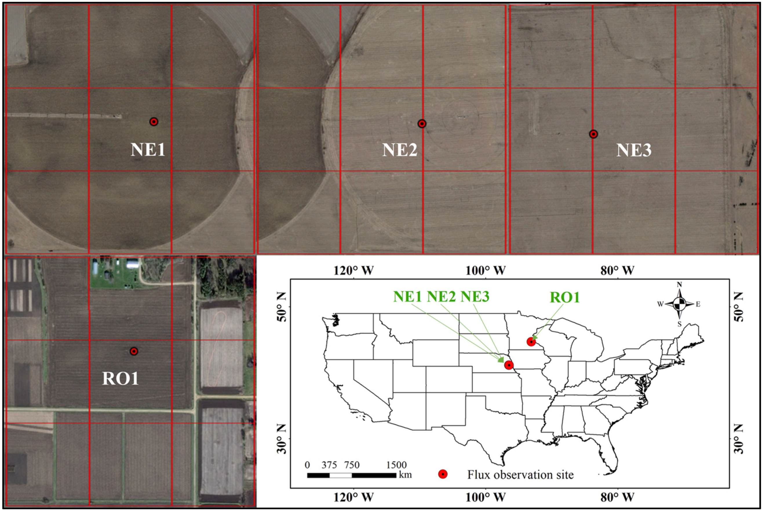
Figure 1. Locations of four flux sites (NE1, NE2, NE3, and RO1) and the MODIS pixel (red lines) with 250 m resolution corresponding to the sites.
Remotesensing 16 00341 g001
Figure 2. Time series of ground-measured daily maize GPP in NE1, NE2, NE3, and RO1 sites.
Remotesensing 16 00341 g002
Figure 3. SLN function based on the relationship between SLN and NMP with sufficient data from sites NE1, NE2, and NE3. The dots represent the original data. The hollow circle represents the averaged SLN at an interval of 0.03 NMP.
Remotesensing 16 00341 g003
Figure 4. (a) Mean square error of RF based on the out of bag error rate with different parameter combinations. (b) Importance of input variables in NE1, NE2, and NE3 sites for GPP based on RF.
Remotesensing 16 00341 g004
Figure 5. Distribution of evaluation metrics of test results for different combinations (A0: (a,e,i,m); A1: (b,f,j,n); A2: (c,g,k,o); and A3: (d,h,l,p)) using RF in NE1, NE2, and NE3 sites for 1000 running times. μ is the mean value and σ is standard error. The line is the fitted normal distribution curve. The column represents the data number.
Remotesensing 16 00341 g005
Figure 6. Scatter plots of A0 and A3 combinations, respectively, for NE1, NE2, and NE3 sites. (a,b): training in NE1 site and testing in NE2 site; (c,d): training in NE1 site and testing in NE3 site; and (e,f): training in NE3 site and testing in NE2 site. The red line is the fitting line between estimated GPP (GPPm) and ground-measured GPP (GPPg), and the dashed line is the 1:1 line.
Remotesensing 16 00341 g006
Figure 7. Validation of RF in RO1 site while trained in NE1, NE2, and NE3 sites. The red line is the fitting line between estimated GPP (GPPm) and ground-measured GPP (GPPg), and the dashed line is the 1:1 line.
Remotesensing 16 00341 g007
Figure 8. GPP estimation results of SVM, CNN, and ELM in RO1 site. The red line is the fitting line between estimated GPP (GPPm) and ground-measured GPP (GPPg), and the dashed line is the 1:1 line.
Remotesensing 16 00341 g008
Table 1. The details of the available daily data at four flux sites.
SiteLongitude (°W)Latitude (°N)Available YearData Size
NE1−96.476641.16512001, 2002, 2003, 2004, 2005, 2006, 2007, 2008, 2009, 2010, 2011, 20121945
NE2−96.470141.16492001, 2003, 2005, 2007, 2009~20121276
NE3−96.439741.17972001, 2003, 2005, 2007, 2009, 2011987
RO1−93.089844.71432009, 2011214
Table 2. Input variable combinations for comparison.
SymbolInput Variable Combination
A0NDVI + Tmean + Tmin + Tmax + SSR
A1NDVI + Tmean + Tmin + Tmax + SSR + SLN
A2NDVI + Tmean + Tmin + Tmax + SSR + NMP
A3NDVI + Tmean + Tmin + Tmax + SSR + SLN + NMP
Table 3. Comparison of the performance of RF, SVM, CNN, and ELM at NE1, NE2, and NE3 sites. The bolded font represents the variable combination that makes the highest accuracy for each ML method.
NSERMSEBiasCV
μσμσμσμσ
RFA00.95740.00211.86710.0432−0.01740.06210.18050.0046
A10.96530.00171.68480.0408−0.01150.05710.16270.0042
A20.96880.00151.59650.0371−0.00410.05350.15430.0040
A30.97030.00141.55960.03420.00290.05390.15080.0037
SVMA00.95890.00191.83570.0401−0.05210.06510.17720.0043
A10.96680.00161.64800.0378−0.01390.05560.15940.0038
A20.96990.00141.57030.03530.00640.05620.15170.0039
A30.97060.00141.55090.03630.01630.05690.14700.0038
CNNA00.95290.00591.96100.1151−0.15130.18480.18970.0112
A10.95530.00291.91030.0637−0.04540.18590.18470.0064
A20.96090.00291.78720.0647−0.02310.15350.17290.0066
A30.95970.00221.81520.0490−0.00310.17630.17550.0051
ELMA00.95780.00191.85950.0390−0.00040.06310.17950.0041
A10.96440.00161.70690.03740.00040.05670.16500.0038
A20.96810.00141.61460.03380.00140.85410.15600.0037
A30.96740.00151.63210.03630.00130.05420.15790.0039
Table 4. The comparison of RMSE and URMSE for ML methods introducing SLN and NMP or not introducing them in RO1 site. The unit is gC·m−2·day−1.
RMSEURMSE
RFA02.8372.771
A32.6542.213
SVMA02.5562.502
A32.6562.280
CNNA02.6292.627
A22.5392.417
ELMA02.5492.472
A22.5712.168
Disclaimer/Publisher’s Note: The statements, opinions and data contained in all publications are solely those of the individual author(s) and contributor(s) and not of MDPI and/or the editor(s). MDPI and/or the editor(s) disclaim responsibility for any injury to people or property resulting from any ideas, methods, instructions or products referred to in the content.