Spatial Estimation of Daily Growth Biomass in Paddy Rice Field Using Canopy Photosynthesis Model Based on Ground and UAV Observations

Abstract

Precision farming, a labor-saving and highly productive form of management, is gaining popularity as the number of farmers declines in comparison to the increasing global food demand. However, it requires more efficient crop phenology observation and growth monitoring. One measure is the leaf area index (LAI), which is essential for estimating biomass and yield, but its validation requires destructive field measurements. Thus, using ground and UAV observation data, this study developed a method for indirect LAI estimation based on relative light intensity under a rice canopy. Daily relative light intensity was observed under the canopy at several points in paddy fields, and a weekly plant survey was conducted to measure the plant length, above-ground biomass, and LAI. Furthermore, images from ground-based and UAV-based cameras were acquired to generate NDVI and the canopy height (CH), respectively. Using the canopy photosynthetic model derived from the Beer–Lambert law, the daily biomass was estimated by applying the weekly estimated LAI using CH and the observed light intensity data as input. The results demonstrate the possibility of quantitatively estimating the daily growth biomass of rice plants, including spatial variation. The near-real-time estimation method for rice biomass by integrating observation data at fields with numerical models can be applied to the management of major crops.

1. Introduction

To ensure stable food production in response to global population growth, it is necessary to increase unit yield in agriculture adapted to limited farmland resources and local environments such as climate and meteorology [1,2]. For this purpose, monitoring of crop growth and adapting appropriate cultivation management are required. Monitoring the growth of crops and properly managing their cultivation are skills that farmers have long developed empirically. However, despite rising global food consumption and production, the number of farmers is declining [3]. As a result, worldwide efforts are being made to overcome this problem through efficient and effective precision farming.

Efficient crop phenology observation and growth monitoring at the field level are critical in precision farming. This requires not only labor-saving operations but also extremely accurate yield estimation and prediction. In cultivation management, it is critical to understand the differences in growth stages due to differences in environmental factors (e.g., weather and field conditions in the year of planting) and different production management (e.g., varieties and fertilizer amounts). Monitoring the growth condition of the entire field is also a useful way to determine the effects of abnormal and extreme weather on crops, which are expected to become more frequent as a result of global warming. Precision farming, which replaces traditional farming methods (e.g., the use of fixed-point cameras and ICT), makes it possible to quantitatively grasp the growth status of fields at any time, either by visual identification or by automatic digital processing [4,5]. Furthermore, regular UAV observation allows for detailed field monitoring [6]. UAVs have enabled accurate identification of agricultural growth conditions at the individual level by taking photographs from low altitudes; however, the finer spatial scale requires equally detailed information on the time-series changes in growth. Despite the advancements in UAV technology, the realistic observation frequency is still once a week in consideration of flight planning, operation, data processing, and other aspects.

On the other hand, crop growth, especially biomass, is affected by temporal changes in sunlight, which is most closely related to the rate of photosynthesis. Precision farming, which requires detailed information on both spatial and temporal scales, has the potential to estimate and predict a field’s growth conditions spatiotemporally by combining fixed-point observations and UAV observations with meteorological data that can be input into crop growth models.

There are many cases related to the estimation of leaf area index (LAI) in applied research on remote sensing for precision farming [7,8,9,10,11,12]. This is because LAI is an essential parameter for input into crop models for biomass and yield estimation and prediction. Traditionally, obtaining LAI verification data has not been easy because it requires measurement by cutting samples; however, there is a method to indirectly estimate LAI based on the light environment (i.e., light transmission by leaves) under the canopy [13]. This method was derived by cutting the leaves of an herbaceous sample layer by layer and simultaneously measuring the light transmittance. In recent years, devices have evolved to measure LAI based on light transmission characteristics [14,15]. However, these measuring devices are not automated, thus requiring people to go to the site and take measurements. Furthermore, even with the use of an auto-measuring function, data can be measured at only one point on the device. Therefore, LAI can be estimated non-destructively, effectively, and spatially by estimating the light transmittance within a canopy using ground-based or UAV-based remote sensing observation data. Furthermore, the canopy photosynthesis model [13,16,17,18] used in several crop models allows photosynthetic photon flux density (PPFD) to correspond to diurnal changes in sun altitude. It allows for the geometric calculation of light absorption and transmission received by leaves, as well as the simulation of the amount of growing biomass per day by inputting diurnal changes in PPFD and time-series LAI [19,20,21]. Therefore, the integrated use of observed data in the field and numerical models can be expected to provide continuous growth monitoring both spatially and temporally.

The purpose of this study was to investigate observational methods for efficient indirect estimation of LAI, which is essential for biomass estimation and yield prediction, as well as to perform spatial estimation of daily biomass through the application of the canopy photosynthesis model. Data from ground- and UAV-based observations at two paddy rice field sites and rice cultivated in different years were used to assess a method for measuring the light environment under the rice canopy (relative light intensity at the top and bottom of the canopy). In addition, the time-series LAI estimated indirectly from the relative light intensity and the observed light intensity used in photosynthesis (PPFD) were applied to a canopy photosynthesis model for calculating the amount of growth biomass per day. The validity of this method was further examined by comparing the accumulative biomass with the above-ground biomass.

2. Materials and Methods

2.1. Model Description

2.1.1. Light Distribution under Canopy

The photosynthesis rate is determined by how much light is absorbed by the leaves under the canopy layer. The Beer–Lambert law can describe the light attenuation absorbed by leaves from the top to under the canopy using this equation [13]:

$$I_i=I_0\mathrm{e}\mathrm{x}\mathrm{p}(-K{F}_i)$$

(1)

whereas I_i is the horizontal light intensity at layer i in the canopy, I₀ is the horizontal light intensity, K is the extinction coefficient, and F_i is the leaf area index (LAI, m²/m²). I₀ denotes the photon flux density per unit leaf area per unit time on top of the canopy. The F_i reaches a maximum at the bottom layer of the canopy and shows the LAI under all layers. The relationship of the relative light intensity logarithm (I_i/I₀) in layers i and F_i is linear, with K as the slope. The extinction coefficient K is closer to 1 for horizontal leaves.

2.1.2. Canopy Photosynthesis Model

The canopy photosynthesis model based on Monsi and Saeki (1953) [13] has been widely used and modified by considering the light environment and the leaf morphology (e.g., [16,17,18,22]). It is based on a mathematical model that analyzes the light response to changes in the sun’s elevation during the day and the absorption and transmission processes of light received by leaves for each variety of plant. Daily productivity (biomass) can be estimated in time series by inputting the incident light intensity and LAI (e.g., [20,21]).

In this study, the canopy photosynthesis model modified by Anten (1997) [18,19] was used, in which the total incident light on the top of the canopy is divided into direct and diffuse lights. This model is based on the calculation of the photosynthetic rate in each layer by separating the sunlit and the shaded leaves.

Light intensity received by sunlit leaves and shaded leaves [18]: The canopy is divided vertically into multiple layers, and the intensity of light received by the leaves in each layer is calculated. The sunlit leaves receive both direct and diffuse light, whereas shaded leaves receive only diffuse light. The absorbed light intensity of the sunlit leaves (I_sl,i, μmol/m²/s) in layer i is expressed by:

$$I_{sl,i}=I_{sh,i}+\frac{O{I}_{0b}}{\sin {\beta }_s}$$

(2)

where I_sh,i (μmol/m²/s) is the absorbed light intensity received by shaded leaves in layer i, O is the projected area of leaves from the view of the sun, I_0b is the direct light (μmol/m²/s) received at the horizontal plane above the canopy, and β_s is the sun elevation angle. O is a parameter that varies depending on the leaf slope and the sun elevation and is calculated by dividing the slopes into three classes [17]:

$$O=f_{15}{O}_{15}+f_{45}{O}_{45}+f_{75}{O}_{75}$$

(3)

where O₁₅, O₄₅, and O₇₅ are the projected area of slope of the leaves from 0 to 30, 30 to 60, and 60 to 90 degrees, respectively, and f₁₅, f₄₅, and f₇₅ are the fraction of the three slope classes. In this study, f₁₅, f₄₅, and f₇₅ were set based on the growing conditions of rice leaves of 0.6:0.3:0.1, respectively.

The projected area of the leaves, O₁₅, O₄₅, and O₇₅ of the three classes, can be calculated using Equation (4) when the sun elevation angle β_s is higher than the leaf slope, whereas Equation (5) is used when it is lower than the leaf slope. O₄₅ and O₇₅ are calculated similarly.

$$O_{15}=\sin {\beta }_s\cos \left(15\right)$$

(4)

$$O_{15}=\frac{\pi }{2}[\sin {\beta }_s\cos \left(15\right){\sin }^{-1}\left(\frac{\tan {\beta }_s}{\tan \left(15\right)}\right)+({\sin }^2{\beta }_s+{\mathrm{s}\mathrm{i}\mathrm{n}}^2\left(15\right){)}^{0.5}]$$

(5)

Furthermore, in Equation (1), I_sh,i is expressed by:

$$I_{sh,i}=\frac{K_d}{{\left(1-\sigma \right)}^{0.5}} (I_{d,i}+I_{bd,i})$$

(6)

where K_d is the extinction coefficient for diffuse light, and σ is the leaf scattering coefficient and was set as 0.3 after considering that the reflectance and transmittance of rice leaves is relatively high. I_d,i is the light intensity of the diffuse light received by the horizontal plane in layer i:

$$I_{d,i}=I_{0d}\mathrm{e}\mathrm{x}\mathrm{p}(-K_d{F}_i)$$

(7)

where I_0d (μmol/m²/s) is the light intensity of the diffuse light received by the horizontal plane above the canopy. I_bd,i, which is the diffuse light derived from the direct light at layer i, is calculated by:

$$I_{bd,i}=I_{d,i}-I_{bb,i}$$

(8)

I_bb,i indicates the light intensity of non-diffusive direct light in layer i. I_b,i and I_bb,i are indicated by Equations (9) and (10), respectively:

$$I_{b,i}=I_{0b}\mathrm{e}\mathrm{x}\mathrm{p}(-K_b{{\left(1-\sigma \right)}^{0.5}F}_i)$$

(9)

$$I_{bb,i}=I_{0b}\mathrm{e}\mathrm{x}\mathrm{p}(-K_b{F}_i)$$

(10)

where K_b is the extinction coefficient of direct light and is expressed by:

$$K_b=\mathrm{O}/\sin {\beta }_s$$

(11)

where the sun elevation angle β_s can be calculated using the latitude and longitude of the study site.

In this model, the attenuation of diffuse light within the canopy is assumed to decrease, which follows the Beer–Lambert law (Equation (1)) [13].

Photosynthetic rate in each layer [18]: The photosynthetic rate per unit area in layer i (P_N,I, μmol CO₂/m²/s) is expressed by:

$$P_{N,i}=f_{sl,i}{P}_{sl,i}+{(1-f}_{sl,i}) P_{sh,i}$$

(12)

The fraction of sun leaves f_sl,i is expressed as follows:

$$f_{sl,i}=\exp \left(-K_b{F}_i\right)$$

(13)

where P_sl,i and P_sh,i show the photosynthetic rate (μmol CO₂/m²/s) of sunlit leaves and shaded leaves in layer I, respectively. They are calculated using the light response curve of photosynthesis approximated by a non-rectangular hyperbola [23].

$$P_{sl,i}=\frac{\phi I_{sl,i}+P_m-\sqrt{{\left(\phi I_{sl,i}+P_m\right)}^2-4\phi I{P}_m\theta }}{2\theta }-r_D$$

(14)

where ϕ is the initial slope of the light response curve of photosynthesis, P_m is the photosynthetic rate per unit area under saturated light, θ is the curvature, and r_D is dark respiration. P_sh,i is also calculated by inputting the light intensity received by shaded leaves by replacing I_sl,i with I_sh,i (Equation (6)). Using Equation (12), P_N,i can be calculated from all derived values $(f_{sl,i},P_{sl,i},P_{sh,i})$. By accumulating P_N in all layers i, the carbon dioxide fixed by photosynthesis for a given LAI can be estimated.

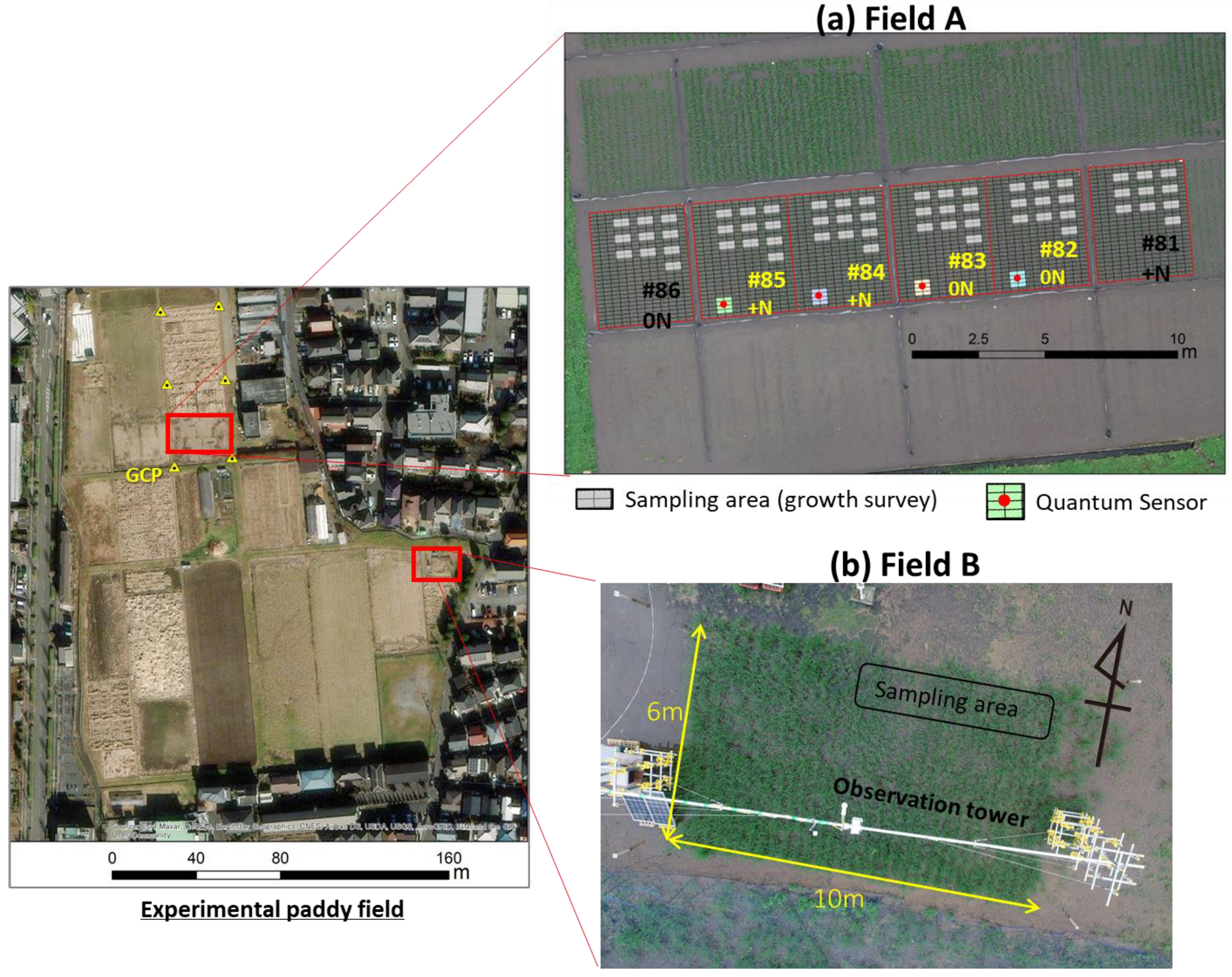
2.2. Experimental Site

Two fields with alluvial cray loamy soil were used in the experimental paddy field of Tokyo University of Agriculture and Technology (N35.666, E139.471, 49 m above sea level) (Figure 1). The area’s climatic conditions are mild and generally warm, with a mean annual temperature and precipitation of 15 °C and 1530 mm, respectively.

The experiment used Koshihikari (Japonica), a rice model cultivar that is mostly cultivated in various parts of Japan. The experiments were established in three cropping seasons: fields A and B on 3 June 2020 and in Field B on 20 May 2021 and 30 May 2022. Three seedlings per hill were transplanted every 30 cm (between rows) by 15 cm (between plants) in fields A and B. Field A was divided into non-fertilized (0N) and fertilized (+N) areas for three replicates (total 6 plots) with plot sizes of 4.2 m by 3.6 m. Meanwhile, Field B had a plot size of 7.8 m by 6.0 m and was not fertilized (0N) (Figure 1a).

Field A was used for UAV-based observation in 2020. Field B was used for ground-based observation using the tower with a 3 m height (Figure 1b) and by hand from 2020 to 2022. With this setup, we can make comparisons between fields under the same meteorological conditions within a year (fields A and B in 2020) and determine yearly differences from 3 year observations (Field B in 2020 to 2022).

2.3. Estimation Procedures of Daily Growth Biomass

Figure 2 shows the procedures to estimate daily growth biomass based on the canopy photosynthesis model (Section 2.1) using daily or weekly LAI estimated by ground- and UAV-based remote sensing (Section 2.4 and Section 2.5) and incident light intensity with 10 min intervals (Section 2.6).

As for the other input parameters, sun elevation angle β_s was calculated in 10 min intervals using the day of the year and the hour:minute in Japan standard time and the latitude and longitude at the experimental field (N35.666, E139.471). Furthermore, the extinction coefficient K_d was determined by using the daily relative light intensity (I/I₀) (Section 2.4.1) and actual measured LAI at Field A (Section 2.4.5). As for the parameters of the light response curve of photosynthesis, P_m: 21, ϕ: 0.08, θ: 0.8, and r_D: 0.5 were set per references [24,25], which described the results by measuring the photosynthetic rate for Koshihikari.

As an output, the photosynthetic rate (μmol CO₂/m²/s) at every 10 min interval was accumulated for one day (mol CO₂/m²/d) and then converted to daily biomass (CH₂O g/m²/d) and obtained accumulated biomass (CH₂O g/m²). The photosynthesis rate, daily growth biomass, and accumulated biomass were compared with the incident light intensity and the measured above-ground biomass (AGB, g/m²), and these relationships were discussed.

2.4. Observation Data

The observation data gathered in fields A and B are described as follows (

Table 1. Summary of observation data in fields A and B.

	Field A	Field B
Observation year	2020	2020, 2021, 2022 *
Relative light intensity under the canopy (daily)	4 plots	5 points
Incident PPFD (10-min)	Downward and upward PPFD (μmol/m2/s)
Ground-based remote sensing (daily/weekly)	-	VC, GR, NDVI
UAV-based remote sensing (weekly)	CH (m), GR, NDVI	-
Growth survey (weekly)	PL (m), AGB (g/m2), LAI (m2/m2)	PL(m), AGB (g/m2)

* No observation of daily VC or GR in 2022.

).

2.4.1. Relative Light Intensity under Rice Canopy

The quantum sensors, which are sensitive to visible light, with memory (DEFI2-L, JFE Advantech, Hyogo, Japan) were set at five points in Field B (Figure 1b) and at four points in plots of Field A (Figure 1a) to measure the transmitted light at the bottom of the canopy (I_t) and the incident light at the top of the canopy (I_0t) at time t. Each sensor was placed 15 cm between each plant.

For sensor calibration, measurements were performed using all sensors under the same sunlight conditions for about two weeks before and after the field measurement. The measurement interval was every 1 min. The data measured from 7:00 to 18:00 were used to determine the daily relative light intensity (I/I₀). In general, the relative light intensity measured under cloudy weather is used to determine the leaf extinction coefficient [16]. However, in cloudy conditions, the observed data are limited, making it difficult to select usable data.

In this study, we calculated the relative light intensity representing daily values using the 660 values measured at 1 min intervals under various sky conditions during the daytime using the following equation [26,27]:

$$\frac{I}{I_0}=\frac{1}{n}\sum _{n=1}^{660}\frac{I_t}{I_{0t}}$$

(15)

2.4.2. Incident Photosynthetic Photon Flux Density (PPFD)

Two photosynthetic photon quantum sensors (LI-190SB, Licor Inc., Lincoln, NE, USA) were installed at the top of tower in Field B (Figure 1b) to measure both downward and upward PPFD (μmol/m²/s). The LI-190SB can scan every second, and the data were saved as the 10 min mean at 10 min intervals. These PPFDs were used as the input parameters of the incident light intensity every 10 min after dividing the direct and diffuse components (as described in Section 2.6).

2.4.3. Ground-Based Remote Sensing

A single-lens reflex camera (D5300; Nikon, Tokyo, Japan) with a wide-angle lens (EX/DC; SIGMA, Kanagawa, Japan) in a waterproof case was installed at the nadir direction in a tower with a height of 3 m in the Field B setup (Figure 1b). The RGB image was captured with a fixed aperture of f:5.6, auto shutter speed, and auto white balance. Images were saved in JPEG format every 10 min during the daytime in the periods from 9 July to 9 September 2020 and from 28 May to 6 September 2021. A total of 36 images per day captured from 9:00 to 15:00 were used to calculate the green ratio (GR) and vegetation coverage (VC) in the region of interest (ROI) of about 1.6 m by 1.6 m for each image (Figure 1c). The GR was computed using the following equation:

$$GR=\frac{G}{R+G+B}$$

(16)

where R, G, and B represent the red, green, and blue bands, respectively. VC was calculated as the ratio of the area of green leaves. As for the detection of green leaves, we separated all pixels into the green area and the other area using the International Commission on Illumination (Commission Internationale de l’Eclairage: CIE) L*a*b*, which were computed from tristimulus values X, Y, and Z, respectively. The green area was segmented using the threshold of the a* value for each image. The calculated values of GR and VC from 36 images were averaged as daily representative values in Field B.

In addition, three bands of near infrared (NIR), red, and green were captured by hand using a multi-spectral camera (HAWC; TETRACAM Inc., Chatsworth, CA, USA) at five points at a height of about 1 m at around 9:00 once a week in a rice growth survey. This multi-spectral camera had the incident light sensor. The image taken under the different sunlight conditions was calibrated as a reflectance factor using the optional software PexelWrench2 (TETRACAM Inc.), and then the Normalized Difference Vegetation Index (NDVI) was calculated using the following equation:

$$NDVI=\frac{NIR-R}{NIR+R}$$

(17)

We used the average measurements of the NDVI at the five points as the weekly representative of the relative light-intensity measurement for Field B.

2.4.4. UAV-Based Remote Sensing

To obtain the spatial and temporal information related to rice growth, the canopy surface model (CSM) and the ortho-mosaic image with spectral bands were generated using the overlapping images taken by a UAV. Ground control points (GCPs) were set in Field A using the total station and auto level by conducting traverse surveying and leveling. The Japan Geodetic Datum 2011/Plane Rectangular Coordinate System Zone 9 was referred to for the coordinates of the GCPs as a map projection. These were fixed at the six points around the edge of the paddy field (Figure 1). A set of overlapping images covering the whole field was taken using a UAV (Inspire 2; DJI, Shenzhen, China) equipped with an RGB camera (Zenmuse X4S; DJI) and a multispectral camera (RedEdge-MX; MicaSense, Seattle, WA, USA) with five bands of B, G, R, red edge, and NIR. The flight altitude was fixed at 30 m above the rice canopy with a forward and lateral overlap rate of 85%.

The flight of the UAV was conducted between 9:00 and 10:30, when the sun elevation angle was relatively high (around 50–70 degrees) and the sky was clear. Since the multispectral camera was equipped with an incident spectral-light sensor, the correction of reflectance factors could be performed during post-processing by taking a grayscale board for correction before the flight. Two kinds of aerial images with RGB and multi-spectral bands were taken every week from the beginning of June to the end of August in 2020 (10–13 flights used).

Generation of canopy surface model: The Metashape Professional (ver. 1.5.1, Agisoft), a Structure from Motion (SfM) software, was used to generate a time-series digital surface model (DSM) by processing the UAV-acquired RGB images on days with 10 flights. First, tie points were automatically identified from the overlapping aerial images; then, the tie points were used to calibrate camera parameters such as the focal length of the lens, principal point positioning, and radial and tangential distortions. The parameters of external orientation (camera position and tilting angle) were estimated using the detected tie points and four installed GCPs; then, a 3D model was generated. This processing was carried out to achieve a GCP accuracy to within 1 pixel. A DSM with a spatial resolution of approximately 9 mm/pixel was developed. Using the DSM, the CSM was calculated from the distance between the DSM of each observation day (DSM_n) and the first DSM after transplanting (DSM1st, defined as the reference plane). The value of the CSM was defined as the canopy height (CH). This relation is mathematically expressed as

$${CSM}_n={DSM}_n-{DSM}_{1st},$$

(18)

where n represents the observation dates [28].

Generation of ortho-mosaic images: Time-series ortho-mosaic images with multispectral bands were generated from each set of multispectral images taken during a total 10 flights at Field A using the same SfM software, Metashape. Each ortho-mosaic image was generated after creating the DSM to within 1 pixel (14 mm) error using the same GCPs.

Calculation of CH, NDVI, and GR: After generating the CSMs and ortho-mosaic images, we created polygons with a minimum size of a 30 cm × 15 cm rectangle, which corresponded to one hill of rice plants. Then, the mean values of the CH, NDVI, and GR were calculated in each polygon.

2.4.5. Rice Growth Survey

In Field A, plant length (PL, m), LAI, and AGB (g/m²) were measured weekly for four hills in each plot, as shown in the gray area of Figure 1b. LAI was measured using an automatic area measurer (AAM-9; Hayashi Denko, Tokyo, Japan). On the other hand, AGB was obtained by measuring the dry weight of plant organs that were oven-dried for 72 h at 80 °C. In Field B, PL was measured at five points for two hills, whereas AGB was measured weekly from the two hills outside the ROI. The number of tillers for the target hills was also counted. The measuring and sampling areas in fields A and B are shown in Figure 1a,b, respectively.

The actual measured LAI was used to determine the extinction coefficient K_d by using relative light intensity (I/I₀), whereas the AGB was used to compare the daily growth production and accumulated biomass estimated with the canopy photosynthesis model (Section 2.1.2).

2.5. LAI Estimations

LAI can be calculated using the relative light intensity (I/I₀) and K_d in Equation (19).

$$LAI=-\frac{1}{K_d}\mathrm{l}\mathrm{n}(\frac{I}{I_0})$$

(19)

In this study, the estimation formulas of relative light intensity (I/I₀) were derived by comparing the variables of daily VC, daily and weekly GR, weekly NDVI, and weekly CH from ground- and UAV-based remote sensing.

2.6. Direct and Diffuse Light Intensity Divided from Incident Global PPFD

According to the canopy photosynthetic model used in this study, the input light intensity needs to divide the direct and diffuse components (Equations (2) and (7), respectively). In previous studies, it was proposed to estimate the diffuse ratio (DR) proposed by using the clearness index (CI). The CI is the ratio of the solar radiation at the top of the atmosphere to the global solar radiation measured at the ground level [29]. The direct and diffuse radiations have not been observed as public meteorological data; therefore, it was necessary to estimate them using global solar radiation (e.g., [30,31,32]), which is commonly observed worldwide [33].

First, the formula was derived to estimate the diffuse ratio from the CI by using the global and diffuse solar radiations observed at the campus of Tokyo University of Agriculture and Technology, which is approximately 2 km away from the experimental site.

$$\begin{gathered} DR=1 (CI \le 0.250) \\ DR=7.511{CI}^3-10.894{CI}^3+3.112CI+0.782 \left(0.250<CI\le 0.775\right) \\ DR=0.145 (0.775<CI) \end{gathered}$$

(20)

Then, we integrated the amount of extraterrestrial spectral irradiance (W/m²/μm) in the visible wavelength (0.4–0.7 μm) [34] by converting it to the unit of photon flux density (μmol/m²/s) and obtained the extraterrestrial PPFD as a constant of 2405 μmol/m²/s (PPFD₀) [35]. The clearness index of PPFD (CI_ppfd) was calculated using the downward PPFD (PPFD_g) measured at Field B via:

$${CI}_{ppfd}=\frac{{PPFD}_g}{{PPFD}_{toa}}$$

(21)

$${PPFD}_{toa}={\mathrm{P}\mathrm{P}\mathrm{F}\mathrm{D}}_0{\left(\frac{{\mathrm{r}}_0}{r}\right)}^2\sin {\beta }_s,$$

(22)

where (r₀/r)² is the correction of the inverse square between r₀ (the mean earth–sun distance) and r (the earth–sun distance) on the observation day. Here, CI_ppfd was substituted for CI in Equation (20) to obtain DR.

After calculating DR, the downward PPFD was divided into diffuse PPFD and direct PPFD. In addition, the upward PPFD was multiplied by the ratio of diffuse and direct components. Each value subtracted from diffuse PPFD and direct PPFD was used as the diffuse and direct light-intensity incident on the canopy (I_0d and I_0b) in 10 min intervals.

3. Results and Discussion

3.1. Rice Growth Survey

The results of the weekly rice growth survey for PL, AGB, and LAI in Field A in 2020 and for PL and AGB in Field B for 3 years are shown in Figure 3. There were four kinds of sampling areas: two non-fertilized plots (0N, #82, and #83) and two fertilized plots (+N, #84, and #85) in Field A (Figure 1b). The results show growth differences between 0N and +N starting from 35–40 days after transplanting (DAT) (Figure 3a). In Figure 3c, LAI declined after its peak around DAT60 in all plots (fertilized and non-fertilized plots). This shows the same trends as the study conducted in 2018 and 2019 by Peprah et al. [28]. In Field B, a total of 10 plants were sampled in the area where the 5 photon sensors were placed. The mean PL and AGB of the sample plants showed an increasing trend from 2020 to 2022 (Figure 3d–f).

3.2. Weekly Change in Canopy Height Calculated from Canopy Surface Models

Figure 4a shows the results of CH calculated from aerial drone images taken in Field A. Differences in CH began to appear between the non-fertilized and fertilized plots from around 40 DAT, which coincides with the actual PL measurement (Figure 3a). Although it was not obvious from the seasonal changes in PL (Figure 4a), CH began to decrease slightly from around 75 DAT (heading stage). This can be explained by the method used to obtain the PL and CH measurements. PL is measured from the soil surface to the highest tip of the rice plant stretched by hand when measuring with ruler, whereas CH is the height in its natural state, without stretching the plant. Because the grain begins to fill and mature, the rice plants tend to bend toward harvesting.

The relationship between the measured PL and CH (Figure 4b) is expressed in a linear equation (CH = 0.993 × PL −0.286) with a slope nearly equal to 1.0. This indicates that a highly accurate canopy surface model (CSM) was obtained using aerial images taken by a UAV.

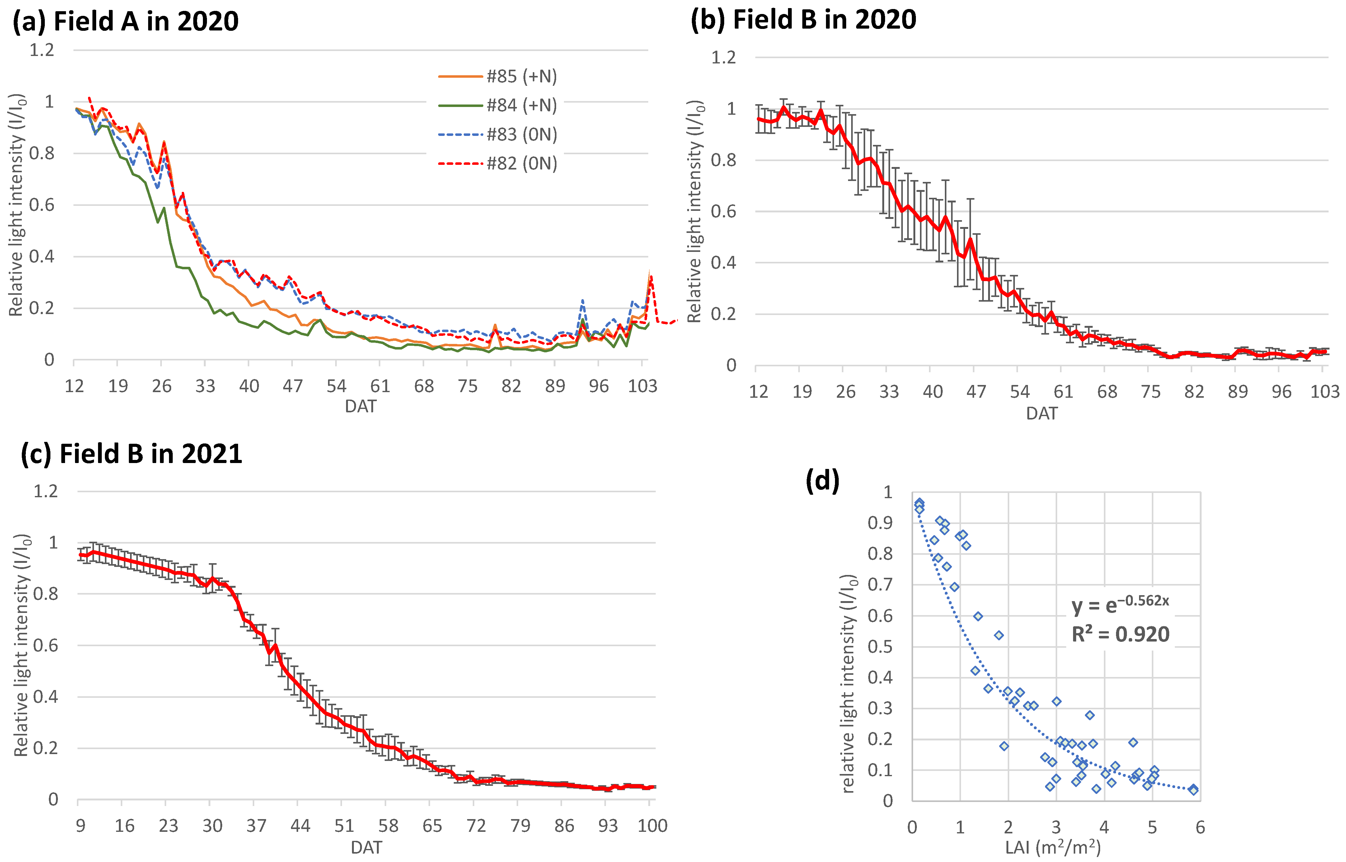
3.3. Daily Change in Relative Light Intensity (I/I₀) and the Extinction Coefficient (K_d)

The relative light intensity (I/I₀) is the light transmittance of leaves under the canopy and a parameter used to estimate the LAI (Equation (1)) via a non-destructive method. The daily average of relative light intensity (Equation (15)) in Field A in 2020 and in Field B in 2020 and 2021 is shown in Figure 5. There were clear differences between non-fertilized and fertilized plots, as shown in Figure 5a. The patterns of non-fertilized plots (#82 and #83) in Field B showed different trends. Even on the same transplanting date (3 June), differences in relative light intensity were seen in different fields due to differences in growth during the tillering stage. In particular, the transmittance decreased from 3 weeks to 9 weeks after transplanting depending on whether the field was fertilized or not fertilized.

During the beginning of I/I₀ observation in 2021, DAT from 12 (30 May) to 22 (10 June) was linearly interpolated because the sensor was submerged in water and the data could not be used (Figure 5c). The error bar shows the standard deviation of five points of the quantum sensors measurement in Field B (Figure 5b,c). Comparing Field B in 2020 and 2021, variations in the five measurement points were seen, especially in 2020. From around 70–75 DAT (heading stage), I/I₀ was stable, with a relative light intensity of less than 0.1 (Figure 5b,c).

The extinction coefficient (K_d) was derived from the relationship between relative light intensity and the measured LAI using data observed from early to late growth (Figure 5d). In this study, the K_d value was 0.562, which was found to be very close to the value in existing studies for the extinction coefficient of rice (e.g., [36,37]). Strictly speaking, it is known that the extinction coefficient differs depending on the growth stage [36]. However, in the canopy photosynthesis model used in this study, described in Section 2.1.2, the extinction coefficient of the leaves was assumed to be constant.

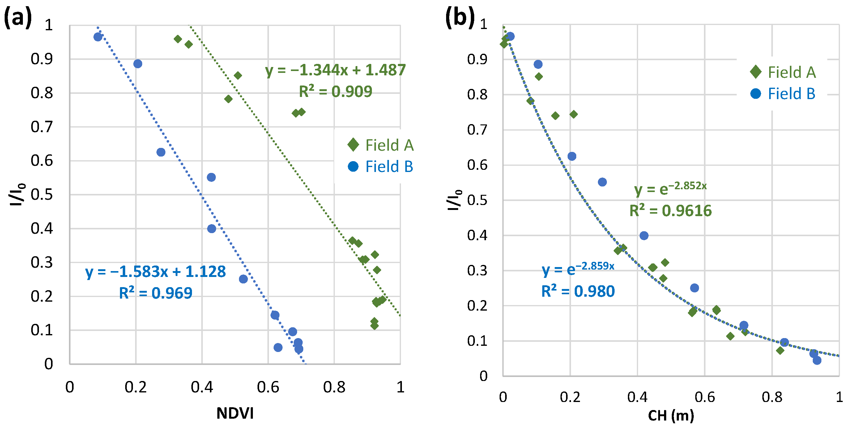
3.4. Relations of Relative Light Intensity with the Parameters of Ground- and UAV-Based Observations

The relationship between measured relative light intensity (I/I₀) and daily or weekly observation data (VC, GR, NDVI, and CH) obtained using ground- and UAV-based remote sensing methods was determined to obtain the optimal parameters for estimating the LAI (Figure 2).

3.4.1. Daily VC and GR at Field B in 2020 and 2021

Figure 6 shows the negative relationships between daily VC, GR, and I/I₀ at Field B in 2020 and 2021. At the early stage of growth (I/I₀: 0.95 to 0.8), the VC and GR increased quickly in 2020. Moreover, when the I/I₀ became 0.8 or less, VC (in 2020 and 2021) and GR (in 2020 only) increased with an almost constant slope. Comparing the two years, there were no major differences in the distribution for VC; however, the distributions of GR were significantly different between 2020 and 2021. It seems that other factors may have been influencing GR [38,39,40]. Even when the white balance was set, differences depending on the camera maker were observed. It is inefficient to set up a grayscale or color chart in the field and process lots of images. When using VC as an estimation parameter, the image resolution must be high to calculate the percentage of pixels identified as leaves. Therefore, it is considered difficult to calculate VC using UAV images compared to ground-based images. The use of an RGB camera in ground-based remote sensing is suitable for observing phenology. However, there are still issues to be solved when using it as an image index for estimating physical quantities.

3.4.2. Weekly NDVI and CH at Field B in 2020 to 2022

Figure 7 shows the relationship of I/I₀ with the NDVI and CH obtained every week for three years from 2020 to 2022 during growth surveys in Field B. The CH was calculated from the measured PL in the growth survey using an estimation formula (CH = 0.993 × PL − 0.286).

The NDVI is a linear equation, whereas CH is an exponential function, and a well-fitting regression equation was derived. Comparing years, although there was a slight difference in the intercept for the NDVI, the slope was almost the same. This is because the multispectral camera (HARK) used was equipped with an incident light sensor. As a result, internal processing could correct the differences in solar radiation condition on the day and time the photo was taken. This result is significantly different from the GR result (Figure 6b) obtained using the uncalibrated camera images [38,41].

Regarding CH, I/I₀ = 1 at the top of the canopy can theoretically be regarded as the intercept, as defined by the Beer–Lambert law. There was almost no difference in the coefficient related to CH (2.86, 2.88 and 3.02), corresponding to the optical thickness within the rice canopy, over the three years of rice cultivation using the same variety and transplanting density. Since the physical quantity of height was used as a variable, there is a high possibility that plant height can be used in conventional growth surveys.

3.4.3. Weekly NDVI and CH from UAV-Based Observation at Field A in 2020

The relationship between the NDVI, GR, CH, and relative light intensity based on UAV observation in Field A is shown in Figure 8. Slight differences in the coefficients were seen in plots with or without fertilizer application. The difference in the amount of growth due to different fertilization is also shown in Figure 3. CH is an exponential function, and NDVI and GR show the linear regressions (Figure 7). The coefficients of the three types of regressions were lower in non-fertilized (0N) plots, indicating that even with the same NDVI, GR, and CH values, non-fertilization had high relative light intensity. For instance, the transmittance was different in the same leaf area and with different leaf characteristics (e.g., thickness). Although it also depends on the variety, the coefficient may have been smaller in non-fertilized plots because the rice plants grew taller but with fewer leaves. Regarding such differences in the coefficients of regression equations, further investigation is required based on differences in varieties and fertilizer amounts.

3.4.4. Comparison with Field A and Field B in 2020

Non-fertilized plots in Field A and B were compared in 2020 observations (Figure 9). In terms of the NDVI, there was a slight difference in the slope and a large difference in the intercept, which was largely due to the differences in the cameras used and the spatial resolution (distance to the rice plants). In contrast, there was no difference in CH between fields A and B—the coefficients were the same even in different fields when the fertilization conditions were the same.

The generation of DSM using overlapping images taken with a UAV was relatively unaffected by the weather or the time of day; therefore, the possibility of using time-series CSM to obtain spatially continuous information about the entire field is high. Furthermore, it is an effective method to observe the canopy height (corresponding to rice growth) from RGB images acquired with a UAV without using a calibrated multispectral camera [28]. However, satellite images (e.g., vegetation indexes, etc.) can be used to expand to a wider regional scale [6,42,43], but further knowledge of the relationship between canopy height and satellite data is required [44,45].

3.5. Daily Biomass Estimation at the Field Scale

The daily LAI was estimated using the observation results of daily relative light intensity (I/I₀) with a K_d of 0.562 (Equation (19)). Then, the daily biomass (CH₂O g/m²/d) at Field B in 2020 and 2021 was assessed using the incident diffuse and direct light intensity (I_0d and I_0b, μmol/m²/s) in 10 min intervals divided from the observation data of upward and downward PPFD (Equations (1)–(14)). Figure 10 shows the sampled AGB, estimated daily biomass and accumulated biomass (Figure 10a,b, respectively), and the daily amounts of direct and diffuse PPFD (mol/m²/d) during the growing period (Figure 10c,d, respectively). Based on the results, the daily biomass amount varied depending on the light intensity. In addition, as LAI increased with growth, the daily biomass also increased before peaking at the early stage of heading (DAT60–70) in 2020 and 2021. After heading, the light intensity fluctuated depending on the daily weather. Due to unfavorable weather for one week around DAT85–90 in 2021, the influence of daytime light intensity was found to decrease in daily biomass and accumulated biomass. Furthermore, the time-series changes in accumulated biomass and AGB measured by weekly growth surveys showed closer values in 2020 and 2021. The root mean square error (RMSE) and relative RMSE (%) of the measured AGB and biomass accumulated using the estimated LAI from the measured I/I₀ in 2020 and 2021 were 112.2 g/m² (22.7%) and 109.9 g/m² (15.8%), respectively. This result is in good agreement to measure the AGB and showed good accuracy when compared with our previous study [28].

To estimate daily biomass in all of Field A, the LAI with mesh data 15 cm by 30 cm were estimated weekly with Equation (23) using the CSM generated with the UAV images.

$${LAI}_{ch}=-\frac{1}{K_d}\mathrm{l}\mathrm{n}(e^{-\tau \times CH})$$

(23)

where LAI_ch is the LAI estimated from CH, and τ is the optical thickness within the rice canopy. τ was determined to be 2.95 based on the relationships between I/I₀ and CH (Figure 7b, Figure 8c and Figure 9b). Figure 11 shows the relationship between the measured LAI and the estimated LAI_ch at four points of quantum sensors (Figure 1a). The slope of the linear regression equation was approximately 1.00, and the intercept was close to the mean error. There was a tendency to underestimate the value slightly due to a systematic error. Tan et al. [46], in a study similar to this one, proposed an estimation method using the NDVI based on the Beer–Lambert law for non-destructive LAI estimation. However, estimation using the NDVI as a variable depends on the multispectral camera used. In this study, we confirmed that the relationship between the physical quantity of canopy height and relative light intensity showed an insignificant difference in the coefficients of the model equation in different fields and in different years. The results show that the LAI can be estimated using a non-destructive method with spatial data observed with a UAV in studies similar to existing ones (e.g., [28,46,47]). It shows that this method is versatile.

The weekly estimated LAI_ch for all meshes was interpolated to the daily LAI_ch by spline; then, the accumulated biomasses day by day from 14 (17 June) to 97 (8 September) DAT were estimated spatially in Field A (Figure 12).

Daily spatial changes in the biomass and the differences between non-fertilized and fertilized plots can be observed. As shown in the estimation results of time-series accumulated biomass at the quantum sensor points in plots #84 and #83 (Figure 13a,b), daily growth and its accumulated amount fit well with the AGB measured at the sampling area. The RMSE and relative RMSE were also similar to the results of accumulated biomass using the measured I/I₀ (Figure 10a,b).

The AGB estimation result showed an almost one-to-one relationship in plot 84 (Figure 13c), whereas there was a larger difference in plot 83 (Figure 13d). This is demonstrated by the larger RMSE in plot 83 than plot 84, of 39.3 and 90.7, respectively. After the heading stage, the lower leaves gradually wither; therefore, it is necessary to consider the estimation method after heading in the future.

With the spread of UAVs, applied research on precision farming using UAV images is increasing. Although there are many research examples using machine learning, there is a possibility that it cannot be applied to observed data due to different observation conditions (ex. differences in field or year) depending on the camera used. Therefore, engineers and researchers are required to understand the essence of observational data obtained through remote sensing and then use their judgment to determine which images can be used as training data.

In this study, a method to estimate the relative light intensity under a rice canopy using a simple regression model based on limited observation data is proposed. From these results, it is possible to understand the amount of daily growth by using LAI time-series data estimated from the relative light intensity under the rice canopy based on the remotely sensed observation and the direct and diffuse PPFD data used for photosynthesis.

In recent years, the use of spatiotemporal data from ground observation, UAVs, and satellite remote sensing is expected to be utilized in smart agriculture, as it has been used in an integrated manner with numerical models based on observational data [6,48]. However, since PPFD is not a frequent meteorological observation item, research on calculating direct and diffuse PPFD utilizing global solar radiation, ground observation, and meteorological satellite data is required.

4. Conclusions

This study examined an efficient and nondestructive method for estimating the LAI for precision farming via remote sensing techniques. The method was applied to a canopy photosynthesis model that calculates the photosynthetic rate considering temporal changes in sun incident light. The spatial estimation of daily biomass and accumulated biomass in a paddy field was also conducted.

The results show that daily rice plant growth can be quantitatively estimated, including spatial variation, by utilizing estimated LAI. It was estimated using weekly ground-based or UAV-based data and a canopy photosynthesis model with a high temporal resolution and PPFD with 10 min observations as input data. Conventional simulations based on numerical models have been limited to one-dimensional predictions representative of a farm field because spatio-temporal observation data were unavailable. With the recent global promotion of precision farming and the widespread use of UAVs, the possibility of near-real-time estimation and prediction has been demonstrated through the integrated use of observation data based on remote sensing. It is concluded that the near-real-time estimation of rice biomass by data assimilation with numerical models based on field observation data is an effective method for the cultivation management of major crops.

References

1. Molotoks, A.; Smith, P.; Dawson, T.P. Impacts of Land Use, Population, and Climate Change on Global Food Security. Food Energy Secur. 2021, 10, e261. [Google Scholar] [CrossRef]
2. FAO; IFAD; UNICEF; WFP; WHO. Urbanization, agrifood systems transformation and healthy diets across the rural–urban continuum. In The State of Food Security and Nutrition in the World 2023; FAO: Rome, Italy, 2023. [Google Scholar] [CrossRef]
3. FAO. World Food and Agriculture—Statistical Yearbook 2020; FAO: Rome, Italy, 2020. [Google Scholar] [CrossRef]
4. Dworak, V.; Selbeck, J.; Dammer, K.H.; Hoffmann, M.; Zarezadeh, A.A.; Bobda, C. Strategy for the Development of a Smart NDVI Camera System for Outdoor Plant Detection and Agricultural Embedded Systems. Sensors 2013, 13, 1523–1538. [Google Scholar] [CrossRef] [PubMed]
5. Lee, K.J.; Lee, B.W. Estimation of Rice Growth and Nitrogen Nutrition Status Using Color Digital Camera Image Analysis. Eur. J. Agron. 2013, 48, 57–65. [Google Scholar] [CrossRef]
6. Maes, W.H.; Steppe, K. Perspectives for Remote Sensing with Unmanned Aerial Vehicles in Precision Agriculture. Trends Plant Sci. 2019, 24, 152–164. [Google Scholar] [CrossRef] [PubMed]
7. Duan, S.B.; Li, Z.L.; Wu, H.; Tang, B.H.; Ma, L.; Zhao, E.; Li, C. Inversion of the PROSAIL Model to Estimate Leaf Area Index of Maize, Potato, and Sunflower Fields from Unmanned Aerial Vehicle Hyperspectral Data. Int. J. Appl. Earth Obs. Geoinf. 2014, 26, 12–20. [Google Scholar] [CrossRef]
8. Zhou, X.; Zheng, H.B.; Xu, X.Q.; He, J.Y.; Ge, X.K.; Yao, X.; Cheng, T.; Zhu, Y.; Cao, W.X.; Tian, Y.C. Predicting Grain Yield in Rice Using Multi-Temporal Vegetation Indices from UAV-Based Multispectral and Digital Imagery. ISPRS J. Photogramm. Remote Sens. 2017, 130, 246–255. [Google Scholar] [CrossRef]
9. Li, S.; Yuan, F.; Ata-UI-Karim, S.T.; Zheng, H.; Cheng, T.; Liu, X.; Tian, Y.; Zhu, Y.; Cao, W.; Cao, Q. Combining Color Indices and Textures of UAV-Based Digital Imagery for Rice LAI Estimation. Remote Sens. 2019, 11, 1763. [Google Scholar] [CrossRef]
10. Zermas, D.; Morellas, V.; Mulla, D.; Papanikolopoulos, N. 3D Model Processing for High Throughput Phenotype Extraction—The Case of Corn. Comput. Electron. Agric. 2019, 172, 105047. [Google Scholar] [CrossRef]
11. Comba, L.; Biglia, A.; Ricauda Aimonino, D.; Tortia, C.; Mania, E.; Guidoni, S.; Gay, P. Leaf Area Index Evaluation in Vineyards Using 3D Point Clouds from UAV Imagery. Precis. Agric. 2020, 21, 881–896. [Google Scholar] [CrossRef]
12. Qiao, L.; Gao, D.; Zhao, R.; Tang, W.; An, L.; Li, M.; Sun, H. Improving Estimation of LAI Dynamic by Fusion of Morphological and Vegetation Indices Based on UAV Imagery. Comput. Electron. Agric. 2022, 192, 106603. [Google Scholar] [CrossRef]
13. Monsi, M.; Saeki, T. Uber den Lichtfaktor in den Pflanzengesellschaften und seine Bedeutung fiir die Stoffproduktion. Jap. J. Bot. 1953, 14, 22–52. [Google Scholar]
14. Stenberg, P.; Linder, S.; Smolander, H.; Flower-Ellis, J. Performance of the LAI-2000 Plant Canopy Analyzer in Estimating Leaf Area Index of Some Scots Pine Stands. Tree Physiol. 1994, 14, 981–995. [Google Scholar] [CrossRef] [PubMed]
15. Kume, A.; Nasahara, K.N.; Nagai, S.; Muraoka, H. The Ratio of Transmitted Near-Infrared Radiation to Photosynthetically Active Radiation (PAR) Increases in Proportion to the Adsorbed PAR in the Canopy. J. Plant Res. 2011, 124, 99–106. [Google Scholar] [CrossRef]
16. Kuroiwa, S. Theoretical Analysis of Light Factor and Photosynthesis in Plant Communities (3) Total photosynthesis of a foliage under parallel light in comparison with that under isotropic light condition. J. Agric. Meteorol. 1968, 24, 85–90. [Google Scholar] [CrossRef]
17. Gourdriaan, J. The bare bones of leaf angle distribution in radiation models for canopy photosynthesis and energy exchange. Agric. For. Meteorol. 1988, 43, 155–169. [Google Scholar] [CrossRef]
18. Anten, N.P.R. Modeling canopy photosynthesis using parameters determined from simple non-destructive measurements. Ecol. Res. 1997, 12, 77–88. [Google Scholar] [CrossRef]
19. Oikawa, S. Structure of herbaceous plant stands and canopy photosynthesis models. Low Temp. Sci. 2009, 67, 103–112. [Google Scholar]
20. He, M.; Ju, W.; Zhou, Y.; Chen, J.; He, H.; Wang, S.; Wang, H.; Guan, D.; Yan, J.; Li, Y.; et al. Development of a Two-Leaf Light Use Efficiency Model for Improving the Calculation of Terrestrial Gross Primary Productivity. Agric. For. Meteorol. 2013, 173, 28–39. [Google Scholar] [CrossRef]
21. Xin, Q.; Gong, P.; Suyker, A.E.; Si, Y. Effects of the Partitioning of Diffuse and Direct Solar Radiation on Satellite-Based Modeling of Crop Gross Primary Production. Int. J. Appl. Earth Obs. Geoinf. 2016, 50, 51–63. [Google Scholar] [CrossRef]
22. Ito, A.; Oikawa, T. A Simulation Model of the Carbon Cycle in Land Ecosystems (Sim-CYCLE): A Description Based on Dry-Matter Production Theory and Plot-Scale Validation. Ecol. Model. 2002, 151, 143–176. [Google Scholar] [CrossRef]
23. Hirose, T.; Werger, M.J.A. Maximizing Daily Canopy Photosynthesis with Respect to the Leaf Nitrogen Allocation Pattern in the Canopy. Oecologia 1987, 72, 520–526. [Google Scholar] [CrossRef] [PubMed]
24. Ohsumi, A.; Hamasaki, A.; Nakagawa, H.; Yoshida, H.; Shiraiwa, T.; Horie, T. A model explaining genotypic and ontogenetic variation of leaf photosynthetic rate in rice (Oryza sativa) based on leaf nitrogen content and stomatal conductance. Ann. Bot. 2007, 99, 265–273. [Google Scholar] [CrossRef] [PubMed]
25. Ohkubo, S.; Tanaka, Y.; Yamori, W.; Adachi, S. Rice Cultivar Takanari Has Higher Photosynthetic Performance under Fluctuating Light than Koshihikari, Especially under Limited Nitrogen Supply and Elevated CO2. Front. Plant Sci. 2020, 11, 1308. [Google Scholar] [CrossRef] [PubMed]
26. Messier, C.; Puttonen, P. Spatial and temporal variation in the Bight environment of developing Scots pine stands: The basis for a quick and efficient method of characterizing Bight. Can. J. For. Res. 1995, 25, 343–354. [Google Scholar] [CrossRef]
27. Muraoka, H.; Kaci, N. (Eds.) The Society for the Study of Species Biology. Introduction to Plant Physiological Ecology; Bun-ichi So go Shuppan Co.: Tokyo, Japan, 2005. [Google Scholar]
28. Peprah, C.O.; Yamashita, M.; Yamaguchi, T.; Sekino, R.; Takano, K.; Katsura, K. Spatio-Temporal Estimation of Biomass Growth in Rice Using Canopy Surface Model from Unmanned Aerial Vehicle Images. Remote Sens. 2021, 13, 2388. [Google Scholar] [CrossRef]
29. Liu, B.Y.H.; Jourdan, R.C. The interrelationship and characteristic distribution of direct, diffuse and total solar radiation. Sol. Energy 1960, 4, 1–19. [Google Scholar] [CrossRef]
30. Orgill, J.F.; Hollands, K.G.T. Correlation equation for hourly diffuse radiation on a horizontal surface. Sol. Energy 1977, 19, 357–359. [Google Scholar] [CrossRef]
31. Erbs, D.G.; Klein, S.A.; Duffie, J.A. Estimation of the diffuse radiation fraction for hourly, daily and monthly-average global radiation. Sol. Energy 1982, 28, 293–302. [Google Scholar] [CrossRef]
32. Jacovides, C.P.; Tymvios, F.S.; Assimakopoulos, V.D.; Kaltsounides, N.A. The Dependence of Global and Diffuse PAR Radiation Components on Sky Conditions at Athens, Greece. Agric. For. Meteorol. 2007, 143, 277–287. [Google Scholar] [CrossRef]
33. Ohmura, A.; Dutton, E.G.; Forgan, B.; Fröhlich, C.; Gilgen, H.; Hegner, H.; Heimo, A.; König-Langlo, G.; McArthur, B.; Müller, G.; et al. Baseline Surface Radiation Network (BSRN/WCRP): New Precision Radiometry for Climate Research. Bull. Am. Meteorol. Soc. 1998, 79, 2115–2136. [Google Scholar] [CrossRef]
34. Thuillier, G.; Hers, M.; Simon, P.C.; Labs, D.; Mandel, H.; Gillotay, D. Observation of the Solar Spectral Irradiance from 200 Nm to 870 Nm during the ATLAS 1 and ATLAS 2 Missions by the SOLSPEC Spectrometer. Metrologia 2003, 35, 689–695. [Google Scholar] [CrossRef]
35. Yamashita, M.; Yoshimura, M. Estimation of Global and Diff Use Photosynthetic Photon Flux Density under Various Sky Conditions Using Ground-Based Whole-Sky Images. Remote Sens. 2019, 11, 932. [Google Scholar] [CrossRef]
36. Soda, K.; Ookawa, T.; Motobayashi, T.; Hirasawa, T. Quick Estimation of Varietal Differences in Light Extinction Coefficient of the Canopy through the Inclination Angle of Leaf Blade in Rice. Jpn. J. Crop Sci. 2010, 79, 174–183. [Google Scholar] [CrossRef]
37. Chakraborty, P.K.; Banerjee, S.; Mukkherijee, A.; Nath, R.; Samanta, S. Extinction coefficient and photosynthetically active radiation use efficiency of summer rice as influenced by transplanting dates. J. Environ. Biol. 2018, 39, 467–471. [Google Scholar] [CrossRef]
38. Deng, L.; Mao, Z.; Li, X.; Hu, Z.; Duan, F.; Yan, Y. UAV-Based Multispectral Remote Sensing for Precision Agriculture: A Comparison between Different Cameras. ISPRS J. Photogramm. Remote Sens. 2018, 146, 124–136. [Google Scholar] [CrossRef]
39. Sunoj, S.; Igathinathane, C.; Saliendra, N.; Hendrickson, J.; Archer, D. Color Calibration of Digital Images for Agriculture and Other Applications. ISPRS J. Photogramm. Remote Sens. 2018, 146, 221–234. [Google Scholar] [CrossRef]
40. Yamashita, M.; Shinomiya, Y.; Yoshimura, M. Development of Methodology for Plant Phenology Monitoring By Ground-Based Observation Using Digital Camera. ISPRS Ann. Photogramm. Remote Sens. Spat. Inf. Sci. 2019, IV-3/W1, 65–70. [Google Scholar] [CrossRef]
41. Kim, M.; Ko, J.; Jeong, S.; Yeom, J.M.; Kim, H.O. Monitoring Canopy Growth and Grain Yield of Paddy Rice in South Korea by Using the GRAMI Model and High Spatial Resolution Imagery. GISci. Remote Sens. 2017, 54, 534–551. [Google Scholar] [CrossRef]
42. Inoue, Y. Satellite- and Drone-Based Remote Sensing of Crops and Soils for Smart Farming—A Review. Soil Sci. Plant Nutr. 2020, 66, 798–810. [Google Scholar] [CrossRef]
43. dela Torre, D.M.G.; Gao, J.; Macinnis-Ng, C. Remote Sensing-Based Estimation of Rice Yields Using Various Models: A Critical Review. Geo-Spat. Inf. Sci. 2021, 24, 580–603. [Google Scholar] [CrossRef]
44. Wali, E.; Tasumi, M.; Moriyama, M. Combination of Linear Regression Lines to Understand the Response of Sentinel-1 Dual Polarization SAR Data with Crop Phenology—Case Study in Miyazaki, Japan. Remote Sens. 2020, 12, 189. [Google Scholar] [CrossRef]
45. Yang, H.; Li, H.; Wang, W.; Li, N.; Zhao, J.; Pan, B. Spatio-Temporal Estimation of Rice Height Using Time Series Sentinel-1 Images. Remote Sens. 2022, 14, 546. [Google Scholar] [CrossRef]
46. Tan, C.W.; Zhang, P.P.; Zhou, X.X.; Wang, Z.X.; Xu, Z.Q.; Mao, W.; Li, W.X.; Huo, Z.Y.; Guo, W.S.; Yun, F. Quantitative Monitoring of Leaf Area Index in Wheat of Different Plant Types by Integrating NDVI and Beer-Lambert Law. Sci. Rep. 2020, 10, 929. [Google Scholar] [CrossRef] [PubMed]
47. Baar, S.; Kobayashi, Y.; Horie, T.; Sato, K.; Suto, H.; Watanabe, S. Non-Destructive Leaf Area Index Estimation via Guided Optical Imaging for Large Scale Greenhouse Environments. Comput. Electron. Agric. 2022, 197, 106911. [Google Scholar] [CrossRef]
48. Jin, X.; Kumar, L.; Li, Z.; Feng, H.; Xu, X.; Yang, G.; Wang, J. A Review of Data Assimilation of Remote Sensing and Crop Models. Eur. J. Agron. 2018, 92, 141–152. [Google Scholar] [CrossRef]
Figure 1. Experimental paddy field. (a) Field A, (b) Field B, (c) observation tower and fixed-camera image at Field B, and (d) quantum sensors at the top and bottom of the canopy to measure the relative light intensity under the rice canopy.
Remotesensing 16 00125 g001aRemotesensing 16 00125 g001b
Figure 2. Estimation procedures of daily growth biomass based on the canopy photosynthesis model. An explanation of the abbreviations is provided below the flowchart.
Remotesensing 16 00125 g002
Figure 3. Seasonal changes in rice growth surveys of (a) plant length (PL), (b) above-ground biomass (AGB), and (c) leaf area index (LAI) at Field A in 2020 and of PL and AGB at Field B in (d) 2020, (e) 2021, and (f) 2022.
Remotesensing 16 00125 g003
Figure 4. (a) Seasonal change in canopy height (CH) at 4 points around the photon quantum sensors and (b) the relationship between PL and CH at each sampled area in Field A.
Remotesensing 16 00125 g004
Figure 5. The daily change in the relative light intensity under the rice canopy in (a) Field A in 2020 and (b) Field B in 2020 and (c) 2021. (d) The relationship between relative light intensity and the measured LAI at Field A to derive the extinction coefficient Kd.
Remotesensing 16 00125 g005
Figure 6. Relationships between measured I/I0 and (a) the vegetation cover (VC) and (b) the green ratio (GR) in Field B in 2020 and 2021.
Remotesensing 16 00125 g006
Figure 7. Relationships between measured I/I0 and weekly (a) NDVI, (b) canopy height (CH) at field B in three years of observation.
Remotesensing 16 00125 g007
Figure 8. Relationships between measured I/I0 and the weekly (a) NDVI, (b) green ratio (GR), and (c) canopy height (CH) obtained via UAV-based observation at Field A in 2020.
Remotesensing 16 00125 g008
Figure 9. Comparison of (a) the NDVI and (b) canopy height (CH) with the different fields at Field A and Field B in observations from 2020.
Remotesensing 16 00125 g009
Figure 10. The daily biomass and accumulated biomass in (a) 2020 and (b) 2021 and the daily amount of direct and diffuse PPFD in (c) 2020 and (d) 2021.
Remotesensing 16 00125 g010
Figure 11. Relationship between the measured LAI and the estimated LAIch at four points of quantum sensors in Field A.
Remotesensing 16 00125 g011
Figure 12. Spatial estimation of accumulated biomass from 14 (upper left) to 97 (lower right) DAT in Field A. The mesh size is 15 cm by 30 cm. Vertical distance of plots: 4.35 m.
Remotesensing 16 00125 g012
Figure 13. Seasonal changes in accumulated biomass at two points of quantum sensors in (a) plot 84 and (b) plot 83 and the relationships between the measured AGB and the accumulated biomass in (c) plot 84 and (d) plot 83.
Remotesensing 16 00125 g013