Overcoming Common Pitfalls to Improve the Accuracy of Crop Residue Burning Measurement Based on Remote Sensing Data

Abstract

Crop residue burning (CRB) is a major source of air pollution in many parts of the world, especially Asia. Policymakers, practitioners, and researchers have invested in measuring the extent and impacts of burning and developing interventions to reduce its occurrence. However, any attempt to measure burning, in terms of its extent, impact, or the effectiveness of interventions to reduce it, requires data on where burning occurs. These data are challenging to collect in the field, both in terms of cost and feasibility, because crop-residue fires are short-lived, each covers only a small area, and evidence of burning disappears once fields are tilled. Remote sensing offers a way to observe fields without the complications of on-the-ground monitoring. However, the same features that make CRB hard to observe on the ground also make remote-sensing-based measurements prone to inaccuracies. The extent of crop burning is generally underestimated due to missing observations, while individual plots are often falsely identified as burned due to the local dominance of the practice, a lack of training data on tilled vs. burned plots, and a weak signal-to-noise ratio that makes it difficult to distinguish between the two states. Here, we summarize the current literature on the measurement of CRB and flag five common pitfalls that hinder analyses of CRB with remotely sensed data: inadequate spatial resolution, inadequate temporal resolution, ill-fitted signals, improper comparison groups, and inadequate accuracy assessment. We take advantage of data from ground-based monitoring of CRB in Punjab, India, to calibrate and validate analyses with PlanetScope and Sentinel-2 imagery and illuminate each of these pitfalls. We provide tools to assist others in planning and conducting remote sensing analyses of CRB and stress the need for rigorous validation.

1. Introduction

Crop residue burning (CRB), the burning of stubble remaining in the field after harvest, is a major source of both global and local pollutants, with negative impacts on climate change and ambient air quality. Poor air quality is a leading cause of morbidity and mortality [1], particularly in Asia, where a thick smog containing black carbon engulfs parts of India [2], China [3], and Pakistan [4] during the burn season. Reduction of CRB would therefore benefit human health [5,6] and mitigate climate change, though estimates of the magnitudes of these benefits vary widely, in part due to difficulties in measuring CRB. Quantification of open biomass burning is one of the top sources of uncertainty in national emissions estimates [7], with the subcategory of CRB particularly hard to pinpoint. Uncertain emissions inventories, in turn, lead to wildly different estimates of the contribution of burning to downwind pollution. For example, estimates of the contribution of CRB to fine particulate matter in North India range from 5% [8] to 25% [9], and up to 70% in studies targeting the burn season [6].

Remotely sensed data can improve the understanding and measurement of CRB. For example, externalities from CRB have been exposed by using remote sensing data to trace pollution sources to fire hotspots during harvest seasons [10], demonstrate an increase in CRB in areas with high black carbon pollution [2,11], and link increases in respiratory and cardiovascular disease to periods of increased CRB [5,6,12]. Remote sensing data have also played a key role in uncovering the drivers of CRB by establishing relationships between increased CRB and increased rice production [13], intensified cropping schedules [14], mechanized harvesting [15], access to roads and related rural exodus [16], and groundwater policies that increase pressure for rapid harvest [17,18,19]. Statistical relationships can be established with noisy data as long as errors are similar across the time periods or areas being compared. Moving beyond general diagnostics of the problem, however, to quantification or mitigation, places more stringent demands on remote sensing data and scrutiny of sources of measurement error.

Quantifying the extent of CRB is central to measuring its impact and assessing mitigation options and effectiveness. Existing remote sensing products for mapping burning lack the precision necessary to detect fires from CRB because such fires are distinctly different from the larger wildfires and vegetation burning generally targeted by these products. Such products can be divided into two categories: burned area products and active fire products. Burned area products largely use changes in vegetation as a proxy for burning. Active fire products use thermal anomalies to detect fires as they burn. Neither type of product is well suited to map CRB because both use coarse-resolution data with pixel sizes greater than 300 m; agricultural plots subject to burning are typically no larger than a few hectares [20]. Field measurements taken for our study area in Punjab, India, have a median plot size of 0.9 ha [21]. Not only are they usually smaller, but both active fires and burn scars are usually shorter-lived with CRB than with other types of burning. The average plot burns for no more than a few hours, and sometimes as short as 30 min [22]. Following burning, the plot is usually tilled within a few days to prepare for planting [23]. The result is a very narrow window to observe burning both during and after the fire. Combined with issues of small size and a short observation window, insufficient differentiation with the comparison group augments the challenge of detecting CRB. Unlike other types of burning, CRB events are compared to recently harvested fields that undergo a similar change in vegetation; vegetation change is not useful in identifying burning as is typically assumed with burned area products.

Researchers are increasingly reporting large inaccuracies in mapping CRB with current burn mapping products (e.g., [24,25]), creating demand for new approaches that use higher-resolution imagery to create custom mapping tools. Such endeavors lie at the edge of current remote sensing capabilities, however, because existing sensors present a tradeoff in spatial and temporal resolution while monitoring and measuring CRB events requires both. The distinctions between CRB and other types of burn mapping limit the extent to which past work on other types of burn mapping can improve measurement; ignoring these distinctions has led to common pitfalls. This paper explores the sources of error in CRB mapping by combining unique ground-based observations with satellite imagery at relatively high temporal and spatial resolution. We draw lessons from the measurement of CRB from rice farmers in India who participated in a randomized control trial [21,26]. We first outline common pitfalls and present results from a literature review to establish the current state of CRB mapping. We then turn to an empirical analysis of CRB detection using products with different spatial and temporal resolutions, in conjunction with data collected from the ground, to illustrate the effect of varying spatial and temporal resolutions on CRB detection. Through the process, we highlight the need for high-quality validation data to train and evaluate CRB models and offer some tests and tools to assist others in planning a remote sensing analysis of CRB.

1.1. Challenges to Measuring CRB with Remotely Sensed Data

• Pitfall 1: Using data with inadequate spatial resolution to quantify CRB

Sensors such as MODIS, AVHRR, and VIIRS are regularly used for burn monitoring because they provide near-daily imaging frequency (the importance of which is discussed in Pitfall 2 below); however, coarse pixel resolution makes it impossible to attribute observations to specific plots, especially in the case of smallholder farming, where median plot size is often around one hectare or less. The resolution of VIIRS, MODIS, and AVHRR products (375 m, 500 m, and 1000 m resolution, respectively) means that a single pixel from these products covers around 14, 25, or 100 ha, respectively, and thus a similar number of individual plots in many areas where CRB is practiced. Commonly used active fire products such as MODIS MOD14/MYD14/MCD14ML or the more recent VIIRS active fire product, both of which are made easily accessible via NASA’s FIRMS, are all prone to this spatial resolution pitfall as they are based on 500 m (MODIS) and 375 m (VIIRS) data.

• Pitfall 2: Using data with inadequate temporal resolution to quantify CRB

Sensors with finer spatial resolution, such as Landsat and Sentinel-2, as well as India’s AWiFS and LISS (with 30 m, 10 m, 56 m, and 24 m resolution, respectively), have been used for the more precise location of fires [15,27]. The higher spatial resolution of these sensors comes at the expense of lower temporal resolution, however. CRB detection, as discussed earlier, must coincide with the short time that a field is actively burning or the few days between harvest and tilling. Longer windows between satellite observations might result in high errors of omission and, thus, an underestimation of CRB events.

In the case of active fire products, underestimation is a concern even with high-frequency observation because active fires from CRB events can be very brief, often lasting less than two hours [22]. Existing active fire products involve sensors with high temporal frequency (MODIS and VIIRS have four passes per day), yet even in the ideal case of four views evenly dispersed throughout the day (which is generally not the case [2]), fires would need to burn for several hours for all to be observed. The short duration of CRB events helps explain the high rates of omission observed with active fire products [20,28,29].

• Pitfall 3: Mapping CRB with ill-fitted signals

While active fire products and burned area products often suffer from Pitfalls 1 and 2 when applied to CRB, as discussed above, burned area products suffer from these as well as from mistargeting of spectral signatures. Burned area products, such as MODIS MCD64A1 (previously MCD45A1), as well as derived products of the Fire Climate Change Initiative (FireCCI) [30], Copernicus Burned Area [31], and Global Fire Emissions Database (GFED) [32], are designed to detect post-fire burn scars using changes in the spectral signature. Such changes are at least partially due to the change in vegetation. A signal that flags forest or shrub fires with high accuracy will not be as accurate with post-harvest fires, where burned and unburned plots undergo similar or identical changes in vegetation. Such discrepancies explain the substantial underestimation of CRB by these products [29,33], which are trained to ignore typical agricultural cycling.

Custom datasets present opportunities to target signals more specific to CRB. Taking full advantage and avoiding Pitfall 3 requires deviating from common practice in prevalent literature when it comes to signal detection and feature selection because most of the literature on remote sensing of burning is focused on wildfires and the burning of natural vegetation. Many popular indices, such as the Normalized Burn Ratio (NBR) and variations, are largely measures of vegetation change and thus not well suited for CRB. Individual features with better success include those that perceive changes in thermal bands [34,35], on short-wave infrared bands [36], or across all visible bands (blackening) [37].

Pitfall 3 concerns not only the signal targeted to detect CRB but also the quality of that signal compared to noise. Since the signal targeted for CRB does not include vegetation change, it is generally weaker than signals for other types of burn mapping. If the signal-to-noise ratio is low, errors of commission (false positives) will be high. This is particularly an issue when modeling CRB with simple decision rules, such as those based on image differencing. In image differencing, the pixel value of each image is subtracted from the previous image (Δx = x(t) − x(t − 1), where x is any band or index), and the maximum delta is then used to determine whether burning occurred [38]. This approach can efficiently detect change (e.g., [39]), but only when the signal from the event is consistently higher than the noise between images. Poor inter-image calibration, inadequate masking of clouds—and especially cloud shadows—or other atmospheric anomalies, including those arising from smoky conditions, can produce noise that can trigger change thresholds for locations where burning does not occur. This can be compensated for by adjusting thresholds, but overall model accuracy will suffer.

While custom datasets allow for better targeting of the burn signal, they are more prone to this component of Pitfall 3 because they tend to rely on newer, and therefore less standardized, products with lower inter-image calibration than those from long-established sensors like MODIS and Landsat. Burn mapping, in general, is prone to low signal-to-noise ratios due to smoke; CRB is particularly susceptible due to its short observation window and the likelihood that there is smoke in the area at the time of classification.

• Pitfall 4: Mapping CRB against the wrong comparison group

Selecting an appropriate comparison group for burn mapping is critical for quantifying CRB and validating estimates. In most CRB settings, burned fields undergo a transition from harvested to burned to tilled, while unburned fields go directly from harvested to tilled. When models are trained or classification thresholds are selected to map CRB, it is common to use the information for burned areas only (e.g., [24,40]). If the goal is to measure the extent of CRB vs. alternative practices, however, thresholds must be established relative to the comparative class, in this case, tilled soil. Given the similarity in the spectral signature between burned soil and freshly tilled soil in many locations [41,42], a lack of training data on tilling will result in errors of commission [23]. Likewise, accuracy assessments that only incorporate information from burned areas will overstate the ability to distinguish between CRB and alternative practices. This difficulty in distinguishing between burned and tilled signals is exacerbated by the difficulty in collecting training data for plots that have been tilled without burning [26]. The fact that it is much easier to collect accurate burn labels by observing a burn event either on the ground or in remote sensing imagery than it is to confidently collect a no-burn label can result in unbalanced labels in the training phase and mildly to highly inflated accuracy in the validation phase.

• Pitfall 5: Lack of adequate accuracy assessment

While error-free measurement of CRB is an unrealistic goal, a proper assessment of error prevalence and biases allows for statistical adjustments and accurate estimation [43]. Validation data collected from ground-level observations is ideal, but in the case of CRB, such data can be exceptionally difficult to obtain, especially considering the need for labeled areas that were tilled without burning at any point in the season (see Pitfall 4). In the absence of ground data, an accuracy assessment can be based on remotely sensed data at a finer resolution, covering the same time period as the product being validated [44]. However, validation data constructed from higher-resolution data is potentially prone to Pitfalls 1–4. If the goal is to quantify or identify the areas burned within a period (for example, to determine how much area or which plots were burned in a season), rather than a single point in time, the validation data cannot have gaps larger than the temporal window of the burn signal. With larger gaps, points given no-burn labels might have actually undergone an unobserved burn event, resulting in biases in the validation data and ensuing accuracy assessment. In most cases, the validation data will have the same errors as the model classification, resulting in inflated accuracy metrics.

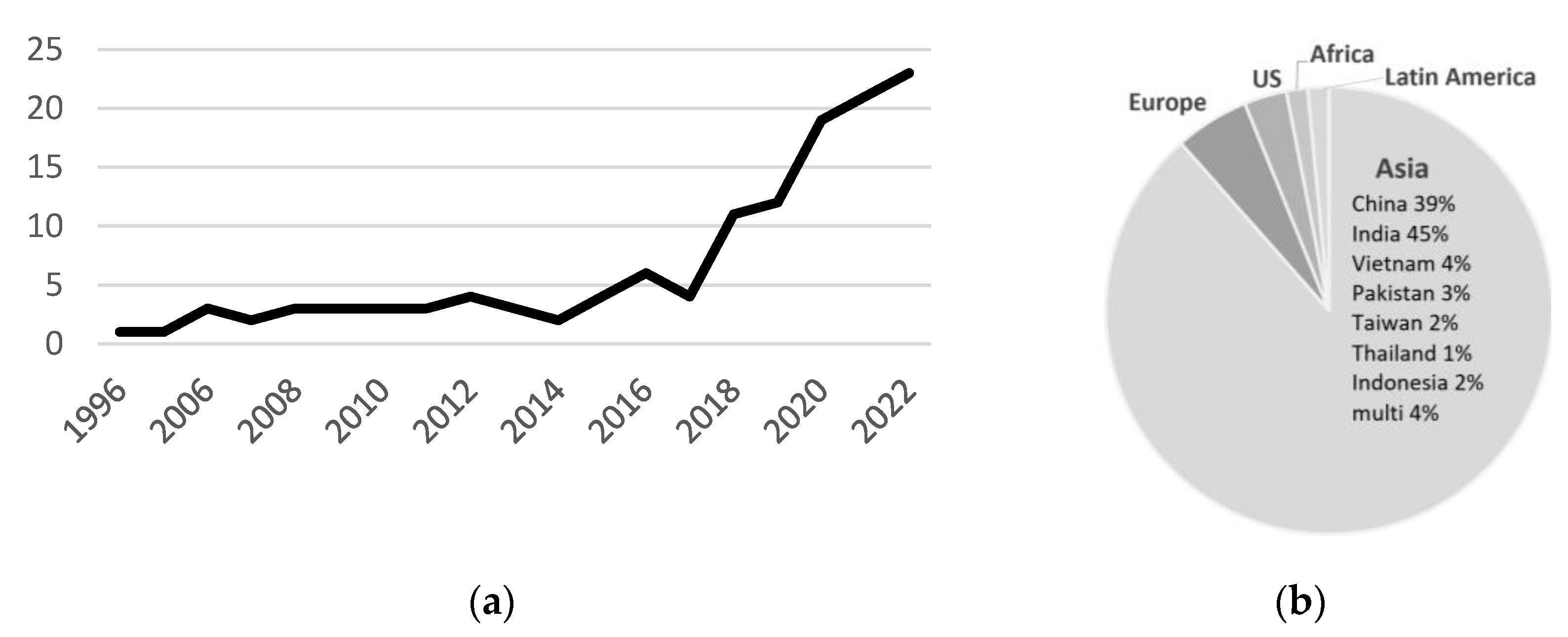
1.2. Literature Review

To assess the prevalence of these five pitfalls in studies of CRB using remotely sensed data and to identify strategies used in the literature to overcome them, we conducted a search on the ISI Web of Knowledge for publications with the keywords “crop/residue/straw/stubble”, “burn*”, and “remote sensing/satellite/earth observation”. Articles were included in the final set of papers if the authors made firsthand use of at least one remote sensor or sensor-derived product to estimate the extent, patterns, or impacts of crop burning. This keyword search returned 172 articles, of which 136 used a remote sensor/product firsthand (Table S1). Publications on this topic were fairly constant from 1996 to 2015 and have steadily increased since 2015 (Figure 1a).

Geographically, the literature is dominated by studies from Asia, particularly China and India (Figure 1b), and focuses mostly on rice and wheat burning. Studies cover all continents, however, indicating that CRB is a global issue. Of the 136 studies, 14 use satellite data only to measure atmospheric properties for emissions or pollution estimates. The 122 studies that use satellite data to estimate occurrences of fires themselves rely mostly on MODIS products (

Table 1. Sensors/products used to estimate crop burning in the literature.

Sensor/Product	#Studies a	Res (m)	Revisit	Available
MODIS_BurnedArea	25	500	daily	2000–present
MODIS_ActiveFire	65	1000	daily	2012–present
MODIS_custom	4	500	daily	2000–present
VIIRS_ActiveFire	16	375	daily	2012–present
Landsat	6	30	8–16 days	1982–present
Himawari-8	4	2000	10 min	2014–present
Sentinel-2	3	10–30	7 days (2017)	2015–present
Sentinel-1	3	10	12 days	2014–present
AWiFS	2	56	5 days	2003–present
LISS-3	2	24	24 days	2003–present
Formosat-2	2	2–8	daily c	2004–present
AVHRR	1	1100	daily	1981–present
PlanetScope	4 b	3	daily—7 days d	2017–present
composite products
Fire CCI (MODIS)	2	250	daily	1982–2019
L3JRC (SPOT)	2	1000	daily	2000–2007
GBA2000 (SPOT)	1	1000	daily	2000

^a a study can use more than one sensor/product. ^b All use PlanetScope to validate a model based on another sensor. ^c daily only if commissioned; very few images are typically available. ^d multiple smallsats can provide daily revisits, but coverage varies (see Section 3.1).

). Over half of the studies use a MODIS active fire product (MOD14/MYD14/MCD14ML), while about 20% use a MODIS burned area product (MCD64A1 or MCD45A1) and 3% use a different MODIS product. Following MODIS, the VIIRS active fire dataset is the most frequently used, appearing in over 13% of studies. Estimates of CRB in the literature differ drastically, even for the same area and time period. The authors attribute this difficulty in quantifying CRB mostly to Pitfall 1: the coarse spatial resolution of MODIS and VIIRS makes it difficult to assign quantitative values to burned areas, as well as to Pitfalls 2 and 3: the products used are most effective in detecting larger, longer-lived fires and fires with characteristic vegetation changes. The VIIRS active fire product provides an improvement in spatial resolution compared to its predecessor, the MODIS fire product, yet even after it became available in 2012, more studies continued to use MODIS active fire products compared to VIIRS (52 vs. 16).

Pitfalls 4 and 5 are very common in the current literature. Only one-quarter of studies that use sample data to train or validate a model of CRB include data from unburned classes, while the remaining three quarters fall into Pitfall 4 (inappropriate comparison category). Only 16 of the 122 studies that use remotely sensed data to estimate the extent or patterns of CRB contain data with which to validate burn mapping, thus underscoring the prevalence of Pitfall 5 (inadequate accuracy assessment). Among those 16, the quality of validation data varies: Nine validation sets are constructed from other remotely sensed data (2 Sentinel, 4 PlanetScope, 1 VHR, 2 GF-1), while seven use ground-based data. Of those seven, two use household surveys, and only five use plots visited on the ground. Where ground plots are used, the sample size ranges from 26 points for a two-class model [45] to 116 points for a six-class model [46]. Several additional studies have ground data for air quality measures serving as dependent variables but not for the burn measures used to quantify impacts or mitigation effects.

2. Materials and Methods

To illustrate particular issues that are inherent in CRB mapping, we provide an analysis of CRB detection using products with different spatial and temporal resolutions. Having noted the prevalence of MODIS and VIIRS-based products in the literature, we provide a comparison of estimates from these products to estimates from sensors with higher spatial resolution to illustrate Pitfall 1 (inadequate spatial resolution). Given the general agreement in the recent literature that products with low spatial resolution do not provide accurate estimates of CRB, however, our focus here is on pitfalls likely to be encountered using alternative approaches. In particular, we focus on common approaches using PlanetScope, Sentinel-2, and Landsat data and explore the effect of Pitfall 2 (inadequate temporal resolution) in these higher spatial resolution products while navigating Pitfall 3 (ill-fit signals) and Pitfall 4 (improper comparison groups).

We take advantage of a carefully collected ground dataset of both burned and unburned fields (Section 2.1) to assess estimates produced from other methods while elucidating both Pitfall 4 (improper comparison group) and Pitfall 5 (inadequate accuracy assessment). Despite having some ground data, our goal, as with any remote sensing analysis, is to classify locations where the status is not known from the ground. PlanetScope imagery, with a spatial resolution of three meters and an average temporal resolution of less than two days, can be an ideal sensor for CRB mapping. However, PlanetScope has some disadvantages compared to the more popular Landsat and Sentinel-2 products in that it is not freely available for public use and has a lower spectral resolution that only covers visible and near-infrared portions of the spectrum. While Sentinel-2 and Landsat products offer data on the mid- and short-wave infrared bands that can be useful for burn mapping, their lower temporal resolution (weekly to biweekly) can be problematic if it results in missed burn observations. With all products, actual gaps due to clouds, smoke, or other abnormalities can alter the temporal resolution and reduce quality.

To explore the consequences of gaps in imagery, we first conduct a separability analysis to estimate the detection window during which the burn signal can be reliably perceived following a burn event (Section 2.3.1). We then identify whether gaps exceeding this observation window exist in available imagery from each sensor (Section 2.3.2) and select a subset of our study area that represents the best-case scenario for burn detection based on the smallest nominal gap in PlanetScope imagery. This process allows us to locate the subset of our study area where we can produce the best-case representation of burning from all the imagery available to us. The tools we developed to determine minimum observation windows and quickly summarize temporal gaps in available imagery over a study area are available at https://github.com/klwalker-sb/cropburn, accessed on 8 January 2024.

Within this subset where the most available imagery coincides with a portion of our ground data for validation, we create a best-case model of CRB based on satellite imagery by manually digitizing observable burn scars from every available image, as described in Section 2.3.3. While this method is too labor-intensive for most modeling endeavors, it allows us to focus on the five pitfalls discussed here while putting aside considerations of how other modelling choices might affect outputs. Although our manually digitized dataset is used here to create a best-case model of burning for each sensor to compare to each other and to our ground data, we note that this approach is commonly used as a standalone validation method when ground data are not available. We compare results from our digitized model to our ground data to highlight the issue of relying on digitized data for validation when there are gaps in observations (Pitfall 5 × Pitfall 2).

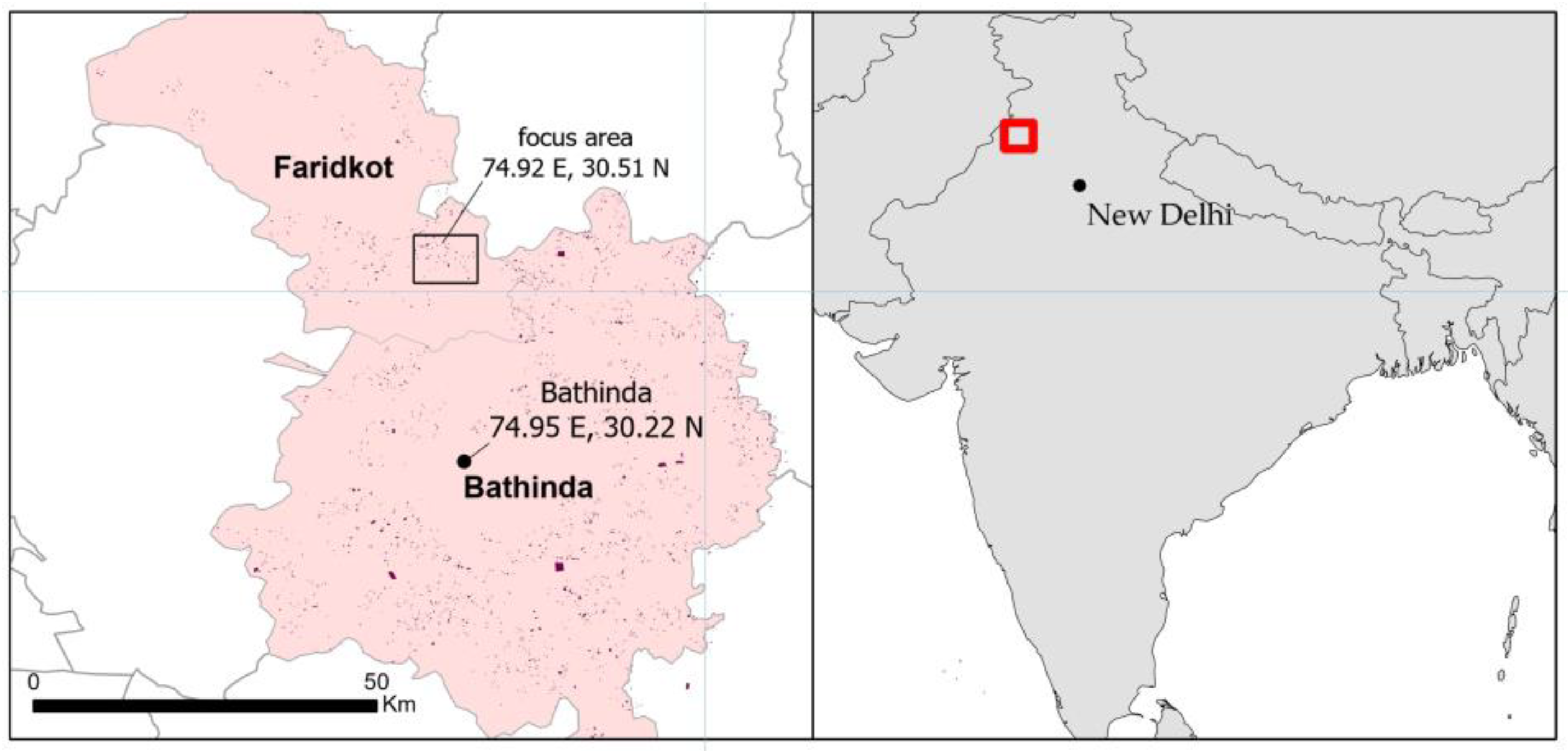
2.1. Validation Data from the Ground

Data used for accuracy assessment come from ground-level measures that were collected in 2019 as part of a study conducted in two districts in Punjab State, India (Figure 2). These data consist of irrigated rice plots in which stubble is normally burned post-monsoon season (between October and the beginning of the winter planting season in December) but were not all burned because farmers were participating in a randomized control trial in which some were paid to not burn [26]. Burning outcomes (labels) were collected for 240 unburned and 441 burned plots. Unburned plots were known to be unburned because participants needed to request a monitoring visit before tilling their field to demonstrate that it had not been burned (see [26] for additional detail). Plots were labeled as burned if signs of burning were discovered during this visit or a random spot check during the season. The plots in the area are small, with an average size of 1.4 ha and a median of 0.9 ha.

2.2. Imagery and Products

We selected an area within our ground study area in Punjab with the most PlanetScope observations and downloaded all imagery from the 2019 winter burn season (10 October to 20 December) as 4-band (B/G/R/Nir) surface reflectance images with harmonization applied [47]. For the same area and time period, we also downloaded all Sentinel-2 images from the European Space Agency’s Copernicus Data Hub; Landsat 7 and 8 images, MODIS burned area product (MOD64A1), and VIIRS burned area product from the U.S. Geological Service’s Earth Explorer; and MODIS and VIIRS active fire products from NASA FIRMS. Aside from the PlanetScope data, which was accessed under a paid academic license, all other data products were free.

2.3. Analysis Methods

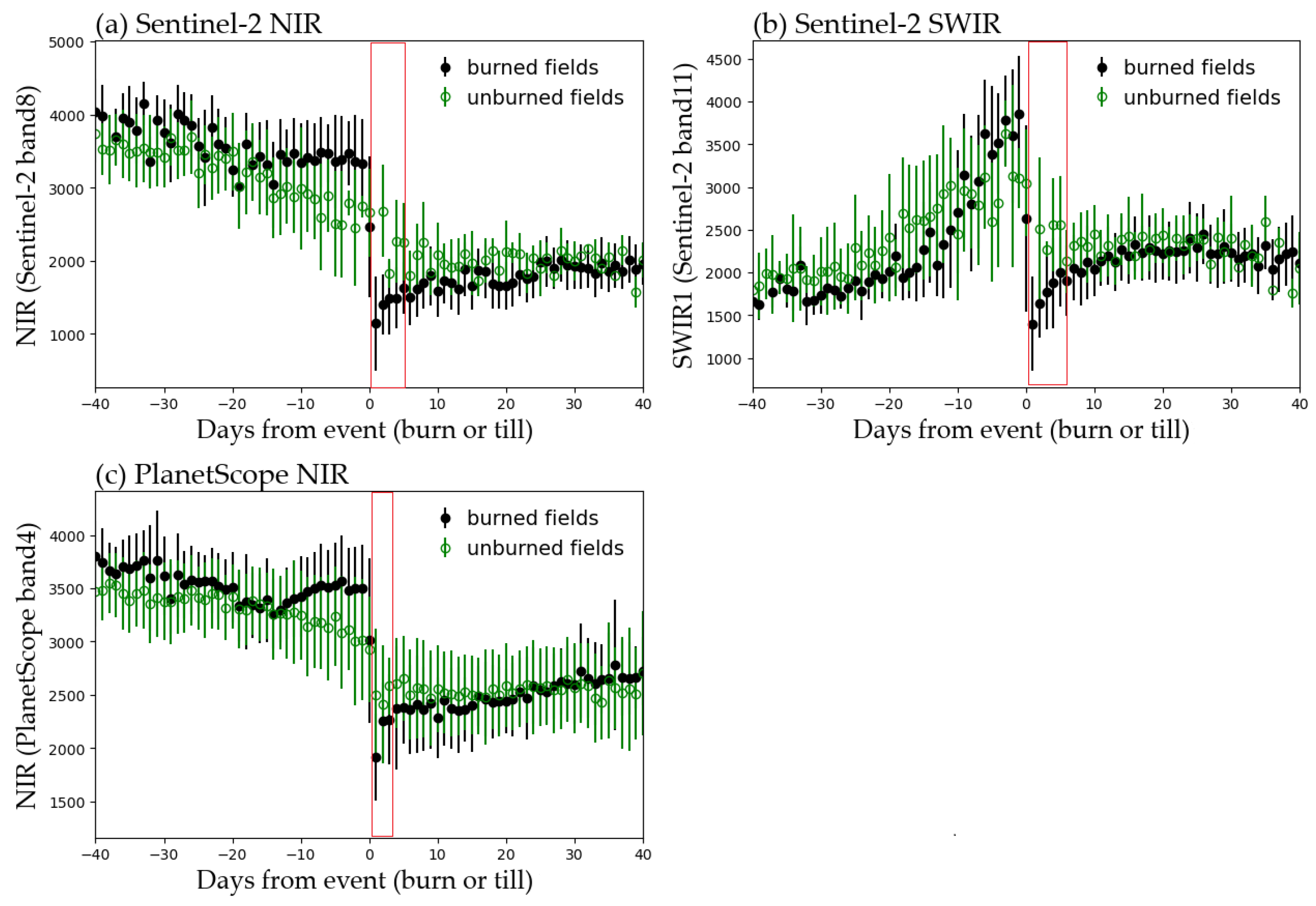
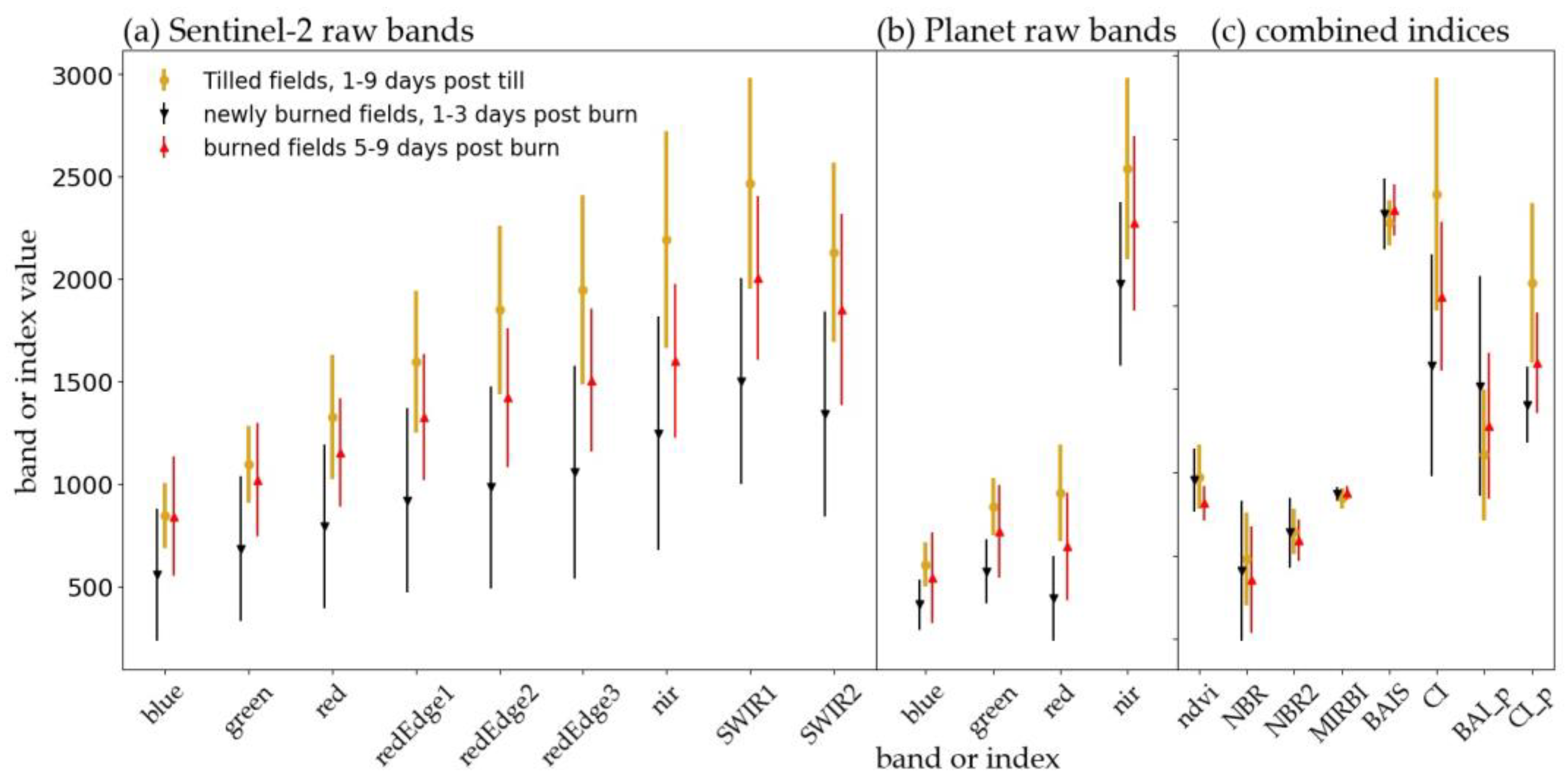
2.3.1. Separability Analysis and Signal-to-Noise Ratio

We evaluated the ability of individual bands as well as the most common spectral indices in the burn mapping literature to separate between burned and unburned areas and thus avoid Pitfall 3 (ill-fit signals), using visual interpretation of signals as well as the parametric M-statistic [48]: M = (μ_a − μ_b)/(σ_a − σ_b) where μ is the class mean, σ is the standard deviation, and a and b are the two classes, unburned and burned. An M-statistic above one suggests reasonable separability, although scores closer to two are desirable if minimizing errors of commission is a priority. We first conducted a preliminary separability analysis in the context of a pre-/post-burned matched analysis common to burn mapping for wildfires [49] to filter out the weakest performers. In the context of CRB, using this type of analysis alone leads to Pitfall 4, since all crops undergo a sharp change in vegetation around the time of harvesting and burning/tilling. For a separability analysis more appropriate to CRB, we compared burned rice paddy fields to rice paddy fields that were known to have been tilled in the same period but not burned, based on our ground data.

We conducted separability analyses with data from all datasets available to us that might provide, in combination, adequate spatial and temporal resolution: PlanetScope, Landsat, and Sentinel-2. Indices tested include NBR and other vegetation-based burn indices commonly used to map wildfires, in addition to burn scar and char indices specifically designed to map CRB (

Table 2. Indices used for separability analysis.

Indices without SWIR Band (Can Use with PlanetScope)
Normalized Difference Vegetation Index (NDVI)	$S\ast \frac{NIR-Red}{NIR+Red}$
Burn Area Index (BAI)	$\frac{S/100}{\left({0.06-NIR)}^2+{(0.1-Red)}^2\right) }$
Char Index (CI)	$S/10\ast (Blue+Green+Red+$ $15\ast Max(\left|Blue-Green\right|,|Blue-Red|,\left|Red-Green\right|))$
Indices with SWIR band (Sentinel and Landsat only)
Normalized Burn Index (NBR)	$S\ast \frac{NIR-SWIR2}{NIR+SWIR2}$
Normalized Burn Index 2 (NBR2)	$S\ast \frac{SWIR1-SWIR2}{SWIR1+SWIR2}$
Mid Infrared Bispectral Index (MIRBI)	$S/10\ast (10\ast SWIR2-9.8\ast SWIR1+2)$
Burn Scar Index (BSI)	$S\ast \frac{SWIR2-Red}{(SWIR2+Red)({Green}^2+{Red}^2+{NIR}^2)}$
Burn Area Indexfor Sentinel (BAI_S)	$S\ast \left(1-\sqrt{\frac{RedEdge2\ast RedEdge3\ast NIR }{Red}}\right) \ast \left(1+\frac{SWIR2-NIR}{\sqrt{SWIR2+NIR}}\right)$

S is a scale factor by which all bands are divided prior to calculation. In this study, all bands are from surface reflectance data (ranging from 0–10,000), thus S = 10,000.

). For each band and index (x) tested, we also calculated Δx = x_(t+1) − x_(t) to isolate changes. Given the prevalence of NBR and other vegetation-based indices in burn mapping, all were included in the initial analysis for comparison. As discussed above in Pitfall 3, however, the lesser-used char indices were expected to perform better for the task of detecting CRB.

As also discussed in Pitfall 3, accurate classification of CRB depends on a signal capable of separating burned plots from unburned, tilled plots despite noise in the imagery caused by differences in atmospheric and viewing conditions. Bands with longer wavelengths are generally less sensitive to noise, which is one reason that short-wave and mid-infrared bands are often used in indices. While multi-band ratios often reduce noise, the effectiveness of this tactic relies on the signal having one band that changes more than another band. We compared the bands/indices with the highest separability scores to the time-series signature of the stacked dataset to determine whether a ratioed index can accentuate that signal and the index’s ability to overcome noise in the data.

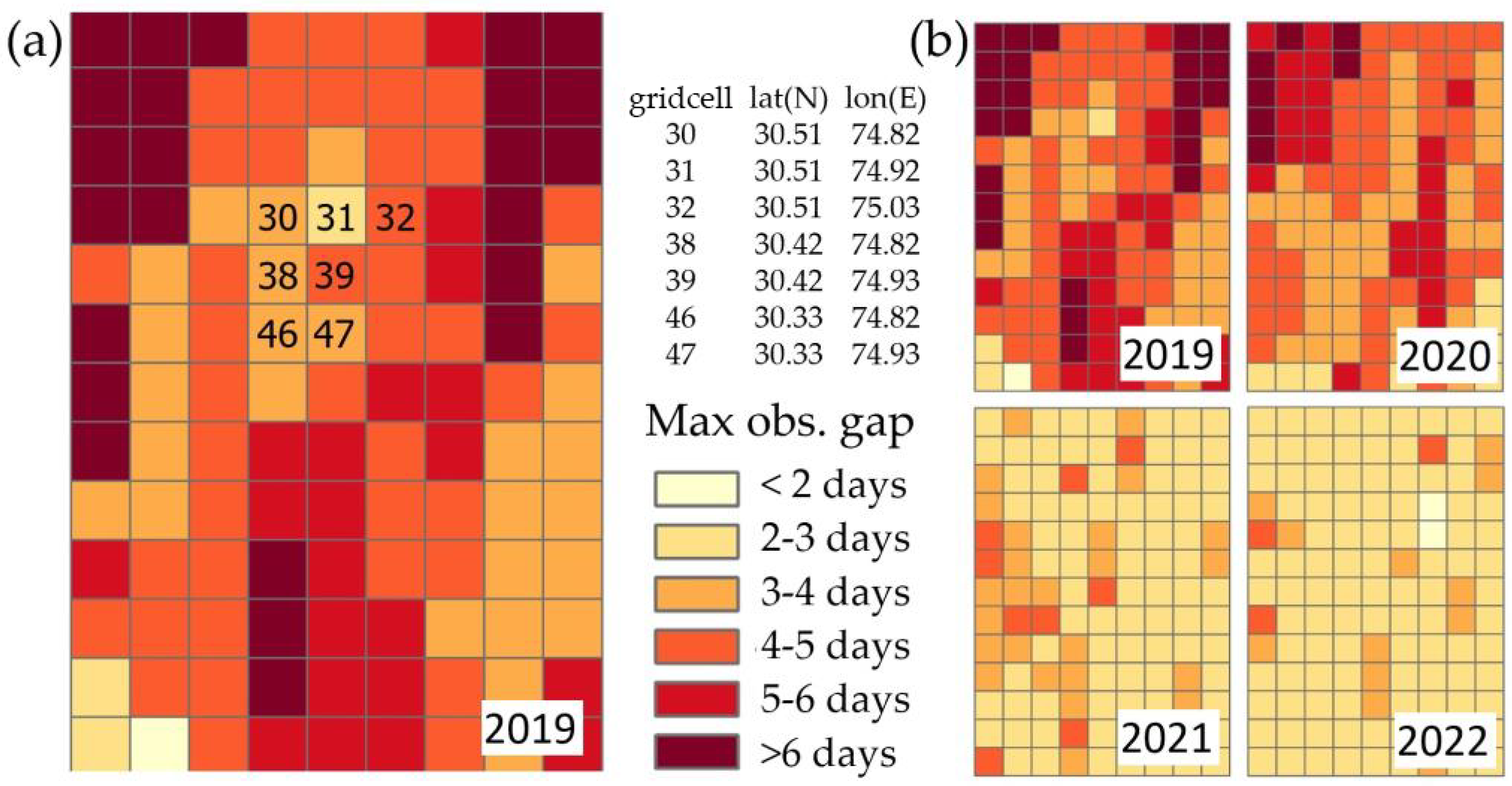
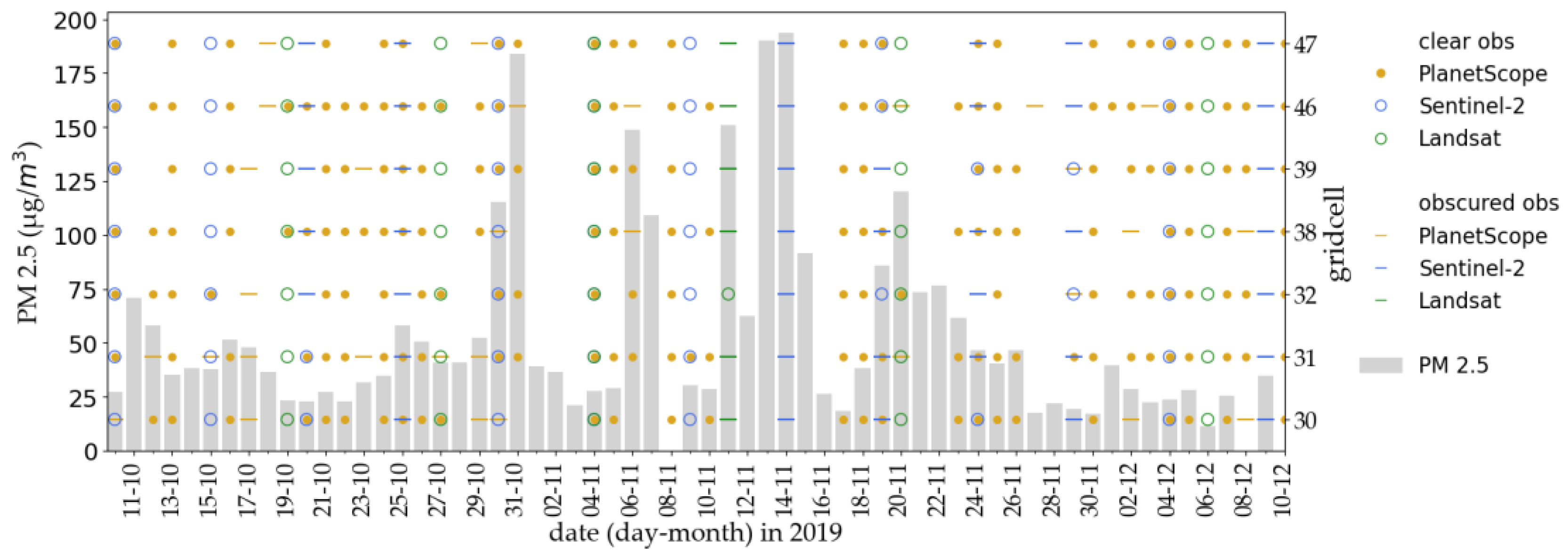
2.3.2. Estimating Detection Window and Observation Gaps

Accurate quantification of burning in remotely sensed data requires both a strong signal to distinguish burning as well as an adequate frequency of observations to capture all burn events and avoid Pitfall 2 (inadequate temporal resolution). The duration of the signal [50] compared to the background (tilled soil, in this case) determines adequate temporal resolution. To assess this detection window, we matched our ground data of burned plots to burn observations in PlanetScope imagery and retained those where we could confidently determine the date of the burn event within two days, meaning that a plot had a clear not-burned observation followed by a burned observation no more than two days later. Comparing this set to tilled plots in the separability analyses described in Section 2.3.1, we tested the temporal robustness of the signal by observing plots at increasing time spans since the burn event.

With the targeted detection window in mind, we assessed the temporal resolution of the products to determine whether any location in our study area had adequate temporal coverage to detect all burn events. We gridded our study area into 100 km² cells and queried the respective data repositories for the centroid of each cell to determine the average and maximum temporal gaps in the imagery. This allowed us to identify the cell with the best available imagery. For this cell as well as six surrounding cells that met our criteria of reasonable coverage of imagery as well as some ground data with which to assess model accuracy, we downloaded all PlanetScope, Sentinel-2, and Landsat data and applied the cloud masks supplied with the imagery to determine the actual observation gaps.

To contextualize observation gaps and whether they occurred during peak periods of burning, we looked at hourly pollution data from ground station observations maintained by India’s Central Pollution Control Board (https://app.cpcbccr.com, accessed on 8 January 2024). (Due to temporary site maintenance, we downloaded the data secondhand from [51], accessed on 20 November 2023). As smoke plumes observed in PlanetScope imagery were typically blowing toward the S or SE, consistent with other studies in the region [52], we used data from the Bathinda station, 32 km SE of our focal area (Figure 2). We focused on records of fine particulate matter (PM_2.5), as it has been shown to be particularly correlated with CRB [2,12]. Heavy CRB activity under unfavorable weather conditions is known to cause thick haze that can obscure optical imagery [53,54].

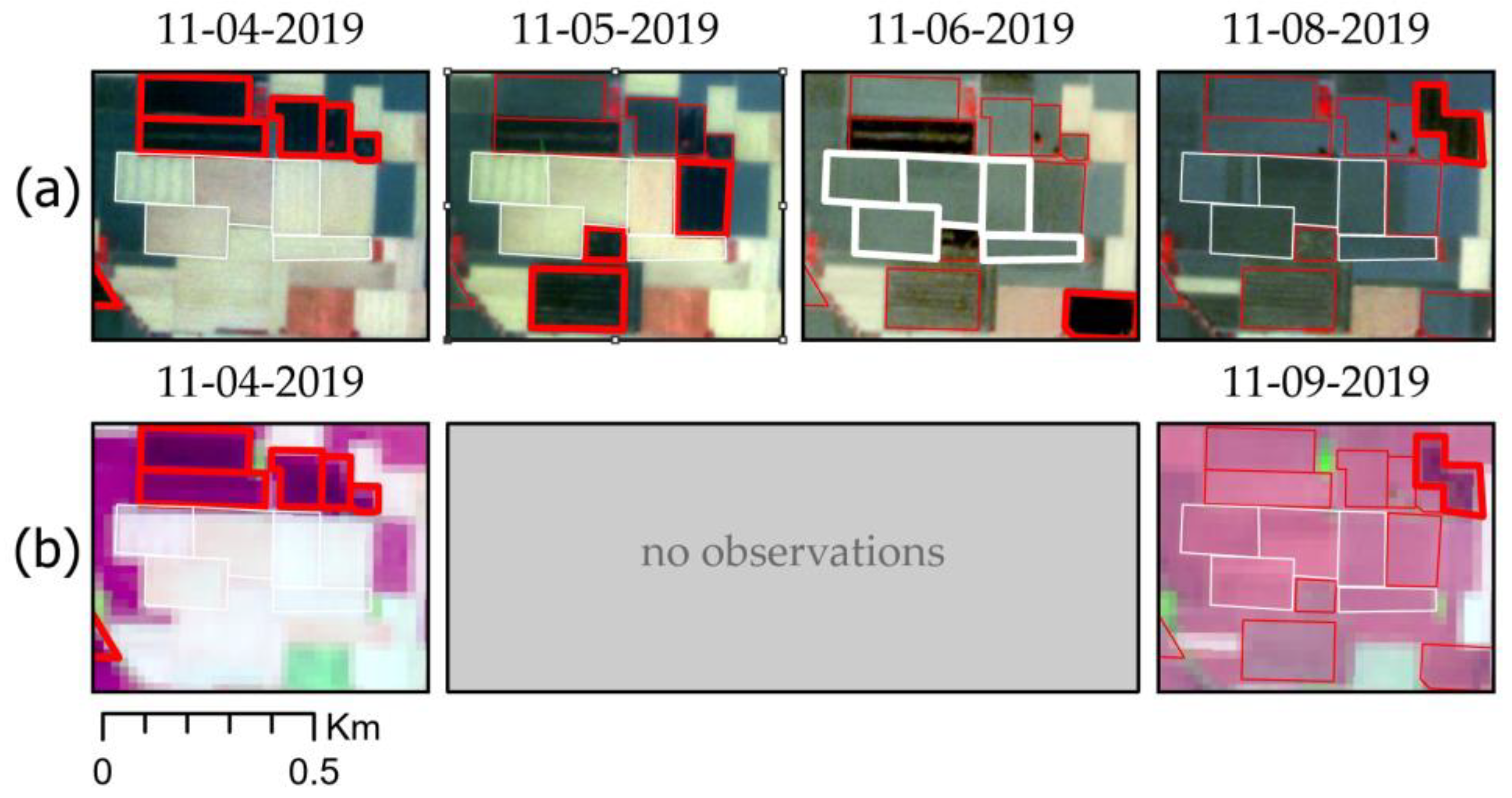
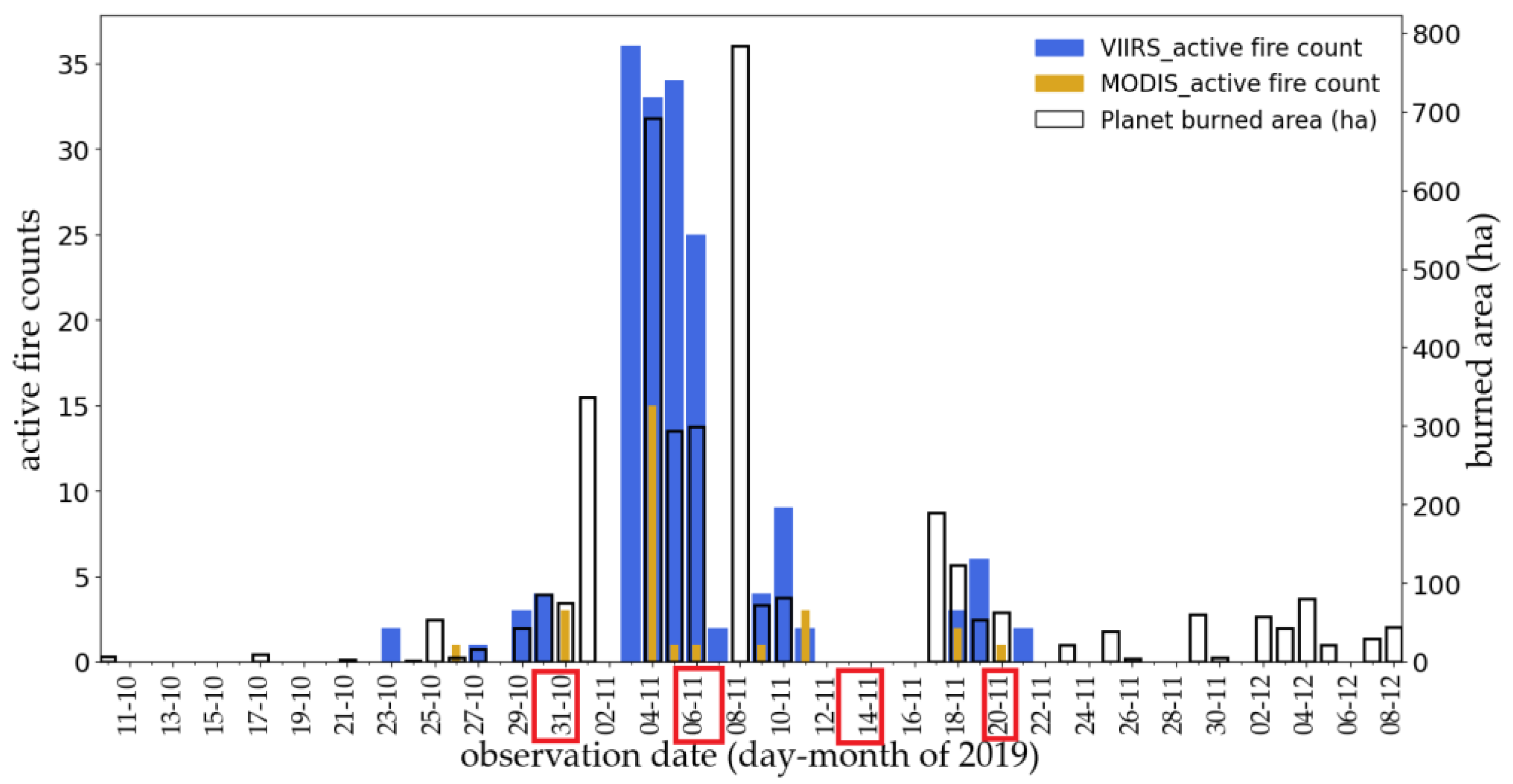
2.3.3. Burn Scar Time Series Dataset and Effect of Observation Gaps on Estimates of CRB

For accurate quantification of CRB and avoidance of Pitfalls 1 and 2, both adequate spatial and temporal resolution are required. We explored the effect of products with different resolutions on CRB estimates by constructing a dataset of all burn events observed at the highest spatial and temporal resolution available and comparing this to similar analyses with datasets at lower resolutions and with our ground validation data. For the best-case focus area selected by the process described in Section 2.3.2, we constructed the best possible model of burned area for the 2019 winter burn season by extracting burned plots from each individual image using AI-assisted manual digitization. Manual digitization is a common method to create training data for burned areas and is considered a good validation tool as long as the imagery used for validation has a higher resolution than the imagery the model is built on [43]. Although there is some degree of subjectivity in selecting thresholds for burn scar labeling, this method is generally more reliable than machine-learning models when imagery is noisy because the human eye is good at seeing past spectral differences and haze to select the appropriate thresholds for a given context.

Our digitization protocol involved opening each image in ArcGIS Pro as a false color composite (R: SWIR2, G: NIR, B: red for Sentinel-2 and Landsat images and R: NIR, G: red, B: green for PlanetScope images) and using the segmentation tool based on Segment Anything (SAM) with a minimum mapping unit of 900 m² to convert the image into polygons. We used visual inspection to select thresholding values specific to each image to extract the burned areas, and then manually digitized any polygons missed due to haze and erased any areas erroneously identified as burned due to shadows or clouds. We aggregated the results from individual images into a single dataset of burned fields for the season for each sensor. To limit the analysis to potential rice fields, areas with low NDVI in a clear preharvest (August) Sentinel-2 image were masked following the methods of Deshpande et al. [55]. A preliminary analysis of our field data revealed pre-harvest NDVI for rice paddies to be quite variable (Figure S1), and little area could be safely masked beyond built areas. A conservative threshold of NDVI < 6000 was selected for the mask based on this analysis. Additional urban, water, tree, and tree-shadow masks were created with the segmentation tool and retouched manually. We compared aggregated estimates for each sensor to each other at each cell. We also matched each daily burn scar dataset with the MODIS and VIIRS active fire products to assess the proportion detected by those products. Finally, we applied the labeled ground data available for each cell to the burn/no burn classification at each corresponding location to assess model performance in terms of missed events or false alarms and adjusted estimates accordingly.

3. Results

3.1. Separability, Signal-to-Noise Ratio, and Detection Window

Based on visual inspection of the imagery, burn scars are obvious in both PlanetScope and Sentinel-2 images if observed within a day. After two or three days, however, burned plots are very difficult to distinguish from unburned plots. This is illustrated in Figure 3, where PlanetScope and Sentinel-2 images are compared with burned plots outlined in red, and unburned plots outlined in white. In these images, charred plots stand out when observed within 24 h of the burn event but blend in with unburned, tilled plots within days. Analyses where imagery from Sentinel-2 or other sensors with multi-day gaps are the only data source will thus likely miss many burn events (Figure 3b).

These qualitative observations are supported by more detailed analyses of the NIR and SWIR signatures of plots with known burn dates. Figure 4 shows the temporal changes of the NIR (Sentinel-2 and PlanetScope) and SWIR1 (Sentinel-2) bands across time with respect to the burning/tilling event (day 0).

All of the panels in Figure 4 indicate that the NIR and SWIR signals drop sharply at the point of burning, but a similar drop also occurs with unburned, tilled plots. The signals do reach a lower minimum with burning than with just tilling, but this quickly increases, and the ability to separate burned vs. tilled plots dissipates within days. Without data from tilled plots, the abrupt and persistent change in signal might lead to the conclusion that burning has high separability and can be mapped with high accuracy based on these bands alone. This, however, would be an example of Pitfall 4. It is, in fact, tilling that has high separability; pre- and post-tilled plots can be separated with high accuracy using the NIR and SWIR bands, but determining whether they were burned prior to tilling is less straightforward. Plots known to be tilled but not burned show a similar signal to that of the burned plots, and observations close to the event with little noise are required to determine whether burning occurred.

For pre- and post-burned plots, all bands and indices tested had an M-statistic well above the standard threshold of one, often approaching two, that lasted up to two weeks after the burn event (Figure S2). However, when comparing burned plots to unburned, tilled plots, only SWIR, NIR, and the char index [37] provided adequate separability for observations more than two to three days after the burn event, and this quickly dissipated after five days. The brevity of the separability is further illustrated in Figure 5, which shows the overlap in standard deviations of signal values for Sentinel-2 and PlanetScope bands for tilled plots with plots burned one to three days and five to nine days prior to the observation.

Figure 5a,b show that most individual bands can effectively separate burned plots from tilled plots if the burning has occurred within three days but will introduce much confusion if the event is more than five days old. In contrast to single bands, all ratioed indices have low separability, even for observations right after the burn event (Figure 5c). This is because all bands change similarly in response to charring, as seen in Figure 5a,b. The non-ratioed char index is the only index that performed well, slightly outperforming the individual SWIR and NIR bands (however, not enough for us to judge the extra work in using it worthwhile for the purposes of our burned area analysis). This exercise demonstrates why using ratioed indices to map CRB is likely to result in Pitfall 3 (ill-fit signals) for indices that largely target vegetation change, such as NDVI and NBR, as well as those that more specifically target burning, such as the Burned Area Index (BAI).

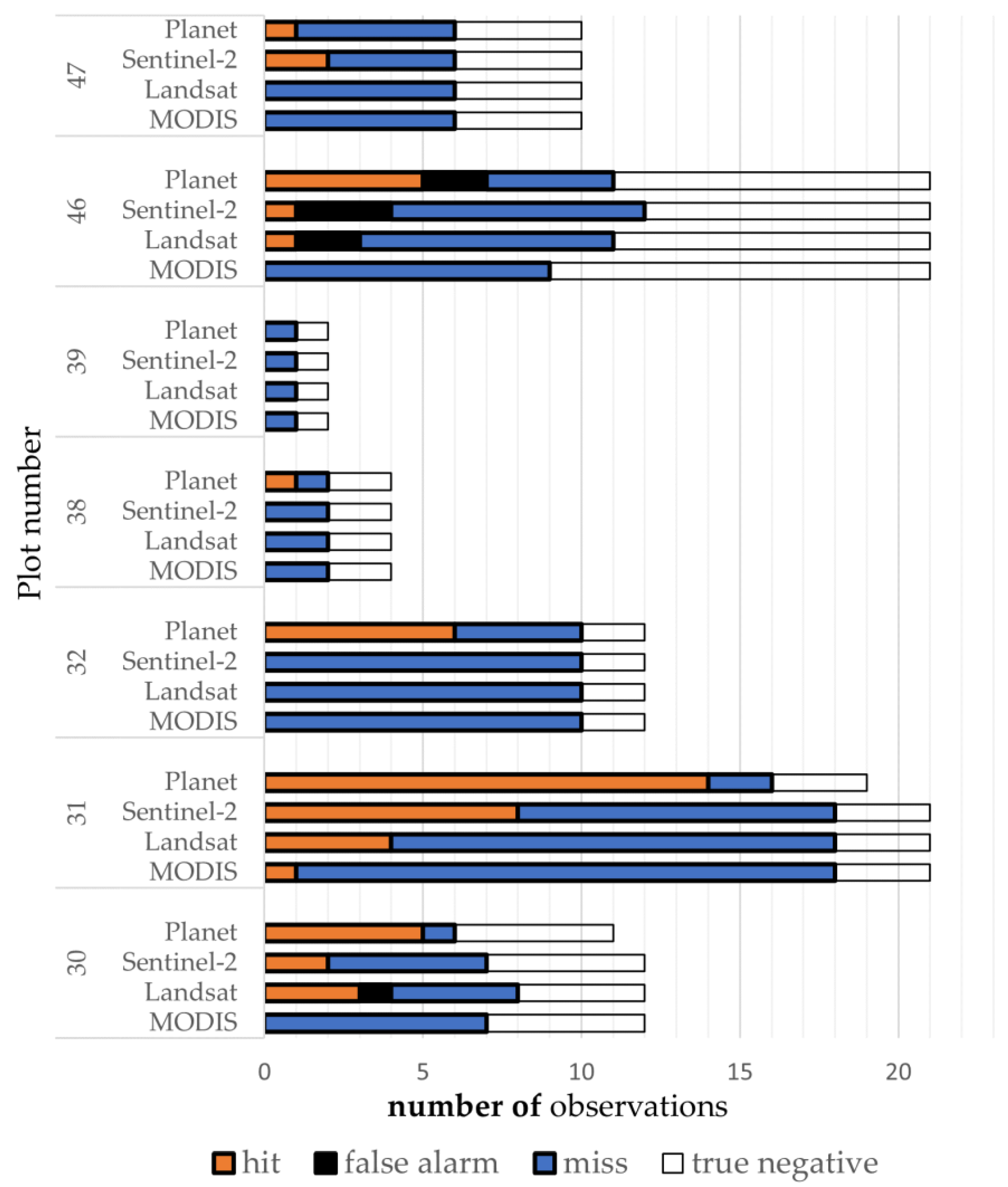
3.2. Observational Gaps

While the average temporal frequency is nominally one to two days for PlanetScope and five to ten days for Sentinel-2, much larger gaps can occur in the time series due to clouds or other abnormalities. To locate areas with the smallest gaps for subsequent analyses, we first used our gridded gap tool, presented in the linked code, to estimate gaps resulting from missing images. Figure 6a shows the result of this gridded gap analysis, with darker colors indicating areas with longer gaps in the available PlanetScope imagery. Most of our study area is revealed to have gaps in available imagery of more than three days, often exceeding six days, in 2019. While the gridded gap tool accounts for overall cloud cover by excluding images with cloud cover exceeding a set threshold, it does not account for local clouds. In an analysis using imagery with cloud masks applied across the full study area [21], we found an average temporal gap of 8.4 days at some point during the burn season for PlanetScope and 13 days for Sentinel-2. Given the two-day observational window for burn events discussed in Section 3.1, these gaps will likely result in missed events and thus Pitfall 2. For the burned area analysis that follows, we tried to minimize the effects of Pitfall 2 by selecting one of two grid cells in our area found to have gaps of less than three days as our focal point (cell no. 31).

The issue with observational gaps is at least partially created by CRB itself. Figure 7 shows the presence of clear observations for Landsat and Sentinel-2, in addition to PlanetScope, at the centroid of each of the seven cells identified as the focal area in Figure 6. The gray bars show PM_2.5 concentrations in nearby Bathinda. All three sensors have large gaps around the same period. These observational blackouts generally follow days with high PM_2.5, suggesting that they are primarily connected to the large-scale occurrence of CRB. The short detection window discussed in Section 3.1 suggests that the many burn events occurring during these periods will not be observed in optical imagery, resulting in potentially large omission errors for measurements relying on such sensors.

Missing observations during periods of high smoke are common in active fire products as well. Figure 8 shows active fire counts from VIIRS and MODIS products compared to our burned area analysis with PlanetScope imagery (discussed in Section 3.3), with red boxes indicating periods of heavy smoke (PM_2.5 above 100 mμ/m³). These smoky periods often correspond to periods with low active fire counts. Given that the PM_2.5 measurements are recorded 32 km SE, it is possible that the smoke originates from outside of the area to which the satellite data correspond (for example, the area NW of our focal area, where larger gaps in PlanetScope observations (Figure 6) could indicate even more heavy burn days). However, Figure 8 shows that large areas of burn scars are often detected in PlanetScope observations immediately following periods of heavy smoke. These fresh burn scars do not always have corresponding active fire counts during the heavy smoke days, thus suggesting missed observations in the active fire data.

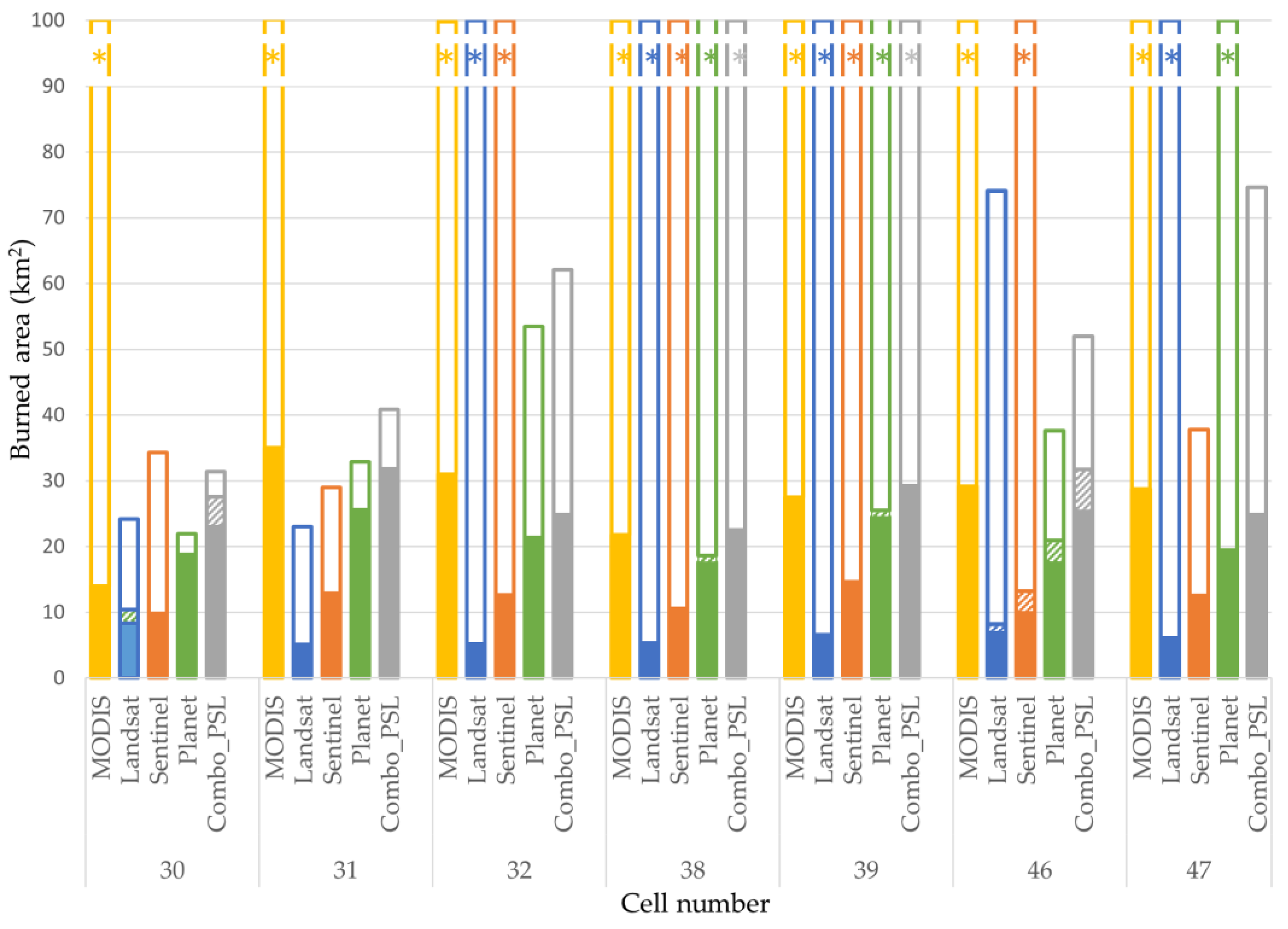
3.3. Effect of Resolution on Burned Area Estimates

Where CRB is prominent, burned-area estimates increase with increasing temporal resolution. Figure 9 shows the 2019 winter burned-area estimates for the seven focal cells based on manual digitization of all observable burn scars from PlanetScope, Sentinel-2, and Landsat imagery. Estimates are consistently largest on the sensor with the highest temporal resolution (PlanetScope) and decrease with decreasing temporal resolution. In Figure 10, which presents the accuracy assessment of these results based on our ground data, more blue misses (missed burn events) compared to orange hits (correctly identified burn events) are observed as temporal resolution decreases. This is especially notable for grid cell 31, which has both the most ground data and PlanetScope observations. Overall, 35% of known burn events were missed with PlanetScope (but only 11% in cell 31), while 72% were missed with Sentinel-2 and 86% were missed with Landsat, thus demonstrating the prevalence of Pitfall 2 (inadequate temporal frequency) with datasets of high spatial resolution. Some observations missed in PlanetScope can be filled with Sentinel and Landsat observations, such that our combo dataset captures the most burned area (but still misses over 30% of known burn events). Generally, however, observations are missing for all sensors around the same period, as discussed in Section 3.2. Based on this observation, even sensors with optimal temporal resolution during normal periods would likely miss burn events due to heavy smoke.

While Figure 9 shows that data from different sensors results in different burned area estimates, Figure 11 shows the differing spatial distribution of burned area for four products for the same area (cell no. 31) and time period (2019 winter burn season). Spatial differences are especially notable with the MODIS burned area product, for which area estimates are very similar in magnitude to estimates from PlanetScope imagery (Figure 9), though spatial patterns differ substantially (Figure 11b vs. Figure 11a). Our ground data confirms the unreliability of the MODIS burned area product for estimating CRB at both plot and aggregate levels; only two of 64 of our burn labels from ground data were identified as burned in the MODIS dataset, thus making it impossible to even statistically adjust area estimates. Our findings are in line with other analyses, which have found 97% omission error for VIIRS and 100% omission error for MODIS data [20] and illustrate the consequences of Pitfall 1 (inadequate spatial resolution). This spatial inaccuracy is likely due to the fact that whole 500 m (25 ha) grid cells are flagged as burned or unburned in MODIS burned area products.

Unlike burned area products, active fire products allow for flexibility in determining the size of the burned area by assigning the size to each fire count. Despite this theoretical flexibility, Figure 8 shows that each VIIRS fire count would need to correspond to a full pixel (about 14 ha) for the magnitude of the burned area detected with the VIIRS active fire product to match the magnitude of the burned area we estimated with PlanetScope imagery (which Figure 9 shows is an underestimate of the actual burned area). Figure 8 also shows that the MODIS active fire product greatly underestimates the area, even if each fire count corresponds to a full 25 ha pixel of burned area. This supports findings by others (e.g., [2,39]) that many fires need to be burning at one time for a VIIRS fire event to be triggered. This is further corroborated by the lack of VIIRS observations at the end of the burn season (Figure 8), similar to findings by Jethva et al. [2] that events are less likely to be detected during times when they are sparser. Qualitatively, it is clear that MODIS and VIIRS-based products do not provide the same degree of spatial precision as PlanetScope and Sentinel-2 and result in misclassification of burning at the plot level. The spatial difference between the MODIS and VIIRS products and PlanetScope, shown in Figure 11, further illustrates Pitfall 1. The underestimation of burning by all products due to missed observations, as shown in Figure 8 and Figure 9, illustrates Pitfall 2.

4. Discussion

Mapping and quantifying CRB with remote sensing data is a difficult task due to the small size of burned plots, short duration of the signal prior to tilling, weak signal compared to tilled land, and high sensitivity to noise within and between images. Here we have identified and explored five pitfalls that frequently obstruct efforts to quantify CRB with remote sensing data. A search of the relevant literature uncovered 172 articles on remote sensing and CRB. While these articles make important contributions to measuring the extent and implications of CRB, all fall into one or more of the pitfalls.

The first four pitfalls result in errors, which could be evaluated and sometimes corrected for (in the case of coarse-scale estimates), but for the fact that almost all articles also fall into Pitfall 5 (lack of adequate accuracy assessment). Without a proper accuracy assessment, the scale of errors in these studies cannot be determined beyond the observation that the errors are generally found to be large for these pitfalls. The most common pitfalls, Pitfall 1 (inadequate spatial resolution) and Pitfall 2 (inadequate temporal resolution), generally result in errors of omission and gross underestimation of CRB [20], although local errors of commission are also common with burn products with low spatial resolution [20,45,56]. Pitfall 3 (mapping CRB with ill-fitted signals) leads to both errors of omission and commission. If the signal is based on vegetation change, errors of commission are likely. In an analysis of crop burning in the United States, McCarty et al. [45] note high rates of commission with image differencing using NBR (ΔNBR), likely because NBR is largely a measure of vegetative state. Burned area products that use similar vegetation indices, such as the MODIS and derived products, have high errors of commission in identifying much agricultural land as burned [57]. Pitfall 4 (mapping against the wrong comparison group) also leads to errors of commission, especially when labels from burned—but not unburned, tilled—fields are used to train a model to detect burning. A model based on such data will overclassify burning, while an accuracy assessment based on validation data with the wrong comparison group will overconfidently assess model performance, a common issue in the cases we reviewed.

In addition to measuring the accuracy of CRB mapping against the wrong comparison group (or without any labels for the unburned class) (Pitfalls 5 × 3), another common issue with the accuracy assessments that are presented in the literature is inadequate temporal resolution for the assessment itself (Pitfalls 5 × 2). If the objective is to quantify CRB or assess the accuracy of another product in quantifying CRB, burn and no-burn labels need to be accurately constructed by observing plots at all points in time (or using a ground-based validation method to observe tilling). Observing a point as unburned at single points in time provides little to no information about its ultimate treatment because it could be burned at an unobserved point. This need for regular observations through the full burn season is relevant for both ground-level and remotely sensed observations. While we advocate for ground data when possible, we acknowledge the difficulty in constructing a ground-based dataset where unburned plots are confirmed to be unburned throughout the whole burn season rather than just a single point in time. Remote sensing might offer a mechanism for full-season observation, but consideration of missed observations should be at the forefront of the analysis. Our findings that over one-third of our ground-validated CRB events were still missed in our most carefully constructed remote sensing dataset and that all sensors appear to be missing observations around the peak of the fire season suggest that extreme smoke will be a problem for most remote sensing analysis and should be a consideration for any validation based on optical remote sensing data.

Most accuracy assessments presented in the literature do not even attempt to cover the full burn season or all observations during the season. While validation sets are often of higher spatial resolution than the model being validated, in accordance with the recommended protocol, the same consideration is rarely applied to temporal resolution. For example, Padilla et al. [56] validated MODIS burned area maps using pre-post image pairs separated by about 32 days. While they report high errors of omission in the MODIS data, errors are likely even higher than reported due to the missing observations of CRB events in the validation set. Liu et al. [58] validated a model of CRB on wheat plots in China based on a single Landsat-8 image with a single Gaofen-1 image from the same day. While their 95% accuracy can provide a good check on the ability of the model to detect recently burned plots, it says little about the ability to measure CRB overall. While validating across a longer time series, Liu et al. [59] used the same Landsat imagery to build their model and validate it. Due to the long gaps between Landsat images and likely missed events, accuracy in quantifying CRB is almost certainly inflated. Deshpande et al. [55,60] constructed a careful validation set from PlanetScope to validate burned areas from Sentinel-2 but selected only images from the same acquisition date. The very low omission errors reported in their study reflect the ability to detect recently burned patches in Sentinel-2 images and validate their manual digitization approach for single-date classification, but say little about the ability of their Sentinel-2 model to quantify burning by detecting all burns through the season.

To accurately quantify CRB, remote sensing data must be at the spatial and temporal frequency required to capture all events and ensure that a lack of observed burning indicates that a burn event did not occur rather than that it was missed. To check whether a product provides adequate temporal coverage, we offer the gridded observation tool used in Figure 6. This is particularly useful during the planning stages of analysis to scan large areas and identify locations where conditions are ideal or inadequate for achieving the desired accuracy. To assess the likelihood of detecting the burn signal without introducing high errors of commission given the noise of the imagery, we propose an additional initial signal-to-noise test (Figure S3), provided in the same code repository. In our case, we found that the noise in PlanetScope outweighs the signal from any single band or ratioed index, thus leading to high errors when automated modeling is used (without calibrating burn thresholds for individual images). While this should serve as a cautionary flag, better fitting may be possible with multiple indices and a more complex model structure (see, for example, the random forest model described in Walker et al. [21] and Jack et al. [26] and the results in Deshpande et al. [55]. Alternatively, imagery could be better calibrated, or an image-by-image approach could be adopted such as the one used here for the PlanetScope dataset.

The pitfalls discussed here are general and ubiquitous to all types of CRB. Characteristics specific to a location or cropping system might raise other issues or lead to different details related to these pitfalls in ways not explored here. For example, Liu et al. [23] discuss challenges presented by fragmented burned areas and rough topography, which adds extra noise to the imagery. Similarly, Liu et al. [29] discuss the prevalence of partial burning in some areas; if residue is raked into a small area within the field prior to burning, the signal will be even more difficult to detect. The setting in Hall et al. [24], on the other hand, places lower demands on spatial resolution due to relatively large field sizes but encounters extra difficulty separating signals due to very black soil in the region (Ukraine).

Despite the pitfalls and errors that plague efforts to map CRB with remote sensing data, tools are increasingly becoming available to overcome these errors and produce better estimates of CRB. Smallsats, such as PlanetScope, offer ever-better temporal frequency that can help overcome observational gaps that hinder the construction of quality training and validation data. Since the time period of the study presented here, average observational gaps in PlanetScope imagery have decreased notably over our study area (Figure 6b). A similar analysis as the one presented here for a more recent year might produce more favorable results, though the problem of missing observations during the height of the burn season likely persists. Other types of remotely sensed data, such as radar or thermal, might help “see” through the smoke and fill in the gaps during the height of the burn season [61,62]. Along with the increasing availability of higher-resolution data and different types of sensors, continuing advances in machine learning and other computational methods can facilitate the processing of the large amounts of data required for such an endeavor.

Careful navigation of the five pitfalls discussed here can help improve the accuracy of estimates of CRB to improve emissions databases [24] and inform policy to reduce the occurrence of CRB. Burned area products provide a primary input into fire emission databases and atmospheric transport models; large omission errors thus have substantial downstream impacts on the emission databases and policy implications. Many potential policies to reduce the occurrence of CRB require effective (remote or in-person) monitoring to implement and evaluate [26,63,64,65]. Likewise, remote detection of CRB can help overcome technical and political economy barriers to the enforcement of policies banning CRB, such as those in effect but largely ignored in India and China [66,67].

References

1. World Health Organization. Overview of Methods to Assess Population Exposure to Ambient Air Pollution; World Health Organization: Geneva, Switzerland, 2023. [Google Scholar]
2. Jethva, H.; Chand, D.; Torres, O.; Gupta, P.; Lyapustin, A.; Patadia, F. Agricultural Burning and Air Quality over Northern India: A Synergistic Analysis using NASA’s A-train Satellite Data and Ground Measurements. Aerosol Air Qual. Res. 2018, 18, 1756–1773. [Google Scholar] [CrossRef]
3. Liu, T.; He, G.J.; Lau, A.K.H. Statistical evidence on the impact of agricultural straw burning on urban air quality in China. Sci. Total Environ. 2020, 711, 134633. [Google Scholar] [CrossRef]
4. Ashraf, M.F.; Ahmad, R.U.; Tareen, H.K. Worsening situation of smog in Pakistan: A tale of three cities. Ann. Med. Surg. 2022, 79, 103947. [Google Scholar] [CrossRef]
5. Chakrabarti, S.; Khan, M.T.K.; Avinash Roy, D.; Scott, S.P. Risk of acute respiratory infection from crop burning in India: Estimating disease burden and economic welfare from satellite and national health survey data for 250,000 persons (vol 48, pg. 1113, 2019). Int. J. Epidemiol. 2020, 49, 710–711. [Google Scholar] [CrossRef] [PubMed]
6. Cusworth, D.H.; Mickley, L.J.; Sulprizio, M.P.; Liu, T.J.; Marlier, M.E.; DeFries, R.S.; Guttikunda, S.K.; Gupta, P. Quantifying the influence of agricultural fires in northwest India on urban air pollution in Delhi, India. Environ. Res. Lett. 2018, 13, 044018. [Google Scholar] [CrossRef]
7. Day, M.; Pouliot, G.; Hunt, S.; Baker, K.R.; Beardsley, M.; Frost, G.; Mobley, D.; Simon, H.; Henderson, B.B.; Yelverton, T.; et al. Reflecting on progress since the 2005 NARSTO emissions inventory report. J. Air Waste Manag. Assoc. 2019, 69, 1023–1048. [Google Scholar] [CrossRef] [PubMed]
8. McDuffie, E.E.; Martin, R.V.; Spadaro, J.V.; Burnett, R.; Smith, S.J.; O’Rourke, P.; Hammer, M.S.; van Donkelaar, A.; Bindle, L.; Shah, V.; et al. Source sector and fuel contributions to ambient PM2.5 and attributable mortality across multiple spatial scales. Nat. Commun. 2021, 12, 3594. [Google Scholar] [CrossRef]
9. Rabha, S.; Saikia, B.K.; Singh, G.K.; Gupta, T. Meteorological Influence and Chemical Compositions of Atmospheric Particulate Matters in an Indian Urban Area. ACS Earth Space Chem. 2021, 5, 1686–1694. [Google Scholar] [CrossRef]
10. Ravindra, K.; Singh, T.; Mor, S. Emissions of air pollutants from primary crop residue burning in India and their mitigation strategies for cleaner emissions. J. Clean. Prod. 2019, 208, 261–273. [Google Scholar] [CrossRef]
11. Wang, L.L.; Jin, X.; Wang, Q.L.; Mao, H.Q.; Liu, Q.Y.; Weng, G.Q.; Wang, Y.S. Spatial and temporal variability of open biomass burning in Northeast China from 2003 to 2017. Atmos. Ocean. Sci. Lett. 2020, 13, 240–247. [Google Scholar] [CrossRef]
12. He, G.J.; Liu, T.; Zhou, M.G. Straw burning, PM2.5, and death: Evidence from China. J. Dev. Econ. 2020, 145, 102468. [Google Scholar] [CrossRef]
13. Jethva, H.; Torres, O.; Field, R.D.; Lyapustin, A.; Gautam, R.; Kayetha, V. Connecting Crop Productivity, Residue Fires, and Air Quality over Northern India. Sci. Rep. 2019, 9, 16594. [Google Scholar] [CrossRef] [PubMed]
14. Liu, T.; Crowley, M.A. Detection and impacts of tiling artifacts in MODIS burned area classification. IOP SciNotes 2021, 2, 014003. [Google Scholar] [CrossRef]
15. Badarinath, K.V.S.; Chand, T.R.K.; Prasad, V.K. Agriculture crop residue burning in the Indo-Gangetic Plains-A study using IRS-P6 AWiFS satellite data. Curr. Sci. 2006, 91, 1085–1089. [Google Scholar]
16. Garg, T.; Jagnani, M.; Pullabhotla, H.K. Structural transformation and environmental externalities. arXiv 2022, arXiv:2212.02664. [Google Scholar]
17. Singha, M.; Dong, J.W.; Ge, Q.S.; Metternicht, G.; Sarmah, S.; Zhang, G.L.; Doughty, R.; Lele, S.; Biradar, C.; Zhou, S.; et al. Satellite evidence on the trade-offs of the food-water-air quality nexus over the breadbasket of India. Glob. Environ. Change-Hum. Policy Dimens. 2021, 71, 102394. [Google Scholar] [CrossRef]
18. Balwinder, S.; McDonald, A.J.; Srivastava, A.K.; Gerard, B. Tradeoffs between groundwater conservation and air pollution from agricultural fires in northwest India. Nat. Sustain. 2019, 2, 580–583. [Google Scholar] [CrossRef]
19. Hou, L.L.; Chen, X.G.; Kuhn, L.N.; Huang, J.K. The effectiveness of regulations and technologies on sustainable use of crop residue in Northeast China. Energy Econ. 2019, 81, 519–527. [Google Scholar] [CrossRef]
20. Chen, J.X.; Li, R.; Tao, M.H.; Wang, L.L.; Lin, C.Q.; Wang, J.; Wang, L.C.; Wang, Y.; Chen, L.F. Overview of the performance of satellite fire products in China: Uncertainties and challenges. Atmos. Environ. 2022, 268, 118838. [Google Scholar] [CrossRef]
21. Walker, K.; Moscona, B.; Jack, K.; Jayachandran, S.; Kala, N.; Pande, R.; Xue, J.; Burke, M. Detecting Crop Burning in India using Satellite Data. arXiv 2022, arXiv:2209.10148. [Google Scholar]
22. Thumaty, K.C.; Rodda, S.R.; Singhal, J.; Gopalakrishnan, R.; Jha, C.S.; Parsi, G.D.; Dadhwal, V.K. Spatio-temporal characterization of agriculture residue burning in Punjab and Haryana, India, using MODIS and Suomi NPP VIIRS data. Curr. Sci. 2015, 109, 1850–1855. [Google Scholar] [CrossRef]
23. Liu, T.; Marlier, M.E.; Karambelas, A.; Jain, M.; Singh, S.; Singh, M.K.; Gautam, R.; DeFries, R.S. Missing emissions from post-monsoon agricultural fires in northwestern India: Regional limitations of MODIS burned area and active fire products. Environ. Res. Commun. 2019, 1, 011007. [Google Scholar] [CrossRef]
24. Hall, J.V.; Zibtsev, S.V.; Giglio, L.; Skakun, S.; Myroniuk, V.; Zhuravel, O.; Goldammer, J.G.; Kussul, N. Environmental and political implications of underestimated cropland burning in Ukraine. Environ. Res. Lett. 2021, 16, 064019. [Google Scholar] [CrossRef]
25. Bahsi, K.; Salli, B.; Kilic, D.; Sertel, E. Estimation of emissions from crop residue burning using remote sensing data. Int. J. Glob. Warm. 2019, 19, 94–105. [Google Scholar] [CrossRef]
26. Jack, B.K.; Jayachandran, S.; Kala, N.; Pande, R. Money (not to) Burn: Payments for Ecosystem Services for Reduced Crop Residue Burning; (No. w30690) in Working Paper; National Bureau of Economic Research: Cambridge, MA, USA, 2022. [Google Scholar]
27. Singh, G.; Gupta, M.K.; Chaurasiya, S.; Sharma, V.S.; Pimenov, D.Y. Rice straw burning: A review on its global prevalence and the sustainable alternatives for its effective mitigation. Environ. Sci. Pollut. Res. 2021, 28, 32125–32155. [Google Scholar] [CrossRef]
28. Hall, J.V.; Argueta, F.; Giglio, L. Validation of MCD64A1 and FireCCI51 cropland burned area mapping in Ukraine. Int. J. Appl. Earth Obs. Geoinf. 2021, 102, 102443. [Google Scholar] [CrossRef]
29. Liu, T.; Mickley, L.J.; Singh, S.; Jain, M.; DeFries, R.S.; Marlier, M.E. Crop residue burning practices across north India inferred from household survey data: Bridging gaps in satellite observations. Atmos. Environ. X 2020, 8, 100091. [Google Scholar] [CrossRef]
30. Chuvieco, E.; Pettinari, M.L.; Centre for Environmental Data Analysis. ESA Fire Climate Change Initiative (Fire CCI) Dataset Collection. 2016. Available online: http://catalogue.ceda.ac.uk/uuid/bcef9e87740e4cbabc743d295afbe849 (accessed on 20 November 2023).
31. Lizundia-Loiola, J.; Franquesa, M.; Boettcher, M.; Kirches, G.; Pettinari, M.L.; Chuvieco, E. Implementation of the Burned Area Component of Copernicus Climate Change Service; From MODIS to OLCI Data. Remote Sens. 2021, 13, 4295. [Google Scholar] [CrossRef]
32. Giglio, L.; Randerson, J.T.; van der Werf, G.R. Analysis of daily, monthly, and annual burned area using the fourth-generation global fire emissions database (GFED4). J. Geophys. Res. Biogeosciences 2013, 118, 317–328. [Google Scholar] [CrossRef]
33. Stavrakou, T.; Muller, J.F.; Bauwens, M.; De Smedt, I.; Lerot, C.; Van Roozendael, M.; Coheur, P.F.; Clerbaux, C.; Boersma, K.F.; van der A, R.; et al. Substantial Underestimation of Post-Harvest Burning Emissions in the North China Plain Revealed by Multi-Species Space Observations. Sci. Rep. 2016, 6, 32307. [Google Scholar] [CrossRef]
34. Holden, Z.; Smith, A.M.S.; Morgan, P.; Rollins, M.G.; Gessler, P.E. Evaluation of Novel Thermally Enhanced Spectral Indices for Mapping Fire Perimeters and Comparisons with Fire Atlas Data. Int. J. Remote Sens. 2005, 26, 4801–4808. [Google Scholar] [CrossRef]
35. Liu, S.F.; Wang, S.D.; Chi, T.H.; Wen, C.C.; Wu, T.X.; Wang, D.C. An improved combined vegetation difference index and burn scar index approach for mapping cropland burned areas using combined data from Landsat 8 multispectral and thermal infrared bands. Int. J. Wildland Fire 2020, 29, 499–512. [Google Scholar] [CrossRef]
36. Daldegan, G.A.; Roberts, D.A.; Ribeiro, F.D.F. Spectral mixture analysis in Google Earth Engine to model and delineate fire scars over a large extent and a long time-series in a rainforest-savanna transition zone. Remote Sens. Environ. 2019, 232, 111340. [Google Scholar] [CrossRef]
37. Fraser, R.H.; Van der Sluijs, J.; Hall, R.J. Calibrating Satellite-Based Indices of Burn Severity from UAV-Derived Metrics of a Burned Boreal Forest in NWT, Canada. Remote Sens. 2017, 9, 279. [Google Scholar] [CrossRef]
38. Chhapariya, K.; Kumar, A.; Upadhyay, P. A fuzzy machine learning approach for identification of paddy stubble burnt fields. Spat. Inf. Res. 2021, 29, 319–329. [Google Scholar] [CrossRef]
39. Randerson, J.T.; Chen, Y.; van der Werf, G.R.; Rogers, B.M.; Morton, D.C. Global burned area and biomass burning emissions from small fires. J. Geophys. Res.-Biogeosci. 2012, 117, G04012. [Google Scholar] [CrossRef]
40. Yadav, M.; Sharma, M.P.; Prawasi, R.; Khichi, R.; Kumar, P.; Mandal, V.P.; Salim, A.; Hooda, R.S. Estimation of Wheat/Rice Residue Burning Areas in Major Districts of Haryana, India, Using Remote Sensing Data. J. Indian Soc. Remote Sens. 2014, 42, 343–352. [Google Scholar] [CrossRef]
41. McCarty, J.L.; Korontzi, S.; Justice, C.O.; Loboda, T. The spatial and temporal distribution of crop residue burning in the contiguous United States. Sci. Total Environ. 2009, 407, 5701–5712. [Google Scholar] [CrossRef]
42. Roteta, E.; Bastarrika, A.; Padilla, M.; Storm, T.; Chuvieco, E. Development of a Sentinel-2 burned area algorithm: Generation of a small fire database for sub-Saharan Africa. Remote Sens. Environ. 2019, 222, 1–17. [Google Scholar] [CrossRef]
43. Olofsson, P.; Foody, G.M.; Herold, M.; Stehman, S.V.; Woodcock, C.E.; Wulder, M.A. Good practices for estimating area and assessing accuracy of land change. Remote Sens. Environ. 2014, 148, 42–57. [Google Scholar] [CrossRef]
44. Boschetti, L.; Roy, D.P.; Justice, C.O. International Global Burned Area Satellite Product Validation Protocol; Part I–production and standardization of validation reference data; Committee on Earth Observation Satellites: Maryland, MD, USA, 2009. [Google Scholar]
45. McCarty, J.L.; Loboda, T.; Trigg, S. A hybrid remote sensing approach to quantifying crop residue burning in the United States. Appl. Eng. Agric. 2008, 24, 515–527. [Google Scholar] [CrossRef]
46. Chang, C.H.; Liu, C.C.; Tseng, P.Y. Emissions Inventory for Rice Straw Open Burning in Taiwan Based on Burned Area Classification and Mapping Using Formosat-2 Satellite Imagery. Aerosol Air Qual. Res. 2013, 13, 474–487. [Google Scholar] [CrossRef]
47. Kington, J.; Collison, A. Scene Level Normalization and Harmonization of Planet Dove Imagery; Planet Labs Inc.: San Francisco, CA, USA, 2022. [Google Scholar]
48. Kaufman, Y.J.; Remer, L.A. Detecting forests using MID-IR reflectance—An application for aerosol studies. IEEE Trans. Geosci. Remote Sens. 1994, 32, 672–683. [Google Scholar] [CrossRef]
49. Huang, H.Y.; Roy, D.P.; Boschetti, L.; Zhang, H.K.K.; Yan, L.; Kumar, S.S.; Gomez-Dans, J.; Li, J. Separability Analysis of Sentinel-2A Multi-Spectral Instrument (MSI) Data for Burned Area Discrimination. Remote Sens. 2016, 8, 873. [Google Scholar] [CrossRef]
50. Broto, V.C.; Burningham, K.; Carter, C.; Elghali, L. Stigma and Attachment: Performance of Identity in an Environmentally Degraded Place. Soc. Nat. Resour. Int. J. 2010, 23, 952–968. [Google Scholar] [CrossRef]
51. Sharma, D.; Mauzerall, D. Analysis of Air Pollution Data in India between 2015 and 2019. Aerosol Air Qual. Res. 2022, 22, 210204. [Google Scholar] [CrossRef]
52. Vijayakuman, K.; Safai, P.D.; Devara, P.C.S.; Rao, S.V.B.; Jayasankar, C.K. Effects of agriculture crop residue burning on aerosol properties and long-range transport over northern India: A study using satellite data and model simulations. Atmos. Res. 2016, 178–179, 155–163. [Google Scholar] [CrossRef]
53. Cheng, Z.; Wang, S.; Fu, X.; Watson, J.G.; Jiang, J.; Fu, Q.; Chen, C.; Xu, B.; Yu, J.; Chow, J.C.; et al. Impact of biomass burning on haze pollution in the Yangtze River delta, China: A case study in summer. Atmos. Chem. Phys. 2011, 14, 4573–4585. [Google Scholar] [CrossRef]
54. Ravindra, K.; Singh, T.; Sinha, V.; Sinha, B.; Paul, S.; Attri, S.D.; Mor, S. Appraisal of regional haze event and its relationship with PM2.5 concentration, crop residue burning and meteorology in Chandigarh, India. Chemosphere 2021, 273, 128562. [Google Scholar] [CrossRef]
55. Deshpande, M.V.; Pillai, D.; Jain, M. Agricultural burned area detection using an integrated approach utilizing multi spectral instrument based fire and vegetation indices from Sentinel-2 satellite. Methodsx 2022, 9, 101741. [Google Scholar] [CrossRef]
56. Padilla, M.; Stehman, S.V.; Chuvieco, E. Validation of the 2008 MODIS-MCD45 global burned area product using stratified random sampling. Remote Sens. Environ. 2014, 144, 187–196. [Google Scholar] [CrossRef]
57. Zhang, S.M.; Zhao, H.; Wu, Z.; Tan, L. Comparing the Ability of Burned Area Products to Detect Crop Residue Burning in China. Remote Sens. 2022, 14, 693. [Google Scholar] [CrossRef]
58. Liu, J.X.; Wang, D.; Maeda, E.E.; Pellikka, P.K.; Heiskanen, J. Mapping Cropland Burned Area in Northeastern China by Integrating Landsat Time Series and Multi-Harmonic Model. Remote Sens. 2021, 13, 5131. [Google Scholar] [CrossRef]
59. Liu, T.; Mickley, L.J.; Gautam, R.; Singh, M.K.; DeFries, R.S.; Marlier, M.E. Detection of delay in post-monsoon agricultural burning across Punjab, India: Potential drivers and consequences for air quality. Environ. Res. Lett. 2020, 16, 014014. [Google Scholar] [CrossRef]
60. Deshpande, M.V.; Pillai, D.; Jain, M. Detecting and quantifying residue burning in smallholder systems: An integrated approach using Sentinel-2 data. Int. J. Appl. Earth Obs. Geoinf. 2022, 108, 102761. [Google Scholar] [CrossRef]
61. Ban, Y.; Zhang, P.; Nascetti, A.; Bevington, A.R.; Wulder, M.A. Near Real-Time Wildfire Progression Monitoring with Sentinel-1 SAR Time Series and Deep Learning. Sci. Rep. 2020, 10, 1322. [Google Scholar] [CrossRef]
62. Arasakusuma, S.; Kusuma, S.S.; Vetrita, Y.; Prasasti, I.; Arief, R. Monthly Burned-Area Mapping Using Multi-Sensor Integration of Sentinel-1 and Sentinel-2 and Machine Learning: Case Study of 2019′s Fire Events in South Sumatra Province, Indonesia. Remote Sens. Appl. Soc. Environ. 2022, 27, 100790. [Google Scholar]
63. Gupta, R. Low-hanging fruit in black carbon mitigation: Crop residue burning in South Asia. Clim. Change Econ. 2014, 5, 1450012. [Google Scholar] [CrossRef]
64. Kaur, A.; Grover, D.K. Happy Seeder Technology in Punjab: A Discriminant Analysis. Indian J. Econ. Dev. 2017, 13, 123–128. [Google Scholar] [CrossRef]
65. Shyamsundar, P.; Springer, N.P.; Tallis, H.; Polasky, S.; Jat, M.L.; Sidhu, H.S.; Krishnapriya, P.P.; Skiba, N.; Ginn, W.; Ahuja, V.; et al. Fields on fire: Alternatives to crop residue burning in India. Science 2019, 365, 536–538. [Google Scholar] [CrossRef]
66. Sun, L.; Yang, L.; Xia, X.A.; Wang, D.D.; Zhang, T.N. Climatological Aspects of Active Fires in Northeastern China and Their Relationship to Land Cover. Remote Sens. 2022, 14, 2316. [Google Scholar] [CrossRef]
67. Yang, G.Y.; Zhao, H.M.; Tong, D.Q.; Xiu, A.J.; Zhang, X.L.; Gao, C. Impacts of post-harvest open biomass burning and burning ban policy on severe haze in the Northeastern China. Sci. Total. Environ. 2020, 716, 136517. [Google Scholar] [CrossRef] [PubMed]
Figure 1. Distribution of the literature on remote sensing of crop residue burning in ISI search (a) over time and (b) by geographic focus.
Remotesensing 16 00342 g001
Figure 2. Study area in Punjab State, India. Ground plots are distributed across the two districts of Fardikot and Bathinda. The focus area for the image-based burn scar analysis is indicated by the black square. The town of Bathinda contains the closest ground-based pollution sensor monitored by the Indian government.
Remotesensing 16 00342 g002
Figure 3. Example of a typical observation sequence for (a) PlanetScope imagery viewed in NIR false color (NIR-red-green), and (b) Sentinel-2 imagery viewed in SWIR-NIR false color (SWIR1-NIR-red). Burned plots are outlined in red and unburned plots are outlined in white. Bold outlines signal the date of a burn event (for red polygons) or a till event (for white polygons). Unburned plots are known to be unburned from ground observations, while burned plots are labeled based on inspection of the PlanetScope imagery. This figure illustrates the difficulty in identifying burn events when a multi-day gap in observations occurs; it is difficult to distinguish the plots burned on 11–05 from unburned plots in the 11–09 Sentinel-2 image.
Remotesensing 16 00342 g003
Figure 4. Spectral signatures of burned and unburned-tilled plots across time with respect to burning/tilling event (day 0). Points and error bars are the mean and standard deviation of study plots with known burn-date for burned fields (n = 62) or a post-till visit for unburned fields (n = 212). Burned plots have known burn dates observed in PlanetScope imagery (=day 0). Unburned plots were visited on the ground soon after tilling, thus tilling occurred by day 0 but could have occurred up to 10 days earlier. Red rectangles show separability where the M-statistic is >1.
Remotesensing 16 00342 g004
Figure 5. Signal separability by band for tilled plots vs. plots 1–3 days post-burn and 5–9 days post-burn for (a) Sentinel-2 raw bands, (b) PlanetScope raw bands, and (c) indices constructed from band combinations. Points and error bars are the mean and standard deviation. Overlapping bars indicate areas where observed values would apply to either label and thus introduce confusion if used independently. BAI_p and CI_p are indices using PlanetScope data, while all other indices use Sentinel-2 data. (NBR, NBR2, and MIRBI cannot be constructed for PlanetScope due to a lack of SWIR bands).
Remotesensing 16 00342 g005
Figure 6. Maximum temporal gap in observations for the winter burn season (10 October–20 December) of (a) 2019 and (b) 2019–2022 for the centroid of each 100 km2 grid cell in our study area based on a query of PlanetScope imagery. Number labels within grid cells are the grid cell IDs for cells used in this analysis. Latitude and longitude coordinates for the centroid of each study grid cell are provided in the center inset.
Remotesensing 16 00342 g006
Figure 7. Clear observations and temporal gaps in available imagery for the centroid of the seven 100 km2 grid cells for the winter burn season of 2019. The seven grid cells are the focal area selected from Figure 6. The underlaid histogram shows the concentration of fine particulate matter (PM2.5) measured at a ground station in Bathinda. Most large gaps in imagery follow spikes in PM2.5, likely caused by smoke from heavy burning.
Remotesensing 16 00342 g007
Figure 8. Burned area estimates from digitized PlanetScope imagery compared with counts from VIIRS and MODIS active fire products per day for the 2019 winter burn season in the 100 km2 grid cell with the most PlanetScope observations (cell 31). Burned area estimates from the VIIRS active fire product are similar in magnitude to estimates from PlanetScope if the full 375 m pixel (~14 ha) is burned at each fire count. Area estimates for MODIS are lower even if each fire count corresponds to a full 25 ha of burned area. Dates with red boxes indicate periods with PM2.5 concentrations above 100 mμ/m3 recorded at a ground station in Bathinda (32 km2 SE), suggesting high fire activity in the area.
Remotesensing 16 00342 g008
Figure 9. Burned area by sensor for 100 km2 grid cells (with cell 31 having the most PlanetScope observations). Estimates are based on manual digitization of all visible burn scars during the 2019 winter burn season for PlanetScope, Sentinel-2, Landsat, and a combined dataset with observations from all three sensors. Hashed areas indicate areas of downward adjustment based on the percent of false alarms in the accuracy assessment from ground data, while unfilled areas represent areas of upward adjustment due to the percentage of missed burn events. * indicates that not enough of the burned ground polygons were identified as burned in the dataset for accurate adjustment. MODIS burned area is the sum of 500 m pixels flagged as burned in the MCD64 burned area product. (Note that only 2 of 64 burned ground plots were correctly identified as burned by the MODIS product, so estimate adjustments could not be assessed for any cell).
Remotesensing 16 00342 g009
Figure 10. Accuracy assessment of burn detection in seven test cells based on plots observed on the ground. A burn event verified on the ground is categorized as a “hit” if it was detected as burned in the digitized imagery and as a “miss” if it was not detected as burned in the digitized imagery. A plot that was verified to not have been burned in the season was classified as a “false alarm” if it was labeled as burned from the imagery and a “true negative” if not seen as burned in the imagery.
Remotesensing 16 00342 g010
Figure 11. Burned area estimates for October–December 2019 for a 100 km2 grid cell (no. 31) based on (a) PlanetScope, (b) MODIS burned area, (c) Sentinel-2, and (d) VIIRS active fires. Orange is a burn classification. Grey is a masked area (not suitable for rice paddy). Green is a potential rice paddy with no observed burning.
Remotesensing 16 00342 g011