Estimation of Earth Rotation Parameters Based on BDS-3 and Discontinuous VLBI Observations

Abstract

Earth rotation parameters (ERPs) are fundamental to geodetic and astronomical studies. With its high measurement accuracy and stability, the Very Long Baseline Interferometry (VLBI) plays an irreplaceable role in estimating the ERPs and maintaining the earth reference frame. However, the imperfect global station distribution, observation discontinuity, and vast cost of the VLBI make the GNSS a more attractive technique. In 2020, the third generation of the BeiDou Navigation System (BDS), namely BDS-3, was constructed completely. In this study, we conducted a series of experiments to estimate Earth’s rotation parameters based on the continuous BDS-3 observation data, the discontinuous VLBI observation data, and the combined BDS-3 and discontinuous VLBI observation data. We used two methods, namely the weighted averaging method and the normal equation combination method, to obtain ERP combination solutions. The results are compared with the International Earth Rotation and Reference Systems Service (IERS) EOP 20C04 at 00:00:00 UTC. Final results show that (a) the estimation accuracy becomes stable when the number of BDS-3 tracking stations is more than 40. At the same time, both the number of stations and the volume of polyhedrons formed by the observing stations affect the accuracy of the ERPs estimated by the BDS-3 or VLBI. (b) Results have also shown that the inclusion of the BDS-3 IGSO and GEO satellites contributes little to the ERP estimation. (c) For the BDS-3-only MEO satellites solution, the root mean square (RMS) was 113.2 µas, 102.8 µas, and 13.1 µs/day for X-pole coordinate, Y-pole coordinate, and length of day (LOD), respectively. For the VLBI solution, the RMSs of the X-pole, Y-pole, and LOD were 100.4 µas for the X-pole, 94.2 µas for the Y-pole, and 14.1 µs/day. The RMS was 82.6 µas, 70.3 µas, and 10.5 µs/day for the combined X-pole, Y-pole, and LOD using the weighted averaging method. It was 78.2 µas, 62.6 µas, and 8.6 µs/day when the normal equation combination method was applied. This demonstrates that by taking advantage of the BDS-3 and VLBI technique combinations, accuracy in estimating the ERPs can be improved over that using either of them, in addition to enhanced stability and reliability.

1. Introduction

Earth rotation parameters (ERPs), consisting of the polar motion (X-pole, Y-pole), universal time (UT1-UTC), and Length of Day (LOD), are fundamental to geodetic and astronomical studies and an indispensable part of the Terrestrial Reference Frame (TRF) [1]. In many applications, high-precision ERPs are essential, such as the positioning and navigation of artificial satellites and deep space exploration. Since the 1970s, with the development of Very Long Baseline Interferometry (VLBI), Satellite Laser Ranging (SLR), Global Navigation Satellite Systems (GNSS), and Doppler Orbitography by Radio-positioning Integrated on Satellite (DORIS), ERPs estimation accuracy has been improved by a few orders [2,3,4]. Data from every single technique is used to routinely estimate operational ERPs, among other products on the International Celestial Reference System/Frame (ICRS/ICRF) and the International Terrestrial Reference System/Frame (ITRS/ITRF), such as the positions and velocities of ground tracking stations. The International GNSS Service (IGS) generates the ERPs and other geodetic parameters by combining GNSS-data-based solutions from a number of Analysis Centers (ACs). The International VLBI Service for Geodesy and Astrometry (IVS) produces products using VLBI data, which is the only technique capable of accurately measuring all components of the earth’s orientation parameters. Especially, VLBI is unique in estimating UT1-UTC and precession/nutation. The International Laser Ranging Service (ILRS) and the International DORIS Service (IDS) operates in a similar manner to generate independent products. All the operational products from the four techniques are submitted to the International Earth Rotation and Reference System Service (IERS) to generate the final ITRF, ICRF, and IERS C04 EOP products [5]. The other examples of the products from the combinations are (a) the realization of the ITRS, which is computed by combining data from VLBI, GNSS, SLR, and DORIS [6], (b) the computation of gravity field products through satellite and terrestrial data integration [7], and (c) ionosphere models and troposphere parameters derived from multi-technique data [8,9]. The integration of different space geodetic techniques to ensure long-term and precise monitoring of the geodetic parameters is also the goal of the Global Geodetic Observing System (GGOS), a component of the International Association of Geodesy (IAG) [10].

The four techniques have different sensitivities to different parameters that define the terrestrial reference frame, including orientation, origin, and scale, and they also have different sensitivity to the EOP. None of the techniques provides the full set of EOP except VLBI. The GNSS only provides pole coordinates and LOD. Although having high accuracy, the ERPs estimated from VLBI data are less perfect in continuity because of the observation discontinuity. VLBI observations are typically conducted with a limited number of stations, often fewer than 10, within a 24-h session. This characteristic renders VLBI highly susceptible to stations, and the observations are not continuous. Operational and budgetary constraints have resulted in the international network of VLBI stations being unable to maintain continuous observations. Typically, the network conducts only two to four regular 24-h VLBI sessions per week, with coordination overseen by the IVS [11,12,13,14]. Following the IVS Infrastructure Development Plan 2030 [15], this problem may be solved with continuous daily observations. On the other hand, the GNSS technique provides an abundantly continuous signal, a stable and wide constellation of satellites, and a globally distributed network of ground stations, which is helpful to obtain good results when estimating short-term ERPs [16,17,18]. Integration of a few techniques together will produce reliable and continuous ERP estimates, as shown in studies on combining the earth orientation parameters from GNSS and VLBI [19,20,21,22].

A significant advantage of the combination of different technologies is that the combined solution should be better in accuracy and stability than each single-technique solution since the combined solution would have exploited the advantages of each technique and, in the meantime, minimized disadvantages. Studies on combining solutions have been widely performed. Thaller et al. studied homogeneous reprocessing and a rigorous combination of GPS and VLBI data using OCCAM v6.0 and Bernese GPS Software 5.0 [23]. Bourda et al. used GINS software to process all types of data; that is, normal equations from five techniques are generated and combined for a final solution [24]. Hobiger et al. performed the integrated processing of GPS and VLBI on the observation level, where the impact of the local, tropospheric, and clock ties are investigated [25]. The study was further expanded to include the VLBI and SLR observational combinations.

In the current status, there are four fully operational GNSS systems, namely the United States Global Positioning System (GPS), the Russian Global Navigation Satellite System (GLONASS), the European Galileo positioning system (Galileo), and the Chinese BeiDou Navigation Satellite System (BDS). With the implementation of the three-stage development plan of the BDS [26,27,28,29], China started to provide local and global services at the end of 2012 and 2018, respectively. The third generation of the BDS, BDS-3, completed its constellation deployment on 23 June 2020 and was officially announced as fully operational on 31 July 2020. The status and the parameters of the BDS-3 constellation can be found at https://www.igs.org/mgex/constellations/#beidou (accessed on 3 January 2023). BDS-3 is a new system that has many features compared to other satellite navigation systems. For example, the space segment adopts a mixed constellation with satellites on three different orbit types, and there are more high-orbit satellites, so the ability to resist occlusion is strong, especially in low-latitude areas. As the only navigation system with three orbit types, the BDS-3 can provide expanded services such as global search and rescue, global position reporting, and satellite-based augmentation in accordance with international standards.

In the early stages, the pole coordinates derived from BDS-2 were limited to mass level, primarily due to inadequate tracking network coverage and the small number of satellites [30]. In recent years, some researchers have used 30 days’ BDS-2 data from 15 IGS stations belonging to the MGEX network for the ERP determination, and the results were compared with the IERS EOP 08C04. The RMSs of X-pole, Y-pole, and LOD are 0.9217 mas, 1.0001 mas, and 0.0282 ms/day, respectively [31]. Simulation of 15-day data from only 10 Chinese stations and inter-satellite link (ISL) measurements showed that the ERPs could be estimated with an accuracy of 16.3 µas, 39.8 µas, and 7.9 µs, respectively, for X-pole, Y-pole, and LOD [32]. Currently, the BDS constellation has grown to have 45 satellites in orbit, with over 200 International GNSS Service (IGS) stations able to track BDS-2 and BDS-3 satellites by mid-2021 [33]. Despite achieving good geometry and adequate observations, the quality of ERPs derived from BDS is limited by the imperfect solar radiation pressure (SRP) model. The models used for orbit determination include the purely empirical reduced extended CODE orbit model (ECOM) and the extended ECOM model (ECOM2), as well as the analytical box-wing model. Duan et al. [34] demonstrated the impact of different SRP models on estimating ERPs using BDS satellites, highlighting the significant improvement in orbit quality with the introduction of an apriori model, although its influence on enhancing ERP accuracy was comparatively less pronounced. According to Duan et al. [34] and Zajdel et al. [35], the performance of ΔLOD is notably superior when deriving ERPs from other navigation systems compared to BDS, indicating a significant difference in accuracy. Wang et al. investigated the accuracy of BDS-derived ERP estimation by employing various SRP models, ultimately identifying the BW + ECOM1 ERP solution as the most dependable among all other BDS solutions [36]. He et al. analyzed the accuracy of ERPs estimated by BDS at approximately 100 stations. Results show that the accuracy of the ERPs estimated from the BDS MEO is lower than those from GPS and Galileo [37].

In this paper, we first introduce the basic principle of estimating ERPs based on BDS-3 observation data and discontinuous VLBI observation data. Subsequently, experiments are conducted to analyze the ERP estimation accuracy using BDS-3 and discontinuous VLBI observations and the performance of combining BDS-3 and VLBI ERP solutions using the weighted averaging and normal equation combination methods, where EOP 20C04 is used as a reference. The relationship between the volume of polyhedrons formed by BDS-3 or VLBI stations and estimation accuracy is analyzed, as well as the contribution to the ERP estimation from high-orbit BDS-3 satellites.

2. Materials and Methods

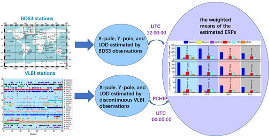
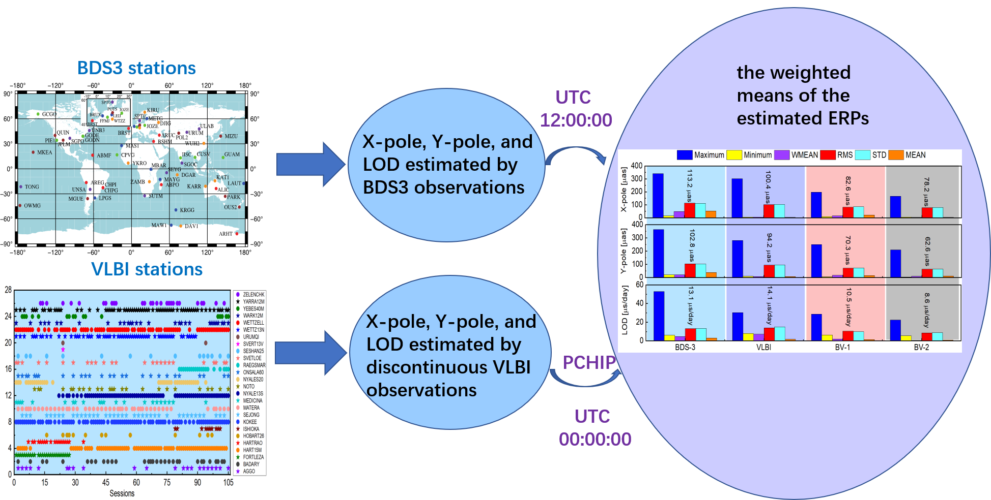
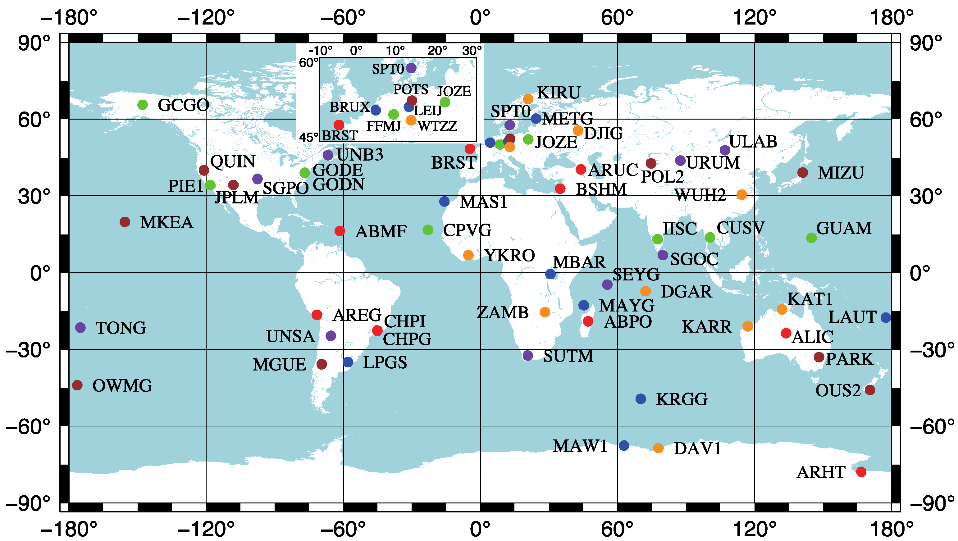
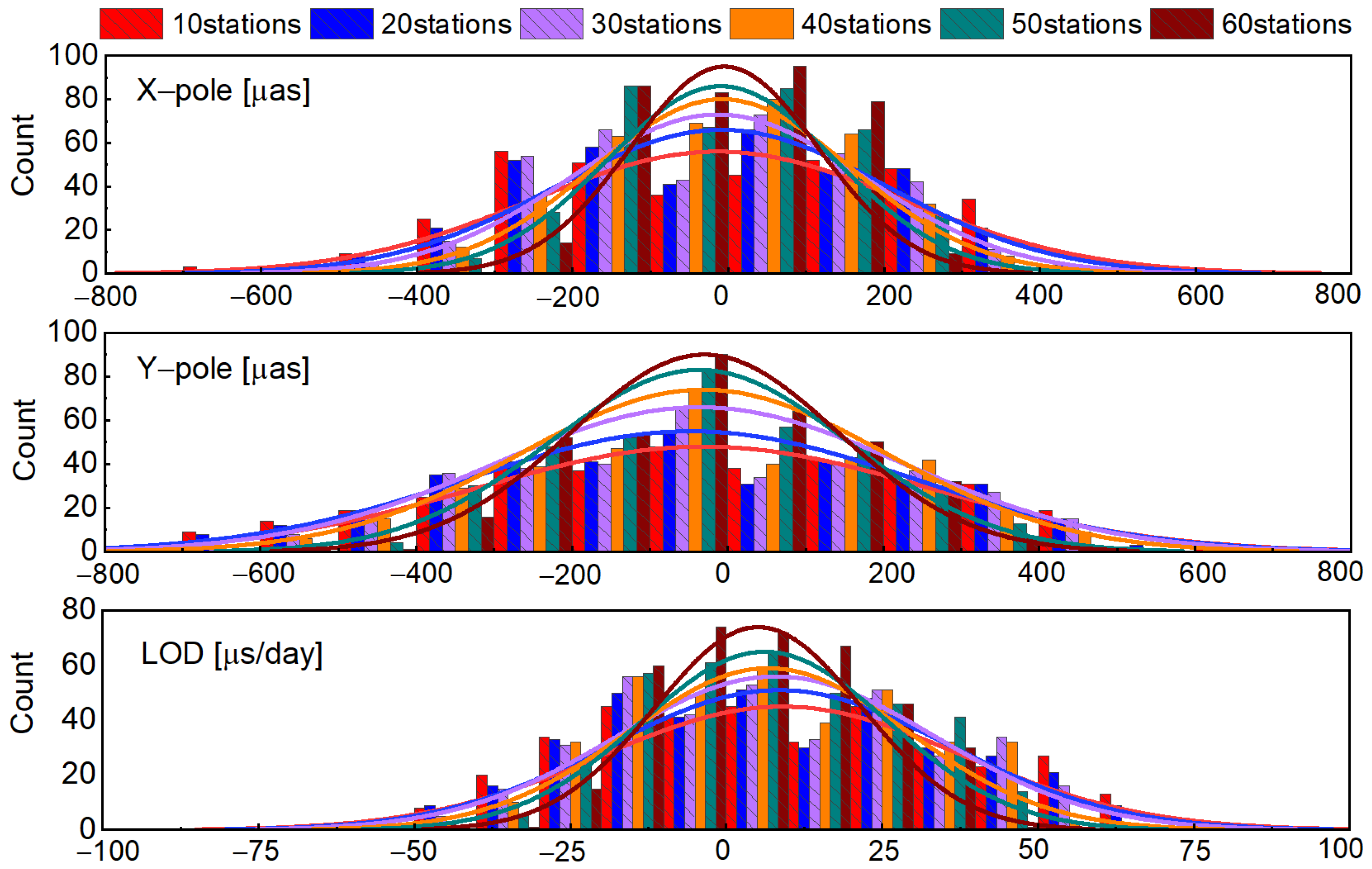
2.1. Estimating ERPs from BDS-3 Observations

Given tracking data of BDS-3 satellites from a network of ground stations, the ERPs and other parameters (such as the orbit elements of a BDS-3 satellite at an initial epoch and station coordinates) can be estimated in an orbit determination (OD) process for the BDS-3 satellites. Fundamental equations and estimation methods can be found in [30,31,32], and detailed data processing strategies are presented in

Table 1. BDS3 processing strategies.

Items	Strategy
Basic observables	BDS-3: B1I and B3I
Observation weight	Elevation (E)-dependent with a cutoff of 7 degrees. The weight is 1 if E > 30 deg, otherwise 2 $\times$ sin(E)
N-body gravitation	Jet Propulsion Laboratory (JPL) DE405 [40]
Estimator	LSQ in batch mode
Geopotential	12 × 12 EGM2008 model [41]
Sampling rate and arc length	300 s sampling, 1 day OD arc length
Attitude mode	Yaw-steering model for BDS3 [42]
Solar radiation	The 5-parameter ECOM model [43]
Satellite antenna PCO/PCV	PCO values according to CSNO/TARC (https://www.csno-tarc.cn, accessed on 3 January 2023); ignoring PCVs
A priori reference frame	IGS20 (https://lists.igs.org/pipermail/igsmail/2022/008234.html, accessed on 3 January 2023)
Receiver antenna PCO/PCV	igs20.atx corrected for BDS3
Solid earth ties, Pole ties	IERS conventions 2010 [44]
Ocean tides	FES2004 [45] for ocean tides
Tropospheric delay	Zenith troposphere delay and gradient parameters are estimated as piecewise constant with 2-h and 24-h intervals, respectively.
Earth Rotation Parameters	Precession and Nutation: IAU2006A [46]; A priori ERPs: Bulletin A (https://garner.ucsd.edu/pub/gamit/tables/finals.data, accessed on 3 January 2023). A priori-constraints: polar motion (3 as); polar motion rates (0.3 as/day); UT1-UTC (20 µs); ΔLOD (20 ms/day).

. The cutoff satellite elevation was set to 7 degrees, and the weights of observations were determined depending on elevation. The BDS-3 data over 365 days from 18 August 2020 to 17 August 2021 was processed with the Positioning And Navigation Data Analyst software (PANDA) version 1.0 [21,38,39] which was used to estimate ERPs and other parameters from BDS-3 observations, in which each OD run was set for an orbit arc of 24 h, resulting in 365 runs. In this processing, the Phase Center Offset (PCO) values provided by the Operational Control Center (OCC) were used for the BDS3 satellites, while Phase Center Variation (PCV) values were ignored. Here, the yaw-steering mode was used for the BDS-3. ECOM5 model without initial values was applied in computing the SRP acceleration. Other information about observational models, dynamical models, and estimated parameters can be found in Table 1.

2.2. Estimating ERPs from VLBI Observations

Based on the basic observation function and theories of estimating ERPs using VLBI observation data [12,47,48,49], ERP estimation experiments were conducted. The geodetic VLBI data is stored in the vgosDb format [50], where a single vgosDb database record corresponds to a collection of observations spanning 24 h. We utilized the analysis-ready version of the database, which already resolves group delay ambiguities, estimates ionosphere delays, and detects potential clock breaks. The VLBI observations in the same period as the BDS-3 observations were processed to estimate the ERPs by the Vienna VLBI Software version 3.2 (VieVS3.2). The VLBI observation data used in this experiment come from two regular observation plans for Earth rotation monitoring, the IVS-R1 and IVS-R4 plans, which make observations usually on Monday and Thursday. The R1 and R4 are generally conducted alternately, so the number of R1 and R4 observation files obtained each year is similar, except for missing files in individual years. In our experiment, there are 53 R1 and 52 R4 files. It should be noted that VLBI data was processed in the manner of the session, with each session covering a time span of 24 h starting at 17:00–18:30. In total, only 105 sessions in the 365 days were available due to data discontinuity.

The study used discontinuous VLBI data from 26 stations for a duration of one year. To process the data, the Vienna VLBI Software 3.2 (VieVS3.2) [51], developed by the Institute of Geodesy and Geophysics in Vienna, was used, and the data processing strategies are given in Table 2. In fact, no single session had observations from all stations. Usually, a session only had observations from approximately 10 stations. In the experiment, the Gauss-Markov least squares method was used to estimate all parameters simultaneously [52]. A weighting scheme was applied during data processing to account for variations in observation quality caused by different elevation angles of radio sources. At the same time, the positions of radio sources, station positions, and all ERPs were estimated.

In the solution, we imposed a constraint of 1.3 cm on the relative variation of the piecewise linear clock, while for the zenith wet delay, this constraint was set at 1.5 cm, and the estimation interval of the respective parameters was set to 60 min [53]. It should be noted that our choice of constraints will have an impact on the results obtained. For instance, if overly strict constraints are applied to troposphere parameters, it may lead to excessively smooth estimations and result in a strong dependence of residual troposphere delays on other constraints, potentially affecting other parameters as well. Since geodetic VLBI is solely based on geometric principles, there is no direct physical relationship with the center of mass of the Earth. Instead, VLBI network stations form a polyhedron in space that is connected to the terrestrial reference frame through datum definition. To eliminate the datum defect, minimization of the translations and rotations was performed on the whole of the network, utilizing least squares [54].

Table 2. VLBI processing strategies.

Items	Strategy
Method	Gauss-Markov least squares estimation
Weighting scheme	The stand approach (SA) [55] for EOP estimation
Clock offset	Estimated as piecewise linear offsets (60 min), one rate, and one quadratic term per clock
Troposphere	Corrected by the Saastamoinen model [56] and VMF3 mapping function [57], the zenith wet delay estimation interval is 60 min and the gradient parameters were not estimated
Ionosphere	Ionospheric free combination
ERPs	Bulletin A is used as a priori model, and the resolution for the estimated ERPs is 24 h.
Source coordinate	Estimated
Station coordinate	Estimated as one offset each session
ITRF/ICRF model	ITRF2020 [58], ICRF3 [59]
Solid Earth tides, pole tides	IERS Conventions 2010
Ocean tides	FES2004 [45]
Earth Rotation Parameters	The X-pole, Y-pole, UT1-UTC are estimated, and their constraints: polar motion (2 mas); UT1-UTC (20 µs)
Other parameters	Using the default values provided by VieVS software version 3.2 (VieVS3.2)

Table 2. VLBI processing strategies.

Items	Strategy
Method	Gauss-Markov least squares estimation
Weighting scheme	The stand approach (SA) [55] for EOP estimation
Clock offset	Estimated as piecewise linear offsets (60 min), one rate, and one quadratic term per clock
Troposphere	Corrected by the Saastamoinen model [56] and VMF3 mapping function [57], the zenith wet delay estimation interval is 60 min and the gradient parameters were not estimated
Ionosphere	Ionospheric free combination
ERPs	Bulletin A is used as a priori model, and the resolution for the estimated ERPs is 24 h.
Source coordinate	Estimated
Station coordinate	Estimated as one offset each session
ITRF/ICRF model	ITRF2020 [58], ICRF3 [59]
Solid Earth tides, pole tides	IERS Conventions 2010
Ocean tides	FES2004 [45]
Earth Rotation Parameters	The X-pole, Y-pole, UT1-UTC are estimated, and their constraints: polar motion (2 mas); UT1-UTC (20 µs)
Other parameters	Using the default values provided by VieVS software version 3.2 (VieVS3.2)

3. Results

In the result assessment, the EOP 20C04 series released by the IERS (https://www.iers.org, accessed on 5 January 2023), which is the combined result of VLBI, SLR, GNSS, and DORIS solutions, was used as the reference. The IERS uses a set of algorithms to analyze and synthesize these data and generates a relatively smooth and more accurate product. In this paper, we used the IERS EOP 20C04 as the reference, which officially replaced the EOP 14C04 series since 14 February 2023.

In this study, the accuracy of the ERPs estimated by BDS-3, VLBI, and the combination of the BDS-3 and VLBI solutions was analyzed for multiple sets of experiments. The experimental schemes were as follows:

Scheme 1: ERPs estimated based on the BDS-3 observations (the effects of satellite type, number of stations, and polyhedron volume of stations on the accuracy of estimating ERPs are discussed, respectively);

Scheme 2: ERPs estimated based on the VLBI observations (the effect of the polyhedron volume of stations on the accuracy of estimating ERPs is discussed);

Scheme 3: ERPs estimated based on combining BDS-3 and VLBI solutions.

3.1. Daily ERP Series Estimated Using BDS-3 Observations

To assess the accuracy and stability of the daily ERPs series estimated using BDS-3 data, a comprehensive analysis was conducted utilizing data from 60 stations within the International GNSS Service (IGS). The geographical distribution of these stations is depicted in Figure 1, and the stations in the first to sixth groups are represented by red, green, blue, brown, purple, and orange dots, respectively. The names of the stations used in the experiment are shown in

Table 3. The names of the stations used in the experiment.

Group	Stations
Group 1	ABMF	ABPO	ALIC	AREG	ARHT	ARUC	BRST	BSHM	CHPG	CHPI
Group 2	CPVG	CUSV	FFMJ	GCGO	GODE	GODN	GUAM	IISC	JOZE	JPLM	plus Group 1
Group 3	KRGG	LAUT	LEIJ	BRUX	LPGS	MAS1	MAW1	MAYG	MBAR	METG	plus Group 2
Group 4	MGUM	MIZU	MKEA	OUS2	OWMG	PARK	PIE1	POL2	POTS	QUIN	plus Group 3
Group 5	SEYG	SGOC	SGPO	SPT0	SUTM	TONG	ULAB	UNB3	UNSA	URUM	plus Group 4
Group 6	WTZZ	DGAR	WUH2	YKRO	ZAMB	DJIG	DAV1	KIRU	KAT1	KARR	plus Group 5

. The IGS launched the Multi-GNSS Experiment (MGEX) project in 2012 with the aim of collecting and analyzing data on emerging new signals and systems [60]. As part of this initiative, starting in 2013, the MGEX network began providing observation data for BDS [61], and BDS-3 B1I/B3I data has been available since 2019. For this study, BDS-3 observations from 18 August 2020 to 17 August 2021 were selected. The ERPs estimated from the BDS-3 observations were compared to the IERS EOP 20C04.

To investigate the impact of the number of stations on the accuracy of estimated ERPs, we conducted experiments using six groups of BDS-3 stations, as listed in Table 3. The 6 groups have 10, 20, 30, 40, 50, and 60 stations, respectively, where the new group consists of the last group and 10 new stations; for example, Group 2 consists of stations in Group 1 and 10 more new stations, and Group 3 consists of stations in Group 2 and 10 more new stations. Figure 2 depicts the distributions of disparities among all groups between the estimated ERPs and IERS 20 C04 time series. It is evident that these disparities demonstrate a strong correlation with the number of stations utilized. As the number of stations increased, the range of disparities became smaller and smaller. When the number of stations increased from 10 to 40, most of the X-pole and Y-pole differences decreased from $\pm 600\mathrm{\mu }\mathrm{a}\mathrm{s}$ to $\pm 400\mathrm{\mu }\mathrm{a}\mathrm{s}$ and most of the LOD differences decreased from $\pm 70\mathrm{\mu }\mathrm{s}/\mathrm{d}\mathrm{a}\mathrm{y}$ to $\pm 50\mathrm{\mu }\mathrm{s}/\mathrm{d}\mathrm{a}\mathrm{y}$. When the number of stations was 60, most of the X-pole and Y-pole differences were within $\pm 300\mathrm{\mu }\mathrm{a}\mathrm{s}$ and most of the LOD differences were within $\pm 30\mathrm{\mu }\mathrm{s}/\mathrm{d}\mathrm{a}\mathrm{y}$.

Table 4. The RMS and STD values of ERP differences between BDS-3 solutions and the IERS EOP 20C04 products.

Statistics Stations	X-Pole [µas]			Y-Pole [µas]			LOD [µs]
	RMS	STD	MEAN	RMS	STD	MEAN	RMS	STD	MEAN
10	170.2	170.1	−13.0	160.1	161.5	−21.3	18.3	18.4	8.9
20	161.0	160.4	−8.4	148.3	150.2	−29.5	17.2	17.3	8.5
30	143.3	145.3	−13.5	135.6	136.7	−22.6	16.2	16.1	7.9
40	130.2	130.6	−7.6	120.4	120.5	−17.4	14.8	14.9	6.8
50	122.3	122.4	−8.9	117.5	113.5	−18.7	14.1	14.1	6.2
60	113.2	110.1	−4.9	102.8	102.3	−16.8	13.1	13.3	5.1

presents the root mean square (RMS), standard deviation (STD), and average values of the differences in X-pole, Y-pole, and LOD. Utilizing a total of 10 stations, the RMS values for X-pole and Y-pole were found to be 170.2 µas and 160.1 µas, while that for LOD was 18.3 µs/day. The RMS values for the polar motion components gradually decreased when the number of stations increased, and the RMS for LOD became stable when the number of stations was more than 40. Using all 60 stations, the RMS of the differences was 113.2 µas for X-pole, 102.8 µas for Y-pole, and 13.1 µs for LOD.

The effect of the number of stations on the estimation accuracy of ERPs can be further analyzed by examining the volume of polyhedrons formed by these stations. As shown in Figure 3, it is observed that, as the number of stations increased, the volume of the polyhedron grew. Interestingly, comparing two variations of station numbers, namely the variation from 10 to 40 and that from 40 to 60, it is found that there was a larger volume change in the first variation compared to the second. This observation aligns with the statistical data presented in Table 4 regarding ERPs estimated using BDS-3. To gain a visual understanding of how different station networks contribute to this phenomenon, Figure 4 illustrates the polyhedral shapes formed by the stations in the 6 groups. Through conducting these experiments and analyzing their results, we can infer that both the number of stations and network geometry volume play significant roles in determining ERP estimation accuracy. Specifically, having a larger network with more stations and larger polyhedral volumes tends to lead to more accurate ERP estimation. To assess the effect of the polyhedral volume on the ERP estimation accuracy, each volume of the six polyhedrons was computed in the following way:

1. The tetrahedron mesh for a polyhedron was computed through Delaunay triangulation utilizing the GEOMPACK package [62].

2. The volume calculation for each tetrahedron involved evaluating its scalar triple product according to Equation (1):

$$\left|\left({\mathit{r}}_2-{\mathit{r}}_1\right)·\left({\mathit{r}}_3-{\mathit{r}}_1\right)\times \left({\mathit{r}}_4-{\mathit{r}}_1\right)\right|/6$$

(1)

where ${\mathit{r}}_1,{\mathit{r}}_2,{\mathit{r}}_3,{\mathit{r}}_4$ represent geocentric station position vectors.

3. Compute the total network volume as the sum of the volumes of all the tetrahedrons.

In summary, our findings suggest that considering both the number of stations and network geometry is crucial when aiming for highly accurate ERP estimation using BDS-3 data.

Considering that the BDS-3 has MEO, IGSO, and GEO satellites, it is interesting to see the contributions of different satellites to the ERP estimation. Three cases were experimented with. In the first case, all MEO, IGSO, and GEO satellites were used. The second case had both MEO and IGSO satellites, and the third case only had MEO satellites. We analyzed the results from 60 stations, and the distributions of the differences between the estimated and reference EOP 20C04 ERPs, as well as the mean and STD of the differences, are shown in Figure 5.

It is seen that using the MEO satellites only generated the best results; the second-best results were from the use of the MEO and IGSO satellites together, while the use of all satellites delivered the worst results in terms of RMSs. From the left panel in Figure 5, it is seen that most of the differences in X-pole were within ±400 µas when only the MEO satellites were used. When the IGSO satellites were included, the absolute maximum value of the differences in X-pole was 473 µas; it was 510 µas when both the IGSO and GEO satellites were included. The STD values in the X-pole were 128.4 µas, 120.6 µas, and 110.1 µas for the three cases, respectively. In the middle panel in Figure 5, the differences in Y-pole were within ±500 µas, but those with MEO satellites only were mostly within ±300 µas. Using both the MEO and IGSO satellites resulted in a Y-pole STD of 117.1 µas, larger than that using only the MEO satellites. The Y-pole STD using all satellites was the largest. From the bottom panel in Figure 5, most of the differences in LOD were within ±300 µs/day. The STD value of LOD differences from the use of MEO satellites only was 13.3 µs; it was 16.8 µs/day when the IGSO satellites were included, and it increased to 20.1 µs when all satellites were used. According to these experiments, the inclusion of the IGSO and GEO satellites of BDS-3 in the estimation of the ERPs does not improve the accuracy. Further studies are needed to find the reasons.

3.2. Analysis of Daily ERP Series Estimated by VLBI Observations

The distribution of VLBI stations involved in this experiment was predominantly concentrated in the Northern Hemisphere, as shown in Figure 6 and Figure 7, which illustrate the stations used in each of the 105 sessions. Due to the intermittent nature of VLBI observation data, it is necessary to estimate ERPs for days without VLBI data using interpolation techniques. In this study, we utilized the Piecewise Cubic Hermite Interpolation Polynomial (PCHIP) method [63] for the ERP interpolation. It is noted that other interpolation methods, namely the linear, Akima, spline, Newton, and Lagrange methods, were used to obtain the ERPs on days without VLBI data. It was found that applying the PCHIP method resulted in the smallest differences between the interpolated and reference IERS EOP 20C04 ERPs.

Figure 8 depicts the differences between the ERPs estimated by the VLBI and EOP 20C04 series, as well as the mean and STD values. The differences in X-pole and Y-pole were within ±500 µas, whereas for LOD they were within ±50 µs/day. The STD values of the X-pole, Y-pole, and LOD were 103.1 µas, 96.5 µas, and 15.2 µs/day, respectively. The volumes of VLBI-station polyhedrons and the number of stations for all 105 sessions are shown in Figure 9. It can be seen that the number of stations was not necessarily proportional to the volume. For example, the number of stations in session 1 was greater than that in session 9, but the volume of session 1 was smaller than that of session 9 because the volume is strongly dependent on the geometrical distribution of the stations. However, a session with a large polyhedron volume will generate a more accurate estimate of the ERPs. This is clearly shown in Figure 10, which shows that the volume was inversely proportional to the accuracy of the X-pole and Y-pole, and this was also generally true for LOD. One can see that, even with the same number of stations, such as in sessions 7 and 9, the volume with respect to session 7 was larger than that with session 9, and the accuracy in session 9 was higher than that in session 7.

The relationship between the ERP estimation accuracy and the polyhedral volume of the VLBI network can also be studied using the method proposed by Malkin [64]. That is, the precision of an ERP parameter, $\sigma$, can be modeled as a power function of the polyhedral volume, $a{V}^y$, where $V$ is the volume with respect to a VLBI network, $a$ and $y$ are the model coefficients. In this experiment, we only compared the precision of the X-pole and Y-pole with the results of Malkin’s. Applying the Malkin model and the coefficients for the precision model, the model precisions of all the 105 VLBI sessions were obtained and shown in Figure 11. It is noted that the 105 VLBI sessions are arranged from small to large in the order of the polyhedral volume on the x-axis. From the figure, it is seen that, for most of the 105 sessions, the model precision agreed well with the VLBI precision in this paper. Using the average volumes of these 105 sessions, one obtained the model precisions for X-pole and Y-pole, respectively. The averages of the corresponding VLBI precisions in this paper agreed very well with the respective model precisions in each group.

3.3. Analysis of the Daily ERP Series from the Combination of VLBI and BDS-3

The combination of the VLBI and BDS3 techniques for estimating ERPs has two significant advantages. First, the combination is helpful to make up for the shortcomings because of the discontinuous observation data and the few observation stations in the case of the VLBI technology. Second, in terms of result stability, the combination is much better than using only the BDS-3 or VLBI technology.

The combination of the estimated ERPs was performed using the following two methods: the weighted averaging method, Equation (2) below; and the normal equation combination method [65]. In Equation (2), $\sigma$ is the standard deviation of the least-squares estimated parameter. On days without VLBI observations, the PCHIP method is used to obtain the VLBI ERPs and their standard deviations.

$${ERP}_{-}BV1=\frac{{\sigma }_{VLBI}^2\cdot {ERP}_{BDS}+{\sigma }_{BDS}^2\cdot {ERP}_{VLBI}}{{\sigma }_{VLBI}^2+{\sigma }_{BDS}^2}$$

(2)

Below, we compare the accuracy of different ERPs. The following 6 cases are considered:

Case 1: 105 BDS-3 solutions corresponding to the VLBI sessions, named as BDS-3-105;

Case 2: 105 VLBI observation-day solutions, named VLBI-105;

Case 3: VLBI solutions over the time from 18 August 2020 to 17 August 2021, where the interpolated results were used on days without VLBI observations, named VLBI-105-PCHIP;

Case 4: BDS-3 solutions over the time from 18 August 2020 to 17 August 2021, named BDS-3-all;

Case 5: Weighted averaging solutions of Case 3 and Case 4, named BV-1;

Case 6: Normal equation combination solutions of Case 3 and Case 4, named BV-2.

Currently, due to the discontinuity of VLBI observation data, we need to use an interpolation method to obtain the ERPs on days without VLBI data. In Case 1 and Case 2, 105-day ERPs were estimated from BDS-3 observations on days having VLBI data and VLBI observations, respectively, and there was no interpolation needed. In Case 3, the VLBI-105-PCHIP was the result containing both the 105-day ERPs from processing the VLBI data and the interpolated ERPs on days without VLBI data using the PCHIP method. The BDS-3-all results in Case 4 were estimated from BDS-3 observations for 365 days. Therefore, the results in Case 1 and Case 2 were for the 105 days having VLBI data, and the results in Case 3 and Case 4 were for 365 days. The BV-1 results in Case 5 were obtained using the weighted average method with the inputs from the results in Case 3 and Case 4. The BV-2 results in Case 6 were obtained using the normal equation combination, in which the station coordinates, ERP parameters, prior coordinates, covariance, prior covariance, etc. provided by the SINEX file of BDS and VLBI solutions were used to form the normal equations. The joint processing of multiple spatial geodetic techniques was achieved by adding Helmert parameters and stacking the normal equations to solve the combined ERP parameters. It is noted that the PCHIP method was adopted because it performed better than other interpolation methods.

From the statistical results in Figure 12, it can be seen that, for the X-pole and Y-pole, VLBI-105 had smaller RMS values than BDS-3-105, indicating that VLBI is better in the PM estimation. This is also the case even when the interpolated ERPs on days without VLBI data were included in the comparison. For the LOD, it was the BDS-3 that had a smaller RMS. It is clear that the RMS values of ERPs through the weighted averaging or the normal equation combination were all smaller than their counterparts with a single technique, with the normal equation combination outperforming the weighted averaging. Comparing the RMS values of BV-2 with those in the first 5 cases, we obtained the estimation accuracy improvement, listed in

Table 5. RMS reduction using the normal equation combination method.

ERPs	BDS-3-105	VLBI-105	VLBI-105-PCHP	BDS-3-all	BV-1
X-pole	35.4%	24.4%	22.1%	30.9%	5.3%
Y-pole	44.3%	36.3%	33.5%	39.1%	11.0%
LOD	31.7%	41.9%	39.0%	34.4%	18.1%

, with the BV-2 RMS as the base.

The differences between the reference and the ERPs in Cases 3 to 6 are shown in Figure 13, where the means and STD of the differences are also given. The results show that approximately 38.6%, 42.4%, 63.5%, and 79.2% of differences for X-pole were within ±100 µas, respectively, for BDS-3, VLBI, BV-1, and BV-2 solutions. For Y-pole, 34.1%, 60.3% 71.2%, and 85.8% of the differences were within ±100 µas. For LOD, 62.1%, 58.0% 77.4%, and 86.2% of the differences were within ±20 µs. With the standard deviation, the BV-2 solution had the smallest STD, followed by BV-1, and BDS-3 had the largest STD value for PM. It is also noted that the means of differences in BV-2 solutions were significantly smaller than those of other solutions.

Overall, the accuracy of the combined ERPs, whether through the weighted averaging or the normal equation combination, was better than that obtained from the use of BDS-3 alone or VLBI alone. This demonstrates that the combination of different technologies can effectively improve the accuracy of ERPs estimation.

Figure 14 shows the maximum, minimum, WMEAN, RMS, STD, and mean values of the differences for the solutions from the BDS-3 alone, VLBI alone, weighted averaging, and normal equation combination. For the BDS-3 solution, the RMS values were 113.2 µas, 102.8 µas, and 13.1 µs/day for X-pole, Y-pole, and LOD, respectively. Comparatively, for the VLBI solution, we observe slightly lower RMS values with 100.4 µas for X-pole, 94.2 µas for Y-pole but higher 14.1 µs for LOD. On the other hand, the accuracy of the BV-1 solution was better than that of the BDS-3 solution, and also more stable. The RMS values for X-pole, Y-pole, and LOD of the BV-1 solution were 82.6 µas, 70.3 µas, and 10.5 µs/day, respectively. The RMS values of the BV-2 solutions were 78.2 µas, 62.6 µas, and 8.6 µs/day for X-pole, Y-pole and LOD, respectively. These findings suggest that combining ERP results (BV-1 and BV-2) from BDS-3 and VLBI leads to more accurate results than the results from only BDS-3 or VLBI data.

4. Discussion

This study is dedicated to exploring the accuracy of the ERPs estimated by BDS-3 and discontinuous VLBI observations. The experiments were mainly performed as ERP estimation based on BDS-3 alone, VLBI alone, and a combination of BDS-3 and VLBI solutions.

On estimating ERP based on BDS-3 technology, two experiments with one focusing on the number of stations and the other on satellite types were conducted. Six groups with the number of stations in 10, 20, 30, 40, 50, and 60, respectively, were formed to see the effects of the number of stations, in particular, the volume of the polyhedron formed by the stations, on the ERP estimation accuracy. The accuracy was higher when more stations were used, and when using all 60 stations was the highest. It was seen that when the number of stations increased from 40 to 60, the accuracy improvement was less significant, but the calculation time increased significantly. It was also seen that, the larger the volume of polyhedron formed by the stations, the higher the accuracy of ERP. However, the ERP estimation accuracy using BDS-3 appeared less accurate than that using GPS, most likely due to lower BDS-3 observation accuracy. Experiments on the use of satellites in different sub-constellations showed that the ERP accuracy estimated based on IGSO + MEO satellites or MEO satellites alone was better than that using GEO + IGSO + MEO satellites, and using MEO satellites only produced the best results. In theory, including IGSO/GEO data should not produce less accurate ERP estimates, if appropriate weights between IGSO/GEO data and MEO data are applied. We will investigate the appropriate weight schemes in the future.

Experiment results of estimating ERP based on VLBI technology were analyzed on the relation between the volume of polyhedra formed by VLBI stations and ERP estimation accuracy, and also compared with those using the model of Malkin (replacing the results in Table 4 with WRMS for consistency with Malkin), verifying the model’s appropriateness. It is noted that, although the UT1-UTC was estimated, the presented results were the LODs converted from the UT1-UTC for the sake of comparison and combination with BDS-3 LODs.

In obtaining the combined ERPs from the BDS-3 and VLBI solutions, we used the weighted average method, resulting in the combination solution BV-1, and the normal equation combination method, resulting in BV-2. It was shown that both combination results were better than the ERP results estimated by a single technique, and BV-2 was superior to BV-1.

Overall, the combination of continuous BDS-3 observations and discontinuous VLBI observations can effectively improve the accuracy of ERP estimation, and the combination of multiple space technologies will bring more opportunities for ERP estimation.

5. Conclusions

Leveraging the abundant resources provided by a global network of ground tracking stations and the continuous observational data, the GNSS has established itself as an indispensable technology for the precise estimation of Earth Rotation Parameters (ERPs). With its full operation, the BDS-3 becomes another source for the estimation of the ERPs. This study presents the results of estimating ERPs by the use of BDS-3 data over 365 days from as many as 60 stations, as well as those from the VLBI data of 26 stations in the same time period. The estimated ERPs were compared with those in the IERS EOP 20C04 in the accuracy assessment.

Applying the weighted averaging method, the RMS values of the solution decreased by 27.0%, 31.6%, and 19.8% for X-pole, Y-pole, and LOD, respectively, compared to those of the BDS-3 solution. The reductions were 17.7%, 25.4%, and 25.5% against those of the VLBI solution. The decreases were bigger when the normal equation combination method was used to fuse the VLBI and BDS-3 solutions. The corresponding reductions were 30.9%, 39.5%, and 34.4% compared to those of the BDS-3 solution, and were 22.1%, 33.5%, and 39.0% with respect to those of the VLBI solution. Overall, the combination of BDS-3 and VLBI solutions can effectively improve the accuracy of ERP estimation, with the normal equation combination outperforming the weighted averaging.

This paper also investigated the relationship between ERP estimate accuracy the number of tracking stations used, and the volume of polyhedron formed by the stations. The experiment of estimating ERP using BDS-3 and VLBI single technology shows that when the number of stations used was the same, the larger the polyhedral volume formed by the stations, the higher the accuracy of ERP estimation. When the polyhedral volume was the same, the number of stations may not be the same, but the accuracy of ERP estimation was close.

It is believed that, if BDS-3 is replaced with other GNSS, such as GPS, the combined ERP results using the weighted average and normal equation combination methods would have an improvement in accuracy than that of single technology solution. Moreover, our work is planned for implementing the combination at the observation level and multi-GNSS data from BDS-3, GPS, GALILEO, and GLONASS may be better fused in the ERP estimation at the observation level.

References

1. Gambis, D. Monitoring Earth orientation using space-geodetic techniques: State-of-the-art and prospective. J. Geod. 2004, 78, 295–303. [Google Scholar] [CrossRef]
2. Kalarus, M.; Schuh, H.; Kosek, W.; Akyilmaz, O.; Bizouard, C.; Gambis, D.; Gross, R.; Jovanović, B.; Kumakshev, S.; Kutterer, H.; et al. Achievements of the Earth orientation parameters prediction comparison campaign. J. Geod. 2010, 84, 587–596. [Google Scholar] [CrossRef]
3. Kouba, J. Sub-daily earth rotation parameters and the international Gps service orbit clock solution products. Stud. Geophys. Geod. 2002, 46, 9–25. [Google Scholar] [CrossRef]
4. Lutz, S.; Beutler, G.; Schaer, S.; Dach, R.; Jäggi, A. CODE’s new ultra-rapid orbit and ERP products for the IGS. GPS Solut. 2016, 20, 239–250. [Google Scholar] [CrossRef]
5. Bizouard, C.; Lambert, S.; Gattano, C.; Becker, O.; Richard, J.Y. The IERS EOP 14C04 solution for Earth orientation parameters consistent with ITRF 2014. J. Geod. 2019, 93, 621–633. [Google Scholar] [CrossRef]
6. Seitz, M.; Angermann, D.; Bloßfeld, M.; Drewes, H.; Gerstl, M. The 2008 DGFI realization of the ITRS: DTRF2008. J. Geod. 2012, 86, 1097–1123. [Google Scholar] [CrossRef]
7. Kern, M.; Schwarz, K.P.; Sneeuw, N. A study on the combination of satellite, airborne, and terrestrial gravity data. J. Geod. 2003, 77, 217–225. [Google Scholar] [CrossRef]
8. Dettmering, D.; Schmidt, M.; Heinkelmann, R.; Seitz, M. Combination of different space-geodetic observations for regional ionosphere modeling. J. Geod. 2011, 85, 989–998. [Google Scholar] [CrossRef]
9. Krügel, M.; Thaller, D.; Tesmer, V.; Rothacher, M.; Angermann, D.; Schmid, R. Tropospheric parameters: Combination studies based on homogeneous VLBI and GPS data. J. Geod. 2007, 81, 515–527. [Google Scholar] [CrossRef]
10. Buetler, G.; Pearlman, M.; Plag, H.; Neilan, R.; Rummel, R. Global Geodetic Observing System: Meeting the Requirements of a Global Society on a Changing Planet in 2020; Springer: Berlin/Heidelberg, Germany, 2009. [Google Scholar]
11. Nilsson, T.; Böhm, J.; Schuh, H.; Schreiber, U.; Gebauer, A.; Klügel, T. Combining VLBI and ring laser observations for determination of high frequency Earth rotation variation. J. Geodyn. 2012, 62, 69–73. [Google Scholar] [CrossRef]
12. Nilsson, T.; Heinkelmann, R.; Karbon, M.; Raposo-Pulido, V.; Soja, B.; Schuh, H. Earth orientation parameters estimated from VLBI during the CONT11 campaign. J. Geod. 2014, 88, 491–502. [Google Scholar] [CrossRef]
13. Hobiger, T.; Rieck, C.; Haas, R.; Koyama, Y. Combining GPS and VLBI for iner-continental frequency transfer. Metrologia 2015, 52, 251. [Google Scholar] [CrossRef]
14. Nothnagel, A.; Artz, T.; Behrend, D.; Malkin, Z. International VLBI Service for Geodesy and Astrometry: Delivering high-quality products and embarking on observations of the next generation. J. Geod. 2016, 91, 711–721. [Google Scholar] [CrossRef]
15. Nothnagel, A.; Anderson, J.; Behrend, D.; Böhm, J.; Charlot, P.; Colomer, F.; Witt, A.d.; John, G.; Haas, R.; Hall, D. IVS Infrastructure Development Plan 2030; 2021. Available online: http://hdl.handle.net/20.500.12708/40332 (accessed on 3 January 2023).
16. Dow, J.M.; Neilan, R.E.; Rizos, C. The International GNSS Service in a changing landscape of Global Navigation Satellite Systems. J. Geod. 2009, 83, 191–198. [Google Scholar] [CrossRef]
17. Ferland, R.; Piraszewski, M. The IGS-combined station coordinates, earth rotation parameters and apparent geocenter. J. Geod. 2009, 83, 385–392. [Google Scholar] [CrossRef]
18. Ray, J.; Rebischung, P.; Griffiths, J. IGS polar motion measurement accuracy. Geod. Geodyn. 2017, 8, 413–420. [Google Scholar] [CrossRef]
19. Ray, J.; Altamimi, Z. Evaluation of co-location ties relating the VLBI and GPS reference frames. J. Geod. 2005, 79, 189–195. [Google Scholar] [CrossRef]
20. Ray, J.; Kouba, J.; Altamimi, Z. Is there utility in rigorous combinations of VLBI and GPS Earth orientation parameters? J. Geod. 2005, 79, 505–511. [Google Scholar] [CrossRef]
21. Wang, J.; Ge, M.; Glaser, S.; Balidakis, K.; Heinkelmann, R.; Schuh, H. Impact of Tropospheric Ties on UT1-UTC in GNSS and VLBI Integrated Solution of Intensive Sessions. J. Geophys. Res. Solid Earth 2022, 127, e2022JB025228. [Google Scholar] [CrossRef]
22. Wang, J.; Ge, M.; Glaser, S.; Balidakis, K.; Heinkelmann, R.; Schuh, H. Improving VLBI analysis by tropospheric ties in GNSS and VLBI integrated processing. J. Geod. 2022, 96, 32. [Google Scholar] [CrossRef]
23. Thaller, D.; Krügel, M.; Rothacher, M.; Tesmer, V.; Schmid, R.; Angermann, D. Combined Earth orientation parameters based on homogeneous and continuous VLBI and GPS data. J. Geod. 2007, 81, 529–541. [Google Scholar] [CrossRef]
24. Bourda, G.; Charlot, P.; Biancale, R. VLBI analyses with the GINS software for multi-technique combination at the observation level. In Proceedings of the SF2A-2008: Annual Meeting of the French Society of Astronomy and Astrophysics, Paris, France, 30 June–4 July 2008. [Google Scholar]
25. Hobiger, T.; Otsubo, T.; Sekido, M. Observation level combination of SLR and VLBI with c5++: A case study for TIGO. Adv. Space Res. 2014, 53, 119–129. [Google Scholar] [CrossRef]
26. CSNO. BeiDou Navigation Satelite System B2a, Version 1.0; CSNO China Satellite Navigation Office: Beijing, China, 2017. [Google Scholar]
27. CSNO. BeiDou Navigation Satellite System Signal In Space Interface Control Document Open Service Signal B3I, Version 1.0; CSNO China Satellite Navigation Office: Beijing, China, 2018. [Google Scholar]
28. CSNO. Development of the BeiDou Navigaton Satelite System, Version 4.0; CSNO China Satellite Navigation Office: Beijing, China, 2019. [Google Scholar]
29. CSNO. BeiDou Navigation Satellite System Open Service Performance Standard, Version 3.0; CSNO China Satellite Navigation Office: Beijing, China, 2021. [Google Scholar]
30. Tianhe, X.; Sumei, Y.; Jianjin, L. Earth Rotation Parameters Determination Using BDS and GPS Data Based on MGEX Network. In China Satellite Navigation Conference (CSNC) 2014 Proceddings; Springer: Berlin/Heidelberg, Germany, 2014; pp. 289–299. [Google Scholar]
31. Li, M.; Xu, T. Research on the Combination of IGS Analysis-Center Solution for station Coordinates and ERPs. In Proceedings of the China Satellite Navigation Conference (CSNC), Nanjing, China, 21–23 May 2014; pp. 15–30. [Google Scholar]
32. Fang, X.; Fan, L.; Guo, S.; Zhou, L.; Shi, C. Earth Rotation Parameters Determination with BDS-3/LEO Simulations under Small-Scale Ground Networks. In Proceedings of the China Satellite Navigation Conference (CSNC 2022) Proceedings; Springer: Singapore, 2022; Volume III, pp. 102–112. [Google Scholar]
33. Johnston, G.; Riddell, A.; Hausler, G. The international GNSS service. In Springer Handbook of Global Navigation Satellite Systems; Springer: Berlin/Heidelberg, Germany, 2017; pp. 967–982. [Google Scholar] [CrossRef]
34. Duan, B.; Hugentobler, U.; Selmke, I.; Marz, S.; Killian, M.; Rott, M. BeiDou Satellite Radiation Force Models for Precise Orbit Determination and Geodetic Applications. IEEE Trans. Aerosp. Electron. Syst. 2022, 58, 2823–2836. [Google Scholar] [CrossRef]
35. Zajdel, R.; Sośnica, K.; Bury, G.; Dach, R.; Prange, L. System-specific systematic errors in earth rotation parameters derived from GPS, GLONASS, and Galileo. GPS Solut. 2020, 24, 74. [Google Scholar] [CrossRef]
36. Peng, Y.; Lou, Y.; Dai, X.; Guo, J.; Shi, C. Impact of solar radiation pressure models on earth rotation parameters derived from BDS. GPS Solut. 2022, 26, 126. [Google Scholar] [CrossRef]
37. He, Z.; Wei, E.; Zhang, Q.; Wang, L.; Li, Y.; Liu, J. Earth rotation parameters from BDS, GPS, and Galileo data: An accuracy analysis. Adv. Space Res. 2023, 71, 3968–3980. [Google Scholar] [CrossRef]
38. Liu, J.; Ge, M. PANDA Software and its Preliminary Result of Positioning and Orbit Determination. Wuhan Univ. J. Nat. Sci. 2003, 8, 603–609. [Google Scholar] [CrossRef]
39. Liu, Y.; Ge, M.; Shi, C.; Lou, Y.; Wickert, J.; Schuh, H. Improving integer ambiguity resolution for GLONASS precise orbit determination. J. Geod. 2016, 90, 715–726. [Google Scholar] [CrossRef]
40. Standish, E.M. JPL Planetary and Lunar Ephemerides, DE405/LE405. JPL IOM 1998, 312, F-98-048. [Google Scholar]
41. Pavlis, N.K.; Holmes, S.A.; Kenyon, S.C.; Factor, J.K. The development and evaluation of the Earth Gravitational Model 2008 (EGM2008). J. Geophys. Res. Solid Earth 2012, 117, B4. [Google Scholar] [CrossRef]
42. Wang, C.; Guo, J.; Zhao, Q.; Liu, J. Yaw attitude modeling for BeiDou I06 and BeiDou-3 satellites. GPS Solut. 2018, 22, 117. [Google Scholar] [CrossRef]
43. Arnold, D.; Meindl, M.; Beutler, G.; Dach, R.; Schaer, S.; Lutz, S.; Prange, L.; Sośnica, K.; Mervart, L.; Jäggi, A. CODE’s new solar radiation pressure model for GNSS orbit determination. J. Geod. 2015, 89, 775–791. [Google Scholar] [CrossRef]
44. Petit, G.; Luzum, B. IERS Conventions (2010); IERS Technical Note 36; Verlag des Bundesamts für Kartographie und Geodäsie: Frankfurt am Main, Germany, 2010. [Google Scholar]
45. Lyard, F.; Lefevre, F.; Letellier, T.; Francis, O. Modelling the global ocean tides: Modern insights from FES2004. Ocean Dyn. 2006, 56, 394–415. [Google Scholar] [CrossRef]
46. Vincent, C.; Seago, J.H.; Vallado, D.A. The IAU 2000A and IAU 2006 precession-nutation theories and their implementation. Adv. Astronaut. Sci. 2009, 919–938. Available online: https://www.researchgate.net/publication/289753602 (accessed on 10 January 2023).
47. Böhm, J.; Böhm, S.; Nilsson, T.; Pany, A.; Plank, L.; Spicakova, H.; Teke, K.; Schuh, H. The New Vienna VLBI Software VieVS. In Geodesy for Planet Earth: Proceedings of the 2009 IAG Symposium, Buenos Aires, Argentina, 31 August–4 September 2009; Springer: Berlin/Heidelberg, Germany, 2012; pp. 1007–1011. [Google Scholar]
48. Schuh, H.; Behrend, D. VLBI: A fascinating technique for geodesy and astrometry. J. Geodyn. 2012, 61, 68–80. [Google Scholar] [CrossRef]
49. Madzak, M.; Böhm, S.; Krásná, H.; Plank, L.; Mayer, D. Vinna VLBI Software (VieVS), Version 2.2; Department of Geodesy and Geoinformation, Vienna University of Technology: Vienna, Austria, 2014. [Google Scholar]
50. Bolotin, S.; Baver, K.; Gipson, J.; Gordon, D.; MacMillan, D. Transition to the vgosDb Format. In Proceedings of the IVS 2016 general Meeting Proceedings, Johannesburg, South Africa, 13–17 March 2016; pp. 222–224. Available online: https://ui.adsabs.harvard.edu/abs/2016ivs..conf..222B/abstract (accessed on 10 January 2023).
51. Böhm, J.; Böhm, S.; Boisits, J.; Girdiuk, A.; Gruber, J.; Hellerschmied, A.; Krásná, H.; Landskron, D.; Madzak, M.; Mayer, D.; et al. Vienna VLBI and Satellite Software (VieVS) for Geodesy and Astrometry. Pub. Astron. Soc. Pac. 2018, 130, 044503. [Google Scholar] [CrossRef]
52. Koch, K.R. Parameter Estimation and Hypothesis Testing in Linear Models; Springer: Berlin/Heidelberg, Germany, 1999. [Google Scholar]
53. Wu, Y.; Shen, W.B. Simulation experiments on high-precision VGOS time transfer for future geopotential difference determination. Adv. Space Res. 2021, 68, 2453–2469. [Google Scholar] [CrossRef]
54. Böhm, S. Tidal Excitation of Earth Rotation Observed by VLBI and GNSS. Ph.D. Thesis, Technische Universität Wien, Wien, Germany, 2012. [Google Scholar]
55. Wielgosz, A.; Tercjak, M.; Brzeziński, A. Testing impact of the strategy of VLBI data analysis on the estimation of Earth Orientation Parameters and station coordinates. Rep. Geod. Geoinform. 2016, 101, 1–15. [Google Scholar] [CrossRef]
56. Saastamoinen, J. Introduction to practical computation of astronomical refraction. Bull. Géodésique 1972, 106, 383–397. [Google Scholar] [CrossRef]
57. Landskron, D.; Bohm, J. VMF3/GPT3: Refined discrete and empirical troposphere mapping functions. J. Geod. 2018, 92, 349–360. [Google Scholar] [CrossRef]
58. Altamimi, Z.; Rebischung, P.; Collilieux, X.; Métivier, L.; Chanard, K. ITRF2020: An augmented reference frame refining the modeling of nonlinear station motions. J. Geod. 2023, 97, 47. [Google Scholar] [CrossRef]
59. Jacobs, C.; Arias, F.; Boboltz, D.; Boehm, J.; Bolotin, S.; Bourda, G.; Charlot, P.; De Witt, A.; Fey, A.; Gaume, R. ICRF-3: Roadmap to the next generation ICRF. In Proceedings of the Journées, Paris, France, 16–18 September 2013; pp. 51–56. [Google Scholar]
60. Montenbruck, O.; Hauschild, A.; Steigenberger, P. Differential code bias estimation using multi GNSS ovservations and global iomosphere maps. Navigation 2014, 61, 191–201. [Google Scholar] [CrossRef]
61. Li, X.; Yuan, Y.; Zhu, Y.; Huang, J.; Wu, J.; Xiong, Y.; Zhang, X.; Li, X. Precise orbit determination for BDS3 experimental satellites using iGMAS and MGEX tracking networks. J. Geod. 2018, 93, 103–117. [Google Scholar] [CrossRef]
62. Joe, B. GEOMPACK a software package for the generation of meshes using geometric algorithms. Adv. Eng. Softw. 1991, 13, 325–331. [Google Scholar] [CrossRef]
63. Rabbath, C.A.; Corriveau, D. A comparison of piecewise cubic Hermite interpolating polynomials, cubic splines and piecewise linear functions for the approximation of projectile aerodynamics. Def. Technol. 2019, 15, 741–757. [Google Scholar] [CrossRef]
64. Malkin, Z. On comparison of the Earth orientation parameters obtained from different VLBI networks and observing programs. J. Geod. 2009, 83, 547–556. [Google Scholar] [CrossRef]
65. Lytvyn, M.O. Method for obtaining the combined solution for geodynamical parameters from modern space geodesy technique observation. Kinemat. Phys. Celest. Bodies 2009, 25, 198–205. [Google Scholar] [CrossRef]
Figure 1. Distribution of BDS-3 tracking stations used in this study.
Remotesensing 16 00333 g001
Figure 2. The difference distributions, respectively, for X-pole, Y-pole, and LOD calculated using the BDS-3 data.
Remotesensing 16 00333 g002
Figure 3. The number of stations against the volume of polyhedron formed by BDS-3 stations.
Remotesensing 16 00333 g003
Figure 4. Polyhedrons formed by BDS-3 stations. Six polyhedrons, corresponding to BDS networks of different numbers of stations, are presented, respectively.
Remotesensing 16 00333 g004
Figure 5. Differences between the BDS-3-estimated and reference IERS EOP 20C04 ERPs when using different types of satellites.
Remotesensing 16 00333 g005
Figure 6. Locations of VLBI stations used in this study.
Remotesensing 16 00333 g006
Figure 7. Stations used in VLBI sessions.
Remotesensing 16 00333 g007
Figure 8. Differences between all VLBI ERP values and EOP 20C04 series.
Remotesensing 16 00333 g008
Figure 9. Polyhedral volumes and number of stations with respect to 105 VLBI sessions.
Remotesensing 16 00333 g009
Figure 10. Polyhedral volumes and accuracy of the ERPs of the 105 VLBI sessions.
Remotesensing 16 00333 g010
Figure 11. Malkin model precision and least-squares solution precision with respect to 105 VLBI sessions.
Remotesensing 16 00333 g011
Figure 12. RMSs of the estimated ERPs.
Remotesensing 16 00333 g012
Figure 13. Time series of differences between estimated X-pole, Y-pole, and LOD and reference. The estimated ERPs are from BDS-3 (only MEO), VLBI, the weighted averaging (BV-1), and through normal equation combination (BV-2).
Remotesensing 16 00333 g013
Figure 14. Statistics of differences between the estimated and reference ERPs, i.e., the maximum of differences, minimum of differences, weight mean of differences, RMS, STD, and mean values of differences for the PM (X-pole, Y-pole) and LOD.
Remotesensing 16 00333 g014