Abstract
As one of the most important techniques for hyperspectral image dimensionality reduction, band selection has received considerable attention, whereas self-representation subspace clustering-based band selection algorithms have received quite a lot of attention with good effect. However, many of them lack the self-supervision of representations and ignore the multi-level spectral–spatial information of HSI and the connectivity of subspaces. To this end, this paper proposes a novel self-supervised multi-level representation learning fusion-based maximum entropy subspace clustering (MLRLFMESC) method for hyperspectral band selection. Firstly, to learn multi-level spectral–spatial information, self-representation subspace clustering is embedded between the encoder layers of the deep-stacked convolutional autoencoder and its corresponding decoder layers, respectively, as multiple fully connected layers to achieve multi-level representation learning (MLRL). A new auxiliary task is constructed for multi-level representation learning and multi-level self-supervised training to improve its capability of representation. Then, a fusion model is designed to fuse the multi-level spectral–spatial information to obtain a more distinctive coefficient matrix for self-expression, where the maximum entropy regularization (MER) method is employed to promote connectivity and the uniform dense distribution of band elements in each subspace. Finally, subspace clustering is conducted to obtain the final band subset. Experiments have been conducted on three hyperspectral datasets, and the corresponding results show that the proposed MLRLFMESC algorithm significantly outperforms several other band selection methods in classification performance.
1. Introduction
A hyperspectral image (HSI) is a unified image of interest targets captured by a specific wavelength of an optical sensor, consisting of hundreds of continuous bands with a fine resolution [1,2]. These bands are rich in available spectral and spatial information, allowing the identification of subtle differences between features. In recent years, due to the higher and higher spectral resolution of HSI, it has been successfully used in numerous applications, including military monitoring [3], food safety [4], medical diagnosis [5], etc. However, the strong inter-band correlation and high-dimensional hyperspectral data lead to a large amount of information redundancy, heavy computational and storage burdens, and dimensional catastrophe problems, which pose a great deal of difficulty and challenges to the development of HSI processing methods. Hyperspectral dimensionality reduction is of great significance as a form of preprocessing to address the above challenges.
The most commonly used methods for HSI dimensionality reduction to reduce spectral band redundancy include band selection (BS) [6,7] and feature extraction (FE) [8,9], where BS-based methods are based on the criteria of selecting the most representative band subset directly from the original HSI data without any transformation, and the obtained sub-bands are informative, distinguishable, and beneficial for subsequent tasks. Compared with FE, BS can reduce data dimensionality while preserving the physical meaning, inherent properties, and spectral characteristics of the original data, which is beneficial for interpreting the selected subset of bands in subsequent analysis and has been widely used in practical applications [10,11]. According to whether labeled information is used or not, the existing BS methods include three types as follows: supervised [12,13,14], semi-supervised [15,16,17], and unsupervised [18,19,20,21]. Owing to the fact that labeled HSI data are difficult to obtain, this paper focuses on unsupervised BS methods with the advantage of being more flexible, feasible, and effective in practice.
As a popular technique for unsupervised band selection, self-representation is implemented using the self-expression properties of data and different regularization constraints, where the most representative algorithms include fast and robust self-representation (FRSR) [22], robust dual graph self-representation (RDGSR) [23], and self-marginalized graph self-representation (MGSR) [24]. In addition, self-representation-based subspace clustering (SSC) has achieved a large number of successful results in unsupervised BS [25,26,27], where under the representation-based framework, the clustering structure of the spectral band can be learned in the low-dimensional subspace with the robustness of noise and outliers, and can effectively cluster high-dimensional data. However, in practical applications, the HSI data to be processed typically have great spectral variability and are located in nonlinear subspace, where traditional SSC-based BS methods with linear characteristics are not applicable for the nonlinear relationships of HSI, failing to achieve satisfactory performance.
Recently, deep neural networks have demonstrated superiority in handling high-dimensional data because of their remarkable ability to extract complex nonlinear relationships of features in an end-to-end learnable way. Deep learning models for HSI band selection have achieved tremendous success [28,29,30,31]. Although these methods are able to learn the complex nonlinear structure information of HSI, they ignore the correlation between bands, resulting in a large number of band redundancies. In view of this issue, deep learning-based clustering methods are introduced into band selection [32,33,34,35], considering the spatial information inherent in band images. However, they also have certain limitations. On the one hand, the representation learning of these models is embedded in the deep convolutional autoencoder, leading to a lack of an effective self-supervised representation ability; on the other hand, without considering the subspace clustering representation of the low-level and high-level information of the input HSI, these models ignore the meaningful multi-scale information embedded in different layers of deep convolutional autoencoders, imposing a waste of information that is conducive to clustering. In addition, due to the ignorance of the connectivity within the subspace, the existing models are blocked from further improving the clustering performance.
To solve the above problems, a self-supervised deep multi-level representation learning fusion-applying maximum entropy subspace clustering (MLRLFMESC) algorithm is proposed for BS in this paper, with the main contributions as follows:
- (1)
- Considering the multi-level spectral–spatial information of hyperspectral data, self-representation-based subspace clustering, comprising multiple fully connected layers, is respectively inserted between the encoder layers of the deep stacked convolutional autoencoder and its corresponding decoder layers, respectively, to realize multi-level representation learning (MLRL), which can fully extract low-level and high-level information and obtain more informative and discriminative multi-level representations.
- (2)
- Self-supervised information is provided to further enhance the representation capability of the MLRL, and a new auxiliary task is constructed for MLRL to perform multi-level self-supervised learning (MLSL). Furthermore, a fusion module is designed to fuse the multi-level spectral–spatial information extracted by the proposed MLRL to obtain a more informative subspace representation matrix.
- (3)
- To enhance the connectivity within the same subspace, the MER method is applied to ensure that the elements within the same subspace are uniformly and densely distributed, which is beneficial for subsequent spectral clustering.
The remainder of this paper is organized as follows. Section 2 gives a detailed description of the proposed MLRLFMESC algorithm. Section 3 presents the experiments and corresponding analysis of the proposed algorithm with other state-of-the-art BS methods. Finally, the conclusions and discussions are drawn in Section 4.
2. Proposed Method
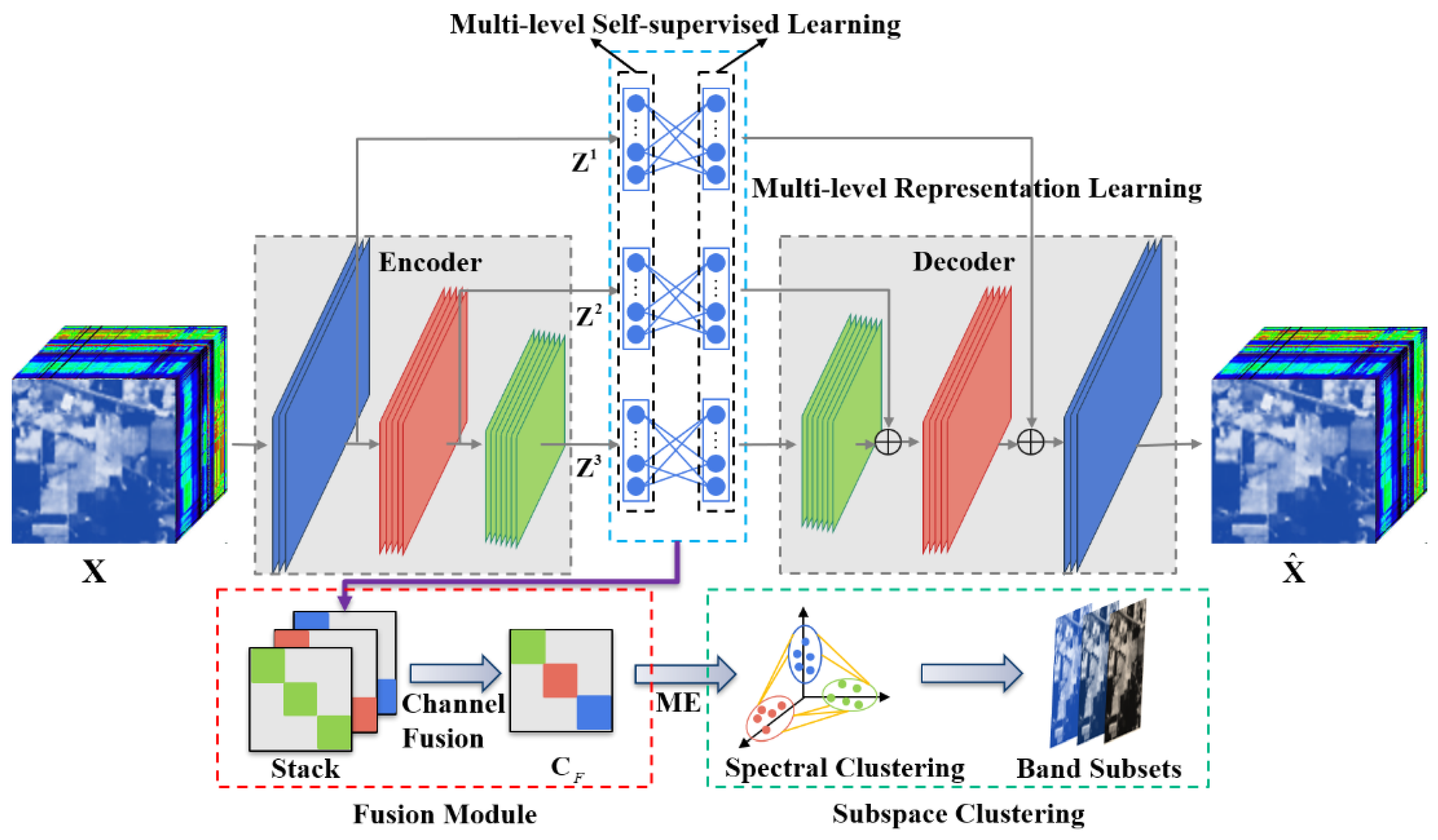
This section describes in detail the proposed MLRLFMESC method for BS. The flowchart of this method is shown in Figure 1. The main steps are as follows: firstly, considering the low-level and high-level spatial information of hyperspectral data, the proposed method inserts multiple fully connected layers between the encoder layers and their corresponding decoder layers to achieve multi-level representation learning (MLRL), thus generating multiple sets of self-expression coefficient matrices at different levels of the encoder layers to obtain more informative and discriminative subspace clustering representations. Secondly, a new auxiliary task is constructed based on the MLRL, which provides multi-level self-supervised information to further enhance the representation ability of the model, termed multi-level self-supervision learning (MLSL). Finally, a fusion module is designed to integrate the multi-scale information extracted from different layers of representation learning to obtain a more differentiated self-expression coefficient matrix, where maximum entropy regularization (MER) is introduced to ensure that elements of the same subspace are evenly and densely distributed, thereby enhancing connectivity within each subspace and facilitating subsequent spectral clustering to determine the most representative band subset.
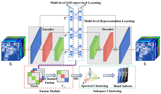
Figure 1.
Overall flowchart of the proposed MLRLFMESC framework.
2.1. Multi-Level Representation Learning (MLRL)
The proposed MLRLFMESC method exploits a deep stacked convolutional autoencoder (SCAE) constructed by the structure of a symmetrical encoder–decoder as the core network for feature extraction to sufficiently extract the spectral–spatial information of HSI data. The original HSI data cube contains W × H spatial dimensions and B spectral band dimensions. To ensure that the input of HSI samples X can be constructed by the deep SCAE, the definition of the loss of function is as follows:
where the Frobenius norm is expressed as , and the reconstructed HSI samples are denoted as .
Self-representation-based subspace clustering assumes that all data points belong to a combination of linear or affinity subspaces, which is typically represented as a self-representative model. Let the spectral bands come from the union of n different subspaces with the dimension in . In order to extract spatial information, considering the nonlinear relationships of HSI, the self-representative model is embedded in the latent space of the deep SCAE to implement self-representation properties and obtain representations of subspace clustering; then, the potential clusters are recovered with spectral clustering.
Inspired by the fact that the encoder with different layers can learn more complicated feature representations of the input HSI data, a self-representation model, comprising multiple fully connected layers, is inserted between the encoder layers of the deep stacked convolutional autoencoder and its corresponding decoder layers, respectively, to achieve MLRL; thus, the multi-level spectral–spatial information can be extracted. In order to capture the shared information between encoders and generate unique information for each layer, the consistency matrix and the discrimination matrix are defined, respectively. In view of the above-mentioned consideration, MLRL can be performed by the following loss function:
where represents the latent representation matrix and m is the dimension of the deep spatial feature.
The loss of self-expression is used to promote the learning of self-expression feature representations at different encoder levels. As for the discrimination matrix , the Frobenius norm is employed; thus, the connectivity of subspace representations related to each fully connected layer can be ensured. Meanwhile, to generate the sparse representation of the HSI, the l1-norm is used in the consistency matrix . Accordingly, the regular terms added to the model are shown as follows:
The multi-level spectral–spatial information of HSI is obtained via MLRL to facilitate the feature learning process, thereby obtaining multiple sets of information representations accordingly.
2.2. Multi-Level Self-Supervised Learning (MLSL)
Aiming at the further improvement of the representation ability of the proposed model, MLSL is used as a self-supervised method to better learn self-expression feature representations by constructing auxiliary tasks for MLRL.
To perform MLSL, the auxiliary tasks are constructed as follows: Firstly, positive and negative sample pairs are formulated for the inputs and outputs of the MLRL. For a given input and its corresponding set of outputs at layer l of MLRL, and are matched as a positive pair, while and are treated as a negative pair. Subsequently, the MLSL is implemented by formulating a self-supervised loss function, expressed as follows:
where σ is a temperature parameter that controls the distribution of the concentration level. and are normalizations of and , respectively.
An l2-normalization layer is used to satisfy and . The classifier of B-way softmax is exploited to classify as in the loss function of MLRL.
2.3. Fusion Module with Maximum Entropy Regularization (MER)
Considering that the coefficient matrices of the information representations obtained from MLRL have multiple information of the input HSI data, it is preferable to fuse these matrices into a more discriminative and informative coefficient subspace representation matrix as the input of the subspace clustering.
The matrices and learned using MLRL are fused through the fusion module. Stacking and along the channel dimension can help acquire the stacked matrix . Then, the channels of are merged using a convolutional kernel k to realize the fusion. Finally, a more informative subspace representation matrix is obtained via channel fusion learning, expressed as follows:
where is the convolution operation.
By using an appropriate kernel size k, is able to capture more local information on and each with the block diagonal structure.
Entropy is a measure of uncertain information contained within a random variable, where for a discrete random variable X, the entropy can be calculated as with p(X) as the probability distribution function of X. The similarity between hyperspectral data samples i and j in the subspace representation matrix can be expressed as , and the MER method is applied to the subspace representation matrix. According to the fact that , the following loss function for can be obtained as follows:
where satisfies . The MER forces the equal strength of connections between elements from the same subspace. Simultaneously, it ensures a uniform dense distribution of elements belonging to the same subspace.
2.4. Implementation Details
The final loss function of the proposed MLRLFMESC method is expressed as follows:
where are parameters that balance the trade-off between the earlier-mentioned different losses. and are the parameters updated by the standard backpropagation of the network trained with the Adam gradient.
Once the network has been trained to obtain the matrix , a symmetric affinity matrix can be created for spectral clustering,
Matrix A shows the pairwise relationship between the bands. Given the above, the spectral clustering algorithms can be utilized to recover the underlying subspaces and cluster the samples into respective subspaces to obtain the clustering results. The clustering centers can be obtained via the average of the spectrum in each cluster. Then, the distances between the cluster center and each band in the same cluster can be calculated to find the closest band as the selected representative band of the cluster, and the final subset of bands can be obtained.
3. Experiments and Results
3.1. Hyperspectral Datasets
Comparative experiments are conducted on three publicly available HSIs with different scenarios to prove the effectiveness of the proposed algorithm, including the Indian Pines (IP) dataset, the Pavia University (PU) dataset, and the Salinas (SA) dataset. Detailed descriptions of the three hyperspectral datasets are given in Table 1.

Table 1.
Descriptions of three HIS datasets.
3.1.1. Indian Pines (IP) Dataset
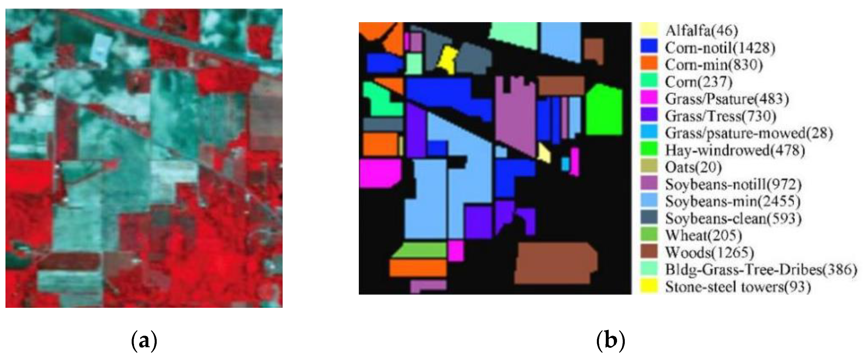
The IP dataset was captured using the AVIRIS sensor in Northwestern Indiana on 12 June 1992, containing 220 spectral bands with wavelengths of 0.4 to 2.5 μm and containing 145 × 145 pixels with a spatial resolution of 20 m. After the removal of 20 water absorption bands, 200 bands with 16 classes of crops are left for experiments. Figure 2 shows the IP dataset’s pseudo-color map as well as the true image feature class distribution.
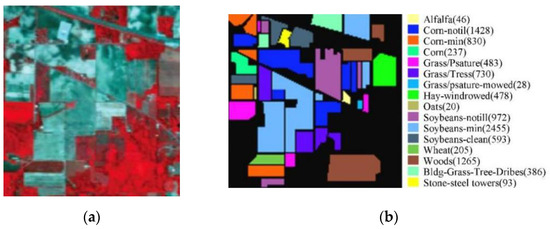
Figure 2.
The IP dataset with (a) a pseudo-color map of IP, and (b) true image class distribution with labels.
3.1.2. Pavia University (PU) Dataset
The PU dataset was collected via the ROSIS sensor for the city of Pavia in North Italy during a flying activity in 2003, consisting of 115 bands with wavelengths of 0.43 to 0.86 μm and containing 610 × 340 pixels with a spatial resolution of 1.3 m. After the removal of 12 noise bands, there are 9 types of objects available in the remaining 103 bands (the types of objects are shown in the label of Figure 3). The pseudo-color map and real image feature class distribution of the PU dataset are shown in Figure 3.
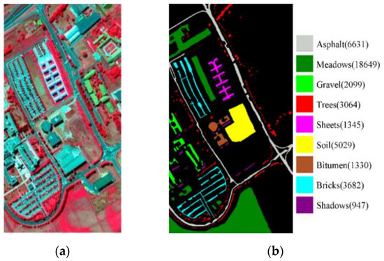
Figure 3.
The PU dataset, with (a) a pseudo-color map of PU, and (b) true image class distribution with labels.
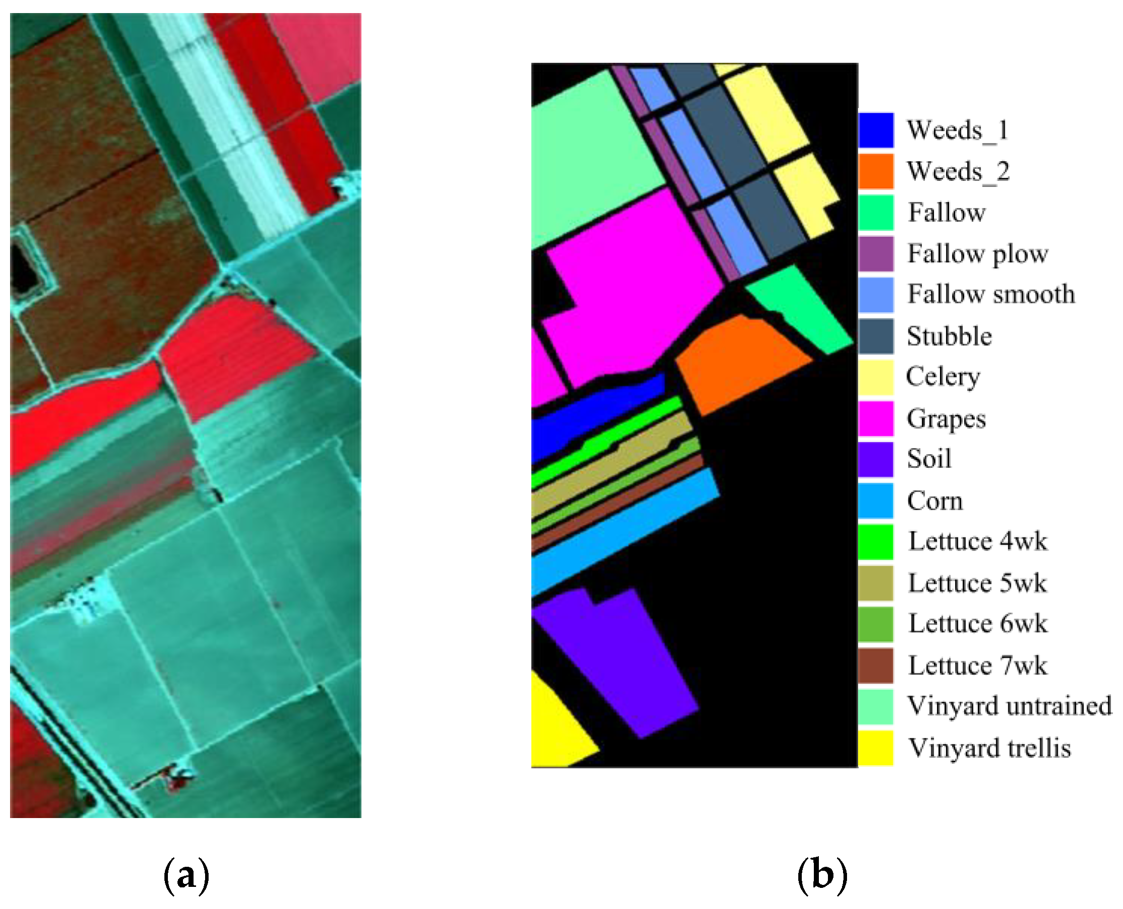
3.1.3. Salinas (SA) Dataset
The SA dataset was gathered using the AVIRIS sensor in Salinas Valley, California, in 1998, which comprises 224 bands with wavelengths of 0.36 to 2.5 µm and contains 512 × 217 pixels with spatial resolution of 3.7 m. After deleting 20 water absorption bands, the remaining 204 bands containing 16 classes are utilized for experiments. The pseudo-color map and real image feature class distribution of the SA dataset are shown in Figure 4.

Figure 4.
The SA dataset, with (a) a pseudo-color map of SA, and (b) true image class distribution with labels.
3.2. Experimental Setup
In order to prove the effectiveness of the proposed BS algorithm, five existing BS methods are used for comparison. Considering search-based, clustering-based, and ranking-based, as well as the comparison between traditional methods and deep learning methods, the selected comparable algorithms are UBS [18], E-FDPC [19], ISSC [25], ASPS_MN [5] and DSC [32], as these algorithms have open-source implementations provided by their respective authors. Performance analysis is conducted on a subset of bands obtained from various BS approaches using the same SVM classifier in [36] with an open-source code.
To quantitatively assess the quality of the selected band subsets, indicators of classification accuracy are used in this section, including overall accuracy (OA), average accuracy (AA), and the kappa coefficient (Kappa). For a fair comparative purpose, identical training and testing data subsets within each round are utilized when evaluating different BS algorithms. Specifically, 10% of samples from each class are randomly chosen as the training set, with the remaining samples allocated to the testing set. The experimental results are averaged via ten independent runs to reduce the randomness.
The deep SCAE network of the proposed method is composed of three symmetric layers of the stacked encoder and decoder with the following parameter settings: the stacked encoder consists of 10, 20, and 30 filters with corresponding kernel sizes of 5 × 5, 3 × 3, and 3 × 3, respectively. The network learning rate is The trade-off parameters are , , , and . The kernel size k is 3 × 3.
3.3. Randomness Validation by Random Selection of Training and Testing Sets
As for classification results, the training and testing sets have a significant influence on the classification performance. Therefore, before the comparison of various algorithms, this section gives the average and variance of OA across 10 distinct runs, allowing the assessment of disparities between experiment runs where each run involves alterations to the training and testing sets.
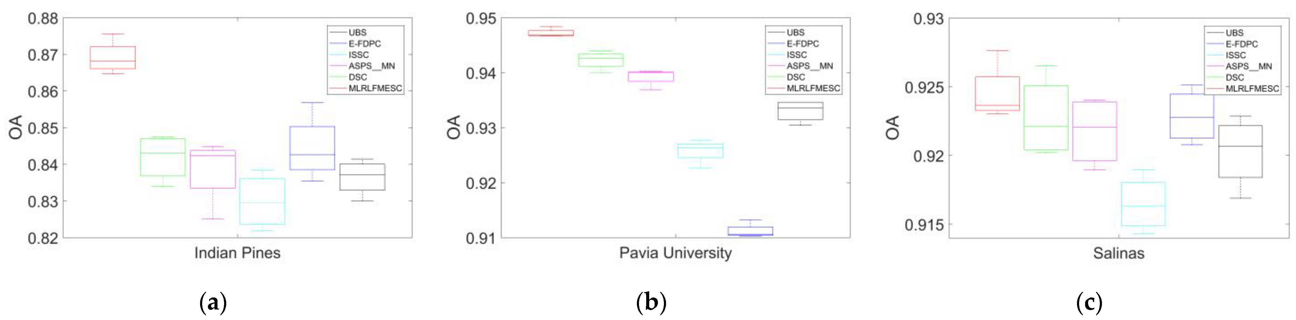
Figure 5a–c illustrates the box plots depicting the OA results for the six algorithms utilizing 35 bands across the three HSI datasets in 10 separate runs. The experiments entail the repeated random selection of training and testing datasets. To ensure an equitable comparison, the training and testing sets for all six algorithms within the same round remain identical. Sub-figures demonstrate that the proposed MLRLFMESC obtains the optimal mean OA with a perfect criteria bias, especially for IP and PU datasets, as shown in Figure 5a–c.

Figure 5.
Box plot of the OA for different BS methods on three hyperspectral datasets. (a) Indian Pines, (b) Pavia University, and (c) Salinas.
3.4. Ablation Study of the Proposed MLRLFMESC Method
To separately verify the effectiveness of maximum entropy regularization and self-supervised learning in the proposed MLRLFMESC method, ablation studies are conducted in this section. As can be shown in Equation (8) in Section 2, the proposed method adopts partial loss functions from the DSC method, namely , , , and , collectively referred to as in this paper. Building upon this foundation, the proposed method introduces the following two innovative techniques: the multi-level self-supervised learning model (MLSL) and maximum entropy regularization (MER). In MLSL, the is introduced to obtain improved self-supervised features. In MER, the is introduced to promote connectivity within the same subspace while ensuring a uniform and dense distribution of elements within the subspace, which is beneficial for subsequent spectral clustering. As a result, the ablation study should be implemented with/without the and the loss in Table 2.
Table 2.
Ablation study for maximum entropy regularization and self-supervised learning.
The following conclusions are given from Table 2: Firstly, when adding either the MER into the model (as shown in the second line in Table with the form of ) or the multi-level self-supervised learning model (as shown in the third line in the Table with the form of ), the OA performance can be better than the DSC method. The classification performance of the proposed MLRLFMESC with both MER and MLSL (as shown in the fourth line in Table with the form of and ) has the best OA performance with bold fonts under the selection with a different number of selected band subsets. These experiments demonstrate the effectiveness of maximum entropy regularization and self-supervised learning in the proposed MLRLFMESC approach.
3.5. Classification Results Analysis for Different BS Algorithms
In this section, comparative experiments are conducted on three publicly available HSIs with different scenarios to prove the effectiveness of the proposed algorithm, including the Indian Pines (IP) dataset, the Pavia University (PU) dataset, and the Salinas (SA) dataset. However, limited by the number of pages and considering the reproducibility of conclusions, only the results of the IP dataset are shown in this section, with the results of the PU and SA datasets in Appendix A and Appendix B.
3.5.1. BS Results with Different Number of Selected Bands
To evaluate the classification accuracy of the proposed MLRLFMESC algorithm while comparing it with the existing BS methods, the quantity n of selected bands in different BS methods is varied in the region of [5,35] with a step of five. The reason why we chose 35 as the maximum is that when using virtual dimension (VD) analysis, which is a widely used technique for selecting the number of bands, the VD is typically less than 35.
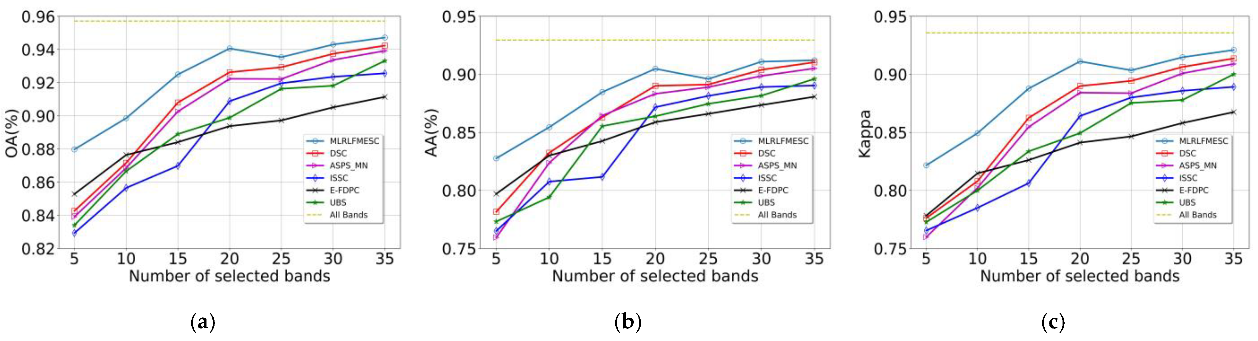
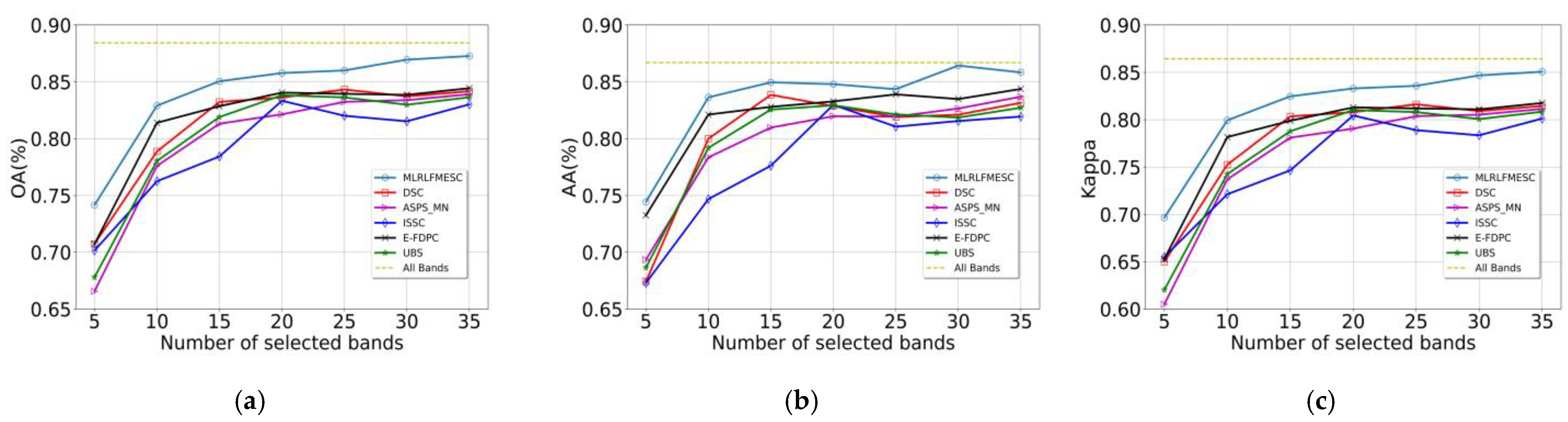
In Figure 6, the suggested MLRLFMESC technique clearly outperforms the other five BS approaches in terms of classification accuracy for OA, AA, and Kappa. In Figure 6a of the IP dataset, the proposed MLRLFMESC has the highest and most stable OA with a significant improvement over the other five comparable BS methods, especially when n = 5, 30, 35, and the proposed MLRLFMESC has better accuracies of 3.42%, 3.56%, and 2.83% compared to the suboptimal approach. The AA accuracy is shown in Figure 6b, and the MLRLFMESC technique exhibits the “Hughes” phenomena that grows and then drops as the number of bands increases. In terms of the Kappa given in Figure 6c, the MLRLFMESC approach has a growing advantage over the suboptimal approach as the number of chosen bands grows, notably when n = 30, 35, MLRLFMESC has 3.56% and 2.83% greater accuracy than the suboptimal approach, respectively. The other five BS approaches exhibit some “Hughes” phenomena in the OA, AA, and Kappa curves, indicating the necessity for band selection.
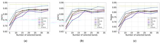
Figure 6.
Classification performance with a different number of selected bands on IP, (a) OA, (b) AA, (c) Kappa.
3.5.2. Classification Performance Analysis by Band Subsets Using Various BS Algorithms
To further assess the efficacy of the proposed MLRLFMESC approach for the analysis, Figure 7 shows the index distribution of the 30 bands selected from the IP dataset via various band selection approaches. It is usually regarded as a bad strategy if the selected bands are scattered across a relatively short range.
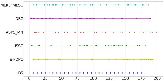
Figure 7.
Distribution of bands selected using various BS algorithms on IP data.
As can be seen in Figure 7, most band selection approaches pick bands that span a broad range of all bands.
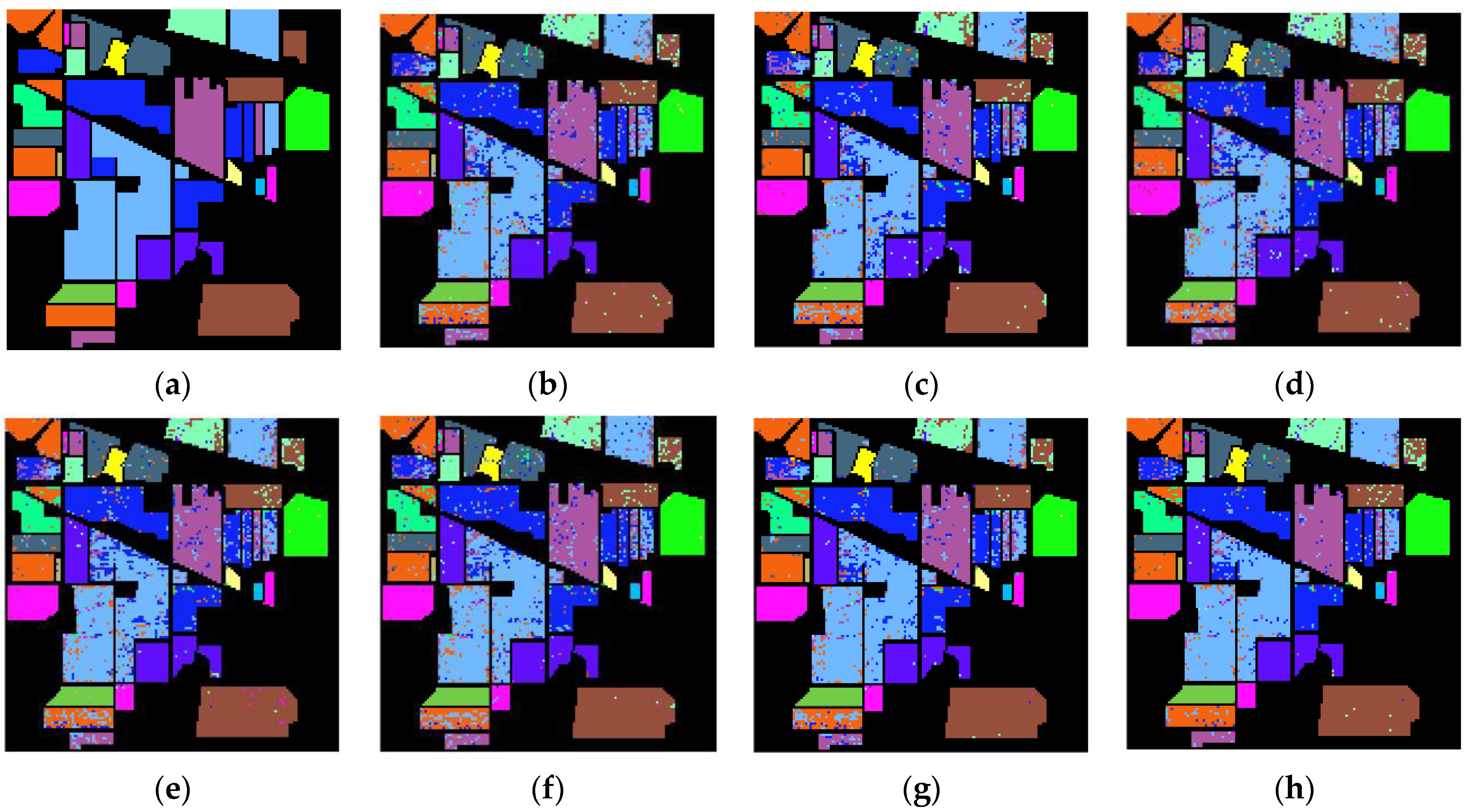
Figure 8 presents the labeled image, the classification result maps for the various band selection methods, and all bands, which may be used to visually analyze the classification performance of various band selection methods on the IP dataset. There is some visual deviance, especially regarding the fact that the proposed algorithm has the best performance of the corn-min class with the orange color in the lower left corner and the better performance of the wood class with the brown color in the lower right corner. Further quantitative analysis is conducted for a fair comparison.
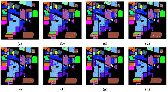
Figure 8.
Classification result maps, (a) labeled image, and (b–h) classification result maps on IP-selected 30 bands using UBS, E-FDPC, ISSC, ASPS_MN, DSC, MLRLFMESC, and all bands, respectively.
In order for a quantitative comparison, Table 3 displays the average classification results of 10 runs with OA, AA, and Kappa, using various band selection methods (UBS, E-FDPC, ISSC, ASPS_MN, DSC, and the proposed MLRLFMESC, respectively) and all bands, where the best classification results are blacked out and the second-best results are underlined.
Table 3.
Comparison of classification results from various BS approaches on the IP dataset.
It can be easily seen from Table 3 that the proposed method outperforms all previous band selection methods except all bands in terms of OA, AA, and Kappa, as well as classification accuracy in most classes. The proposed MLRLFMESC approach provides the highest classification accuracy in classes 8, 12, and 15 when compared to existing approaches.
3.6. Time Consuming for Different BS Algorithms
In this section, a comparison of computing times across different band selection algorithms is conducted to discern their respective computational complexity. Table 4 lists the average computation time for ten runs of various BS approaches on the IP dataset, where the ISSC has the lowest running time with bold font. Since MLRLFMESC and DSC use deep neural networks, the running time is longer compared to traditional BS methods. However, the runtime of MLRLFMESC is significantly less than that of DSC, efficiently obtaining the desired bands within an acceptable timeframe while achieving a superior classification performance.
Table 4.
Comparison of time consumption from various BS approaches on the IP dataset.
4. Conclusions and Discussion
This paper presents a novel MLRLFMESC framework for unsupervised hyperspectral band selection. Self-representation subspace clustering is applied in deep SCAE to enable the learning of hyperspectral nonlinear spectra–spatial relationships in a trainable deep network.
- (1)
- From the results in Section 3, it can be seen that the proposed MLSL model retains good band subsets with multi-level spectral–spatial information and multi-level discriminative information representations.
- (2)
- A fusion module is employed to fuse the multi-level discriminative information representations, where the MER method is applied to enhance the objectiveness of the bands in each subspace while ensuring the uniform and dense distribution of bands in the same subspace, which was shown to be successful in the ablation study.
- (3)
- Comparable experiments indicate that the proposed MLRLFMESC approach performs better than the other five state-of-the-art BS methods on three real HSI datasets for classification performance.
Although this work, and even other existing BS methods, have been extensively studied and achieved excellent performance in classification tasks, there has been limited research on integrating BS algorithms into tasks such as hyperspectral image target detection, target tracking, unmixing, etc. An important research direction in the future is to apply band selection algorithms to different task requirements while considering high performance. Furthermore, this paper does not pay attention to the problem of the uneven distribution of samples in classification-oriented tasks, resulting in the better performance of large categories and the poor performance of small categories. Therefore, the expansion of small category samples and the design or improvement of targeted models are the direction of focus in further research.
Author Contributions
Conceptualization, Y.W.; methodology, Y.W. and H.M.; software, H.M. and Y.Y.; validation, E.Z., M.S. and C.Y.; formal analysis, Y.W.; investigation, H.M.; data curation, H.M. and Y.Y.; writing—original draft preparation, Y.W. and H.M.; writing—review and editing, Y.W. All authors have read and agreed to the published version of the manuscript.
Funding
This research was supported in part by the National Nature Science Foundation of China under Grant 42271355 and Grant 61801075, in part by the Natural Science Foundation of Liaoning Province under Grant 2022-MS-160, in part by the China Postdoctoral Science Foundation under Grant 2020M670723, and in part by the Fundamental Research Funds for the Central Universities under Grant 3132023238.
Data Availability Statement
Data are contained within this article. The source code of the proposed algorithm will be available at https://github.com/YuleiWang1.
Acknowledgments
We would like to thank the authors of the compared algorithms for their open-source codes.
Conflicts of Interest
The authors declare no conflicts of interest.
Appendix A. BS Results and Analysis for PU
In this appendix, the performance of different BS algorithms is compared using the PU dataset.
As shown in Figure A1, the OA, AA, and Kappa curves generated via various BS approaches with varying numbers of bands selected on the PU dataset are computed and recorded. The proposed MLRLFMESC method’s performance for OA, AA, and Kappa initially and gradually improves as selected bands grow, then shows a downward trend from n = 20 to n = 25, followed by an upward trend; this is the behavior known as the “Hughes” phenomenon. The proposed MLRLFMESC algorithm wins over the other five comparable BS methods with a significant classification priority in terms of OA, AA, and Kappa performance on the PU dataset, as illustrated in Figure A1, especially when n = 5, 10, 15, 20, and the OA, AA, and Kappa values have a clear advantage compared to the sub-optimal approach.
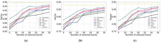
Figure A1.
Classification performance of PU dataset with a different number of selected bands, (a) OA, (b) AA, (c) Kappa.
Figure A1.
Classification performance of PU dataset with a different number of selected bands, (a) OA, (b) AA, (c) Kappa.
The index distribution of the six band selection algorithms for selecting 20 bands of the PU dataset is shown in Figure A2. The selected bands are distributed widely and discretely in the proposed MLRLFMESC algorithm.

Figure A2.
Distribution of bands selected using various BS algorithms for PU dataset.
Figure A2.
Distribution of bands selected using various BS algorithms for PU dataset.
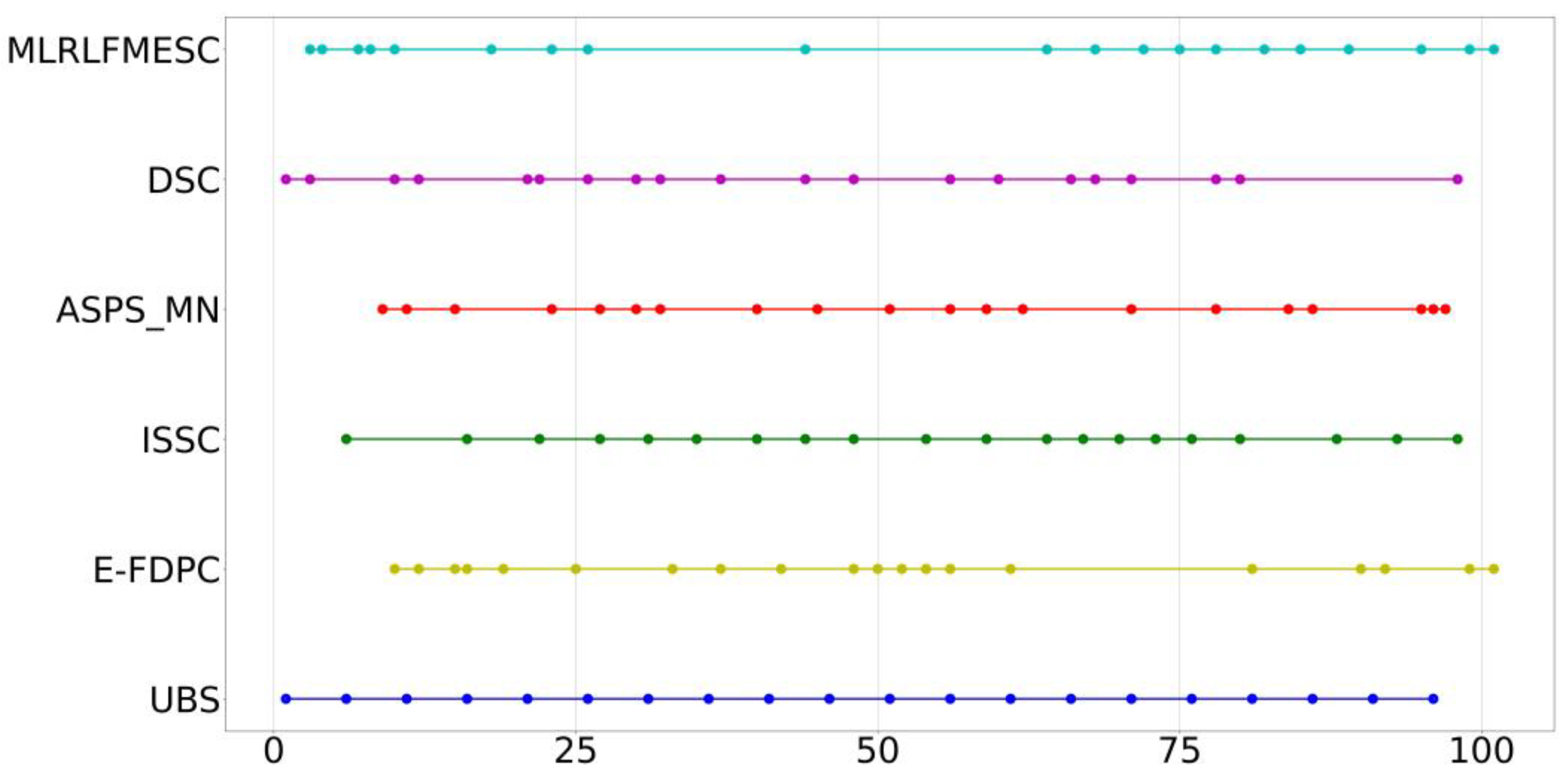
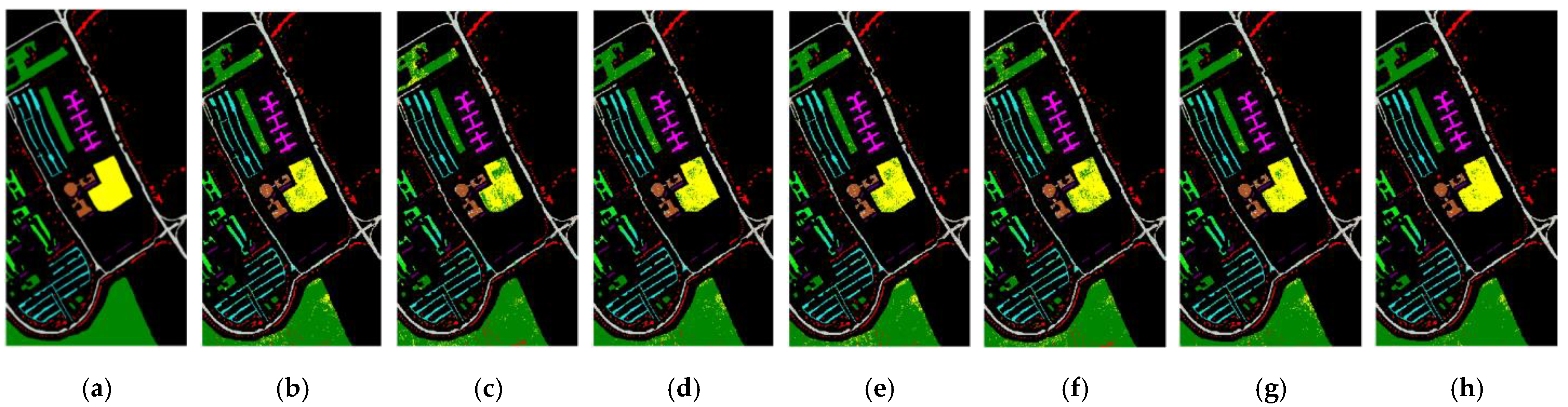
Figure A3 shows the real label image, the visual classification maps for six BS methods and 20 selected bands, and full bands on the PU dataset, illustrating that the classification maps contain many misclassified samples, and the proposed MLRLFMESC method has a slightly better classification result map than the other five BS methods.
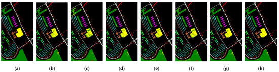
Figure A3.
Classification result maps with (a) a labeled image of PU, and (b–h) classification result maps with 20 bands using UBS, E-FDPC, ISSC, ASPS_MN, DSC, MLRLFMESC, and all bands.
Figure A3.
Classification result maps with (a) a labeled image of PU, and (b–h) classification result maps with 20 bands using UBS, E-FDPC, ISSC, ASPS_MN, DSC, MLRLFMESC, and all bands.
The same comparison is conducted for the PU dataset to quantitatively compare the performance of different BS algorithms, where the average classification results for all bands and all 20 BS algorithm-selected 20 bands are listed in Table A1 using OA, AA, and Kappa performance. The best values of OA, AA, and Kappa in each category are blacked out, and the second-best values are underlined. It can be seen that the proposed MLRLFMESC algorithm achieves the highest classification accuracy in most categories, except for all bands. Compared with the DSC algorithm, the MLRLFMESC algorithm exhibits 1.43%, 1.47%, and 2.13% improvements in OA, AA, and Kappa, respectively.
Table A1.
Comparison of classification results from various BS approaches on the PU dataset.
Table A1.
Comparison of classification results from various BS approaches on the PU dataset.
| Algorithms | UBS | E-FDPC | ISSC | ASPS_MN | DSC | MLRLFMESC | All Bands |
|---|---|---|---|---|---|---|---|
| OA | 89.88 ± 0.50 | 89.38 ± 0.94 | 90.88 ± 0.49 | 92.23 ± 0.36 | 92.63 ± 0.21 | 94.06 ± 0.38 | 95.71 ± 0.31 |
| AA | 86.39 ± 0.71 | 85.88 ± 1.13 | 87.17 ± 0.74 | 88.33 ± 0.54 | 89.01 ± 0.43 | 90.48 ± 0.56 | 92.95 ± 0.82 |
| Kappa | 84.94 ± 0.66 | 84.12 ± 1.32 | 86.41 ± 0.73 | 88.42 ± 0.57 | 88.99 ± 0.37 | 91.12 ± 0.55 | 93.57 ± 0.43 |
| 1 | 96.10 ± 0.56 | 95.85 ± 1.00 | 95.88 ± 0.72 | 96.16 ± 0.90 | 96.23 ± 0.81 | 96.70 ± 0.74 | 97.23 ± 0.63 |
| 2 | 95.16 ± 0.45 | 94.40 ± 0.36 | 96.01 ± 0.60 | 97.15 ± 0.38 | 97.19 ± 0.55 | 98.09 ± 0.55 | 98.82 ± 0.23 |
| 3 | 77.67 ± 4.26 | 75.45 ± 4.22 | 78.62 ± 2.46 | 80.28 ± 3.50 | 80.86 ± 2.74 | 82.85 ± 2.36 | 87.37 ± 3.99 |
| 4 | 82.13 ± 4.74 | 85.88 ± 2.95 | 85.77 ± 3.82 | 90.16 ± 3.63 | 90.81 ± 2.41 | 91.85 ± 3.03 | 94.10 ± 2.87 |
| 5 | 99.81 ± 0.53 | 99.79 ± 0.53 | 99.79 ± 0.36 | 99.82 ± 0.35 | 99.80 ± 0.70 | 99.77 ± 0.54 | 99.87 ± 0.19 |
| 6 | 70.20 ± 4.49 | 68.49 ± 7.46 | 73.34 ± 4.82 | 77.17 ± 3.77 | 78.36 ± 2.08 | 83.61 ± 2.06 | 88.14 ± 1.43 |
| 7 | 76.76 ± 4.18 | 74.60 ± 4.47 | 74.86 ± 5.72 | 73.81 ± 3.12 | 76.65 ± 2.89 | 79.09 ± 5.35 | 85.05 ± 4.85 |
| 8 | 79.70 ± 2.78 | 78.50 ± 1.93 | 80.32 ± 2.67 | 80.47 ± 2.02 | 81.19 ± 2.34 | 82.47 ± 1.53 | 86.00 ± 2.60 |
| 9 | 100.00 ± 0.00 | 100.00 ± 0.00 | 99.97 ± 0.25 | 99.92 ± 0.25 | 100.00 ± 0.00 | 99.90 ± 0.50 | 99.95 ± 0.25 |
Appendix B. BS Results and Analysis for SA
In this appendix, the performance of different BS algorithms is compared using the SA dataset.
Figure A4 compares the classification curves for the proposed MLRLFMESC method and alternative BS methods selecting different numbers of bands, as well as the classification performance of all bands. For the SA dataset, the proposed MLRLFMESC algorithm shows the stable and best OA and Kappa accuracy performance when compared to the other five comparable BS methods, as seen in Figure A4; as n increases, the proposed MLRLFMESC method gradually increases in terms of the OA and Kappa performance. Notably, when n = 15, E-FDPC outperforms MLRLFMESC in terms of AA, and MLRLFMESC outperforms ASPS_MN in terms of AA when n = 20. However, the MLRLFMESC method outperforms the other five methods in terms of the AA performance for the majority of selected bands.
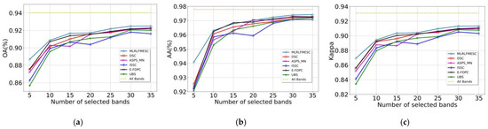
Figure A4.
Classification performance of SA dataset with a different number of selected bands, (a) OA, (b) AA, (c) Kappa.
Figure A4.
Classification performance of SA dataset with a different number of selected bands, (a) OA, (b) AA, (c) Kappa.
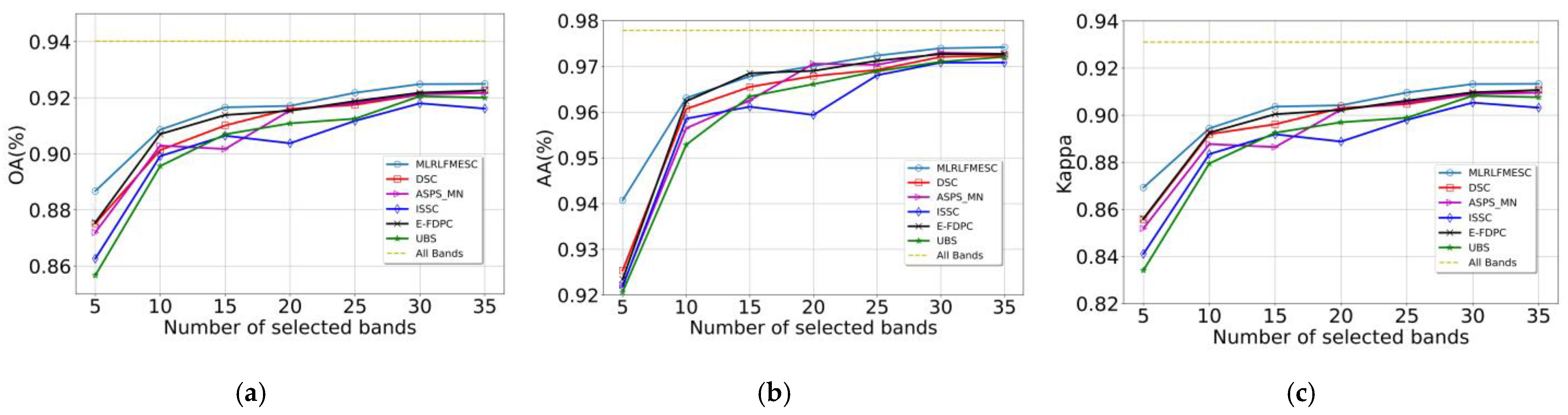
Figure A5 provides the index distribution of the six band selection methods with 30 bands selected, where similar conclusions can be given as IP and PU datasets.
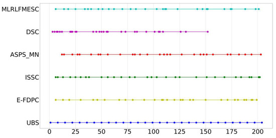
Figure A5.
Distribution of bands selected using various BS algorithms for SA dataset.
Figure A5.
Distribution of bands selected using various BS algorithms for SA dataset.

Figure A6 shows the true label image and the classification result maps for six BS methods, selecting 30 bands and all bands on the SA dataset. The visual map of the classification results shows that all bands and the other six methods have several clear misclassifications. All bands maintain better regional consistency and provide a visualization closer to the ground truth.
The quantitative average classification results of all BS algorithms for 30 bands and all bands are shown in Table A2, with the best results blacked out and the second-best results underlined. Compared with DSC, MLRLFMESC has a slightly higher OA, AA, and Kappa accuracy. For each category of accuracy, all BS methods achieved a performance of 98% or above except for categories 8 and 15, and the proposed MLRLFMESC approach achieved the best category accuracy in categories 8 and 15 compared to the other five approaches.
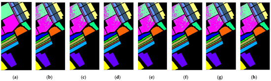
Figure A6.
Classification result maps with a (a) labeled image of SA, and (b–h) classification result maps with 30 bands using UBS, E-FDPC, ISSC, ASPS_MN, DSC, MLRLFMESC, and all bands.
Figure A6.
Classification result maps with a (a) labeled image of SA, and (b–h) classification result maps with 30 bands using UBS, E-FDPC, ISSC, ASPS_MN, DSC, MLRLFMESC, and all bands.
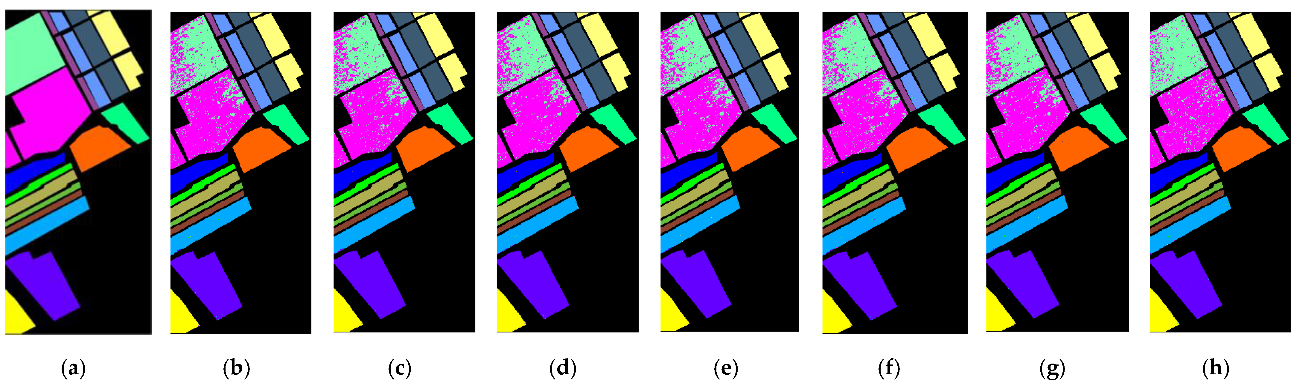
Table A2.
Comparison of classification results from various BS approaches on SA dataset.
Table A2.
Comparison of classification results from various BS approaches on SA dataset.
| Algorithms | UBS | E-FDPC | ISSC | ASPS_MN | DSC | MLRLFMESC | All Bands |
|---|---|---|---|---|---|---|---|
| OA | 92.05 ± 0.85 | 92.18 ± 0.50 | 91.80 ± 0.62 | 92.12 ± 0.53 | 92.11 ± 0.56 | 92.49 ± 0.73 | 94.02 ± 0.35 |
| AA | 97.10 ± 0.44 | 97.27 ± 0.32 | 97.08 ± 0.39 | 97.30 ± 0.33 | 97.21 ± 0.23 | 97.40 ± 0.32 | 97.79 ± 0.21 |
| Kappa | 90.83 ± 0.98 | 90.97 ± 0.59 | 90.53 ± 0.69 | 90.90 ± 0.62 | 90.89 ± 0.64 | 91.32 ± 0.84 | 93.10 ± 0.41 |
| 1 | 100.00 ± 0.00 | 99.92 ± 0.12 | 99.98 ± 0.12 | 99.95 ± 0.12 | 99.97 ± 0.23 | 99.99 ± 0.12 | 99.95 ± 0.12 |
| 2 | 99.92 ± 0.24 | 99.92 ± 0.19 | 99.88 ± 0.34 | 99.92 ± 0.24 | 99.92 ± 0.29 | 99.95 ± 0.19 | 99.95 ± 0.24 |
| 3 | 99.04 ± 1.27 | 99.80 ± 0.70 | 99.68 ± 0.47 | 99.76 ± 0.57 | 99.61 ± 0.80 | 99.78 ± 0.80 | 99.87 ± 0.34 |
| 4 | 99.36 ± 0.99 | 99.44 ± 0.99 | 99.45 ± 0.97 | 99.43 ± 1.30 | 99.38 ± 0.83 | 99.49 ± 0.98 | 99.38 ± 1.14 |
| 5 | 99.01 ± 1.53 | 99.50 ± 0.86 | 99.48 ± 0.77 | 99.48 ± 1.02 | 99.46 ± 1.28 | 99.50 ± 1.11 | 99.53 ± 1.03 |
| 6 | 99.97 ± 0.13 | 99.96 ± 0.13 | 99.96 ± 0.09 | 99.94 ± 0.18 | 99.96 ± 0.13 | 99.96 ± 0.09 | 99.96 ± 0.13 |
| 7 | 99.97 ± 0.05 | 99.98 ± 0.05 | 99.99 ± 0.05 | 99.94 ± 0.21 | 99.96 ± 0.10 | 99.99 ± 0.10 | 99.97 ± 0.15 |
| 8 | 84.46 ± 2.67 | 84.34 ± 2.59 | 83.56 ± 1.67 | 83.95 ± 2.49 | 84.48 ± 2.40 | 84.73 ± 2.59 | 89.96 ± 1.57 |
| 9 | 99.67 ± 0.14 | 99.67 ± 0.19 | 99.62 ± 0.26 | 99.65 ± 0.14 | 99.68 ± 0.17 | 99.73 ± 0.19 | 99.73 ± 0.21 |
| 10 | 98.07 ± 1.22 | 98.71 ± 0.88 | 98.38 ± 1.48 | 98.48 ± 1.55 | 98.52 ± 1.11 | 98.58 ± 0.65 | 98.37 ± 1.29 |
| 11 | 98.86 ± 2.08 | 99.23 ± 0.85 | 98.56 ± 1.91 | 99.94 ± 0.22 | 99.36 ± 1.69 | 99.21 ± 1.06 | 99.62 ± 1.48 |
| 12 | 99.71 ± 0.70 | 99.61 ± 0.81 | 99.78 ± 0.70 | 99.64 ± 0.59 | 99.62 ± 0.83 | 99.62 ± 1.16 | 99.69 ± 0.47 |
| 13 | 99.67 ± 0.78 | 99.80 ± 0.51 | 99.75 ± 0.78 | 99.90 ± 0.52 | 99.75 ± 0.74 | 99.95 ± 0.26 | 99.80 ± 0.51 |
| 14 | 98.84 ± 2.67 | 98.73 ± 2.86 | 98.69 ± 2.12 | 98.92 ± 2.67 | 98.57 ± 3.04 | 99.03 ± 1.86 | 98.52 ± 2.23 |
| 15 | 77.39 ± 2.79 | 77.88 ± 1.54 | 76.95 ± 3.71 | 78.14 ± 2.22 | 77.36 ± 2.30 | 79.08 ± 2.59 | 80.80 ± 1.78 |
| 16 | 99.68 ± 0.87 | 99.77 ± 0.63 | 99.62 ± 0.63 | 99.75 ± 0.51 | 99.75 ± 0.64 | 99.75 ± 0.77 | 99.47 ± 1.25 |
References
- Wang, J.; Liu, J.; Cui, J.; Luan, J.; Fu, Y. Multiscale fusion network based on global weighting for hyperspectral feature selection. IEEE J. Sel. Top. Appl. Earth Observ. Remote Sens. 2023, 16, 2977–2991. [Google Scholar] [CrossRef]
- Yu, C.; Zhou, S.; Song, M.; Gong, B.; Zhao, E.; Chang, C.-I. Unsupervised hyperspectral band selection via hybrid graph convolutional network. IEEE Trans. Geosci. Remote Sens. 2022, 60, 5530515. [Google Scholar] [CrossRef]
- Zhong, Y.; Wang, X.; Xu, Y.; Wang, S.; Jia, T.; Hu, X.; Zhao, J.; Wei, L.; Zhang, L. Mini-UAV-borne hyperspectral remote sensing: From observation and processing to applications. IEEE Geosci. Remote Sens. Mag. 2018, 6, 46–62. [Google Scholar] [CrossRef]
- Ghamisi, P.; Yokoya, N.; Li, J.; Liao, W.; Liu, S.; Plaza, J.; Rasti, B.; Plaza, A. Advances in hyperspectral image and signal processing: A comprehensive overview of the state of the art. IEEE Geosci. Remote Sens. Mag. 2017, 5, 37–78. [Google Scholar] [CrossRef]
- Wang, Q.; Li, Q.; Li, X. Hyperspectral band selection via adaptive subspace partition strategy. IEEE J. Sel. Top. Appl. Earth Observ. Remote Sens. 2019, 12, 4940–4950. [Google Scholar] [CrossRef]
- Li, S.; Liu, Z.; Fang, L.; Li, Q. Block diagonal representation learning for hyperspectral band selection. IEEE Trans. Geosci. Remote Sens. 2023, 61, 5509213. [Google Scholar] [CrossRef]
- Ma, M.; Mei, S.; Li, F.; Ge, Y.; Du, Q. Spectral correlation-based diverse band selection for hyperspectral image classification. IEEE Trans. Geosci. Remote Sens. 2023, 61, 5508013. [Google Scholar] [CrossRef]
- Deng, Y.-J.; Li, H.-C.; Tan, S.-Q.; Hou, J.; Du, Q.; Plaza, A. t-Linear tensor subspace learning for robust feature extraction of hyperspectral images. IEEE Trans. Geosci. Remote Sens. 2023, 61, 5501015. [Google Scholar] [CrossRef]
- Yu, W.; Huang, H.; Shen, G. Deep spectral–spatial feature fusion-based multiscale adaptable attention network for hyperspectral feature extraction. IEEE Trans. Instrum. Meas. 2023, 72, 5500813. [Google Scholar] [CrossRef]
- Ou, X.; Wu, M.; Tu, B.; Zhang, G.; Li, W. Multi-objective unsupervised band selection method for hyperspectral images classification. IEEE Trans. Image Process. 2023, 32, 1952–1965. [Google Scholar] [CrossRef]
- Li, S.; Peng, B.; Fang, L.; Zhang, Q.; Cheng, L.; Li, Q. Hyperspectral band selection via difference between intergroups. IEEE Trans. Geosci. Remote Sens. 2023, 61, 5503310. [Google Scholar] [CrossRef]
- Habermann, M.; Fremont, V.; Shiguemori, E.H. Supervised band selection in hyperspectral images using single-layer neural networks. Int. J. Remote Sens. 2019, 40, 3900–3926. [Google Scholar] [CrossRef]
- Esmaeili, M.; Abbasi-Moghadam, D.; Sharifi, A.; Tariq, A.; Li, Q. Hyperspectral image band selection based on CNN embedded GA (CNNeGA). IEEE J. Sel. Top. Appl. Earth Observ. Remote Sens. 2023, 16, 1927–1950. [Google Scholar] [CrossRef]
- Sun, W.; Yang, G.; Peng, J.; Du, Q. Hyperspectral band selection using weighted kernel regularization. IEEE J. Sel. Top. Appl. Earth Observ. Remote Sens. 2019, 12, 3665–3676. [Google Scholar] [CrossRef]
- Sellami, A.; Farah, I.R. A spatial hypergraph based semi-supervised band selection method for hyperspectral imagery semantic interpretation. Int. J. Comput. Inf. Eng. 2016, 10, 1839–1846. [Google Scholar]
- He, F.; Nie, F.; Wang, R.; Jia, W.; Zhang, F.; Li, X. Semisupervised band selection with graph optimization for hyperspectral image classification. IEEE Trans. Geosci. Remote Sens. 2021, 59, 10298–10311. [Google Scholar] [CrossRef]
- Cao, X.; Wei, C.; Ge, Y.; Feng, J.; Zhao, J.; Jiao, L. Semi-supervised hyperspectral band selection based on dynamic classifier selection. IEEE J. Sel. Top. Appl. Earth Observ. Remote Sens. 2019, 12, 1289–1298. [Google Scholar] [CrossRef]
- Chein, I.C.; Su, W. Constrained band selection for hyperspectral imagery. IEEE Trans. Geosci. Remote Sens. 2006, 44, 1575–1585. [Google Scholar] [CrossRef]
- Jia, S.; Tang, G.; Zhu, J.; Li, Q. A novel ranking-based clustering approach for hyperspectral band selection. IEEE Trans. Geosci. Remote Sens. 2016, 54, 88–102. [Google Scholar] [CrossRef]
- Fu, H.; Zhang, A.; Sun, G.; Ren, J.; Jia, X.; Pan, Z.; Ma, H. A novel band selection and spatial noise reduction method for hyperspectral image classification. IEEE Trans. Geosci. Remote Sens. 2022, 60, 5535713. [Google Scholar] [CrossRef]
- Ji, H.; Zuo, Z.; Han, Q.L. A divisive hierarchical clustering approach to hyperspectral band selection. IEEE Trans. Instrum. Meas. 2022, 71, 5014312. [Google Scholar] [CrossRef]
- Sun, W.; Tian, L.; Xu, Y.; Zhang, D.; Du, Q. Fast and robust self-representation method for hyperspectral band selection. IEEE J. Sel. Top. Appl. Earth Observ. Remote Sens. 2017, 10, 5087–5098. [Google Scholar] [CrossRef]
- Zhang, Y.; Wang, X.; Jiang, X.; Zhou, Y. Robust dual graph self-representation for unsupervised hyperspectral band selection. IEEE Trans. Geosci. Remote Sens. 2022, 60, 5538513. [Google Scholar] [CrossRef]
- Zhang, Y.; Wang, X.; Jiang, X.; Zhou, Y. Marginalized graph self-representation for unsupervised hyperspectral band selection. IEEE Trans. Geosci. Remote Sens. 2022, 60, 5516712. [Google Scholar] [CrossRef]
- Sun, W.; Zhang, L.; Du, B.; Li, W.; Lai, Y.M. Band selection using improved sparse subspace clustering for hyperspectral imagery classification. IEEE J. Sel. Top. Appl. Earth Observ. Remote Sens. 2015, 8, 2784–2797. [Google Scholar] [CrossRef]
- Zhai, H.; Zhang, H.; Zhang, L.; Li, P. Laplacian-regularized low-rank subspace clustering for hyperspectral image band selection. IEEE Trans. Geosci. Remote Sens. 2019, 57, 1723–1740. [Google Scholar] [CrossRef]
- Huang, S.; Zhang, H.; Pižurica, A. A structural subspace clustering approach for hyperspectral band selection. IEEE Trans. Geosci. Remote Sens. 2022, 60, 5509515. [Google Scholar] [CrossRef]
- Sun, H.; Ren, J.; Zhao, H.; Yuen, P.; Tschannerl, J. Novel gumbel-softmax trick enabled concrete autoencoder with entropy constraints for unsupervised hyperspectral band selection. IEEE Trans. Geosci. Remote Sens. 2022, 60, 5506413. [Google Scholar] [CrossRef]
- Zhang, H.; Sun, X.; Zhu, Y.; Xu, F.; Fu, X. A global-local spectral weight network based on attention for hyperspectral band selection. IEEE Geosci. Remote Sens. Lett. 2022, 19, 6004905. [Google Scholar] [CrossRef]
- Zhang, X.; Xie, W.; Li, Y.; Lei, J.; Du, Q.; Yang, G. Rank-aware generative adversarial network for hyperspectral band selection. IEEE Trans. Geosci. Remote Sens. 2022, 60, 5521812. [Google Scholar] [CrossRef]
- Feng, J.; Bai, G.; Li, D.; Zhang, X.; Shang, R.; Jiao, L. MR-selection: A meta-reinforcement learning approach for zero-shot hyperspectral band selection. IEEE Trans. Geosci. Remote Sens. 2023, 61, 5500320. [Google Scholar] [CrossRef]
- Zeng, M.; Cai, Y.; Cai, Z.; Liu, X.; Hu, P.; Ku, J. Unsupervised hyperspectral image band selection based on deep subspace clustering. IEEE Geosci. Remote Sens. Lett. 2019, 16, 1889–1893. [Google Scholar] [CrossRef]
- Das, S.; Pratiher, S.; Kyal, C.; Ghamisi, P. Sparsity regularized deep subspace clustering for multicriterion-based hyperspectral band selection. IEEE J. Sel. Top. Appl. Earth Observ. Remote Sens. 2022, 15, 4264–4278. [Google Scholar] [CrossRef]
- Dou, Z.; Gao, K.; Zhang, X.; Wang, H.; Han, L. Band selection of hyperspectral images using attention-based autoencoders. IEEE Geosci. Remote Sens. Lett. 2021, 18, 147–151. [Google Scholar] [CrossRef]
- Goel, A.; Majumdar, A. K-means embedded deep transform learning for hyperspectral band selection. IEEE Geosci. Remote Sens. Lett. 2022, 19, 6008705. [Google Scholar] [CrossRef]
- Kang, X.D.; Li, S.T.; Benediktsson, J.A. Spectral—Spatial Hyperspectral Image Classification with Edge-Preserving Filtering. IEEE Trans. Geosci. Remote Sens. 2014, 52, 2666–2677. [Google Scholar] [CrossRef]


Disclaimer/Publisher’s Note: The statements, opinions and data contained in all publications are solely those of the individual author(s) and contributor(s) and not of MDPI and/or the editor(s). MDPI and/or the editor(s) disclaim responsibility for any injury to people or property resulting from any ideas, methods, instructions or products referred to in the content. |
© 2024 by the authors. Licensee MDPI, Basel, Switzerland. This article is an open access article distributed under the terms and conditions of the Creative Commons Attribution (CC BY) license (https://creativecommons.org/licenses/by/4.0/).