Abstract
Over the past few decades, researchers have shown sustained and robust investment in exploring methods for hyperspectral image classification (HSIC). The utilization of hyperspectral imagery (HSI) for crop classification in agricultural areas has been widely demonstrated for its feasibility, flexibility, and cost-effectiveness. However, numerous coexisting issues in agricultural scenarios, such as limited annotated samples, uneven distribution of crops, and mixed cropping, could not be explored insightfully in the mainstream datasets. The limitations within these impractical datasets have severely restricted the widespread application of HSIC methods in agricultural scenarios. A benchmark dataset named Heilongjiang (HLJ) for HSIC is introduced in this paper, which is designed for large-scale crop classification. For practical applications, the HLJ dataset covers a wide range of genuine agricultural regions in Heilongjiang Province; it provides rich spectral diversity enriched through two images from diverse time periods and vast geographical areas with intercropped multiple crops. Simultaneously, considering the urgent demand of deep learning models, the two images in the HLJ dataset have 319,685 and 318,942 annotated samples, along with 151 and 149 spectral bands, respectively. To validate the suitability of the HLJ dataset as a baseline dataset for HSIC, we employed eight classical classification models in fundamental experiments on the HLJ dataset. Most of the methods achieved an overall accuracy of more than 80% with 10% of the labeled samples used for training. Furthermore, the advantages of the HLJ dataset and the impact of real-world factors on experimental results are comprehensively elucidated. The comprehensive baseline experimental evaluation and analysis affirm the research potential of the HLJ dataset as a large-scale crop classification dataset.
1. Introduction
Abundant agricultural resources stand as a pivotal cornerstone for the sustenance of human society [1,2]. Sustaining agricultural resources to meet societal demands is an exceedingly critical challenge, particularly as human civilization undergoes a significant shift toward urbanization [3,4]. Crop classification in large-scale cultivation is a pivotal task within this context. In recent years, with the rapid advancement in hyperspectral imaging sensors, hyperspectral imagery (HSI) is widely acknowledged in agriculture for its substantial advantages in acquiring valuable and rich spectral information about land cover [5]. In particular, HSI excels at capturing the detailed and discriminative features essential for crop classification, showcasing unique advantages compared to the initial methods using multispectral and optical images [6]. Leveraging the significant achievements in machine learning (ML) and deep learning (DL) for hyperspectral image classification (HSIC), monitoring large-scale agricultural land and gaining insights into crop cultivation patterns has become feasible and easy to implement [7,8,9].
Heilongjiang Province is China’s most significant agricultural province and a major commodity grain production area [10]. It possesses one of the world’s most fertile black soils, offering abundant agricultural resources [11]. In contrast to the small and scattered cropland in other regions, the region is situated in the Sanjiang Plain, featuring extensive and flat croplands [12,13]. And, in this area, human habitation zones are far less vast than agriculture regions. It is one of the few areas in China suitable for large-scale mechanized agricultural cultivation [14]. Nonetheless, the area has grappled with a pressing issue of diminishing farmland due to population outmigration and soil erosion [15,16,17]. In China, with a population exceeding 1.4 billion, food security faces a substantial risk with the depletion of the non-renewable black resource. To ensure arable land area and food production, annual agricultural crop planting structure investigation and farmland statistics are conducted in the region [18]. This typically requires individuals with professional knowledge to conduct on-site surveys and interpret multiple types of remote sensing images. Therefore, employing ML and DL for crop classification holds practical value as it significantly reduces manual annotation costs [19,20,21,22,23].
With the continued efforts of researchers, various ML methods for crop classification with HSI have been proposed. Rao et al. adopted the approach of constructing a spectral dictionary that encompasses the main crop types [24]. This method aims to achieve crop classification by leveraging the unique spectral reflections of crops. However, these methods are limited due to the influence of numerous unknown factors on crop spectral characteristics. As a result, researchers have turned to simultaneously utilizing the spatial and spectral information of HSI to assist in classification. Zhang et al. employed both the spatial texture features and spectral features of crops to construct an optimal feature band set [25]. Classification was achieved through band selection and an object-oriented approach.
In recent years, a plethora of DL methods have been employed to HSIC, yielding remarkable results [26,27,28,29]. Compared to traditional machine learning classification methods, it can extract more sophisticated and representative spatial–spectral features [30,31,32]. And the widely used Indian Pines (IP) dataset is established on agricultural settings. Therefore, it can be regarded as a subject for in-depth exploration of methods utilizing HSI for crop classification. As excellent representatives of DL techniques, Hong et al. proposed an optimized transformer model (SpectralFormer) to extract global and local information for HSIC [33]; this method can attain an overall classification accuracy of 81.76% on the IP dataset with only 695 training samples. Le Sun et al. utilized a module composed of a convolutional neural network (CNN) and transformer to capture both spatial–spectral features and high-level semantic features (SSFTT). The model achieved an impressive accuracy of 97.47% on the Indian Pines dataset with the utilization of 1024 labeled samples during the training phase [34]. It is evident that current mainstream methods have achieved near-perfect classification results on this dataset. However, this also implies that the IP dataset has lost its benchmarking ability to measure the performance of classification methods. Unfortunately, most traditional HSI datasets, such as Salinas and Yellow River Estuary, face similar issues, with limited labeled samples and ease of fitting constraining their classification potential.
In order to address practical issues, researchers can only assist their studies by uniquely designing experiments on these overoptimistic datasets. Actually, agricultural scenarios offer an optimal subject for them. In other words, the issues that researchers attempt to simulate are widespread in rural areas. More specifically, in regions with lower human activity, a multitude of unknown land cover types with extremely uneven distributions coexist. This not only introduces intricate spatial–spectral information but also results in chaotic boundary areas [24]. Furthermore, other practical issues can be summarized as follows: (1) Mixing of Crops. Different types of crops are planted in neighboring regions with such similar spectral characteristics that they are hard to differentiate. (2) Complex Geographic Environment. Variations in the growth status of crops at different locations result in inconsistent spectral characteristics. Soil types, moisture conditions, and fertilizer usage also have an impact. (3) Uncertain Crop Growth Stages. Crops exhibit different spectral characteristics at various growth stages [35,36]. (4) Vegetation Obstruction. Mutual obstruction between crops or vegetation obstructing crops can result in the loss of spectral information [37]. In existing datasets, the aforementioned challenges are not usually encountered simultaneously, and these issues are typically avoided during scene selection and annotation. This classification scenario contributes significantly to enhancing the generalization capability of classification methods, providing more effective support for practical crop classification tasks.
It is crucial to note that, in actual agricultural crop planting structure surveys and farmland area statistics, the focus of the classification task is to determine the type of crop over a large area, rather than the growth status of the crops. Researchers in the past have been dedicated to categorizing these datasets into more numerous and finer classifications. For instance, corn is divided into ‘corn-notill’ and ‘corn-mintill’ categories in the Indian Pines dataset. Such requirement makes the already time-consuming and labor-intensive annotation task even more challenging [38,39]. Therefore, traditional datasets focused on agricultural areas comprise small-sized images and represent limited actual land areas [40]. However, this contradicts current demands. Benefiting from the hyperspectral imaging system carried by unmanned aerial vehicles (UAVs), researchers are attempting to address this contradiction through the use of high spatial resolution HSI [41,42,43]. As a representative of this approach, the WHU-Hi dataset has played a crucial role in supporting precise crop identification. However, utilizing UAVs to monitor the agricultural resource in a region or even an entire province will incur substantial costs. As a result, HSI obtained from satellites continue to be the primary focus of our current research. It provides a cost-effective means to obtain multitemporal images from the same region and same-temporal images from large-scale regions.
To assist numerous researchers interested in agricultural scene classification, a large-scale crop classification HSI dataset referred to as HLJ is introduced in this paper. It comprises two scenes of HSI, namely HLJ-Raohe and HLJ-Yan, captured from Heilongjiang Province, China, as depicted in Figure 1. Considering that the core task of crop classification is to distinguish agricultural areas including several major crops from non-agricultural areas, these two scene images are intentionally selected from two real rural areas. In this region, the variety of crop types is limited, including crops, natural vegetation, and artificial structures, but the cultivation area of these crops is extremely extensive. Given this scenario, these two images respectively contain seven and eight categories, sufficient to cover the main land cover types in this region. Crop cultivation in this region depends on the type of land and topography, leading to the intermixing of different crops and making the situation quite complex in practice. Therefore, in the annotation process, we emphasized annotating the boundary segments and obtained accurately labeled ground truth images through on-site surveys and the integration of multitemporal images. Additionally, as this dataset is primarily intended for crop classification tasks, and the predominant land cover in the area is arable land, the proportion of annotated samples emphasizing crops is quite significant across the entire image. The main contributions of this article can be summarized as follows:
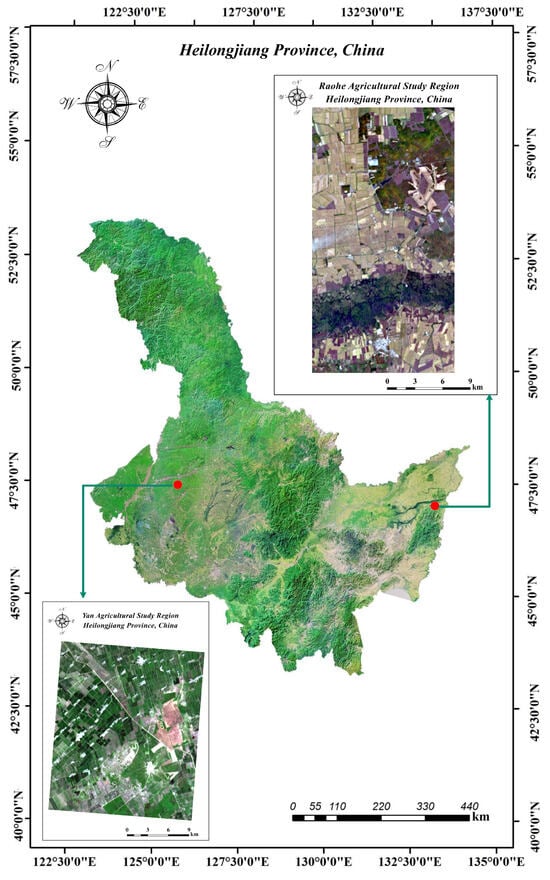
Figure 1.
Study regions of Heilongjiang Province.
- (1)
- A large-scale crop classification dataset has been introduced, named the HLJ dataset. Owing to the diversity of land cover types in agricultural regions, this dataset poses several practical challenges, such as uneven distribution of crops, uncertain crop growth stages, mixed planting, etc., and presents an elevated level of complexity in classification.
- (2)
- This is a large-scale dataset that covers a wide range of rural areas, including a sufficiently representative selection of land cover types in the region. These diverse land-cover types contribute to an exceptionally rich set of spectral information. Furthermore, the proposed dataset contains a sufficient and accurate number of labeled samples, with 319685 and 318942 in the two images, respectively. The reliability of these samples stems from on-site surveys and comprehensive analysis of multitemporal images.
- (3)
- The comprehensive validation of the HLJ dataset was conducted by employing several representative methods for basic classification experiments (e.g., SpectralFormer and SSFTT) and comparing the classification results among different datasets using the same methods. This process affirmed the research value inherent in the issues encompassed by the dataset and its suitability as a benchmark dataset for hyperspectral image classification.
2. Construction of the HLJ Dataset
The HLJ dataset is a satellite-based hyperspectral dataset primarily designed for the classification of large-scale agricultural crops. It was acquired in Heilongjiang Province, located in the northeastern region of China, known for its extensive and concentrated croplands [44]. In this dataset, Raohe County and Yian County in particular have been selected as representatives. They are significant grain-producing regions in Heilongjiang province, providing the most authentic depiction of the agricultural characteristics in this area. Aside from small and concentrated artificial structures, the dataset mainly consists of large-scale cultivated farmlands and natural vegetation.
The two images in the HLJ dataset were acquired using the Advanced Hyperspectral Imager (AHSI) sensor. This sensor finely divides the visible near-infrared (VNIR) spectrum into 76 bands with a spectral resolution of 10 nm. Similarly, the shortwave near-infrared (SWIR) spectrum is segmented into 90 bands, each with a spectral resolution of 20 nm. Given the unique spectral characteristics exhibited by crops at various growth stages, the dataset was captured during the growth and maturity stages, offering a wealth of distinctive spectral information [45,46].
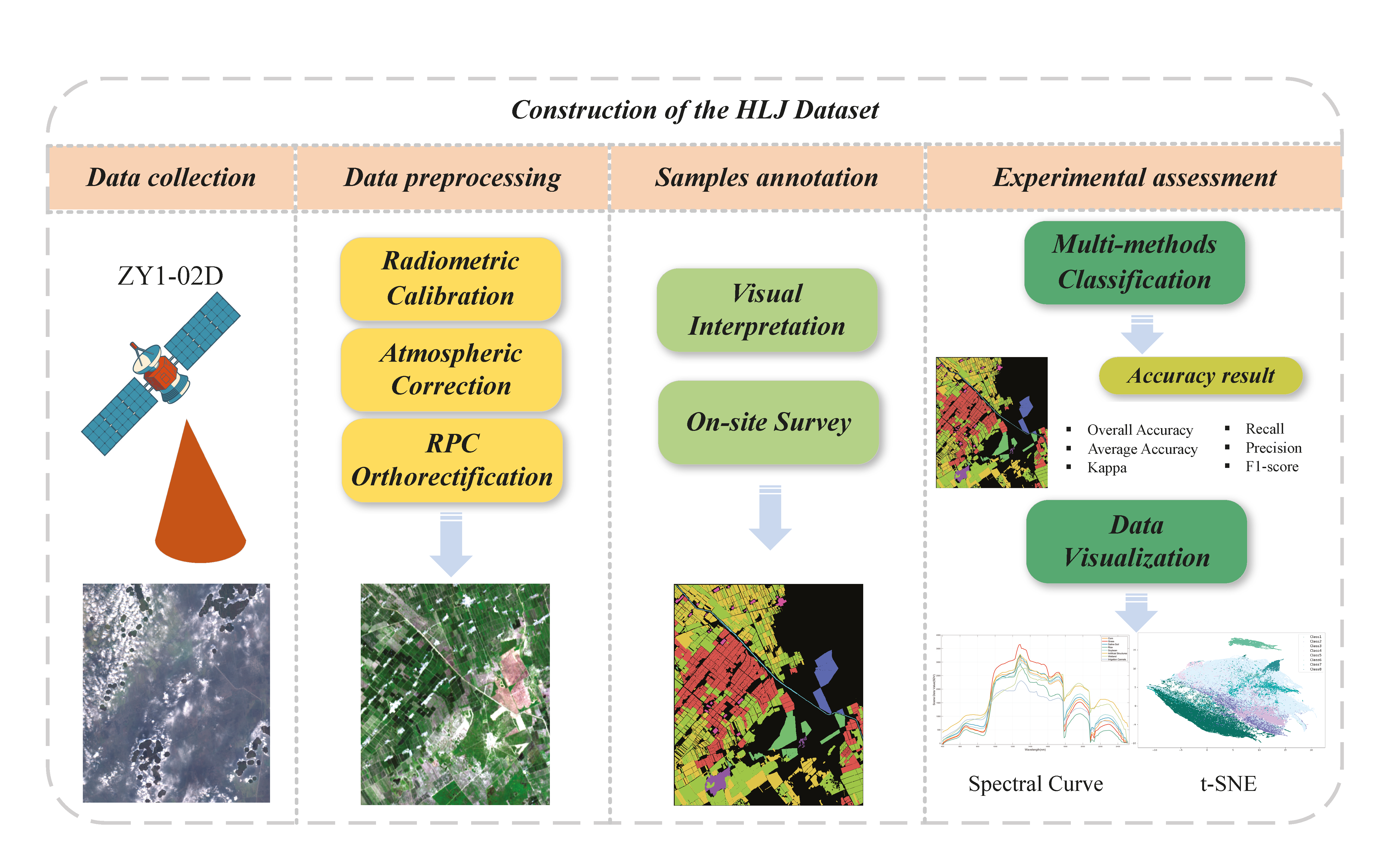
The construction of the HLJ dataset is divided into four main parts as shown in Figure 2: data collection, data preprocessing, sample annotation, and experimental agreement. Section 2.1 presents details about the acquisition of the data. In Section 2.2, details about the preprocessing and the annotation of the proposed dataset are provided. A comprehensive evaluation experiment of the HLJ dataset is introduced in Section 3.
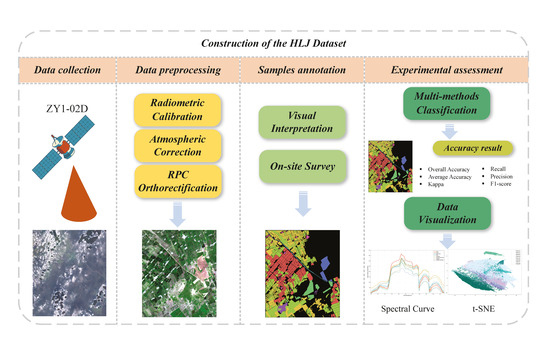
Figure 2.
Flowchart for the construction of the HLJ dataset.
2.1. The Acquisition of HLJ Dataset
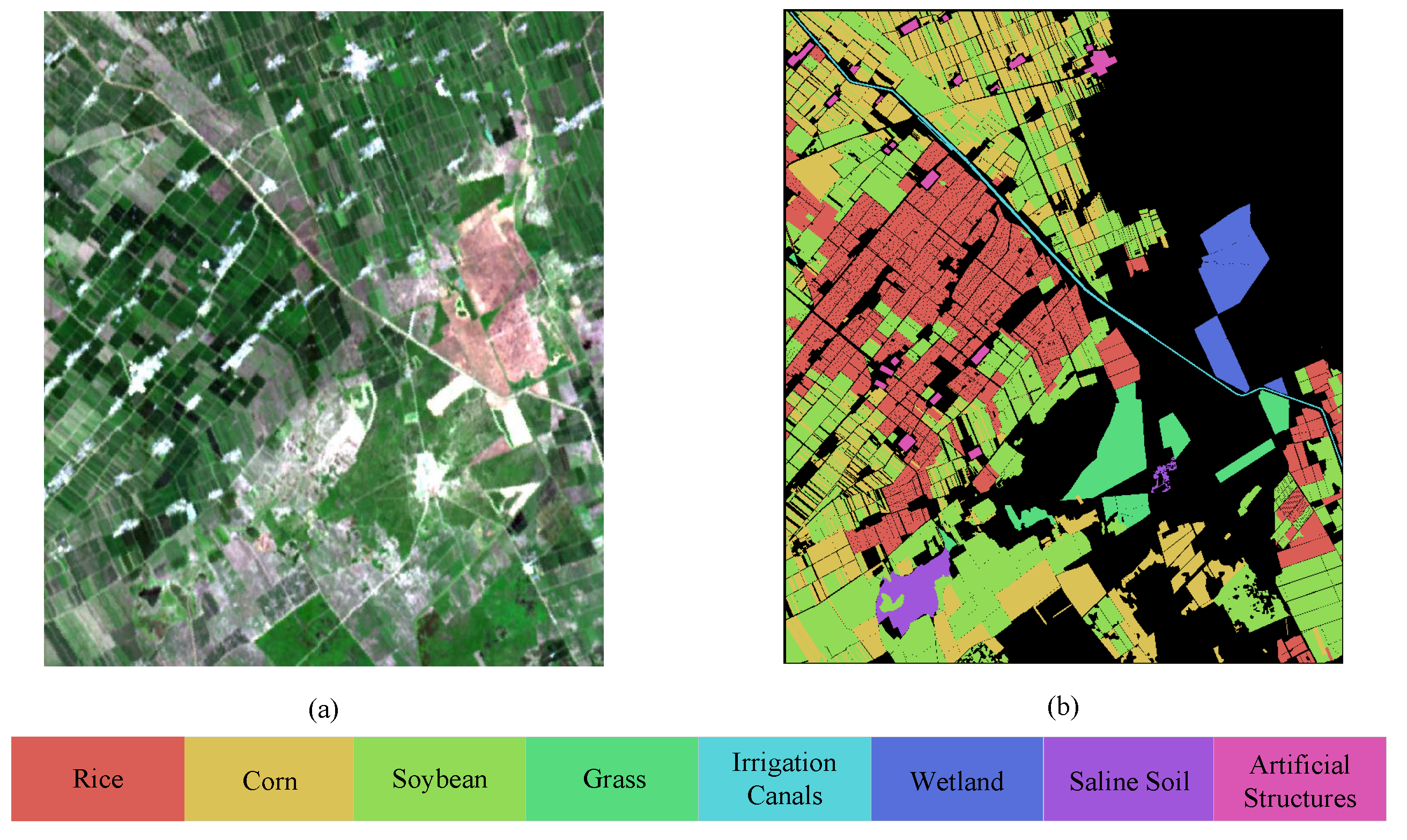
The HLJ-Raohe dataset was captured by the ZY1-02D satellite on 30 September 2022, in Raohe County. Located in the northeastern part of Heilongjiang Province and adjacent to the Ussuri River, Raohe County covers an area of 6765 square kilometers (133°2′N–133°9′N, 47°1′E–47°6′E). The average elevation in this area is 149 m, with a minimum elevation of 45 m and a maximum elevation of 933 m. And the terrain is diverse, including four main types: mountainous hills, plateaus, plains, and wetlands. The dataset was acquired during the maturation stage of the crops, at a time when the crops were not yet harvested, resulting in significant variations in spectral information. The data was captured under favorable weather conditions with good visibility. The image has a size of 897 × 483 pixels and contains 151 spectral bands, covering a wavelength range of 400 to 2500 nm. It is worth noting that the following bands have been removed: Bands 98–102 and 125–132. The HSI acquired by the satellite has a spatial resolution of 30 m. The land cover types are categorized into seven representative classes: Rice, Soybean, Corn, Wetland, River, Built-up land, and Forest. The pseudocolor image and ground truth map are illustrated in Figure 3.
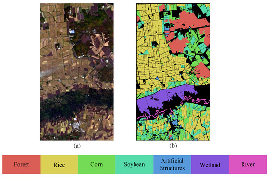
Figure 3.
Pseudocolor image and ground truth map of HLJ-Raohe dataset. (a) Pseudocolor image. (b) Ground truth.
The HLJ-Yan dataset was captured by the ZY1-02D satellite on 10 July 2022, in Yian County. Located in the western part of Heilongjiang Province, Raohe County covers an area of 3678 square kilometers (124°8′N–125°6′N, 47°3′E–47°7′E). The average elevation in this area is 205 m, with a minimum elevation of 154 m and a maximum elevation of 308 m. The primary landforms in this area consist of floodplains, mountainous hills, plains, and wetlands. The dataset was captured during the growth stage of the crops and, at this time, different crops were in varying stages of growth due to differences in planting times. The image has a size of 843 × 719 pixels and contains 149 spectral bands after the removal of broken bands, covering a wavelength range of 400 to 2500 nm. The 17 removed bands include Bands 98–103, 125–133, 165, and 166. The HSI acquired by the satellite has a spatial resolution of 30 m. The land cover types are categorized into eight representative classes: Rice, Soybean, Corn, River, Built-up land, Saline–alkali land, Channel, and Forest. The pseudocolor image and ground truth map of HLJ-Yan are depicted in Figure 4.
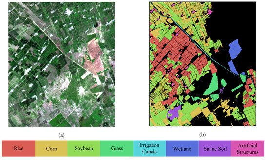
Figure 4.
Pseudocolor image and ground truth map of HLJ-Yan dataset. (a) Pseudocolor image. (b) Ground truth.
2.2. The Data Preprocessing and Annotation Details of the HLJ Dataset
Combining the requirements of the crop structure survey task and the demands of hyperspectral classification methods, the task-specific annotations on two image are conducted. In HLJ-Raohe and HLJ-Yan, 319,685 and 318,942 pixels were labeled, respectively. The category information of HLJ dataset is detailed in Table 1 and Table 2. Combining the requirements of the crop structure survey task and the demands of hyperspectral classification methods, task-specific annotations on the two images are conducted. In HLJ-Raohe and HLJ-Yan, 319,685 and 318,942 pixels were labeled, respectively. Due to the requirement for classification not to be overly detailed in the crop structure survey task, we avoided further subdivision within the same crop. As a result, the number of categories in the dataset may be smaller compared to traditional datasets. Additionally, considering the dataset’s goal of reflecting real planting conditions, we minimized human adjustments to annotated details, especially at the boundaries. Therefore, the distribution of crops in the dataset may be uneven and the number of samples for different categories may be unbalanced. The complete arrangement of the annotation process is as follows: Firstly, five non-professional volunteers participated in the annotation task. They utilized hyperspectral and multispectral images from the same region at different times to perform initial annotations on different but overlapping areas. Subsequently, a comparative analysis of the preliminary annotation results was conducted. For areas with discrepancies and boundary regions, a secondary annotation and discussion were carried out. Additionally, for areas where determination was challenging, three researchers conducted on-site surveys to obtain the final reliable results. In HLJ-Yan, due to dense vegetation in certain image regions causing severe pixel mixing, annotated samples from these areas were excluded. Therefore, the annotation sample proportion has slightly decreased in HLJ-Yan.

Table 1.
The number of labeled samples in the HLJ-Raohe dataset.

Table 2.
The number of labeled samples in the HLJ-Yan dataset.
3. Experimental Settings and Results
This section completes a thorough evaluation to validate the suitability of the proposed dataset as a standard benchmark dataset for HSIC and explores its applicability in a wide range of crop classification. This assessment predominantly involves the performance of mainstream classification algorithms applied to this dataset and comparison across the related datasets. By conducting extensive experiments on this dataset, encompassing a diverse range of classification algorithms that include both traditional machine learning methods and deep learning techniques, the dataset was examined to ascertain its compliance with the prerequisites and objectives of classification tasks. This process aimed to affirm the dataset’s suitability for research purposes and its value within the research community. Meanwhile, as a dataset intended for practical large-scale crop classification tasks, it reveals the obstacles encountered in addressing diversely intricate classification challenges.
All relevant experiments were conducted on hardware with the following specifications: (1) CPU: Intel Xeon Silver 4210R, (2) GPU: Nvidia GeForce RTX 3090, and (3) RAM memory: 32GB. The methods involved in this paper were derived from official open-source projects and were implemented within the official environment.
3.1. Public Datasets
To outline the main differences between the proposed dataset in this paper and existing publicly available datasets, information about several other public datasets is presented. These datasets include WHU-HI-LongKou, WHU-HI-HanChuan, Yellow River Estuary, Salinas, and Indian Pines (https://www.ehu.eus/ccwintco/index.php?title=Hyperspectral_Remote_Sensing_Scenes (accessed on 25 October 2023)).
3.1.1. WHU-Hi Dataset
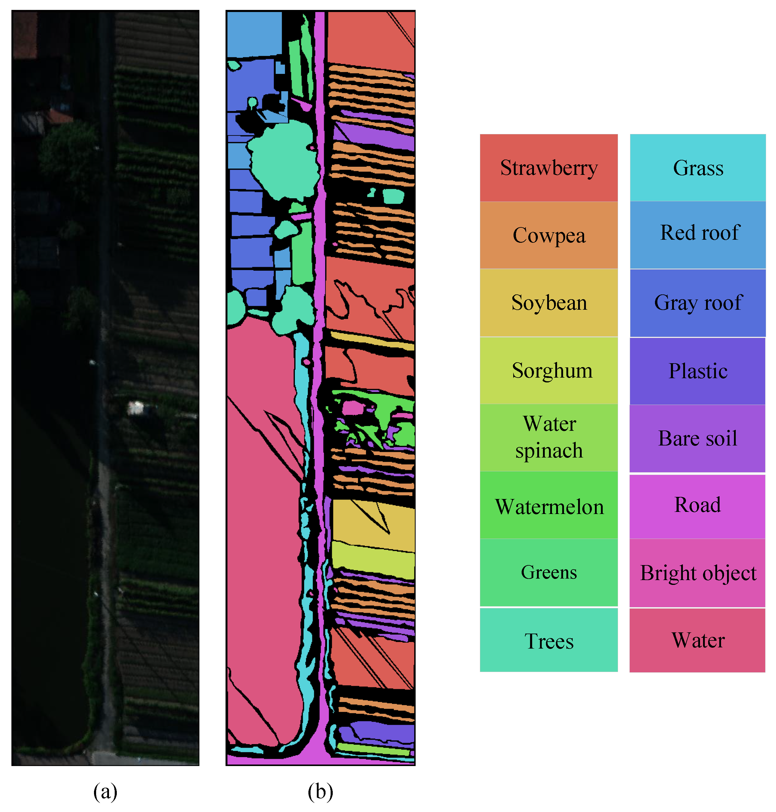
The WHU-Hi dataset is a UAV hyperspectral dataset primarily established for precise crop classification [47]. It is captured in Hubei Province, located in the southern part of China. In contrast to the large-scale agriculture in Heilongjiang Province, the cultivated land is small and fragmented, with numerous villages and human structures. In order to conduct a comprehensive investigation of agricultural cultivation in diverse regions of China, two datasets were employed in this paper: the WHU-Hi-HanChuan dataset and WHU-Hi-LongKou dataset. The pseudocolor image and ground truth map of this dataset are shown in Figure 5 and Figure 6, respectively.

Figure 5.
Pseudocolor image and ground truth map of WHU-Hi-LongKou dataset. (a) Pseudocolor image. (b) Ground truth.
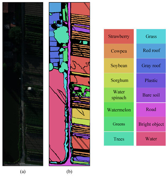
Figure 6.
Pseudocolor image and ground truth map of WHU-Hi-HanChuan dataset. (a) Pseudocolor image. (b) Ground truth.
WHU-Hi-Longkou represents a UAV hyperspectral dataset obtained in Longkou City, located in Hubei Province, China. Captured at a flight altitude of 500 m using the Headwall Nano-Hyperspec imaging sensor, this hyperspectral dataset boasts an impressive spatial resolution of 0.463 m, rendering images with dimensions of 550 × 400 pixels. This dataset encompasses 270 spectral bands that span the wavelength range from 400 to 1000 nm. It includes six distinct crop species. The dataset comprises 128,730 labeled samples, representing nine land cover types.
WHU-Hi-HanChuan is a UAV hyperspectral dataset captured in Hanchuan City, Hubei Province, China. Using a Headwall Nano-Hyperspec imaging sensor, the UAV collected hyperspectral data with dimensions of 1217 × 303 at an altitude of 250 m. The spatial resolution of this image is 0.109 m. This dataset comprises 274 spectral bands covering a wavelength range of 400 to 1000 nm. The dataset captures 255,930 labeled samples and is categorized into 16 land cover types, including 7 distinct crop species.
3.1.2. YRE Dataset
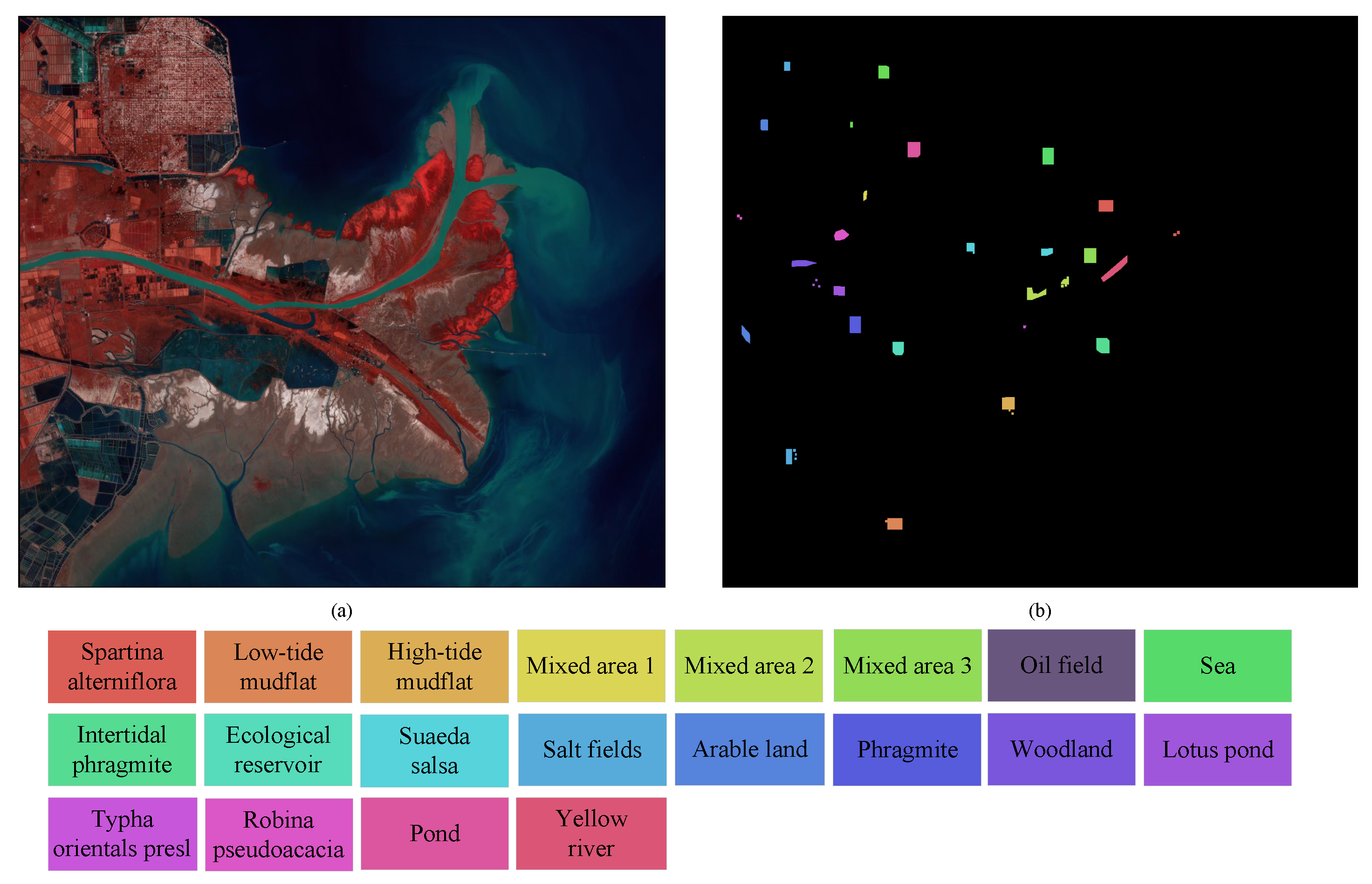
Yellow River Estuary is a satellite-based hyperspectral dataset captured in the Yellow River Delta of Shandong Province [48], China. This is a wetland area located in the northeastern part of Shandong Province. A HSI with dimensions of 1185 × 1342 pixels was captured at the location of the Yellow River Estuary, which covers an area of 2424 × 103 km2 within the delta. The hyperspectral imager on board the GF-5 acquired 150 spectral bands within the VNIR wavelength range (400–1000 nm) at a spectral resolution of 5 nm. In the SWIR wavelength range (1000–2500 nm), it captured 180 spectral bands at a spectral resolution of 10 nm. After removing the broken bands, a total of 285 bands were retained for use in this dataset. This dataset comprises 13,648 labeled samples, representing 20 different wetland land cover types. The pseudocolor image is presented in Figure 7.

Figure 7.
Pseudocolor image and ground truth map of Yellow River Estuary dataset. (a) Pseudocolor image. (b) Ground truth.
3.1.3. Indian Pines Dataset
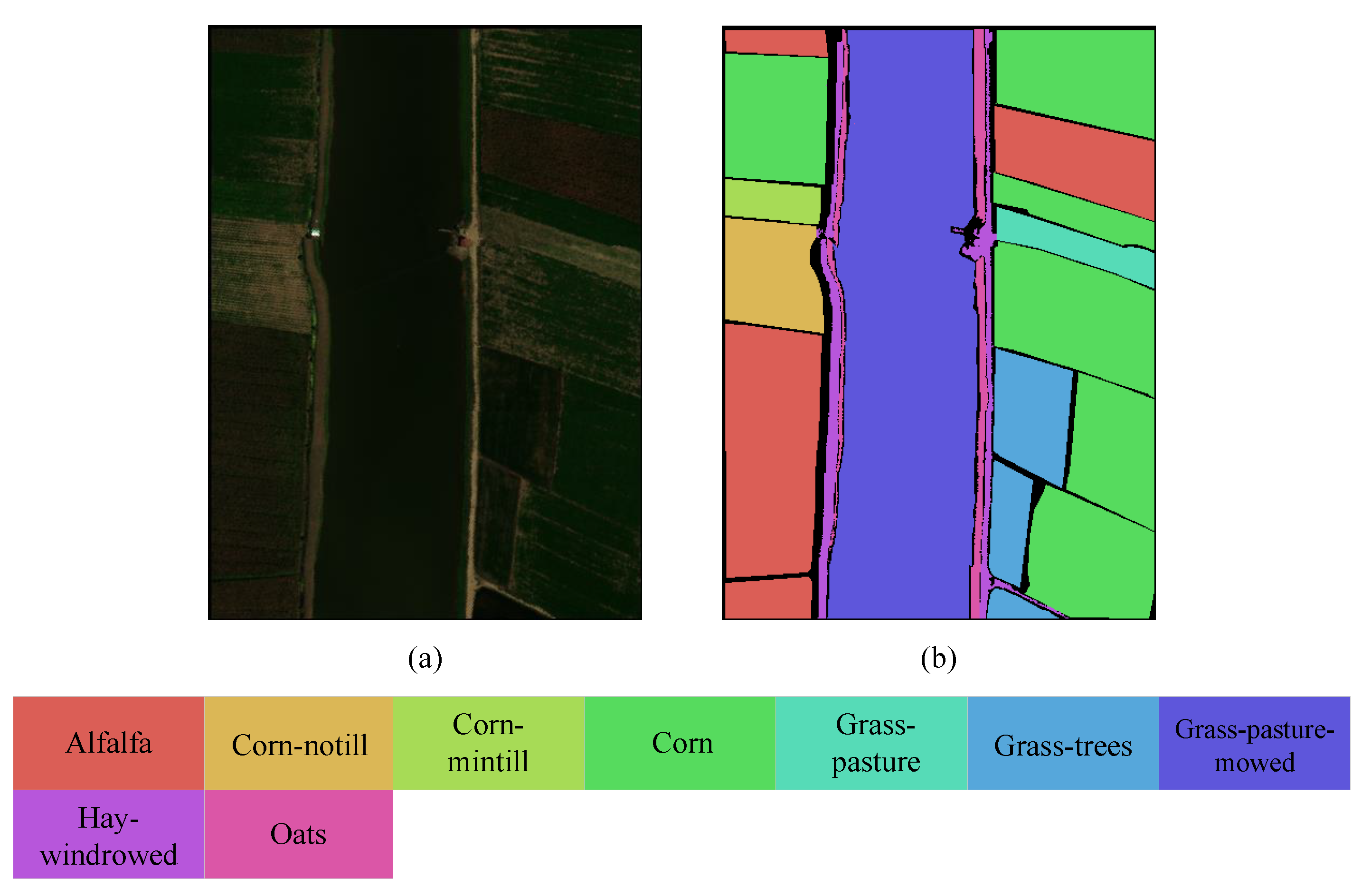
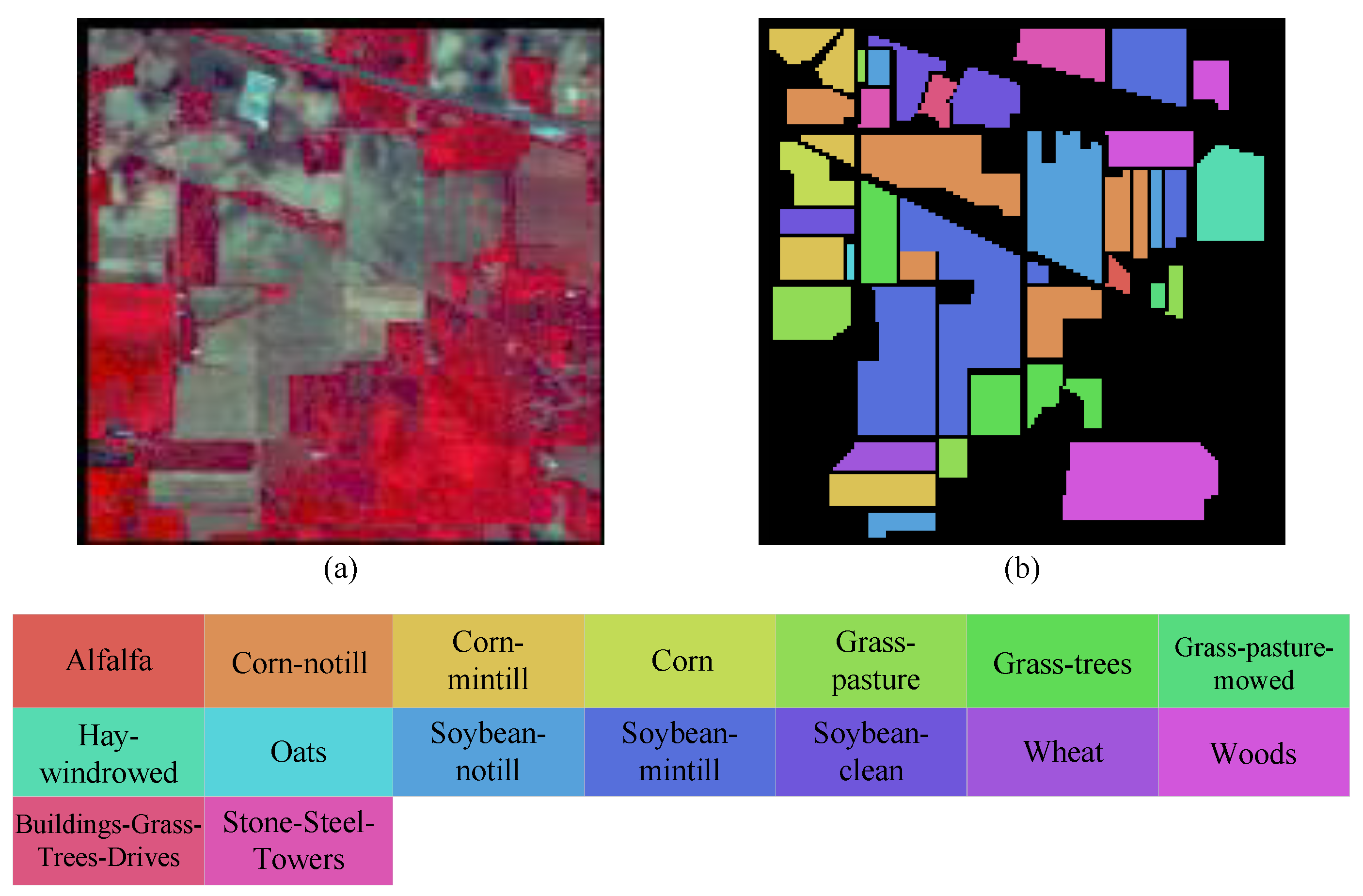
In 1992, the Indian Pines (IP) dataset was captured using airborne visible infrared imaging spectrometer (AVIRIS) sensors over the Purdue University Agronomy farm and its surrounding area in the northwest of West Lafayette, Wisconsin [49]. This is the first hyperspectral image dataset with land cover types focused on natural objects. The imagery was obtained at a spatial resolution of 20 m and has dimensions of 145 × 145 pixels. A total of 16 categories, comprising 10,249 samples, were selected from the image for classification experiments. The spectral information is contained in 200 bands covering the wavelength range from 400 to 2500 nm, with bands affected by water absorption removed. The dataset includes 16 distinct land cover categories. The pseudocolor image and ground truth map is shown in Figure 8.
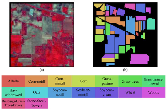
Figure 8.
Pseudocolor image and ground truth map of Indian Pines dataset. (a) Pseudocolor image. (b) Ground truth.
3.1.4. Salinas Dataset
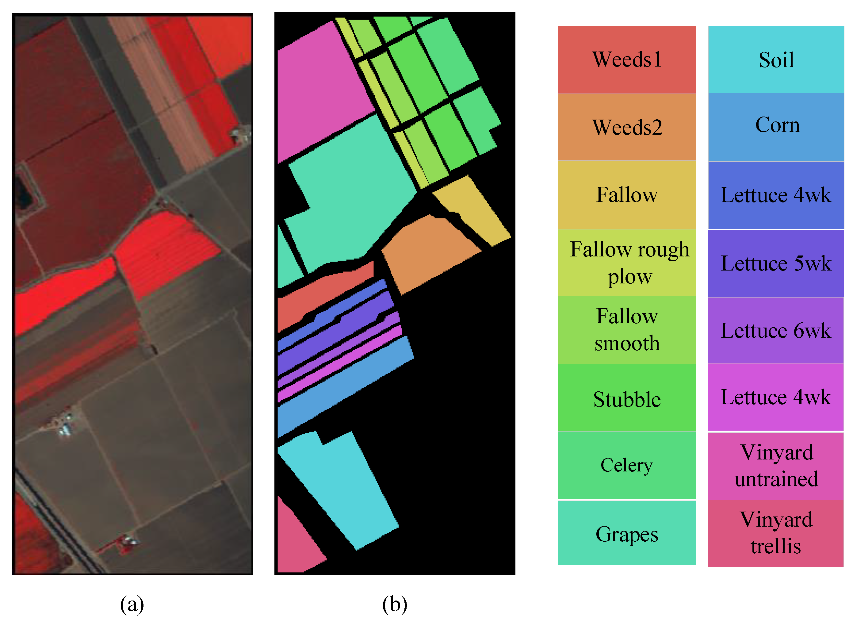
The Salinas dataset was captured in the Salinas Valley region of California, USA in 1998 [50]. It is a hyperspectral image with dimensions of 512 × 217 pixels, featuring a spatial resolution of 3.7 m and a spectral resolution of 10 nm, covering the wavelength range from 400 to 2500 nm. Bands that were affected by water absorption and had low signal-to-noise ratios were removed within this wavelength range, resulting in 204 bands available for classification experiments. The dataset comprises a total of 54,174 labeled samples, categorized into 16 classes. The pseudocolor image and ground truth map is displayed in Figure 9.

Figure 9.
Pseudocolor image and ground truth map of Salinas dataset. (a) Pseudocolor image. (b) Ground truth.
3.2. Classification Experiments of Various Methods on the HLJ Dataset
As a benchmark dataset for HSI classification, its classification effectiveness is the most critical evaluation criterion. Therefore, fundamental classification experiments following the conventional practices were initially conducted. Taking into account the balance between implementation complexity and classification performance, eight representative methods were employed for the classification of this dataset, including the classical classifier SVM, optimized convolutional neural networks, such as the two-dimensional deformable convolutional neural network (2D-Deform), spectral–spatial residual network [51] (SSRN) and dual-branch dual-attention networks [52] (DBDA and DBDA-MISH). Additionally, Vision Transformer [53] (ViT), SpectralFormer [33], and Spectral–Spatial Feature Tokenization Transformer [34] (SSFTT) are representative classification approaches leveraging the transformer structure. The class-specific accuracy (CA), overall accuracy (OA), average accuracy (AA), precision, recall, F1-score (F1) and kappa are considered as the primary evaluation metrics for classification performance.
3.2.1. Experimental Settings
Throughout the implementation of the aforementioned methods, to comprehensively showcase the classification performance of the proposed dataset, this paper adopted the optimal settings in line with the experimental environment. The specific configurations of comparative methods are as follows:
- (a)
- SVM. This serves as the baseline for traditional supervised methods. This method utilizes the machine learning toolkit scikit-learn, maintaining all parameters at their default settings. Using the Radial Basis Function kernel, the penalty parameter C is set to 1.
- (b)
- 2D-Deform. A 2D deformable convolution is chosen as a fundamental convolutional neural network. Stochastic Gradient Descent (SGD) is employed as the optimization approach. The model was trained for 100 epochs with a fixed learning rate of 0.001. After comprehensive consideration of the model parameters, the model’s input is composed of 8 × 8 patches derived from HSI.
- (c)
- SSRN. A modified three-dimensional convolutional neural network with residual connections is used to capture joint spectral and spatial features in the proposed dataset. The method also employs the SGD optimizer with a learning rate of 0.001, trained for 100 epochs. The patch size is 7 × 7.
- (d)
- DBDA. This approach combines attention mechanisms with a convolutional neural network to strengthen the capability of feature extraction and representation through a dual-attention dual-branch structure. This method was trained for 100 epochs, employing a learning rate of 0.001.
- (e)
- DBDA-MISH. In contrast to the DBDA approach, this method incorporates the MISH function as an activation function, aiming to prevent information loss due to the increase in the number of layers in deep neural networks and maintain higher training stability. This method underwent 100 training iterations with a learning rate set at 0.001. Patch size for DBDA and DBDA-MISH is set at 7 × 7.
- (f)
- ViT. This model employs the transformer as the baseline model for image classification. The unique attention mechanism within the transformer allows for capturing global and local features from an overall perspective of the image. For the sake of simplicity in implementation, the ViT method from the open-source project provided in the article is directly utilized. Both the band patch and patch size are set to a default value of 1. The optimizer used is Adaptive Moment Estimation (Adam). The training lasted for 100 epochs.
- (g)
- SpectralFormer. This model focuses on pixel-level HSIC, utilizing the transformer structure for synchronous extraction of spatial–spectral information, rather than employing two separate modules. Distinctive design has enhanced the capability of the transformer-based model to extract local semantic information. Due to memory constraints, this experiment adopts a pixel-wise configuration with a patch size of 1. The band patch is set as 3 to explore the spectral differences among different bands. The model undergoes 100 epochs of training with the Adam optimizer.
- (h)
- SSFTT. This method combines convolutional neural networks and the transformer by utilizing convolutional layers to model low-level spatial–spectral features into tokens. These tokens are then treated as high-level semantic features of HSI, which the transformer excels at handling. In the experiment, PCA is first utilized to reduce the spectral dimensionality to 30. Considering compatibility between the initial and final parts of the model, the patch size is set to 13. The model is trained for 100 epochs.
The majority of the unspecified hyperparameter settings remain consistent with the default configurations mentioned in the reference article, aiming to showcase the fundamental classification performance of the dataset. The results of all experiments were obtained after ten repetitions.
3.2.2. Classification Performance
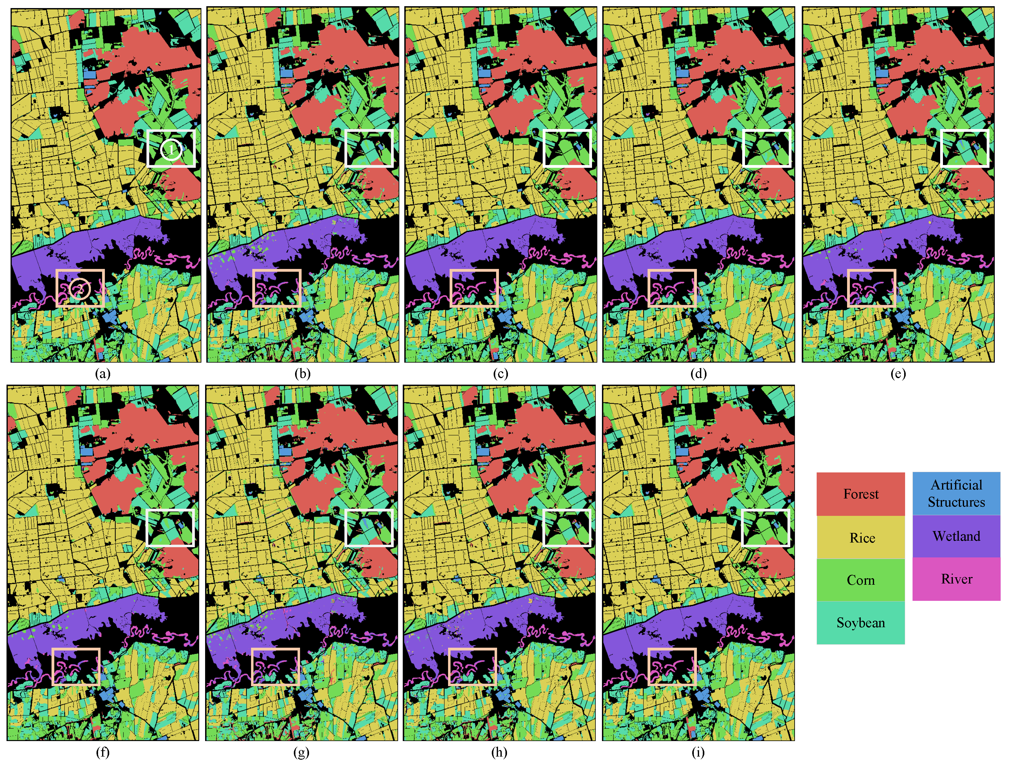
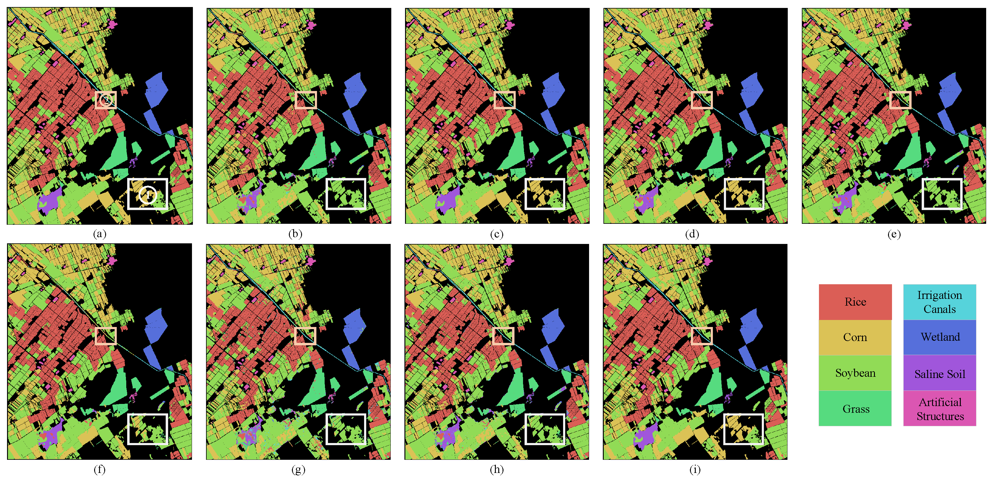
To validate the classification performance of the HLJ dataset, a substantial number of basic classification experiments were conducted. The classification results of different methods are presented in Table 3 and Table 4, and Figure 10 and Figure 11 illustrate the classification maps on the dataset.

Table 3.
Classification results of representative methods on HLJ-Raohe dataset.

Table 4.
Classification results of representative methods on HLJ-Yan dataset.
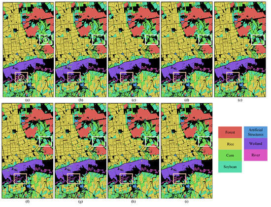
Figure 10.
Classification maps obtained through various methods for HLJ-Raohe dataset. (a) Ground truth, (b) SVM, (c) 2D-Deform, (d) SSRN, (e) DBDA, (f) DBDA-MISH, (g) ViT, (h) SpectralFormer, (i) SSFTT.
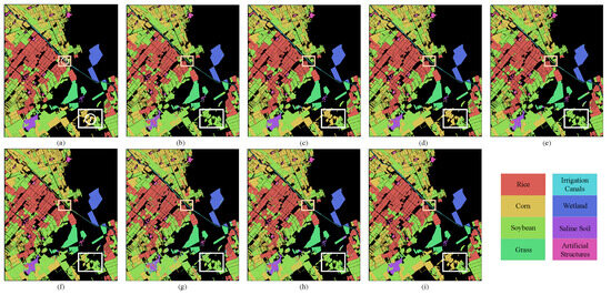
Figure 11.
Classification maps obtained through various methods for HLJ-Yan dataset. (a) Ground truth, (b) SVM, (c) 2D-Deform, (d) SSRN, (e) DBDA, (f) DBDA-MISH, (g) ViT, (h) SpectralFormer, (i) SSFTT.
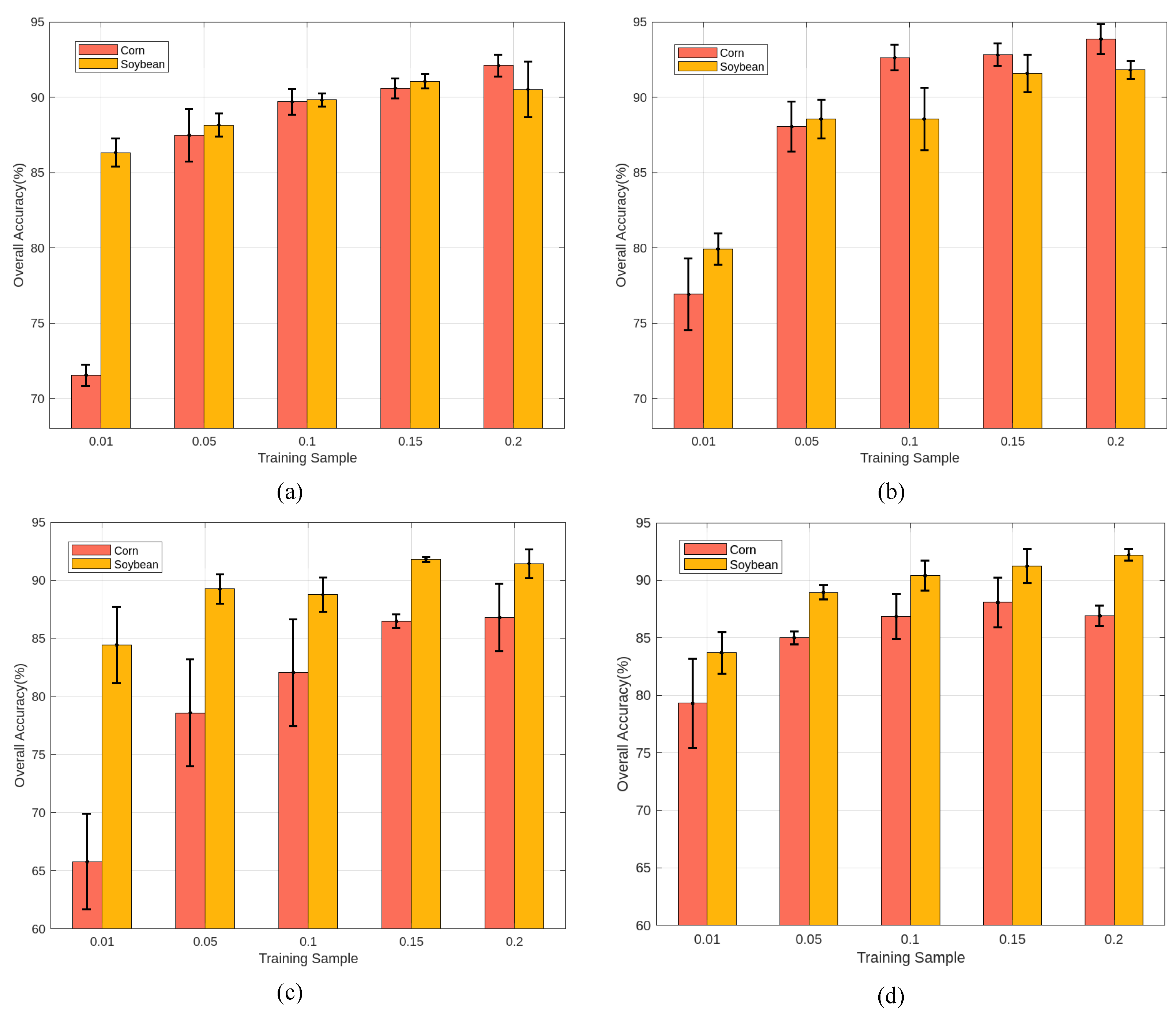
Table 4 shows the classification results achieved by training the HLJ-Raohe dataset with a fixed 10% of samples size per class. With the exception of ViT, the other deep learning approaches have exhibited impressive classification performance; the overall accuracy exceeded 90%. In particular, the SSFTT, SSRN, and 2D-Deform methods accurately classified over 95% of annotated samples; this already represents a significant proportion within a single image. Even with traditional machine learning approaches, SVM showcases robust performance on this dataset. The poor performance of the ViT method might be attributed to the model’s capability to handle single bands, unable to effectively model the extensive continuous spectral information in HSI. However, the HLJ-Raohe dataset is not trivial and holds research significance. Observing the table, it is evident that the classification performance for the third, fourth, and seventh categories is not as ideal as for the other categories. Despite being the best performing methods, SSFTT and 2D-Deform exhibit a clear decrease in accuracy for these specific categories. The observation shown in Figure 10 indicates that the majority of the third and fourth categories were concentrated in complex areas, where these two land cover types are intermingled. It is particularly noticeable in region 1 of the white rectangular box. This means that, in real agricultural scenes, the planting areas for Corn and Soybeans are very close to each other. Additionally, for the River and Wetland categories within the yellow rectangular box region 2, some areas along the riverbank form Wetland during the dry season. But, during the rainy season, these areas are flooded and transform into the river. This seasonal transition results in similar spectral characteristics between the River and the Wetland, posing unknown challenges to the classification models. Figure 12 shows the overall accuracy change in the SSFTT and SSRN for Corn and Soybean categories with variation in training samples. It is noticeable that increasing the number of training samples improves the classification accuracy. However, even with 20% of the training samples, there is no significant improvement.

Figure 12.
The classification performance of Soybean and Corn in different training samples. (a) SSRN method on HLJ-Raohe, (b) SSFTT method on HLJ-Raohe, (c) SSRN method on HLJ-Yan, (d) SSFTT method on HLJ-Yan.
Table 4 presents the experimental results on the HLJ-Yan dataset after training with different methods using 10% of the samples. The SSFTT method achieved the highest accuracy in the classification across all categories. However, it is also worth noting that other classification methods still require substantial improvement on this dataset. This suggests that mainstream methods may encounter certain obstacles in this classification scenario. Similar to HLJ-Raohe, most methods exhibit higher misclassification rates in the Corn and Soybean categories. This can be observed in region 1 of the white rectangular box in Figure 11. This may be attributed to the similar spectral characteristics of Corn and Soybean, as they are both cultivated in dry fields, while Rice, commonly grown in paddy fields, exhibits a significant spectral difference compared to most other cultivated lands. The fifth class is Irrigation Canals; it has an elongated shape and is located among various types of cultivated land. The misclassification areas are mainly concentrated in regions where multiple types of land covers intersect, such as region 2 in the yellow rectangular box. Additionally, due to differences in salt and alkaline content in the soil, Saline Soil from different regions exhibits inconsistent spectral characteristics, which could deceive the model. Even directly increasing the number of training samples as shown in Figure 12 cannot fundamental resolve the mutual interference between Corn and Soybean.
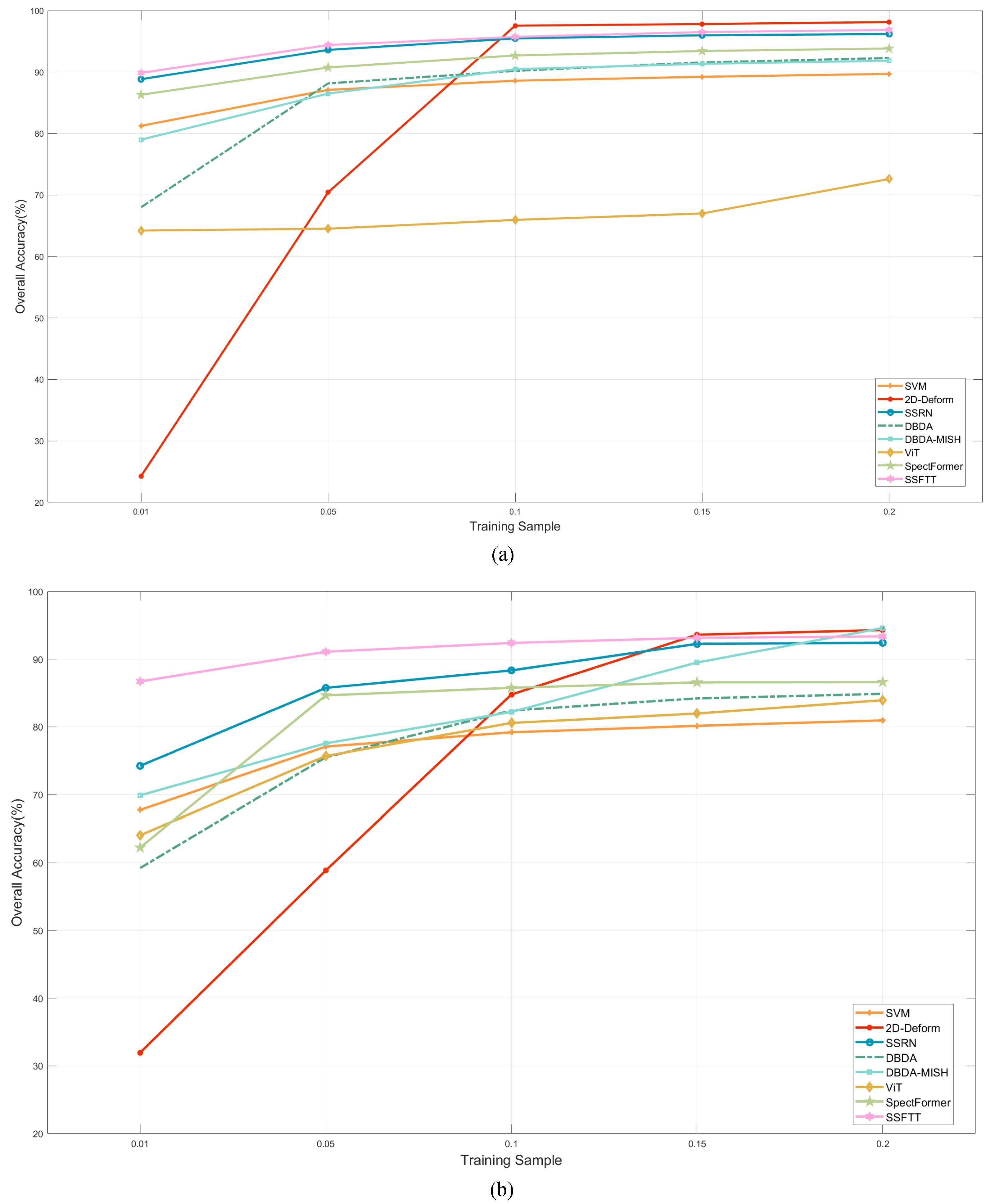
Figure 13 displays the classification results achieved by various methods on the HLJ dataset using different proportions of training samples. As the proportion of training samples increases, the expected rise in OA is observed. However, beyond a training sample size larger than 10%, the improvement in accuracy is quite limited. This indicates that simply applying basic classification methods on the HLJ dataset may not fully capture the crucial information within the data.
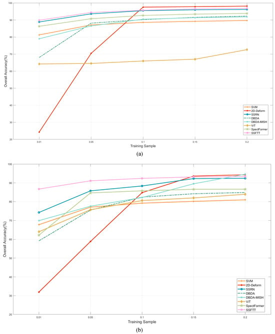
Figure 13.
The classification performance of HLJ dataset with different training samples. (a) HLJ-Raohe, (b) HLJ-Yan.
3.3. Classification Performance on Other Datasets
Table 5 and Table 6 present the classification accuracy of the SSFTT method on other relevant datasets. In order to achieve convergence on them, the training epochs were set to 100. All other hyperparameters were set with the same configuration. With 10% of the training samples, this method exhibited superior performance, exceeding 98% accuracy on various mainstream datasets. Nevertheless, its classification performance experienced a decline when applied to the HLJ dataset. The category with the highest number of labeled samples, Rice, also achieved a classification accuracy of 98%. Furthermore, consistent with the analysis in Section 3.2, severe misclassification occurred for the Corn and Soybean categories in the HLJ-Yan and HLJ-Raohe datasets, posing a significant classification challenge for the entire dataset. Although the classification accuracy of the Oats category in the IP dataset is only 83%, it is important to note that this category has only 20 labeled samples. In the HLJ dataset, no category achieved perfect or complete classification accuracy. Given the substantial number of labeled samples in this dataset, even though the overall classification accuracy for both images reaches 90%, there are still numerous instances of misclassification. Moreover, it is evident that categories with lower classification accuracy require further enhancements in the classification capabilities of the models.

Table 5.
Classification results of the 2D-Deform method on WH-LK, HLJ-Yan, and HLJ-Raohe datasets.

Table 6.
Classification results of the 2D-Deform method on YRE, SA, IP, and WH-HC datasets.
3.4. Visualization of HLJ Dataset
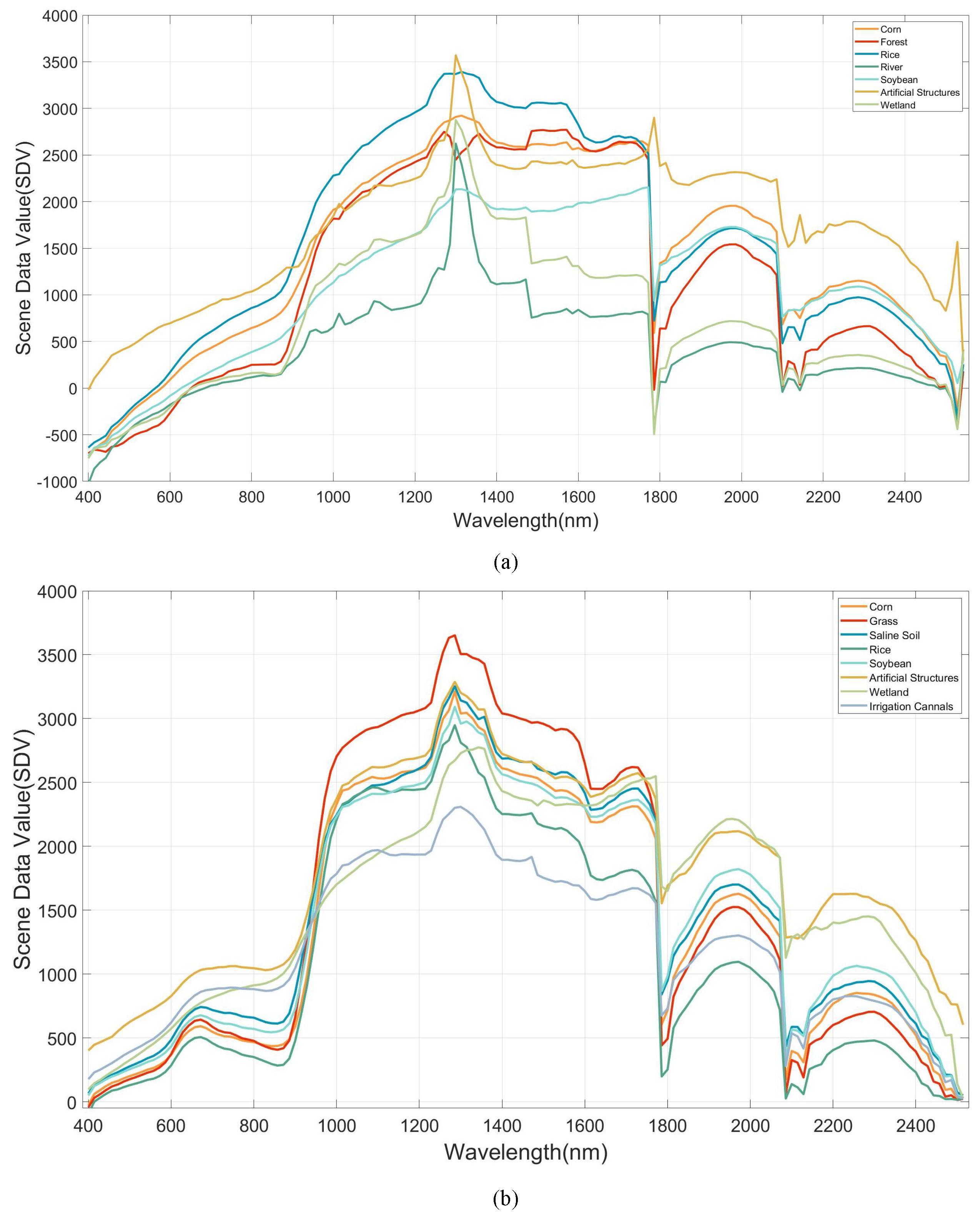
To visually and comprehensively demonstrate the data distribution of the dataset proposed in this paper, 2D visualization of all labeled samples from the HLJ dataset and other datasets was performed using the t-distributed stochastic neighbor embedding (t-SNE) method in this section. The visualization results are shown in Figure 14. Additionally, by computing the average of the image data for all samples, representative spectral curves of different categories in the HLJ dataset were obtained, which can be found in Figure 15.
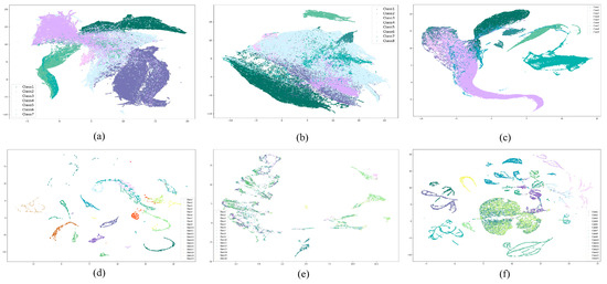
Figure 14.
Visualization of all labeled samples using t-SNE. (a) HLJ-Raohe, (b) HLJ-Yan, (c) WHU-Hi-LongKou, (d) Yellow River Estuary, (e) Indian Pines, (f) Salinas.
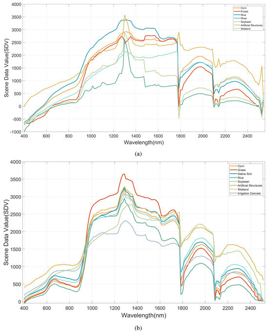
Figure 15.
The spectral curves of HLJ dataset. (a) HLJ-Raohe, (b) HLJ-Yan.
4. Discussion
In this study, a large-scale HSI dataset for crop classification is introduced. By preprocessing the data and meticulous sample annotation efforts, we established two major study areas in Heilongjiang Province, located in northeast China. The images in these areas have large spatial dimensions, covering distinct growth stages of various crops and containing abundant spatial–spectral information. And each image in this dataset provides over 300,000 annotated samples for interpretation. In the fundamental classification experiments, eight classical methods have completed successful classification on the HLJ dataset, which represents the applicability of this dataset as a benchmark dataset. Simultaneously, this dataset also poses practical challenges for many HSIC methods with the characteristics of intensive cultivation and uneven distribution in agricultural scenarios. For instance, as shown in the HLJ-Raohe classification results presented in Figure 10, most methods generate significant misclassifications for Corn and Soybeans. Additionally, categories such as rivers and artificial structures cannot be accurately determined due to their considerably fewer samples compared to other classes. Addressing these challenges requires specific enhancements and modifications to existing hyperspectral classification methods.
The results of the data distribution visualization for the HLJ dataset and other related datasets are presented in Figure 14. In the HLJ dataset, samples within the same category exhibit close proximity, while different categories intertwine. For example, in the HLJ-Raohe dataset, Corn and Soybean display overlap, as well as in the HLJ-Yan dataset. This distribution pattern confirms the suboptimal performance of various classification methods in categorizing these classes in the classification experiments. It is evident that, in the other datasets, there is a substantial dispersion among the sample categories, with small intra-class distances. These datasets are more amenable for modeling due to their characteristics. As shown in Table 5 and Table 6, with the same experimental configuration, the HLJ dataset maintains a higher classification difficulty compared to the other datasets both overall and partially.
The results of the spectral curve visualization for the HLJ dataset are given in Figure 15. Clearly, within specific wavelength ranges, the spectral curves exhibit notable overlap, with similar data values for peaks and troughs. In these bands, models struggle to extract distinctive features, especially in those minute yet crucial segments. This places a higher demand on the model’s ability to maintain precision and sensitivity towards the informative spectral bands.
The HLJ dataset proposed in this study is primarily designed to meet the demands of crop structure investigation in the northeast region. This task only requires accurate classification of major crops such as rice, soybeans, and corn, while maintaining limited focus on other land covers. Constrained by the difficulty of annotation, the labeling process did not involve detailed categorization of more varieties, and different varieties of a single crop were not distinguished. In addition, the impact of more practical factors on hyperspectral interpretation needs further exploration in future research.
5. Conclusions
In this paper, with the purpose of solving the difficulties encountered in crop structure investigation for northeast China, a large-scale HSI benchmark dataset for crop classification is proposed, namely the HLJ dataset. Acquired from the ZY-02D satellite, the dataset reflects the realistic agricultural characteristics of a vast agricultural region, represented by two elaborately selected HSIs. By accurately labeling a total of over 600,000 samples within the entire dataset, including the boundaries of distinct land covers, the limitations of DL in the development of HSIC due to the absence of sample diversity and inadequacy of annotated samples are addressed. And this has been validated through visualizing their features and spectral curves. Additionally, through the basic classification experiments conducted on eight mainstream classification methods, it is found that the mainstream DL methods achieved more than 80% classification accuracy using 10% labeled samples for training. This further confirms the feasibility and research potential of the HLJ dataset as a benchmark dataset for HSI classification. In parallel, compared with the existing traditional datasets, the HLJ dataset faces practical problems such as uneven sample distribution, and intensive and mixed crop cultivation, and their coexistence brings new challenges to the HSIC technique. The HLJ dataset not only serves as a benchmark for measuring the performance of the HSIC algorithm, but is also suitable for serving as a research object for a wide range of practical tasks, such as crop structure survey, long-tailed distribution classification, open-set classification, and so on. In the future, a more in-depth interpretation of this dataset will contribute to enhancing the scientific planning level of agriculture in China, thereby promoting sustainable agriculture and ensuring global food security.
Author Contributions
H.Z. and S.F. were responsible for drafting and editing the initial manuscript; C.Z. conducted the manuscript review; D.W., X.L., and Y.Z. provided the original hyperspectral data and conducted on-site surveys; H.D., S.W., and S.Z. annotated and preprocessed the data. H.Z. and S.F. designed and implemented the relevant experiments. All authors have read and agreed to the published version of the manuscript.
Funding
This work is supported by National Natural Science Foundation of China Grants 62002083 and 62371153, project funded by China Postdoctoral Science Foundation 2023M740265, Open Fund of State Key Laboratory of Remote Sensing Science Grant OFSLRSS202210, Heilongjiang Provincial Natural Science Foundation Grant LH2021F012, the Open Research Fund of Shaanxi Key Laboratory of Optical Remote Sensing and Intelligent Information Processing Grant KF20230401, and Young Elite Scientist Sponsorship Program by Heilongjiang Province 2022QNTJ011.
Institutional Review Board Statement
Not applicable.
Informed Consent Statement
Not applicable.
Data Availability Statement
If you wish to obtain the HLJ dataset, please contact the corresponding author. The data are not publicly available due to the need for further approval from the data owner.
Conflicts of Interest
The authors declare no conflicts of interest.
References
- Wang, S.; Azzari, G.; Lobell, D.B. Crop type mapping without field-level labels: Random forest transfer and unsupervised clustering techniques. Remote Sens. Environ. 2019, 222, 303–317. [Google Scholar] [CrossRef]
- Guerri, M.F.; Distante, C.; Spagnolo, P.; Bougourzi, F.; Taleb-Ahmed, A. Deep Learning Techniques for Hyperspectral Image Analysis in Agriculture: A Review. arXiv 2023, arXiv:2304.13880. [Google Scholar]
- Ozdogan, M. The spatial distribution of crop types from MODIS data: Temporal unmixing using Independent Component Analysis. Remote Sens. Environ. 2010, 114, 1190–1204. [Google Scholar] [CrossRef]
- Liu, J.; Liu, M.; Tian, H.; Zhuang, D.; Zhang, Z.; Zhang, W.; Tang, X.; Deng, X. Spatial and temporal patterns of China’s cropland during 1990–2000: An analysis based on Landsat TM data. Remote Sens. Environ. 2005, 98, 442–456. [Google Scholar] [CrossRef]
- Sethy, P.K.; Pandey, C.; Sahu, Y.K.; Behera, S.K. Hyperspectral imagery applications for precision agriculture—A systemic survey. Multimed. Tools Appl. 2022, 81, 3005–3038. [Google Scholar] [CrossRef]
- Sun, W.; Zhang, L.; Du, B.; Li, W.; Mark Lai, Y. Band Selection Using Improved Sparse Subspace Clustering for Hyperspectral Imagery Classification. IEEE J. Sel. Top. Appl. Earth Obs. Remote Sens. 2015, 8, 2784–2797. [Google Scholar] [CrossRef]
- Gao, F.; Anderson, M.C.; Zhang, X.; Yang, Z.; Alfieri, J.G.; Kustas, W.P.; Mueller, R.; Johnson, D.M.; Prueger, J.H. Toward mapping crop progress at field scales through fusion of Landsat and MODIS imagery. Remote Sens. Environ. 2017, 188, 9–25. [Google Scholar] [CrossRef]
- Debats, S.R.; Luo, D.; Estes, L.D.; Fuchs, T.J.; Caylor, K.K. A generalized computer vision approach to mapping crop fields in heterogeneous agricultural landscapes. Remote Sens. Environ. 2016, 179, 210–221. [Google Scholar] [CrossRef]
- Cai, Y.; Guan, K.; Peng, J.; Wang, S.; Seifert, C.; Wardlow, B.; Li, Z. A high-performance and in-season classification system of field-level crop types using time-series Landsat data and a machine learning approach. Remote Sens. Environ. 2018, 210, 35–47. [Google Scholar] [CrossRef]
- Liu, L.; Xiao, X.; Qin, Y.; Wang, J.; Xu, X.; Hu, Y.; Qiao, Z. Mapping cropping intensity in China using time series Landsat and Sentinel-2 images and Google Earth Engine. Remote Sens. Environ. 2020, 239, 111624. [Google Scholar] [CrossRef]
- Zhang, X.Y.; Yue-Yu, S.; Zhang, X.D.; Kai, M.; Herbert, S. Spatial variability of nutrient properties in black soil of northeast China. Pedosphere 2007, 17, 19–29. [Google Scholar] [CrossRef]
- Shu-hao, T.; Fu-tian, Q.; Heerink, N. Causes and determinants of land fragmentation. China Rural. Surv. 2003, 6, 24–30. [Google Scholar]
- Xiao, L.; Xianjin, H.; Taiyang, Z.; Yuntai, Z.; Yi, L. A review of farmland fragmentation in China. J. Resour. Ecol. 2013, 4, 344–352. [Google Scholar] [CrossRef]
- Yan, S.; Yao, X.; Zhu, D.; Liu, D.; Zhang, L.; Yu, G.; Gao, B.; Yang, J.; Yun, W. Large-scale crop mapping from multi-source optical satellite imageries using machine learning with discrete grids. Int. J. Appl. Earth Obs. Geoinf. 2021, 103, 102485. [Google Scholar] [CrossRef]
- Zhao, C.; Shen, Y.; Su, N.; Yan, Y.; Liu, Y. Gully Erosion Monitoring Based on Semi-Supervised Semantic Segmentation with Boundary-Guided Pseudo-Label Generation Strategy and Adaptive Loss Function. Remote Sens. 2022, 14, 5110. [Google Scholar] [CrossRef]
- Hitouri, S.; Varasano, A.; Mohajane, M.; Ijlil, S.; Essahlaoui, N.; Ali, S.A.; Essahlaoui, A.; Pham, Q.B.; Waleed, M.; Palateerdham, S.K.; et al. Hybrid machine learning approach for gully erosion mapping susceptibility at a watershed scale. ISPRS Int. J.-Geo-Inf. 2022, 11, 401. [Google Scholar] [CrossRef]
- Zhang, C.; Liu, S.; Wu, S.; Jin, S.; Reis, S.; Liu, H.; Gu, B. Rebuilding the linkage between livestock and cropland to mitigate agricultural pollution in China. Resour. Conserv. Recycl. 2019, 144, 65–73. [Google Scholar] [CrossRef]
- Wu, W.; Yu, Q.; You, L.; Chen, K.; Tang, H.; Liu, J. Global cropping intensity gaps: Increasing food production without cropland expansion. Land Use Policy 2018, 76, 515–525. [Google Scholar] [CrossRef]
- Wu, B.; Li, Q. Crop planting and type proportion method for crop acreage estimation of complex agricultural landscapes. Int. J. Appl. Earth Obs. Geoinfor. 2012, 16, 101–112. [Google Scholar] [CrossRef]
- Su, Y.; Gao, L.; Jiang, M.; Plaza, A.; Sun, X.; Zhang, B. NSCKL: Normalized Spectral Clustering with Kernel-Based Learning for Semisupervised Hyperspectral Image Classification. IEEE Trans. Cybern. 2023, 53, 6649–6662. [Google Scholar] [CrossRef]
- Su, Y.; Chen, J.; Gao, L.; Plaza, A.; Jiang, M.; Xu, X.; Sun, X.; Li, P. ACGT-Net: Adaptive Cuckoo Refinement-Based Graph Transfer Network for Hyperspectral Image Classification. IEEE Trans. Geosci. Remote Sens. 2023, 61, 5521314. [Google Scholar] [CrossRef]
- Liu, Q.; Peng, J.; Ning, Y.; Chen, N.; Sun, W.; Du, Q.; Zhou, Y. Refined Prototypical Contrastive Learning for Few-Shot Hyperspectral Image Classification. IEEE Trans. Geosci. Remote Sens. 2023, 61, 5506214. [Google Scholar] [CrossRef]
- Liu, Q.; Peng, J.; Chen, N.; Sun, W.; Ning, Y.; Du, Q. Category-Specific Prototype Self-Refinement Contrastive Learning for Few-Shot Hyperspectral Image Classification. IEEE Trans. Geosci. Remote Sens. 2023, 61, 5524416. [Google Scholar] [CrossRef]
- Rao, N.R.; Garg, P.K.; Ghosh, S.K. Development of an agricultural crops spectral library and classification of crops at cultivar level using hyperspectral data. Precis. Agric. 2007, 8, 173–185. [Google Scholar] [CrossRef]
- Zhang, X.; Sun, Y.; Shang, K.; Zhang, L.; Wang, S. Crop classification based on feature band set construction and object-oriented approach using hyperspectral images. IEEE J. Sel. Top. Appl. Earth Obs. Remote Sens. 2016, 9, 4117–4128. [Google Scholar] [CrossRef]
- Chen, Y.; Jiang, H.; Li, C.; Jia, X.; Ghamisi, P. Deep feature extraction and classification of hyperspectral images based on convolutional neural networks. IEEE Trans. Geosci. Remote Sens. 2016, 54, 6232–6251. [Google Scholar] [CrossRef]
- Li, S.; Song, W.; Fang, L.; Chen, Y.; Ghamisi, P.; Benediktsson, J.A. Deep learning for hyperspectral image classification: An overview. IEEE Trans. Geosci. Remote Sens. 2019, 57, 6690–6709. [Google Scholar] [CrossRef]
- Yu, S.; Jia, S.; Xu, C. Convolutional neural networks for hyperspectral image classification. Neurocomputing 2017, 219, 88–98. [Google Scholar] [CrossRef]
- Huang, Y.; Peng, J.; Sun, W.; Chen, N.; Du, Q.; Ning, Y.; Su, H. Two-Branch Attention Adversarial Domain Adaptation Network for Hyperspectral Image Classification. IEEE Trans. Geosci. Remote Sens. 2022, 60, 5540813. [Google Scholar] [CrossRef]
- Tang, Y.; Feng, S.; Zhao, C.; Fan, Y.; Shi, Q.; Li, W.; Tao, R. An Object Fine-Grained Change Detection Method Based on Frequency Decoupling Interaction for High Resolution Remote Sensing Images. IEEE Trans. Geosci. Remote Sens. 2023, 62, 5600213. [Google Scholar] [CrossRef]
- Feng, S.; Feng, R.; Wu, D.; Zhao, C.; Li, W.; Tao, R. A Coarse-to-Fine Hyperspectral Target Detection Method Based on Low-Rank Tensor Decomposition. IEEE Trans. Geosci. Remote Sens. 2023, 61, 5530413. [Google Scholar] [CrossRef]
- Xi, B.; Li, J.; Li, Y.; Song, R.; Xiao, Y.; Du, Q.; Chanussot, J. Semisupervised cross-scale graph prototypical network for hyperspectral image classification. IEEE Trans. Neural Netw. Learn. Syst. 2022, 34, 9337–9351. [Google Scholar] [CrossRef] [PubMed]
- Hong, D.; Han, Z.; Yao, J.; Gao, L.; Zhang, B.; Plaza, A.; Chanussot, J. SpectralFormer: Rethinking hyperspectral image classification with transformers. IEEE Trans. Geosci. Remote Sens. 2021, 60, 5518615. [Google Scholar] [CrossRef]
- Sun, L.; Zhao, G.; Zheng, Y.; Wu, Z. Spectral–spatial feature tokenization transformer for hyperspectral image classification. IEEE Trans. Geosci. Remote Sens. 2022, 60, 5522214. [Google Scholar] [CrossRef]
- Son, N.T.; Chen, C.F.; Chen, C.R.; Duc, H.N.; Chang, L.Y. A phenology-based classification of time-series MODIS data for rice crop monitoring in Mekong Delta, Vietnam. Remote Sens. 2013, 6, 135–156. [Google Scholar] [CrossRef]
- Tatsumi, K.; Yamashiki, Y.; Torres, M.A.C.; Taipe, C.L.R. Crop classification of upland fields using Random forest of time-series Landsat 7 ETM+ data. Comput. Electron. Agric. 2015, 115, 171–179. [Google Scholar] [CrossRef]
- Zhao, Y.; Feng, D.; Yu, L.; Cheng, Y.; Zhang, M.; Liu, X.; Xu, Y.; Fang, L.; Zhu, Z.; Gong, P. Long-term land cover dynamics (1986–2016) of Northeast China derived from a multi-temporal Landsat archive. Remote Sens. 2019, 11, 599. [Google Scholar] [CrossRef]
- Zhao, C.; Qin, B.; Feng, S.; Zhu, W.; Zhang, L.; Ren, J. An Unsupervised Domain Adaptation Method Towards Multi-Level Features and Decision Boundaries for Cross-Scene Hyperspectral Image Classification. IEEE Trans. Geosci. Remote Sens. 2022, 60, 5546216. [Google Scholar] [CrossRef]
- Zhao, C.; Qin, B.; Feng, S.; Zhu, W.; Sun, W.; Li, W.; Jia, X. Hyperspectral Image Classification with Multi-Attention Transformer and Adaptive Superpixel Segmentation-Based Active Learning. IEEE Trans. Image Process. 2023, 32, 3606–3621. [Google Scholar] [CrossRef]
- Sun, L.; Zhang, J.; Li, J.; Wang, Y.; Zeng, D. SDFC dataset: A large-scale benchmark dataset for hyperspectral image classification. Opt. Quantum Electron. 2023, 55, 173. [Google Scholar] [CrossRef]
- Adão, T.; Hruška, J.; Pádua, L.; Bessa, J.; Peres, E.; Morais, R.; Sousa, J.J. Hyperspectral imaging: A review on UAV-based sensors, data processing and applications for agriculture and forestry. Remote Sens. 2017, 9, 1110. [Google Scholar] [CrossRef]
- Tu, Y.; Bian, M.; Wan, Y.; Fei, T. Tea cultivar classification and biochemical parameter estimation from hyperspectral imagery obtained by UAV. PeerJ 2018, 6, e4858. [Google Scholar] [CrossRef] [PubMed]
- Zhong, Y.; Wang, X.; Xu, Y.; Wang, S.; Jia, T.; Hu, X.; Zhao, J.; Wei, L.; Zhang, L. Mini-UAV-Borne Hyperspectral Remote Sensing: From Observation and Processing to Applications. IEEE Geosci. Remote Sens. Mag. 2018, 6, 46–62. [Google Scholar] [CrossRef]
- Ni, R.; Tian, J.; Li, X.; Yin, D.; Li, J.; Gong, H.; Zhang, J.; Zhu, L.; Wu, D. An enhanced pixel-based phenological feature for accurate paddy rice mapping with Sentinel-2 imagery in Google Earth Engine. ISPRS J. Photogramm. Remote Sens. 2021, 178, 282–296. [Google Scholar] [CrossRef]
- Chong, L.; Liu, H.J.; Qiang, F.; Guan, H.X.; Qiang, Y.; Zhang, X.L.; Kong, F.C. Mapping the fallowed area of paddy fields on Sanjiang Plain of Northeast China to assist water security assessments. J. Integr. Agric. 2020, 19, 1885–1896. [Google Scholar]
- Mao, D.; Wang, Z.; Li, L.; Miao, Z.; Ma, W.; Song, C.; Ren, C.; Jia, M. Soil organic carbon in the Sanjiang Plain of China: Storage, distribution and controlling factors. Biogeosciences 2015, 12, 1635–1645. [Google Scholar] [CrossRef]
- Zhong, Y.; Hu, X.; Luo, C.; Wang, X.; Zhao, J.; Zhang, L. WHU-Hi: UAV-borne hyperspectral with high spatial resolution (H2) benchmark datasets and classifier for precise crop identification based on deep convolutional neural network with CRF. Remote Sens. Environ. 2020, 250, 112012. [Google Scholar] [CrossRef]
- Liu, H.; Li, W.; Xia, X.G.; Zhang, M.; Gao, C.Z.; Tao, R. Central Attention Network for Hyperspectral Imagery Classification. IEEE Trans. Neural Netw. Learn. Syst. 2023, 34, 8989–9003. [Google Scholar] [CrossRef]
- Baumgardner, M.F.; Biehl, L.L.; Landgrebe, D.A. 220 Band AVIRIS Hyperspectral Image Data Set: June 12, 1992 Indian Pine Test Site 3. 2015. Available online: https://purr.purdue.edu/publications/1947/1 (accessed on 20 December 2023).
- Zheng, Z.; Zhong, Y.; Ma, A.; Zhang, L. FPGA: Fast Patch-Free Global Learning Framework for Fully End-to-End Hyperspectral Image Classification. IEEE Trans. Geosci. Remote Sens. 2020, 58, 5612–5626. [Google Scholar] [CrossRef]
- Zhong, Z.; Li, J.; Luo, Z.; Chapman, M. Spectral–spatial residual network for hyperspectral image classification: A 3-D deep learning framework. IEEE Trans. Geosci. Remote Sens. 2017, 56, 847–858. [Google Scholar] [CrossRef]
- Li, R.; Zheng, S.; Duan, C.; Yang, Y.; Wang, X. Classification of hyperspectral image based on double-branch dual-attention mechanism network. Remote Sens. 2020, 12, 582. [Google Scholar] [CrossRef]
- Dosovitskiy, A.; Beyer, L.; Kolesnikov, A.; Weissenborn, D.; Zhai, X.; Unterthiner, T.; Dehghani, M.; Minderer, M.; Heigold, G.; Gelly, S.; et al. An image is worth 16 × 16 words: Transformers for image recognition at scale. arXiv 2020, arXiv:2010.11929. [Google Scholar]
Disclaimer/Publisher’s Note: The statements, opinions and data contained in all publications are solely those of the individual author(s) and contributor(s) and not of MDPI and/or the editor(s). MDPI and/or the editor(s) disclaim responsibility for any injury to people or property resulting from any ideas, methods, instructions or products referred to in the content. |
© 2024 by the authors. Licensee MDPI, Basel, Switzerland. This article is an open access article distributed under the terms and conditions of the Creative Commons Attribution (CC BY) license (https://creativecommons.org/licenses/by/4.0/).


