Article

The ESA Permanent Facility for Altimetry Calibration in Crete: Advanced Services and the Latest Cal/Val Results

1
Geodesy and Geomatics Engineering Laboratory, Technical University of Crete, GR 73100 Chania, Greece
2
European Space Research and Technology Centre (ESTEC), European Space Agency (ESA), Keplerlaan 1, AZ 2201 Noordwijk, The Netherlands
3
Space Geomatica P.C., Xanthoudidou 10A, GR 73132 Chania, Greece
4
European Space Research Institute (ESRIN), European Space Agency (ESA), Largo Galileo Galilei, I 00044 Frascati, Italy
5
Centre National d’Etudes Spatiales (CNES), 31401 Toulouse, France
6
Réseaux et Services en Géodésie Spatiale, Service de Géodésie et de Métrologie, Institut National de L’information Géographique et Forestière (IGN), 94165 Saint-Mande, France
*
Author to whom correspondence should be addressed.
Remote Sens. 2024, 16(2), 223; https://doi.org/10.3390/rs16020223
Submission received: 21 October 2023 / Revised: 2 January 2024 / Accepted: 3 January 2024 / Published: 5 January 2024
(This article belongs to the Special Issue Advances in Satellite Altimetry II)

Abstract

:
Two microwave transponders have been operating in west Crete and Gavdos to calibrate international satellite radar altimeters at the Ku-band. One has been continuously operating for about 8 years at the CDN1 Cal/Val site in the mountains of Crete, and the other at the GVD1 Cal/Val site on Gavdos since 11 October 2021. This ground infrastructure is also supported at present by four sea-surface Cal/Val sites operating, some of them for over 20 years, while two additional such Cal/Val sites are under construction. This ground infrastructure is part of the European Space Agency Permanent Facility for Altimetry Calibration (PFAC), and as of 2015, it has been producing continuously a time series of range biases for Sentinel-3A, Sentinel-3B, Sentinel-6 MF, Jason-2, Jason-3, and CryoSat-2. This work presents a thorough examination of the transponder Cal/Val responses to understand and determine absolute biases for all satellite altimeters overflying this ground infrastructure. The latest calibration results for the Jason-3, Copernicus Sentinel-3A and -3B, Sentinel-6 MF, and CryoSat-2 radar altimeters are described based on four sea-surface and two transponder Cal/Val sites of the PFAC in west Crete, Greece. Absolute biases for Jason-3, Sentinel-6 MF, Sentinel-3A, Sentinel-3B, and CryoSat-2 are close to a few mm, determined using various techniques, infrastructure, and settings.

1. Introduction

Over the past 30 years, satellite altimetry has shown accelerated and continual progress in sensors, measuring technology, new satellites, orbits, and algorithms. Observations from these altimeters are continuously monitoring sea level and climate changes around the globe. They are also used in ocean investigations, coastal oceanography, inland water hydrology, monitoring of Essential Climate Variables (i.e., sea level, sea state, ice sheets, etc.), etc. [1]. To make valuable use of these Earth monitoring signals from altimetry, observations must be accurate, precise, consistent, and uninterrupted over long periods of time.
In this vein, products and services of satellite altimetry need to be verified and validated before they can be put into reliable use for operational oceanography, weather forecasting, and ocean state and climate studies [1]. This verification and validation process spans the entire lifetime of each satellite altimeter before the launch and during its operational phase. After the end of the mission, more often than not, reprocessing of the entire satellite dataset is necessary for long-term and consistent climate data records [2]. Consequently, the quality of these satellite observations needs to be coherently and continuously controlled, but also connected to undisputable reference standards, before the launch and throughout the satellite’s operation.
Satellite altimeters, microwave radiometers, and other onboard instruments are, thus, regularly characterized and calibrated on the ground in special facilities before the launch. After the launch, performance monitoring and calibration take place either on board and/or through dedicated research infrastructures on the ground or in space. These practices make use of natural targets on either the Earth or other celestial bodies, with “specific” signal characteristics (i.e., Moon surface, cold sky), or they employ constructed reference sites on the Earth for calibrating and validating (Cal/Val) the measurements of satellite altimetry.
Over the last 30 years, a few Cal/Val facilities have been developed all over the globe, such as the ERS Venice Tower, Italy [3], the Svalbard [4], the Harvest Oil Platform and Catalina Island, California, USA, operated by the Jet Propulsion Lab, NASA [5], the Ajaccio and Senetosa sites in Corsica, France, maintained by the French space agency (Centre National d’Études Spatiales, CNES) [6], the Bass Strait calibration site in Tasmania, run by the University of Tasmania and the Australian government [7], and the Permanent Facility for Altimeter Calibration of the European Space Agency (ESA) in Gavdos and Crete, Greece [8]. The Permanent Facility for Altimetry Calibration (PFAC) has been providing Calibration/Validation services for all operational satellite altimeters as of 2004. Over the recent years (2020–2023), this ground facility has been expanded and upgraded with new ground reference sites and with the operation of prototype instrumentation for calibration.
Currently, new Cal/Val facilities are being developed in China to calibrate the HY-2 (HY-2A, HY-2B, HY-2C) series of altimeters [9] and the upcoming Guanlan [10], and new sites have also been set up in the USA for the recently launched interferometric altimeter of the Surface Water and Ocean Topography (SWOT) mission [11]. As more space agencies are launching satellite altimeters, more permanent Cal/Val sites are envisaged to operate continuously on a global scale [12].
In 2016 and 2018, respectively, Europe moved into operational altimetry by putting into practice the Copernicus Earth Observation Programme, with the Sentinel-3 A and B, and subsequently, on 21 November 2020 with the Sentinel-6 Michael Freilich (Sentinel-6 MF) satellite. Together with Sentinel-3A/B altimeters [13], and also with CryoSat-2, as well as with SWOT and HY-2 satellites, the Sentinel-6 MF completes a unique constellation for monitoring oceans, inland waters, ice, and climate change [14].
This paper presents the latest (2020–2023) progress made in the PFAC facility, where altimetry calibration is carried out now with two microwave transponders on land and four sea-surface Cal/Val sites on the coasts, placed under satellite orbits. Over the years, this PFAC facility has built the capacity to perform the following functions:
(a)
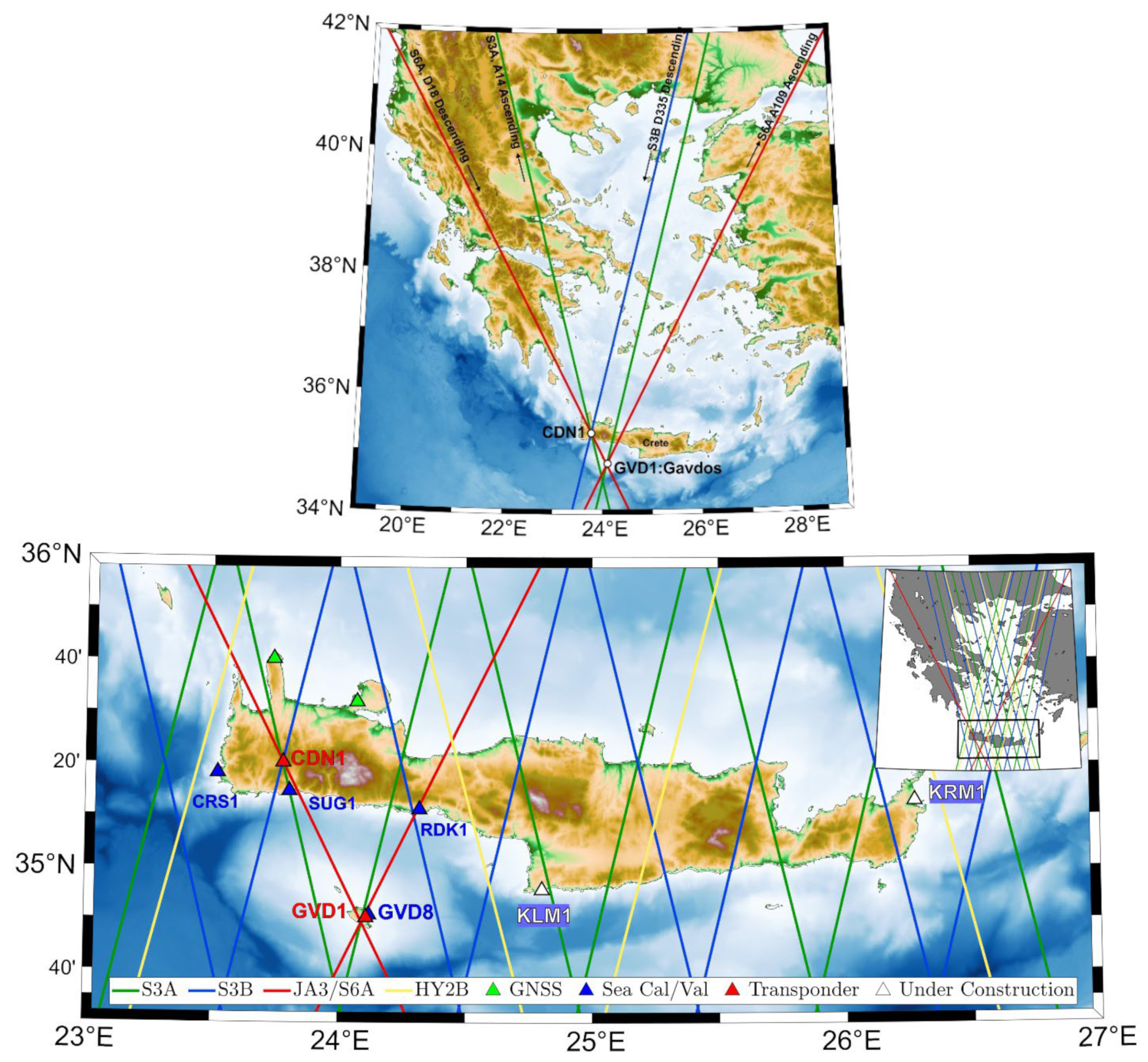
To provide Cal/Val services for all international satellite altimeters, such as Sentinel-6 MF, Sentinel-3A, Sentinel-3B, CryoSat-2, HY-2A, HΥ-2B, HY-2C, the Jason series, SARAL/AltiKa, and Envisat (Figure 1) (Multi-satellite capacity).
(b)
To integrate various Cal/Val inputs coming from a combination of different reference sites, observations, settings, and technologies, and, thus, to monitor the performance of a satellite altimeter reliably, and resolve relationships among different missions (Integration and Synthesis capacity).
(c)
To operate this PFAC infrastructure in conformity with the Fiducial Reference Measurements (FRM) recommendations. The facility, thus, supports calibration with redundant ground instrumentation, operating in diverse settings (mountains, coasts, different altitudes, orbit crossovers, etc.), of different types (e.g., GPS, GLONASS, Galileo, DORIS, sea-surface, transponders, etc.), various instrument makes, with distinct measuring technologies (e.g., acoustic, pressure, radar tide gauges, etc.), and instrumentation situated at reference sites where Cal/Val results could be cross-examined, validated, and, thus, ensured (Diverse Reference capacity).
(d)
To report measures for describing uncertainty for the Cal/Val results [15], following the strategy of FRM, prescribed by the ESA. As such, it evaluates the quality of satellite altimetry products in a standardized, consistent way and with confidence [16,17] (FRM Uncertainty Reporting capacity).
(e)
To adapt to future challenges of calibration solicited by the new wide swath [18], interferometric, and Ka-band altimetry [19] (Adaptation capacity).
(f)
To augment its reference baseline for calibrating other parameters of altimetry (e.g., backscatter coefficient, spacecraft orientation in space, sea state and wind [20]) and for implementing alternative techniques of calibration with GNSS interferometric reflectometry [21,22], corner reflectors [23], microwave radiometers [24], etc. (Multiple Parameter Calibration capacity).
The current PFAC status, after the upgrade and modernization of its infrastructure and instrumentation, is presented in Section 2. The dataset of the ground measurements and satellite products used and the procedures followed to monitor their FRM quality are given in Section 3. The latest absolute and relative Cal/Val results for Sentinel-6 MF, Sentinel-3A/B, CryoSat-2, and Jason-3 missions are given in Section 4, along with the intercomparison of results as derived by diverse techniques (i.e., transponder versus sea-surface) and different settings (i.e., the CDN1 transponder in the Crete high mountains versus the GVD1 transponder on low-elevation Gavdos Island, the sea-surface Cal/Val in Gavdos versus the Crete results with its SUG1 and RDK1 sites). Finally, Section 5 provides the conclusions of this work with a special focus on the performance of the Sentinel-6 MF Poseidon-4 altimeter during its Commissioning and Tandem phases with Jason-3, but also with respect to Sentinel-3A/B Synthetic Aperture Radar altimeters.

2. The PFAC Infrastructure and Instrumentation Modernization

Two transponder (CDN1 and GVD1) and four sea-surface (Gavdos, RDK1, CRS1, SUG1) Cal/Val sites comprise the monitoring reference stations of the PFAC (Figure 1), at this point in time. A network of continuously operating GNSS stations and an Operations Control Center support the operations and services provided by the PFAC. A detailed description of the PFAC infrastructure and instrumentation was presented in 2020 [15]. Since then, two more permanent stations have been established and are currently operational: the GVD1 transponder site on Gavdos Island and the SUG1 sea-surface Cal/Val site in southwest Crete. A description of both follows.

2.1. The GVD1 Transponder Cal/Val in Gavdos

2.1.1. Justification for Another Transponder

The first CDN1 Ku-band range transponder in the mountains of west Crete has been continuously operational since 2015. This CDN1 transponder acts as a stable point target of reference on land and advances our capacity to reliably monitor the altimeter’s main observation, that of range. A transponder provides a single-point impulse response rather than a response from the averaging of different reflection points at sea, as is done in sea-surface calibrations (Figure 2). Although this site is ideal in terms of signal quality and clear target identification, weather conditions over winter are harsh (snow, heavy rain, thunderstorms, and lightning) and at times calibrations cannot be performed due to prevailing conditions (Figure 3). Cancellations of CDN1 transponder calibrations may occur particularly over January and February each year because of bad weather, although the cancellation rate appears to be relatively small (~8%) and a sufficient timeline is maintained.
Despite that performance, there was no other transponder available at that time to provide a cross-examination for its observations, but also to act as a backup in case of failure of the CDN1 transponder. To decrease the consequences of a component failure of the CDN1 transponder, be it, for example, antenna or electronics, a redundant configuration was planned.
A set of redundant transponders would support continuous calibrations and protect us from irreversible calibrations and extended restart times in case of failure. Thus, to eliminate dependence on a single transponder, while at the same time providing alternatives and redundant observations for the altimetric range from a different setting and perspective, it was decided to set up another transponder on the island of Gavdos. This site has been called the GVD1 transponder Cal/Val site.
Gavdos Island was selected to host the new transponder because of the following factors:
(1)
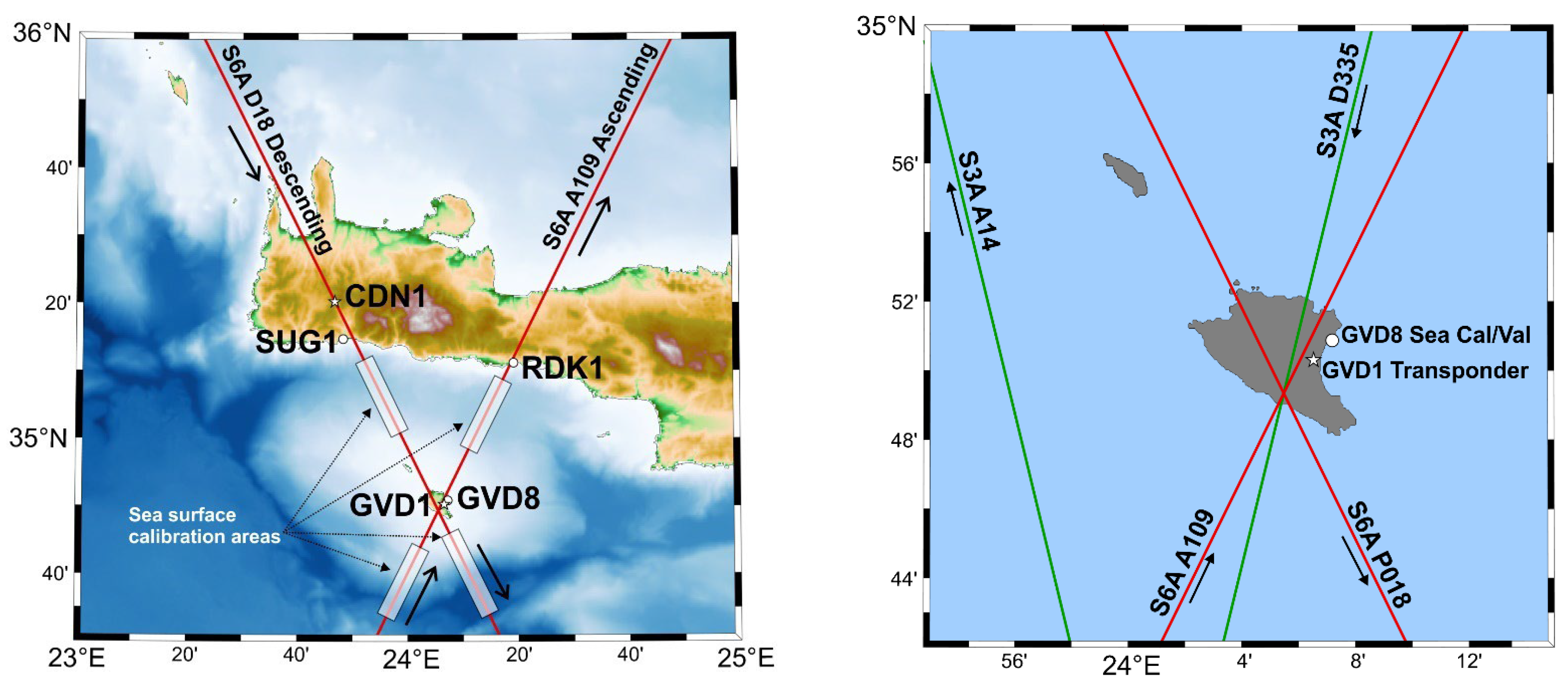
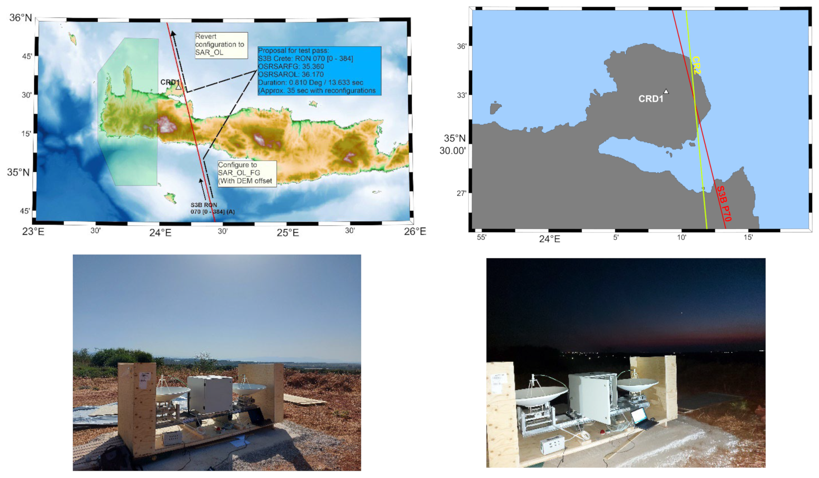
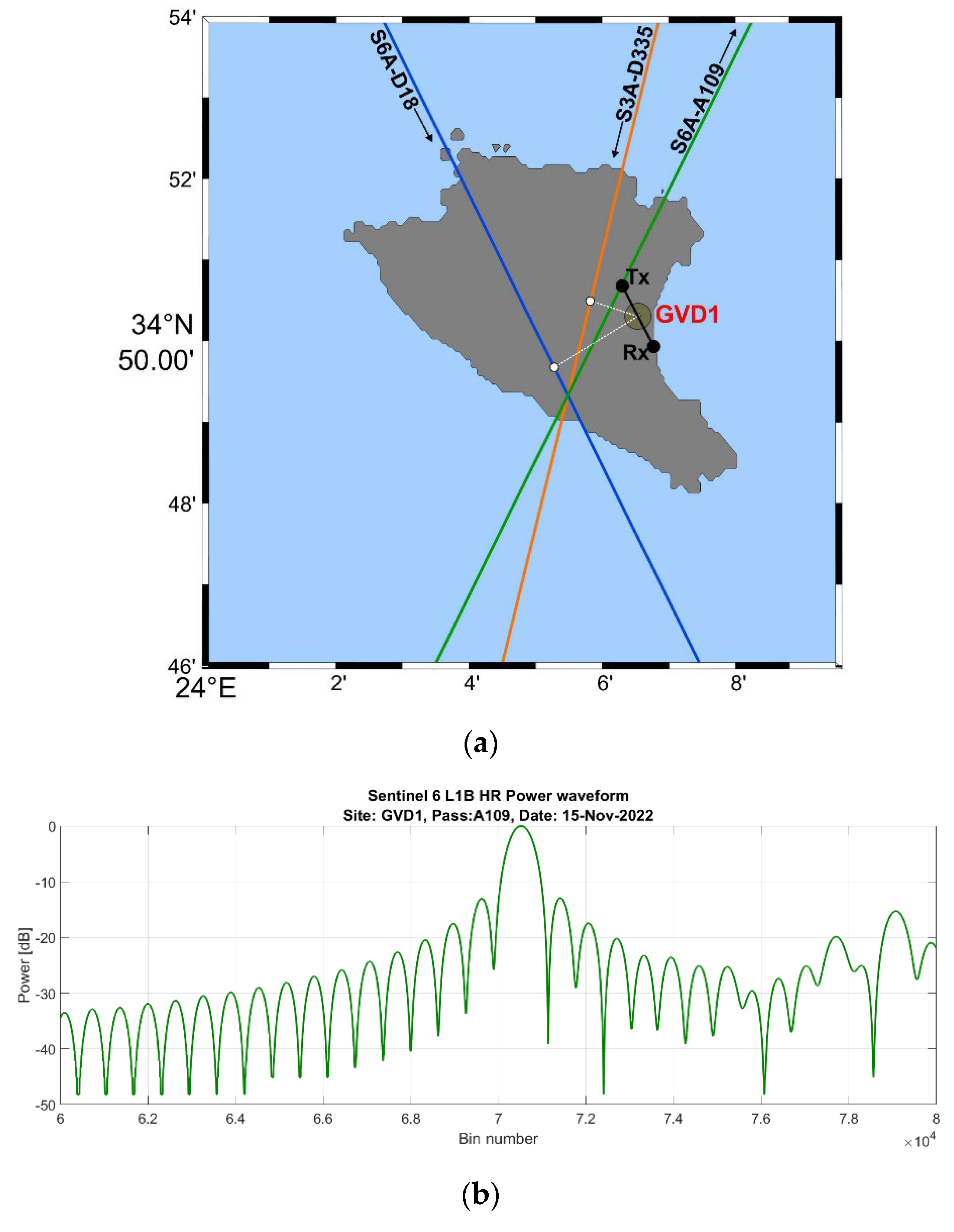
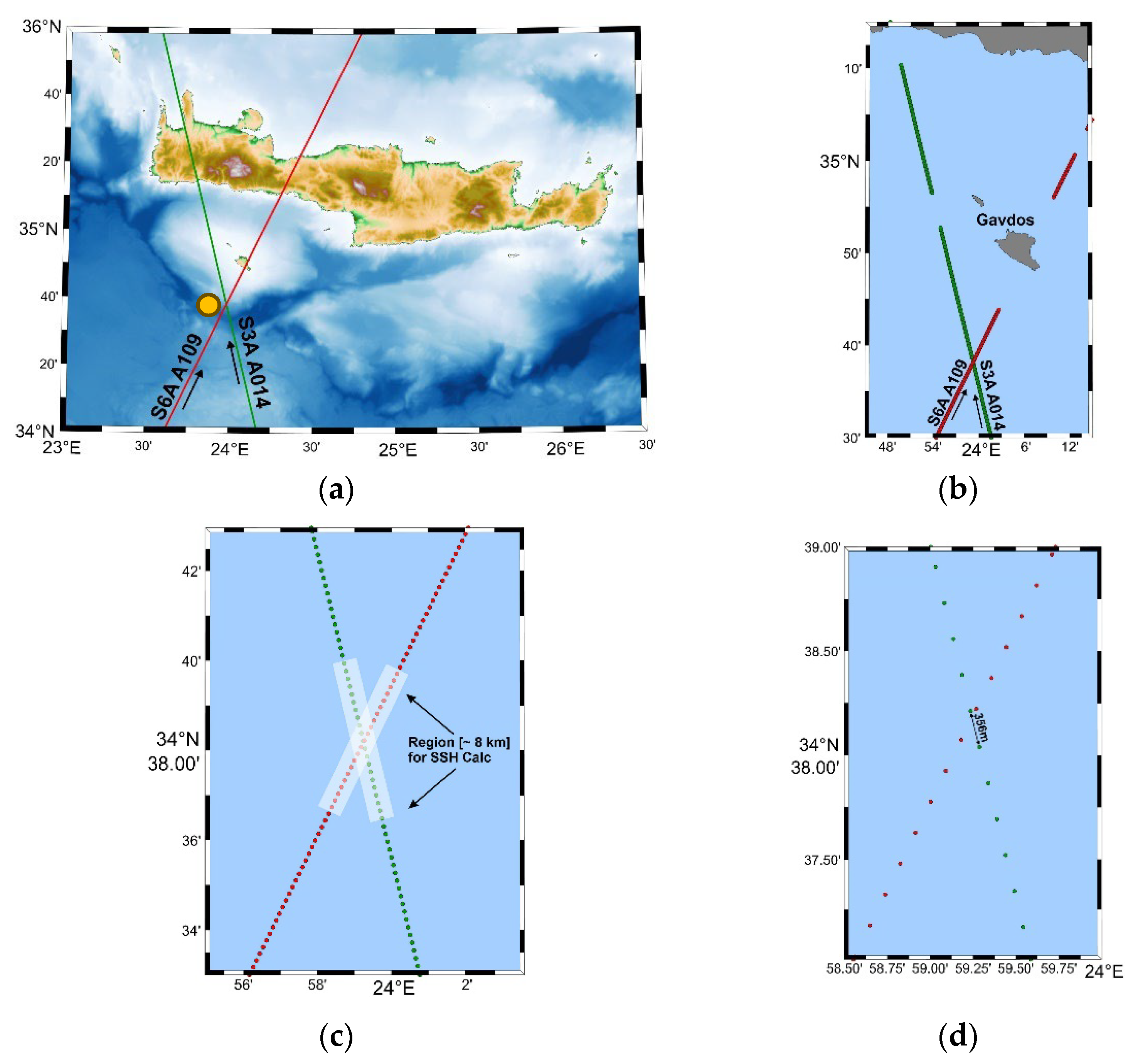
The chosen GVD1 site lies, for the first time, under a triple crossover of the ground tracks for the descending (D18) and ascending (A109) pass of Sentinel-6 MF and also for the descending Pass D335 of Sentinel-3A (Figure 4). Hence, satellite ground track and related directional angle errors can, in principle, be established;
(2)
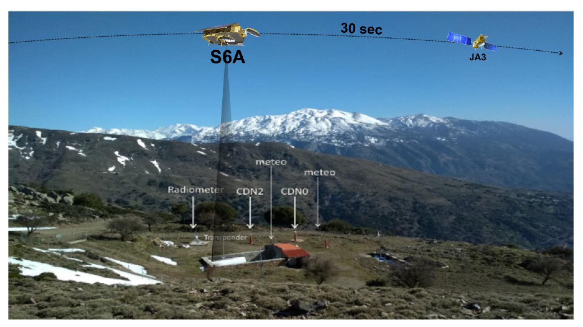
The GVD1 site is separated, along the same descending orbit D18, by only 9 s from the CDN1 transponder in the mountains of Crete. Thus, Sentinel-6 MF observations are monitored almost simultaneously with the instrumentation of different technology and with diverse conditions and settings;
(3)
The new site in Gavdos presents the advantage of tying transponder observations to the major sea-surface Cal/Val site, only 2 km away, on Gavdos Island, which has been operating for almost 20 years;
(4)
Measuring conditions of the GVD1 transponder are quite different from the transponder in the mountains. GVD1 is located at a lower elevation (about 98 m above sea level) than the CDN1 transponder and operates with totally different atmospheric conditions and different technology. Accordingly, transponder results could be objectively controlled;
(5)
The establishment and operation of a transponder at GVD1 at a crossover location doubles the number of transponder calibrations for Sentinel-6 MF. For example, it monitors the satellite every 4 and 6 days consecutively, instead of every 10 days (precisely, every 9 days and 22 h) [25], as is commonly done at CDN1 with a descending orbit D18 alone;
(6)
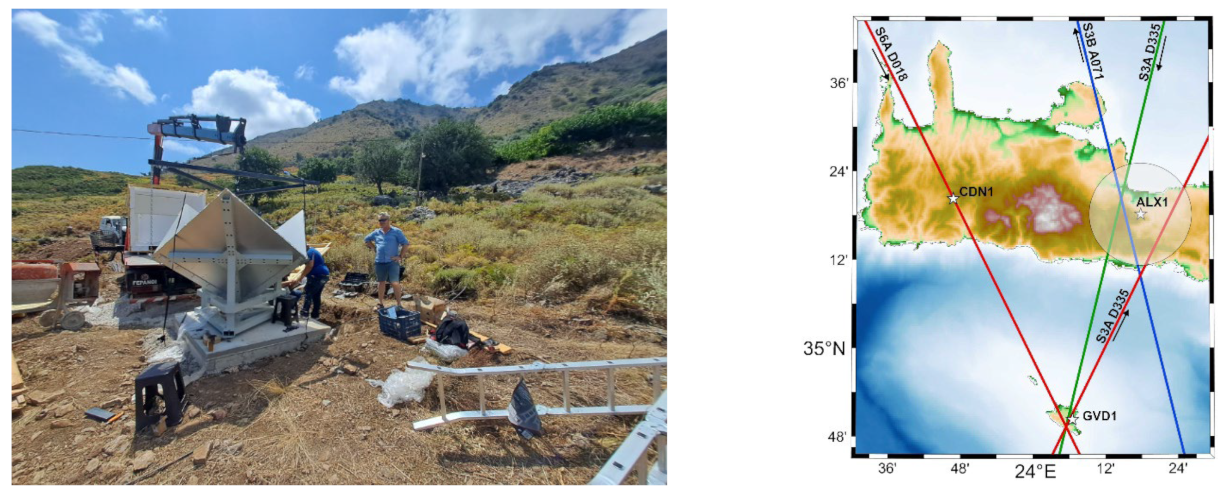
The establishment of this GVD1 transponder supports the goals of the FRM strategic plan for monitoring satellite altimetry. This is because the performance of the Sentinel-6 MF is evaluated along the same descending pass (D18) by two sea-surface (GVD8 in Gavdos and SUG1 in Crete) and two transponder (CDN1: west Crete and GVD1: Gavdos) Cal/Val facilities (Figure 5). This one-of-a-kind geometry ensures the required redundancy for monitoring Sentinel-6 MF with this ground facility in Gavdos and Crete.
Finally, the relative calibration of Sentinel-6 MF against Sentinel-3A, as performed with the GVD1 transponder, uniquely satisfies the consistency requirements of satellite altimetry observations towards mesoscale oceanography (Figure 1, Figure 4, and Figure 5).

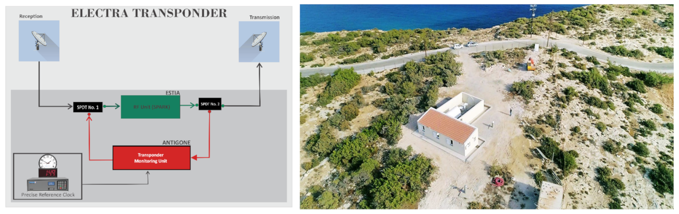
2.1.2. The New “ELECTRA” Transponder in Gavdos

The new transponder instrument installed in Gavdos is called “ELECTRA”. Its design, manufacturing, characterization, testing, and installation took place in the period February 2020–October 2022. This transponder is not a replica of the existing CDN1 transponder. It was developed anew based on the experience gained from the older CDN1 transponder with some novel characteristics, such as the following:
  • Dual operation for range and sigma-naught calibration. The ELECTRA transponder was designed to support absolute calibration, not only for the range, but also for the backscatter coefficient (sigma-naught). This combined technology emerged, for the first time, to simultaneously calibrate range and sigma-naught in satellite altimetry.
  • The motivation for a double and simultaneous calibration in Gavdos was related to the ability, in the first place, to secure and strengthen the operational capabilities of the range calibration at the CDN1 transponder in Crete, and further to bolster the recently refurbished ESA sigma-naught transponder in Italy [26].
  • Selectable gain. The electronics of the ELECTRA transponder can be selected to amplify, when required, the received signal by 1-dB steps and in the range between 75 dB and 80 dB. This function permits transponder operations for several satellite altimeters with differing altitudes and signal strengths.
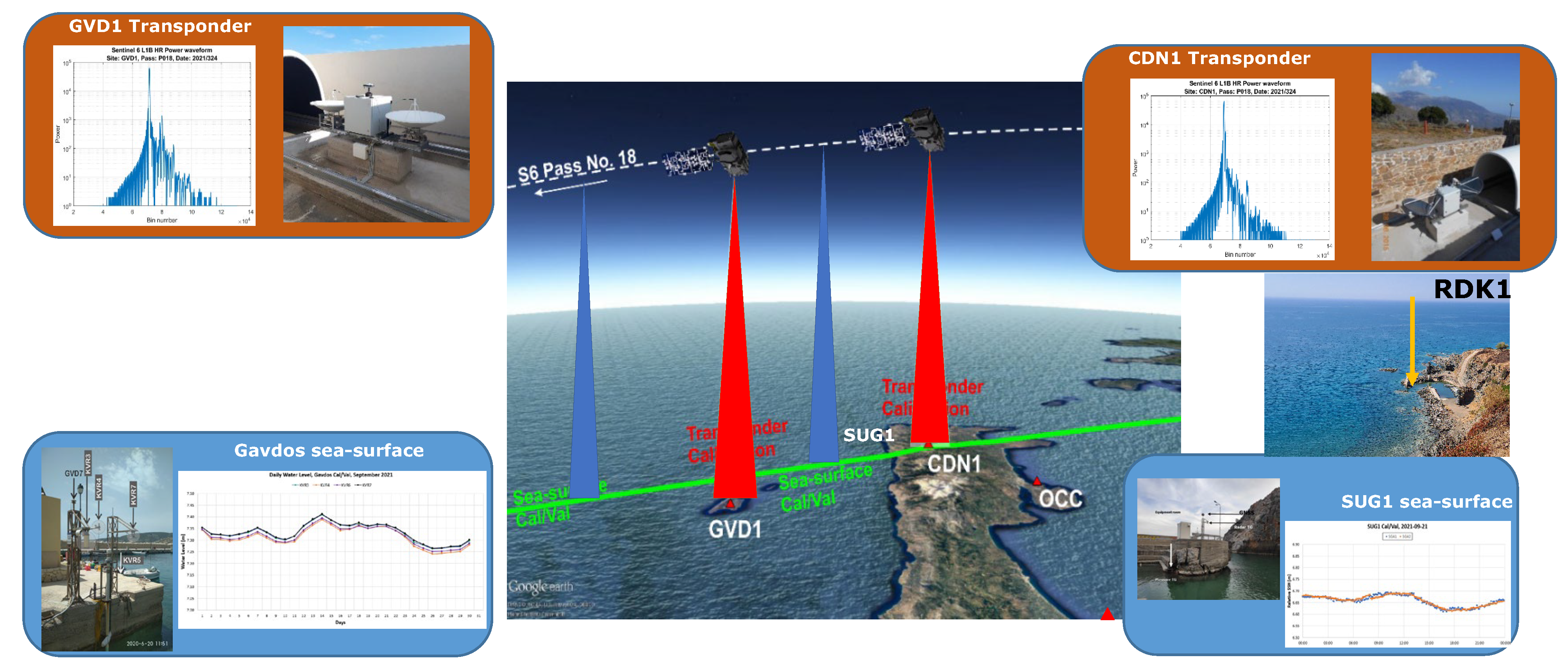
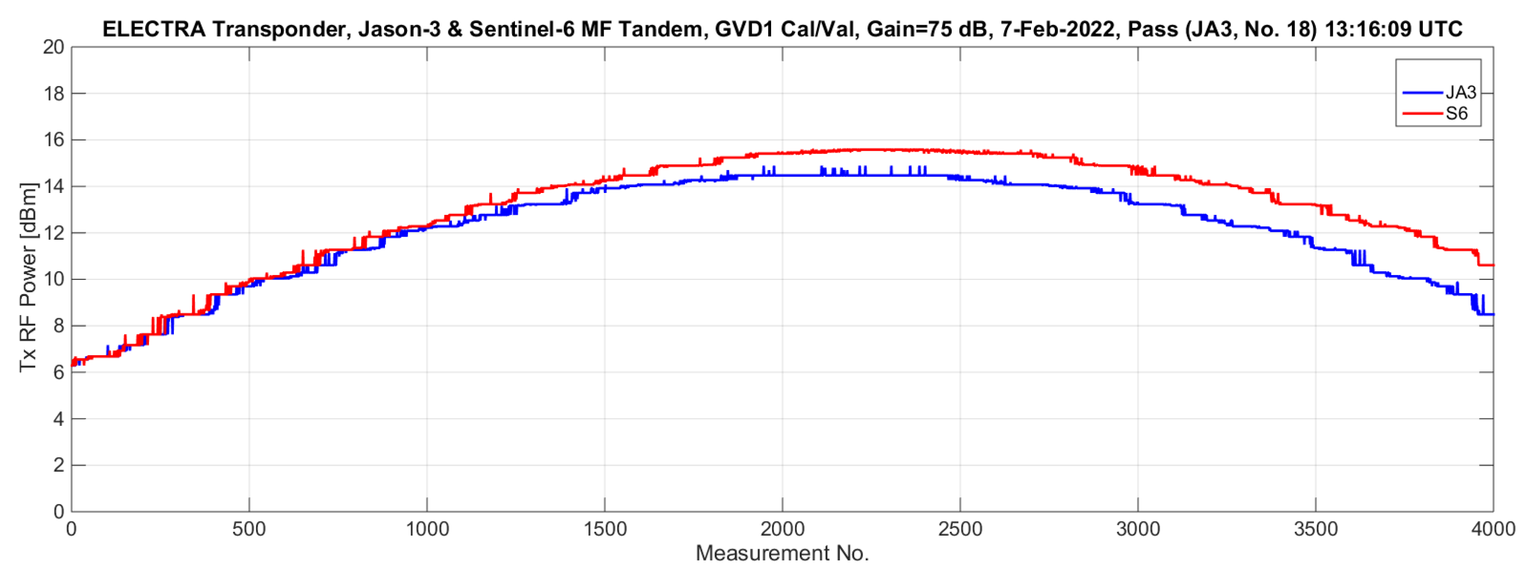
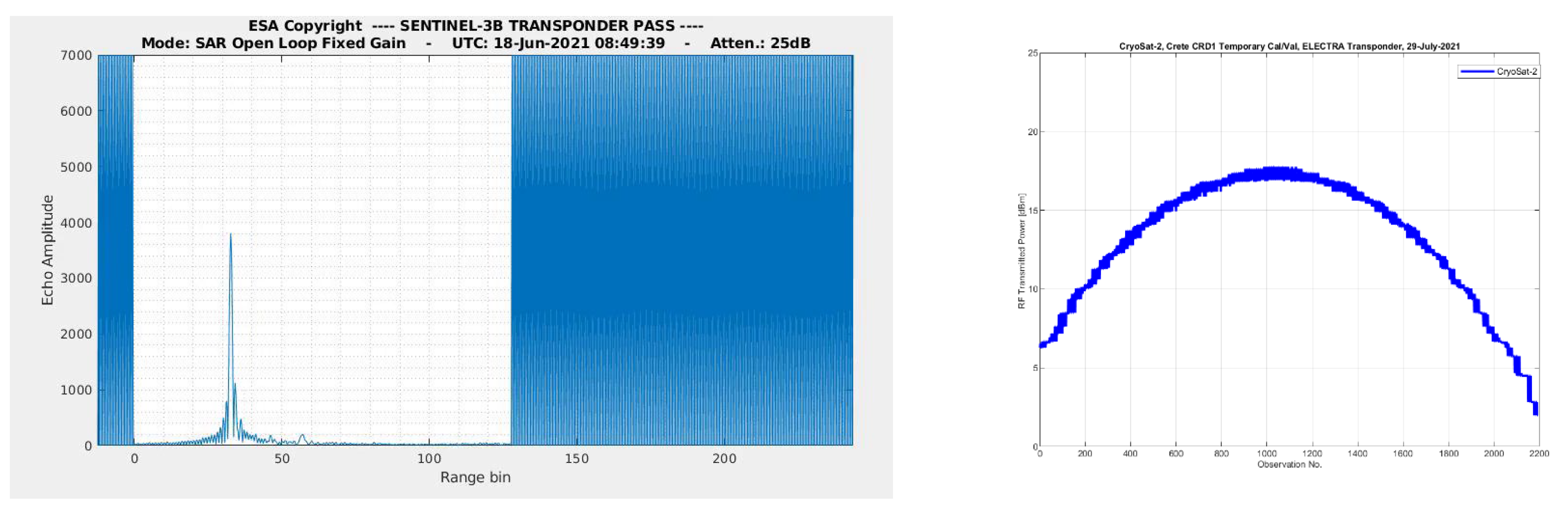
  • Signal recording. The ELECTRA transponder is capable of recording signal power at 1 μs sampling steps at the output of its amplification stage (Figure 6).
The ELECTRA transponder consists of the following components: (1) the electronics, (2) the microwave antennas, and (3) the mechanical support structure to mount the electronics parts and the antennas (Figure 7). All these components are custom-made and tailored to meet strict specifications and requirements prescribed by ESA. Each component was independently manufactured, and all components were assembled before characterizing and testing the integrated transponder unit.
The ELECTRA transponder is a prototype instrument. As such, it had to be calibrated and characterized in different specialized facilities. A series of characterization tests was carried out, such as (Figure 8) the following:
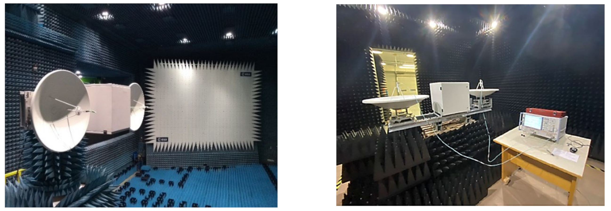
  • Antenna isolation. Isolation measurement of transmit and receive transponder antennas together with their associated Radio Frequency (RF) cables (Figure 8). The isolation achieved was at the level of 110 dB.
  • Antenna alignment. Measurements were performed to align the antennas to the boresight with an accuracy of about ±0.1° and characterize their radiation pattern after proper alignment.
  • Amplifier stability. Two sets of tests for the stability of the integrated transponder with the RF Unit connected to the transmit and receive antennas were carried out. The first set was performed with the transponder at a steady state with the maximum amplifier gain. The second test was the same as the first but at a transient state; sending a pulse with a maximum amplifier gain of 80 dB, we were able to inspect for any signs of amplifier instability in the time domain. The stability of the amplifier chain was measured to ±0.1 dB.
Following laboratory characterization of the ELECTRA transponder, its performance was evaluated, at first, in the field at a temporary location in Crete before its final installation at the permanent GVD1 Cal/Val site on Gavdos Island. The temporary Cal/Val site in Crete, called CRD1, was selected, close to Sentinel 3-B Pass No. 70 and CryoSat-2 ground tracks (Figure 9). Two transponder calibrations were carried out: on 23 July 2021, 19:58 UTC during the Sentinel-3B Pass No. 70 and on 29 July 2021, 15:31 UTC during the CryoSat-2 overpass. Both tests were declared successful (Figure 10). After that field testing, the transponder was ready and moved to its permanent site, GVD1, in Gavdos.

2.1.3. The GVD1 Transponder Cal/Val Site on Gavdos Island

The transponder was finally established at the GVD1 Cal/Val site early in October 2021. The land of the GVD1 Cal/Val site has been the property of the Technical University of Crete since 30 October 2003. A permanent GNSS station (i.e., GVD0) and a meteorological station had been operating at this location continuously since 2003. Also, for a decade (2003–2014), a DORIS (Doppler Orbitography and Radiopositioning Integrated by Satellite) beacon (called GAVB) was operational at this Gavdos location, allowing GNSS-DORIS intercomparisons (site velocities and tropospheric delay estimation) [27]. As a consequence, there is a historic record available for that site in terms of precise positioning along with its tectonic deformation monitoring.
In 2021, amid the Covid-19 pandemic, the GVD1 Cal/Val infrastructure and instrumentation were upgraded with (a) a 50 m2 building to host the transponder and its ancillary equipment and to protect key instrumentation against environmental conditions, (b) a dome to protect the ELECTRA transponder that can open and close when a satellite observation takes place, (c) a second GNSS receiver and meteorological station pair (GVD2) along with a DORIS beacon, (d) mains and a backup power supply system, (e) secure and uninterrupted communication links via dedicated internet links and 4G mobile, (f) lightning protection, etc. (Figure 11).
In 2023, a new DORIS station (named GAVC) equipped with a fourth generation beacon was installed along with a GNSS real-time station (GVDG) that will be part of the IGS network. In addition, on the occasion of this installation, a high-precision local tie survey including high-precision levelling between the transponder Cal/Val site (GVD1) and the sea-surface Cal/Val site (GVD8) was carried out by the IGN surveying team in order to provide high-accuracy height differences between all instrument reference points.
In the context of the described transponder upgrade of the PFAC infrastructure, an additional sea-surface Cal/Val site was also established in the southwest part of Crete to calibrate Sentinel-3A, Sentinel-3B, and Sentinel-6 MF. A description of this site follows.

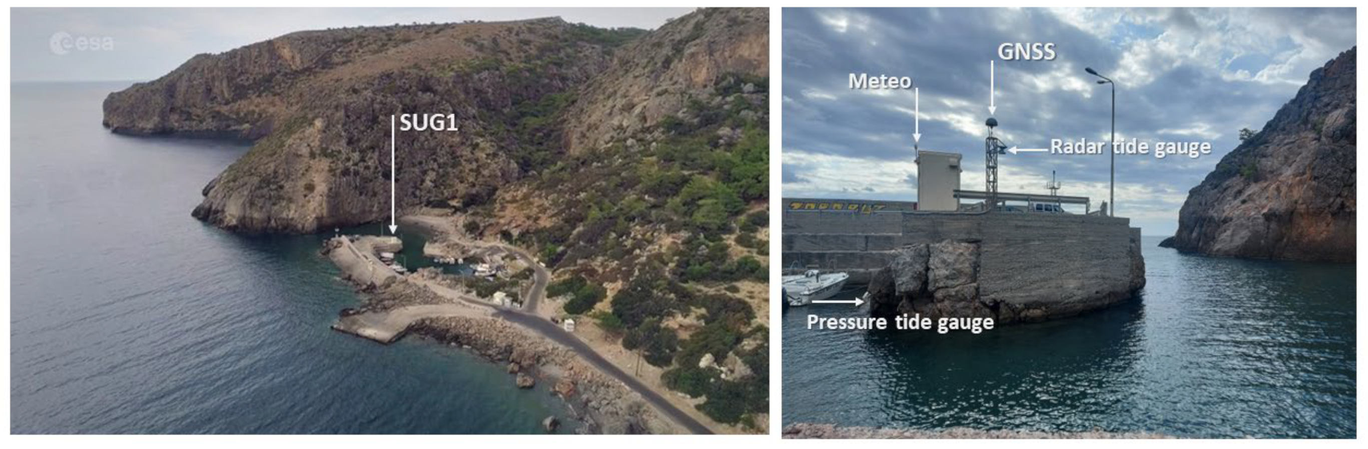
2.2. The SUG1 Sea-Surface Cal/Val Site in Crete

Intercomparisons of the Cal/Val results derived by diverse techniques, instrumentation, locations, and settings comprise the building blocks of the foundation of the FRM strategy. To follow that principle, it was decided to establish a new sea-surface Cal/Val site about 11 km south of the CDN1 transponder Cal/Val (Figure 4 and Figure 5) site, at a small fishing harbor, south of Crete. The new site is called SUG1 and it is such that at least three satellite altimeters could be calibrated with sea-surface techniques only a couple of seconds apart before or after a transponder calibration takes place in the mountains of Crete at the CDN1 Cal/Val site. This SUG1 Cal/Val site serves the Sentinel-3A with its ascending Pass A14, Sentinel-3B with the descending Pass D335, Sentinel-6 MF with its descending Pass D18, as well as the CryoSat-2 (Figure 1 and Figure 4) with several passes.
The SUG1 Cal/Val site is equipped (Figure 12) with one radar and one pressure tide gauge, a GNSS receiver, and a meteorological station. The site has been continuously operational since 5 March 2021.

2.3. The Overall PFAC Ground Reference Instrumentation

Table 1 summarizes the infrastructure and instrumentation of the PFAC utilized for the scientific analyses presented in the following sections. Data from these remote sites are automatically transferred via appropriate communications links (i.e., satellite, dedicated wireless links, 4G) for archiving at the Operations Control Center hosted on the Technical University of Crete premises.
This section has presented recent work made by the PFAC team and ESA to upgrade the ground reference instrumentation in Crete and Gavdos and, thus, to safeguard the Cal/Val services provided by this research infrastructure. In the following section, reference measurements, products, and models applied to carry out satellite altimetry Cal/Val activities are described.

3. Quality Control of Ground Reference Observations and Satellite Products

The bias of satellite altimeters is determined at the PFAC infrastructure, using independent and diverse Cal/Val techniques. Each technique is devoted to calibrating one or more satellite observations and/or products. For example, transponder calibration is applied to determine range bias, and sea-surface calibration is to monitor the quality of the altimetric product of the sea-surface height but also to determine its bias. Still, the existing GNSS network operating in coastal areas is there to validate observations of the onboard radiometer in relation to the satellite’s proximity to land. Finally, crossover analysis directly compares satellite measurements made by different altimeters when satellites overfly at the same location at sea and within a time interval of 1–2 days. This last Cal/Val technique does not require any ground measurements but relies only upon satellite observations.
The way that these Cal/Val techniques are engaged in the PFAC along with a detailed analysis of uncertainty constituents has been described in [15]. Here, we examine the sensitivity and dependence of each Cal/Val technique upon certain unknown factors and parameters of ground reference observations.
For example, the transponder’s internal delay is a parameter whose chosen value along with its uncertainties propagates into the Cal/Val values. The derived signal delays in the ionosphere and troposphere also control the results of the transponder bias. The absolute positioning of the measuring points of reference’s ground instrumentation also regulates the outcome of calibration, be it transponder or sea-surface height. Likewise, in sea-surface calibration, water level observations made by tide gauges, employed reference surfaces (i.e., geoid, mean dynamic topography, mean sea surface) related to transfer heights from the coast to the open ocean, and many more factors carry their uncertainties to the final results for the sea-surface height bias.
To realize and match up to the fiducial reference measurement status, continuous monitoring of ground instrumentation is carried out. In the following sections, evidence of FRM compliance for the PFAC key instrumentation as it takes place on an operational basis is given.

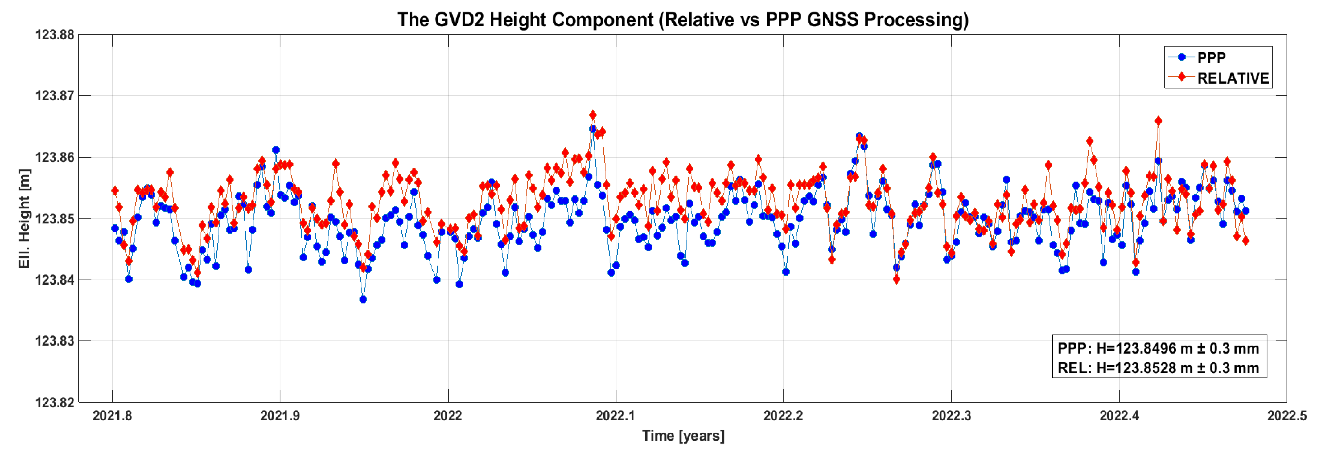
3.1. Absolute Positioning

The two transponders in Crete and Gavdos Island and the other sea-surface Cal/Val sites are supported by the simultaneous operation of two GNSS stations at each individual site (Figure 13). Each GNSS receiver is collocated and connected with a weather station, recording atmospheric temperature and pressure, relative humidity, and wind speed and direction. These meteorological parameters are used for the determination of the wet troposphere delay derived from GNSS observations.
Satellite observations recorded by each GNSS station are processed using diverse techniques (i.e., relative positioning [28], precise point positioning with ambiguity resolution (PPP-AR) [29], etc.). But what final values for the transponder location are fed into the calibration process? First, a spirit levelling survey is periodically (i.e., semi-annually) carried out to determine height differences between each GNSS antenna reference point and that of the transponder. Thus, the collocated GNSS stations are tied with the reference plane of each transponder. For example, at the CDN1 Cal/Val site, four independent solutions for transponder coordinates are produced: coordinates with relative and precise point positioning for the CDN0 and CDN2 GNSS stations.
The ellipsoidal height in ITRF2020, h T R P , R , of the reference point of the CDN1 transponder is derived as a weighted average between the two determined GNSS heights, per processing, applied as
h T R P , R = w 0 , R · h 0 , R + w 2 , R ·   h 2 , R ,
where h T R P , R is the determined ellipsoid height of the transponder point, using relative positioning, and based on heights coming from the GNSS stations of CDN0 (i.e., h 0 , R ) and CDN2 (i.e., h 2 , R ) and after their transfer through precise levelling from each station to the transponder reference point. The coefficients w 0 and w 2 are weights applied to the respective heights of the CDN0 and CDN2 stations. Weights are expressed as the reciprocal of the squared dispersion of the relative GNSS processing, in this case for each specific GNSS station. The same procedure is applied for the determination of the height of the transponder reference point for other GNSS processing, such as precise point positioning (PPP), in the form of
h T R P , P P P = w 0 , P P P · h 0 , P P P + w 2 , P P P ·   h 2 , P P P ,
So, after this procedure, two heights for the transponder reference point and two uncertainties arise. The final transponder height and its combined uncertainty (at 68% confidence) is an integration of both procedures. In this case, the uncertainty for the transponder ellipsoidal height amounts to u 1 = ± 2   mm . An example of the positioning results, in the reference frame of ITRF 2014, along with their deformation velocities, for the GVD2 permanent station in Gavdos’ transponder are given in Table 2. Figure 14 shows the time variations for the height coordinates of the same GVD2 station in Gavdos.

3.2. Transponder Internal Delay

An active transponder receives, amplifies, and transmits back to the satellite the radar signal originally transmitted by the satellite altimeter. In this process (receive–amplify–transmit) there is a group delay of the satellite signal introduced by the transponder’s electronics, its cables, and the transmit/receive antennas. Both the CDN1 transponder in Crete and the GVD1 transponder in Gavdos have been fully characterized not only at the Compact Payload Test Range facilities in the European Space Agency, the Netherlands, but also in specialized facilities in Athens, Greece (Figure 8). The uncertainty in the determination of this internal delay of the RF transponder is estimated to be within u 2 = ± 10 30   ps [7]. In the field, transponder electronics may vary this estimated internal delay depending on the operating conditions (i.e., temperature, humidity) [30].

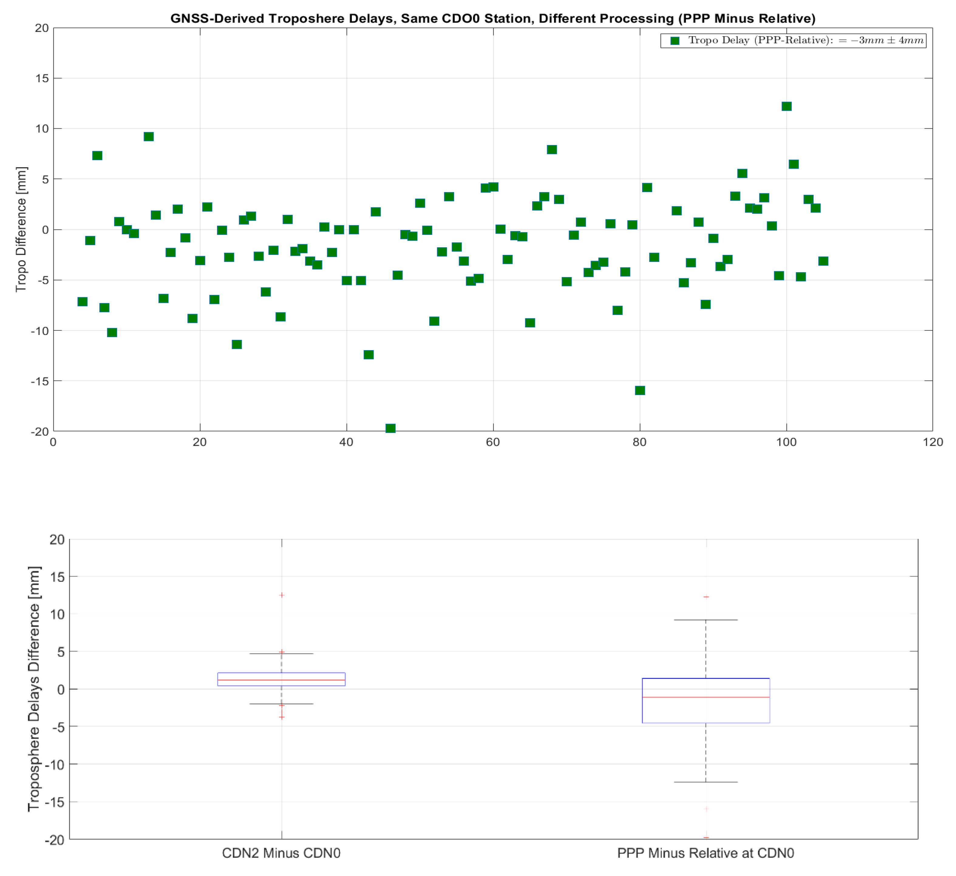
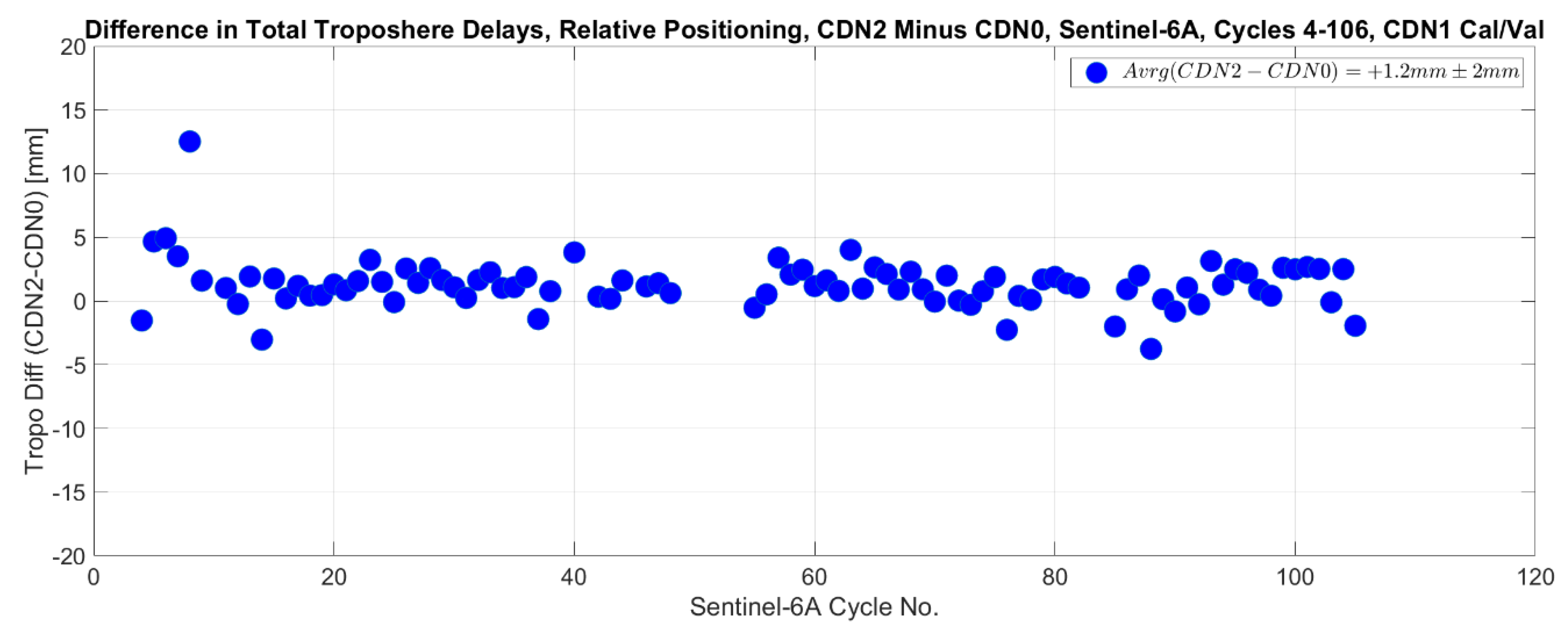
3.3. Atmospheric Delays of Satellite Signals

The atmosphere causes a bending of the path of satellite signals and changes their propagation velocity. This leads to atmospheric path delays that need to be accurately estimated as they influence both absolute positioning and the measurement of altimeter ranges. Signal delays of the dry troposphere are of the largest magnitude but can be accurately modeled. In contrast, the wet troposphere delay varies abruptly, and its estimation becomes a challenging task.
In satellite altimetry calibration, it is the total troposphere delay of altimeter signals that is of particular concern. Its magnitude corresponds to the delay that altimeter signals experience passing through the troposphere.
Let us examine the values of troposphere delays as determined by two nearby GNSS stations, about 7 m apart, at the transponder Cal/Val site in Crete. For each Sentinel-6 MF overpass, the total tropospheric delay has been derived through GNSS observations made at these two stations, CDN0 and CDN2. Each station operates different receivers, antennas, and cables. The differences in tropospheric delay between those coming from the CDN0 and CDN2 stations (CDN2 minus CDN0), using the same GNSS processing technique (e.g., relative positioning), are within ±5 mm (except Cycle 8, classified as outlier) and have an average value of +1.2 mm.
As seen from Figure 15, there are no values for Cycles 49–54 (March–April 2022). This is because of a malfunction in the antenna cable of the CDN2 station that led to no recording of the GNSS observations during this period. However, as can be seen later in the Results Section, this instrument failure had no impact on transponder Cal/Val services, as the other GNSS station (CDN0) worked normally.
By the same token, let us evaluate variations in troposphere delays derived at the same GNSS station but implementing different GNSS processing. The differences in the total tropospheric delays as determined for the CDN0 GNSS station using relative and precise point positioning are illustrated in Figure 16. These differences are within ±10 mm, with an average of −3 mm. The value at Cycle 46 is classified as an outlier.
All previous analysis demonstrates the need for having redundant operating instruments to appraise all uncertainties involved in altimeter calibration.

3.4. Asymmetry of the Transponder-Satellite Waveform

Two typical waveforms are shown in Figure 17. They were created from the altimeter signals arising from the satellite in combination with the ELECTRA transponder system on the ground at the GVD1 Cal/Val site on Gavdos Island. One corresponds to the descending orbit D18 (about 2500 m away from the transponder) and the other to the ascending orbit A109 (500 m from the transponder). It appears that the descending orbit D18 of Sentinel-6 MF shows an asymmetry around the mainlobe. This asymmetry may affect the location of the peak of the mainlobe, which certainly by default defines altimeter ranging. The units of power in both waveform diagrams are in dB and each bin in the horizontal axis corresponds to 0.7 mm in distance steps.
From the two waveform shapes of Figure 17, the following can be observed:
  • The waveform along the ascending orbit A109, with its two sidelobes, appears symmetric around the mainlobe. The difference in power between the left and the right sidelobes is of the order of 0.01 dB. Certainly, there are cases wherein this power difference in sidelobes, laid astride the mainlobe, is more than 0.01 dB in some cycles, but as a general rule, no major shift for the location of the mainlobe is anticipated along this ascending orbit A109.
  • On the other hand, the waveform along the descending orbit D18 appears asymmetric with a difference in power between left and right sidelobes of the order of 3.77 dB, on average. This creates an asymmetry of the mainlobe shape and requires correction, as there is a shift in the origin of range measurement. The mainlobe asymmetry originates from interference generated because of the transponder antenna array with respect to the satellite pass and it happens when the transponder antenna array is almost parallel to the descending orbit. No such case occurs for the ascending orbit A109, where it creates an angle of about 60 degrees with the transponder antenna array.
This signal interference of the transponder has been analyzed, and the generated waveform was simulated in such a way that the location shift of the mainlobe was determined in relation to a symmetric and ideal waveform location. Note that everything below 20 dB in the waveform is neglected as such a power level is infinitesimal and does not cause any distortion. Such a simulated waveform is shown in the lower diagram of Figure 17d. That example creates a sidelobe difference of 3.66 dB followed by a waveform shift from its ideal location and, subsequently, a change in range of 22 mm. The same procedure has been applied to all altimetric ranges produced by the transponder to make up for the waveform distortion.

3.5. Sea-Surface Height at the Tide Gauge Location

At each sea-surface Cal/Val site, water-level observations are generated by a series of tide gauges to determine the absolute height of the site above the ellipsoid. For example, at the Gavdos sea-surface Cal/Val site, four tide gauges of different technology and makes have been operating continuously to produce, as a rule, four different observations (Figure 18). But one value must be delivered out of these four observations. Next, these measurements are connected to the absolute heights of certain benchmarks in the surroundings, whose heights were determined by GNSS positioning and precise levelling. Yet, to arrive at a single, reliable, and objective value for the sea level at the Cal/Val site at the time of a satellite pass, not only must the quality of water level observations be continuously monitored, but also the different tide gauge observations have to be properly integrated. A single value for the sea-surface height at the Cal/Val site and at the time of a satellite overpass is, thus, produced and subsequently fed into the processing for sea-surface calibration. In this process, several uncertainty constituents are involved. Let us examine the most significant ones.

3.5.1. Determination of the Zero-Point of a Tide Gauge with Camera Monitoring

Irrespective of the measuring technique employed (i.e., radar, acoustic, pressure, etc.), each tide gauge determines the vertical distance between a reference point on its sensor and the water level. This reference point on the tide gauge is of utmost importance as at times its location does not coincide with the origin of observations, or it may change over time, especially in radar measurements. To transform tide gauge observations to sea-surface heights, this zero-point on the sensor must be tied to the coordinates of collocated GNSS reference stations. Tying is accomplished by spirit levelling that accurately (±0.5 mm) establishes the height difference of the zero-point on the sensor with respect to the GNSS antenna reference point. It is, thus, of importance to accurately define this tide gauge reference point and its uncertainty.
A technique for the field characterization and determination of the zero-point of a tide gauge has been devised. In this technique, a tide pole is installed next to the operating tide gauge and its readings with respect to the sea water are monitored by a camera. A digital camera is placed in front of the tide pole to capture high-quality images of water levels and the pole readings every 1 min, for example (Figure 18), depending on tidal variations. Camera images are then processed in relation to the captured readings of the tide pole. Considering that the tide pole is tied to the benchmarks in the vicinity of the Cal/Val site and the GNSS reference station, the “true” sea-surface height is, thus, determined and compared instantaneously with the observations made by the tide gauge.
Tide pole observations acquired by the camera result in accurately (±1 mm) measuring the instantaneous sea-surface height on-site and constitute a realization of the produced tide gauge observations [31].
Figure 19 presents the differences in hourly water level measurements as determined by the Gavdos tide gauges and the tide pole readings during an experiment carried out in June 2021. It seems that for this specific period and under the same weather and sea state conditions, the KVR3, KVR6, and KVR7 tide gauges have an average offset at the mm level (+1 mm, −6 mm, and +4 mm, respectively), whereas the KVR4 sensor shows an average offset of −13 mm. This offset is then adjusted in the water level records to produce zero-leveled results for each tide gauge.

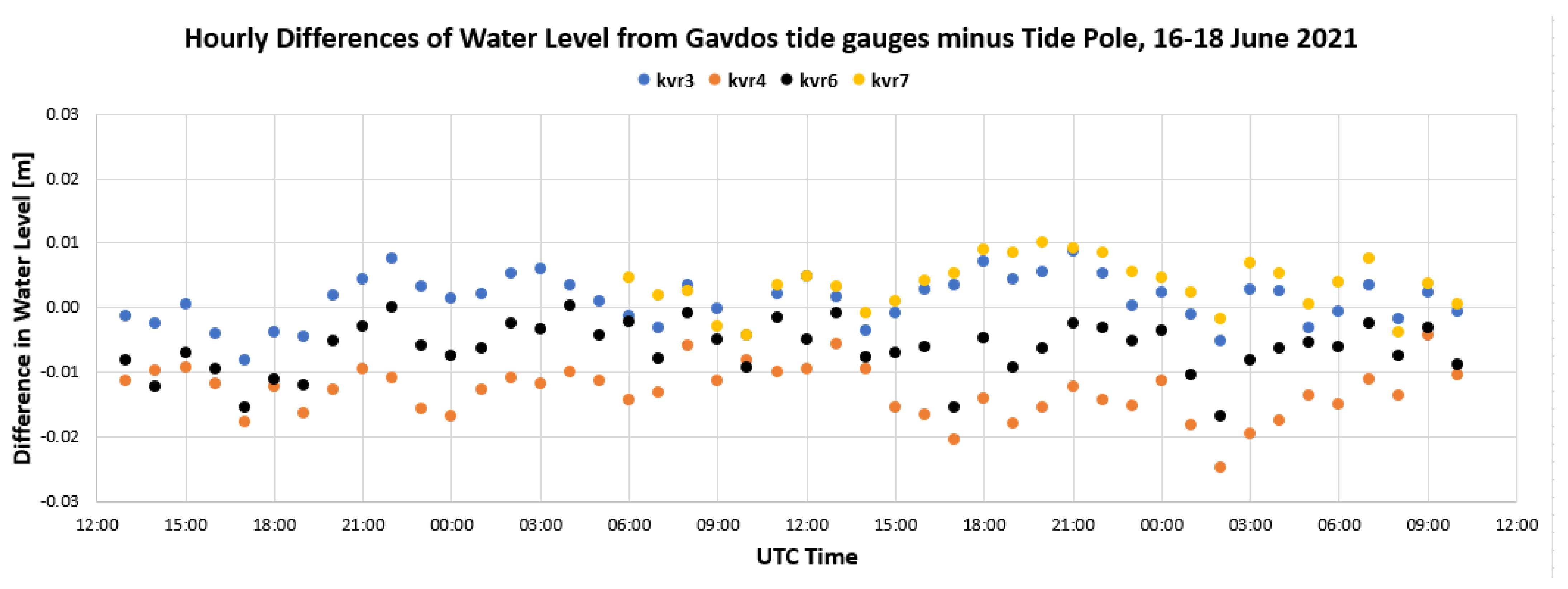
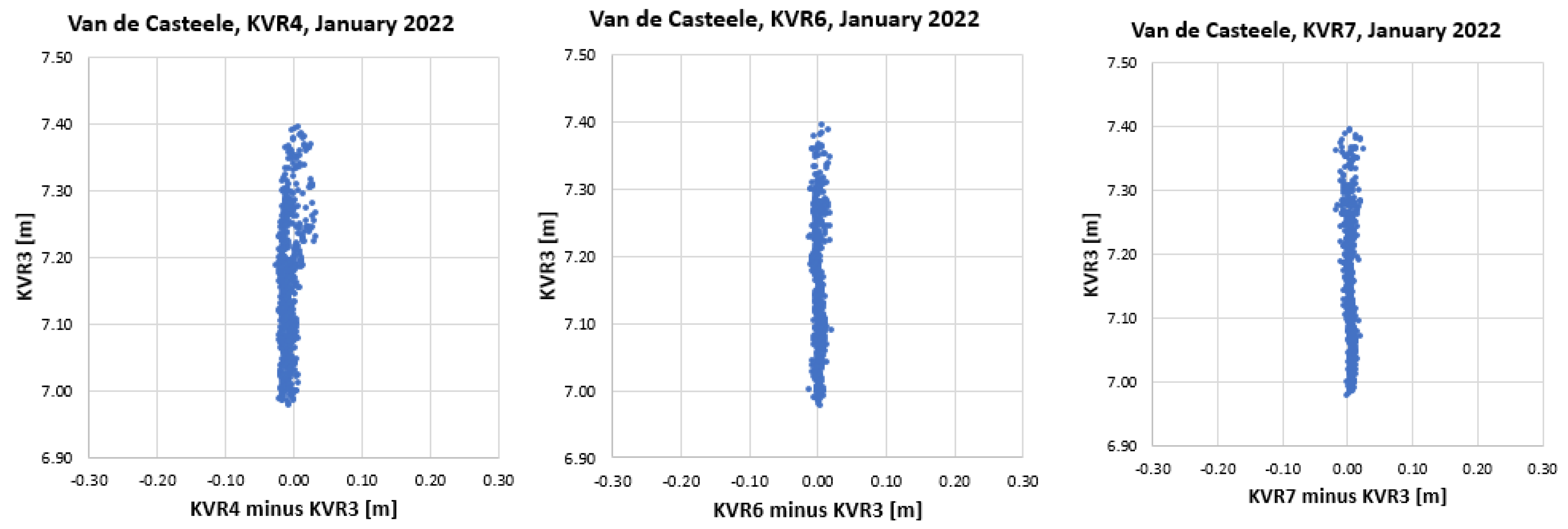
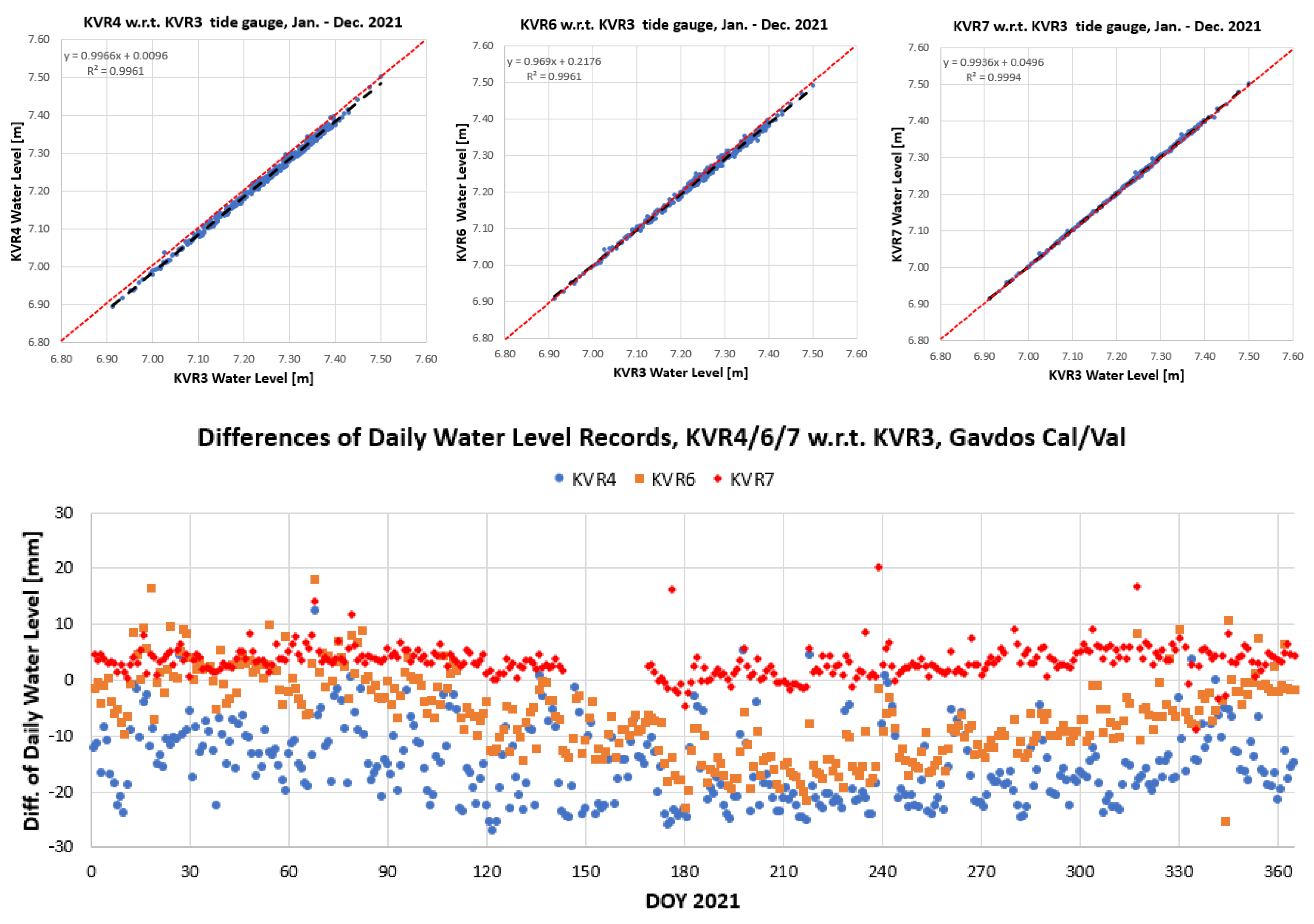
3.5.2. Validation with a Reference Sensor

One of the methods routinely used to monitor the tide gauge time series is to examine them with respect to a standard reference instrument [32]. In the PFAC, the performance of the collocated tide gauges is evaluated using a Van de Casteele diagram [33]. This diagram represents the difference in sea level between an instrument under evaluation and that of a reference instrument. The most appealing aspect of this diagram is its ability to offer a visual inspection for direct identification of a potential bias/problem in just one tidal cycle. In the PFAC, this analysis is carried out monthly. Figure 20 shows these Van de Casteele diagrams produced for January 2022 in Gavdos with respect to the reference tide gauge, that of KVR3.
Figure 21 presents the scatterplots of the daily water level records of each tide gauge (KVR4, KVR6, KVR7) with respect to the reference KVR3 sensor for a period of one year. It can be seen from Figure 21 that the performance of all tide gauges is within specifications (±1–2 cm).

3.5.3. Final Sea-Surface Height

The acquisition of sea level measurements from several sensors enables their comparative assessment and the identification of any instrument offsets, drifts, or periodic variations. It also ensures the reliability of the estimation of sea-surface heights at the Cal/Val site during the time t k for a satellite calibration. The estimation of the sea-surface height, h 0 ( t k ) , from several tide gauges is performed as follows.
At first, a sample of 24 h duration (one day) is extracted from the original time series of tide gauge observations, and this sample is centered at the time of the satellite pass, t k . This time t k corresponds to the time of the closest approach of the satellite overpass over the specific Cal/Val site. For each truncated sample, coming from a certain tide gauge, j , the sea-surface height, h 0 , j t k , is determined by the following:
h 0 , j t k = Δ h j t k + l j t k + d l D A C , j t k + d l T I D E , j t k ,     j = 1 , 2 , 3 , 4 .
where Δ h j t k is the height above the ellipsoid of the reference point of the j t h tide gauge at time t , l j ( t k ) is the tide gauge observation, which is the vertical distance (height difference) from its reference point to the instantaneous sea surface, d l D A C , j ( t k ) is the dynamic atmospheric correction (DAC), and d l T I D E , j ( t k ) is a tidal model correction to compensate for any high-frequency noise.
The time series h 0 , j t k for the j -th tide gauge sensor, is fitted by a four-degree Fourier series, denoted by h ^ 0 , j . Figure 22 shows such a fitted model for the four tide gauges in Gavdos Cal/Val site, along with the original measurements, the fitted model, and its residuals. This fitted model for the 24 h time series mitigates any high-frequency noise and results in a smoother time series for h 0 , j t k . The final ellipsoidal height of water surface h 0 t k at time t k is derived using a weighted average of h ^ 0 , j ( t k ) , as:
h 0 t k = w 1   h ^ 0,1 t k + w 2   h ^ 0,2 t k + w 3   h ^ 0,3 t k + w 4   h ^ 0,4 t k [ w 1 + w 2 + w 3 + w 4   ]
The weight w j in Equation (2) represents, in this case, the inverse of the root mean squared error of the fitted Fourier series model on the original observations, i.e.,
w j = 1 / { Ε h ^ 0 , j h 0 , j 2 , }
where Ε · denotes expectation. Nonetheless, several other ways to represent weights and individual contributions of each sensor could be chosen by selecting various scale estimates for the tide gauge observations [16,34]. This previous development of how to handle four tide gauges with different uncertainties demonstrates the need for redundant sensors and observations in support of the FRM strategy requirements.

3.6. Reference Surfaces for Sea-Surface Calibration

Another major source of uncertainty in the estimation of the sea-surface height (SSH) bias is the selected reference surface to transfer the water level at the Cal/Val site to the open ocean where satellite measurements are made. Global and/or regional models for the geoid and the mean dynamic topography may be selected as reference surfaces for this connection. Regardless of the reference surface implemented, it is the sea-surface height difference, along with its associated uncertainty, between the location of the Cal/Val site and the open sea that is of utmost importance for calibration.
To appreciate the amount of confidence to be placed in the selected reference surface, we have chosen a few geoid models, as examples, to demonstrate the uncertainties involved in this height transfer and connection. Figure 23 presents the determined bias in sea-surface height for Sentinel-6 MF along its descending Pass D18 from south Gavdos to Crete (only latitude variations are shown in Figure 23), using Cycle 13 with different geoid models. The global gravity geoid models of XGM2019 [35], EGM2008, EIGEN-6C4 [36], and GECO [37] have been chosen for comparison, in this example.
At certain calibrating regions, the determined bias of Sentinel-6 MF can differ by up to 8 cm between various geoid models, for this cycle. Similar results are obtained for other cycles and altimetry missions. Conclusions about satellite bias may, thus, change considerably. No meaningful comparisons could be drawn among these models within a set of calibration requirements. Results are highly dependent upon the chosen geoid model, the specific location where calibration takes place, and certainly upon the distance from the Cal/Val reference site (here, Gavdos). Such bias profiles clearly manifest imperfections of the chosen global gravity geoid models to reliably transfer heights from the Cal/Val site to the open ocean and the unsuitability of these global models to clearly provide an articulated ground truth for calibration.
The previous analysis presents the crucial need for an accurate geoid model (and certainly the mean dynamic topography) to be operationally meaningful for sea-surface calibration, and justifies the large uncertainties presented for the regional geoid model in the FRM uncertainty estimation (Table 3).

3.7. Processing Baseline of Satellite Products

Satellite products are commonly provided at different times, depending on the processing stage implemented. For example, products of Sentinel-6 MF have been released at various time periods, commonly identified as the “baseline collection field”, designated as F01, F02, F03, etc. Such product releases (the latest report is F08 and can be found in https://eumetsatspace.atlassian.net/wiki/spaces/PQ/pages/1773928450/Sentinel-6+reports (accessed on 2 January 2024)) have been regularly updated whenever changes are made to the entire Sentinel-6 MF satellite and/or ground segments that significantly impact data quality and performance.
To assess the different releases of processing versions for Sentinel-6 MF, sea-surface heights of Sentinel-6 MF were compared against Jason-3, using low-resolution (LR) and high-resolution (HR) products. Jason-3 is used here as baseline reference. Figure 24 illustrates the difference in sea-surface heights between Sentinel-6 MF and Jason-3 when both satellites flew in tandem. The assessment took place over an uncontaminated ocean region of about 15 km, south of Gavdos and extending over an ocean length of about 8 km. Different releases of satellite products are noted on both diagrams with respect to Jason-3 cycle numbers. Comparison is made over Jason-3 Cycles 179 (18 December 2020) up to 223 (27 February 2022) and along the descending Pass D18 and the ascending Pass A109, all referenced to the Gavdos Cal/Val site.
Each point in Figure 24 represents an average value in the determined differences in sea-surface heights ( N 17 20   points) based on a different processing version for Sentinel-6 MF, with Level-2 data. Jason-3 products refer to GDR-F data products.
It can be seen from Figure 24 that each processing version of Sentinel-6 MF seems to produce systematic differences with respect to Jason-3. It is, thus, vital for each Cal/Val site to report the specific release of the satellite product (e.g., GDR-F for Jason-3, Level-1/2 for Sentinel-3 and Sentinel-6 MF, etc.) used for their analyses, as any change in the orbital, geophysical, and atmospheric models and procedures may impact the final Cal/Val results [38]. Thus, the specific processing release of Sentinel-6 MF may influence the final Cal/Val results.

3.8. Fiducial Reference Measurement Uncertainty

The previous analysis provided evidence for how the uncertainty is determined for the most influential constituents and how it is evidently propagated to the final transponder and sea-surface calibration. A more complete analysis of this uncertainty estimation has been presented in [13].
For a given group of Cal/Val sites (i.e., sea-surface, transponder) and setting, the FRM uncertainty of each Cal/Val site is expected to be practically the same. This is because the principal uncertainties, such as the transponder’s internal delay or the reference surfaces, dominate the overall FRM uncertainty [15,39]. In this respect and following the previous development in [15,40], the FRM uncertainty for sea-surface Cal/Val is reported to be ±45–50 mm, whereas the FRM uncertainty for transponder calibration is ±30–35 mm.
Table 3 shows how the uncertainty budget is calculated based on the individual uncertainty for each constituent that contributes to the final transponder or sea-surface calibration results (Table 3). This table reports standard uncertainty at the 68% confidence level.

4. Results

This section presents the results of transponder and sea-surface calibrations for the radar altimeters onboard the Sentinel-6 MF and Sentinel-3A/B satellites. It also reports the CryoSat-2 results with sea-surface Cal/Val and on the performance of Jason-3 throughout its operational and tandem phase (17 January 2016 till 7 April 2022), that is, from its launch up to the point before entering its geodetic orbit [41]. Altimeter biases have been determined using the PFAC ground infrastructure in Crete and Gavdos Island.

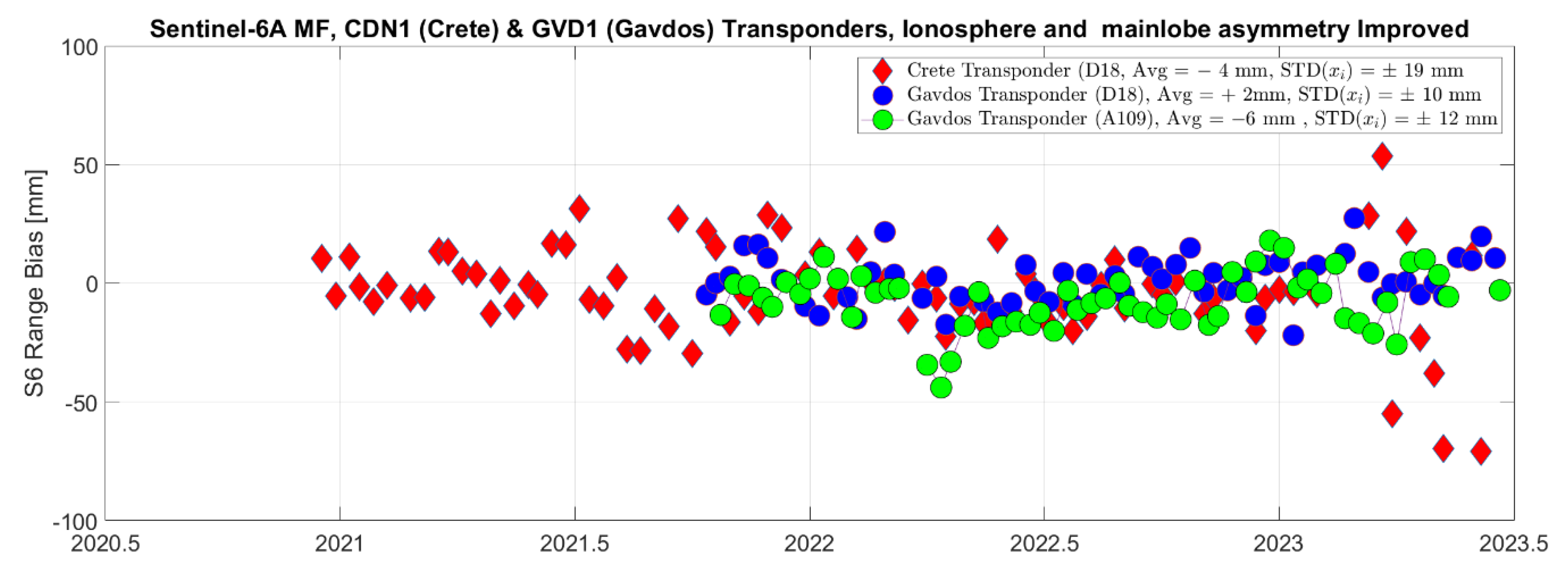
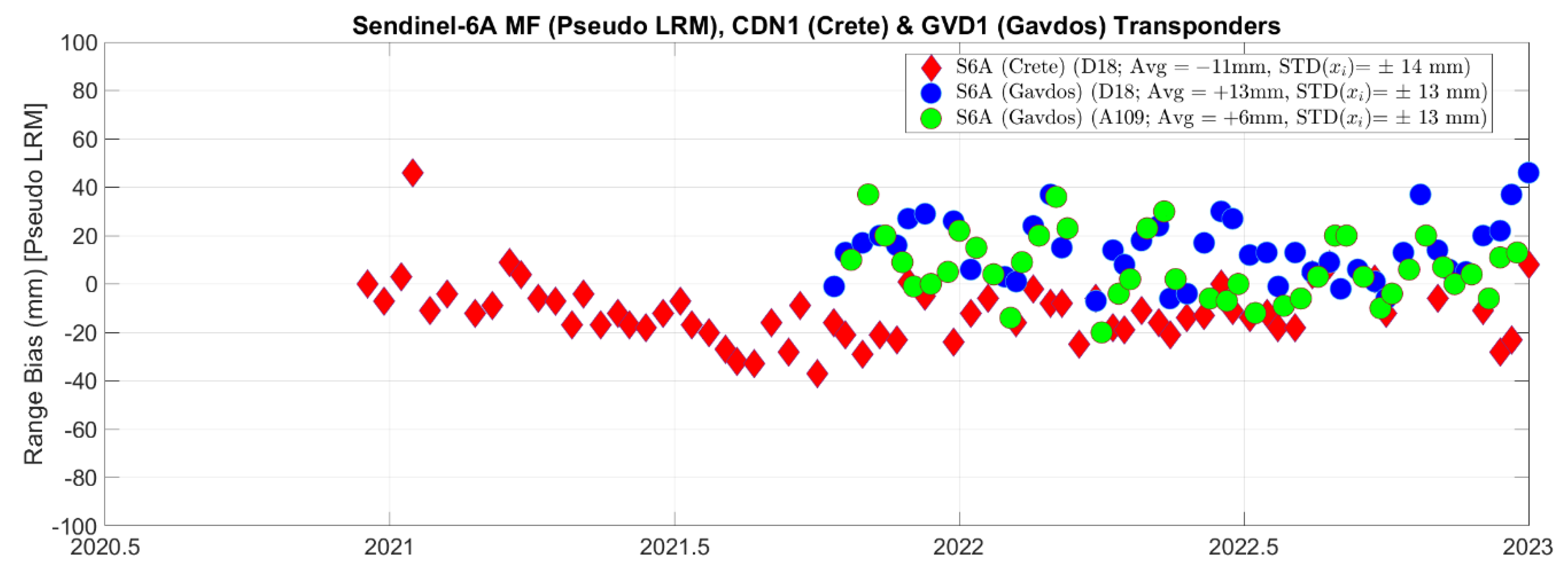
4.1. Sentinel-6 MF Transponder Cal/Val Results

Figure 25 presents the Sentinel-6 MF range bias, as determined using the two transponders (CDN1 in Crete and GVD1 in Gavdos), with its ascending pass A109 and descending Pass D18. The results shown incorporate an improved ionosphere delay, derived out of the GNSS network operating next to the transponders, and include reductions for the asymmetry of the waveform mainlobe, particularly for the descending pass D18.
Range biases of Sentinel-6 MF for SAR observations present an average value of B C D N 1 ; D 18 , S A R = 4   mm   ±   2   mm   ( N = 91 ) with the Crete transponder from 18 December 2020 to 18 June 2023; and a range bias of B G V D 1 ; D 18 , S A R = + 2   mm   ±   1   mm   ( N = 62 )   with the Gavdos transponder from 11 October 2021 till 28 June 2023. Both results were determined almost simultaneously and within 9 s, with different ground instrumentation and settings, as the satellite flew along its descending Pass D18 from the north in Crete and towards Gavdos in the south. Additionally, the ascending Pass A109 produced a range bias of B G V D 1 ; A 109 , S A R = 6   mm   ±   1.5   mm   ( N = 62 )   with the Gavdos transponder during the period of 15 October 2021 to 21 June 2023. Diagrams of the time series of range biases for SAR observations of Sentinel-6 MF are shown in Figure 25. The difference in range biases along ascending and descending orbits is 8 mm, as monitored by the GVD1 transponder.
In the same manner, range biases were also determined using the pseudo-low-resolution mode (Pseudo-LRM) of Sentinel-6 MF. Results are shown in Figure 26. Here, range biases have been determined as B C D N 1 ; D 18 , P L R M = 11   mm   ±   2   mm   ( N = 76 ) in Crete, and B G V D 1 ; D 18 , P L R M = + 13   mm   ±   1   mm   ( N = 42 ) for the descending pass and B G V D 1 ; A 109 , P L R M = + 6   mm   ±   2   mm   ( N = 42 ) for the ascending Pass A109 with the Gavdos transponder. No asymmetrical correction has been applied in these Pseudo-LRM mainlobes of Sentinel-6 MF and not all observations have been processed as Pseudo-LRM observations were not available at the time of processing.

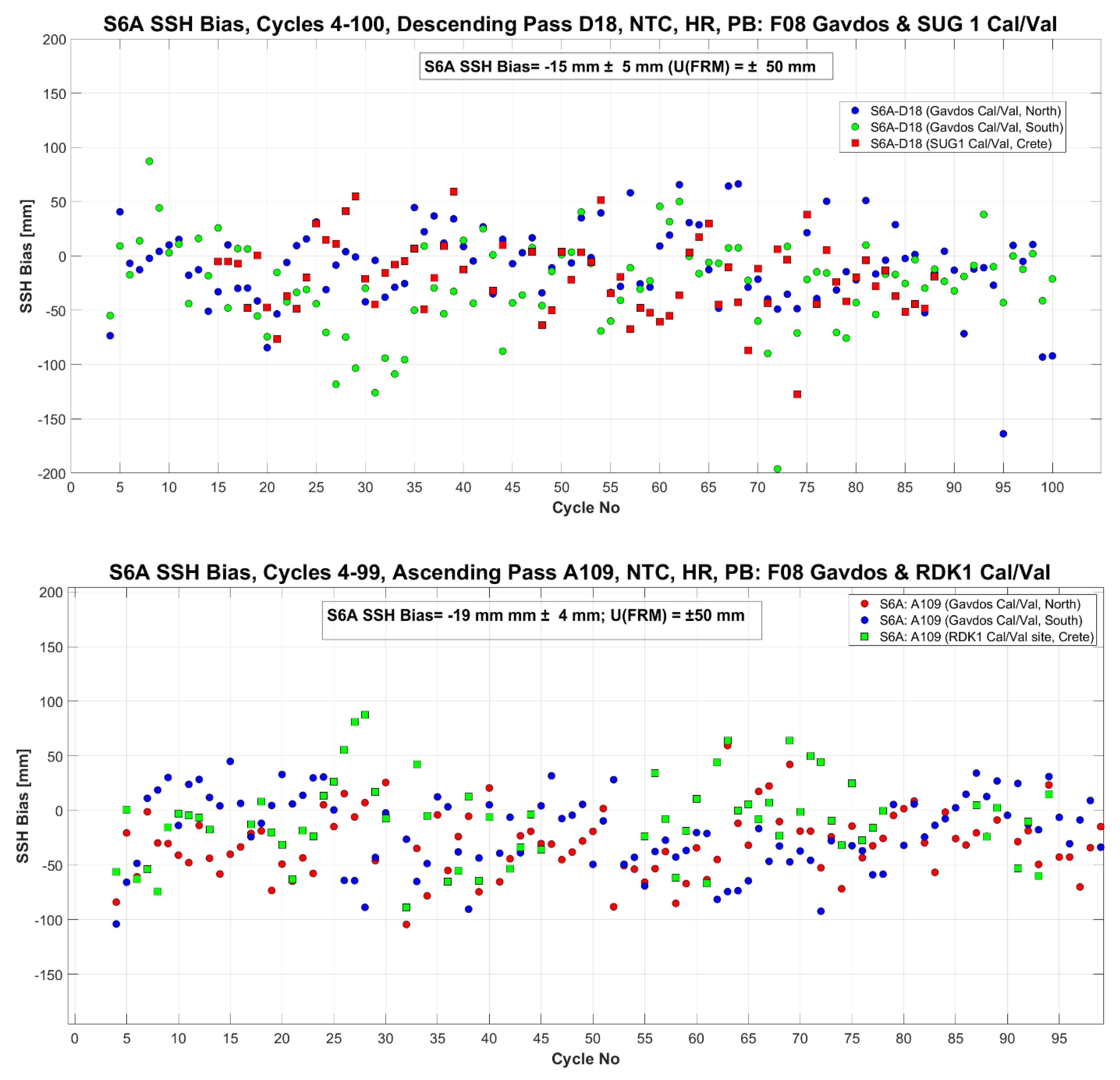
4.2. Sentinel-6 MF Sea-Surface Cal/Val Results

Biases in the sea-surface height were also derived using the satellite products provided by EUMETSAT. To determine bias for the sea-surface height, reprocessed data with processing baseline F08 for Non-Time-Critical (NTC) timeliness for high-resolution (HR) data were used. Three Cal/Val sites, Gavdos (GVD8), RDK1(Crete), and SUG1 (Crete) were used as reference ground sites, and both ascending and descending passes of Sentinel-6 MF, covering cycles 4–99. The results are shown in Figure 27.
With the reference Cal/Val sites of GVD8 in Gavdos and SUG1 and RDK1 in Crete, sea-surface height calibrations were carried out along the descending and ascending orbits of Sentinel-6 MF. The following values have been determined: B G V D 8 , S U G 1 ; D 18 = 15   mm   ±   5   mm   ( N = 96 ) , along the descending Pass D18 and with sites GVD8 and SUG1, and B G V D 8 , R D K 1 ; A 109 = 19   mm   ±   5   mm   ( N = 95 ) along the other ascending pass A109 and the reference sites of GVD8 in Gavdos and RDK1 in Crete. Thus, an average value of B S S H = 17   mm is determined for the Sentinel-6 MF.
Table 4 summarizes all calibration results for Sentinel-6 MF with the transponder and the sea-surface Cal/Val infrastructure. Based on these Cal/Val results, the following points can be given as a summary for the Sentinel-6 MF performance: (1) the Poseidon-4 radar altimeter operations and associated products (i.e., range, sea-surface height) are within mission specifications [42]; (2) both transponders, in Crete (CDN1) and Gavdos (GVD1), deliver similar results with an FRM uncertainty of u(FRM; TRP) = ±30 mm; (3) sea-surface calibrations produce bias results within specifications along with a large FRM uncertainty of u ( F R M ; S S H ) = ± 50   m m . The major contribution of this large uncertainty in the sea-surface height Cal/Val results originates from uncertainties in the local geoid, the mean dynamic topography, and the rapidly changing bathymetry in the region [43]; (4) differences of a few mm between ascending and descending passes, primarily in the transponder calibrations, reflect possible uncertainties in the satellite orbit.

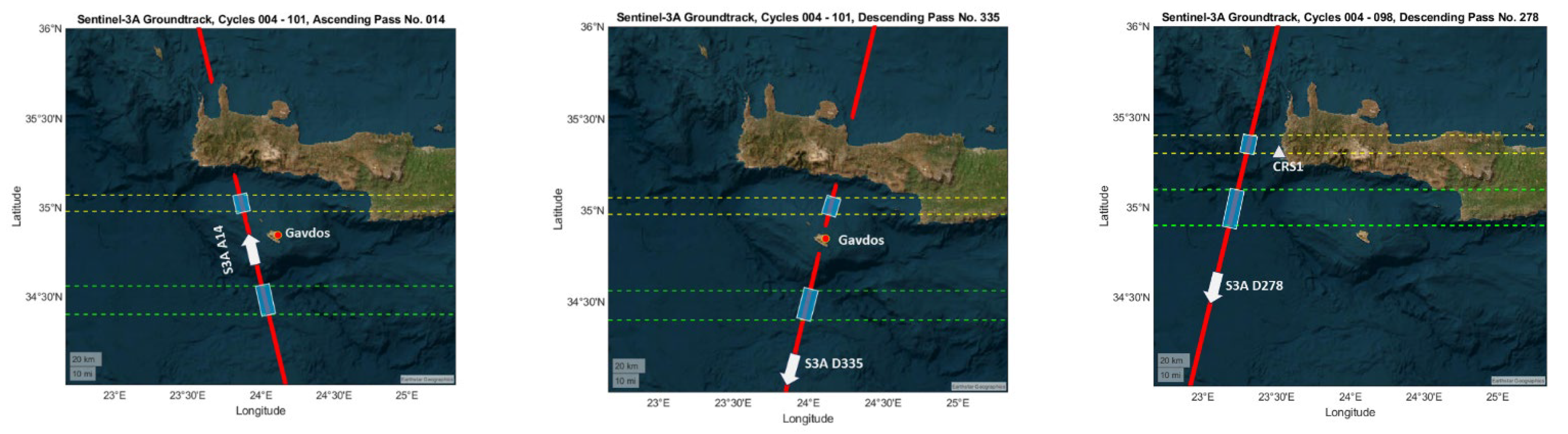
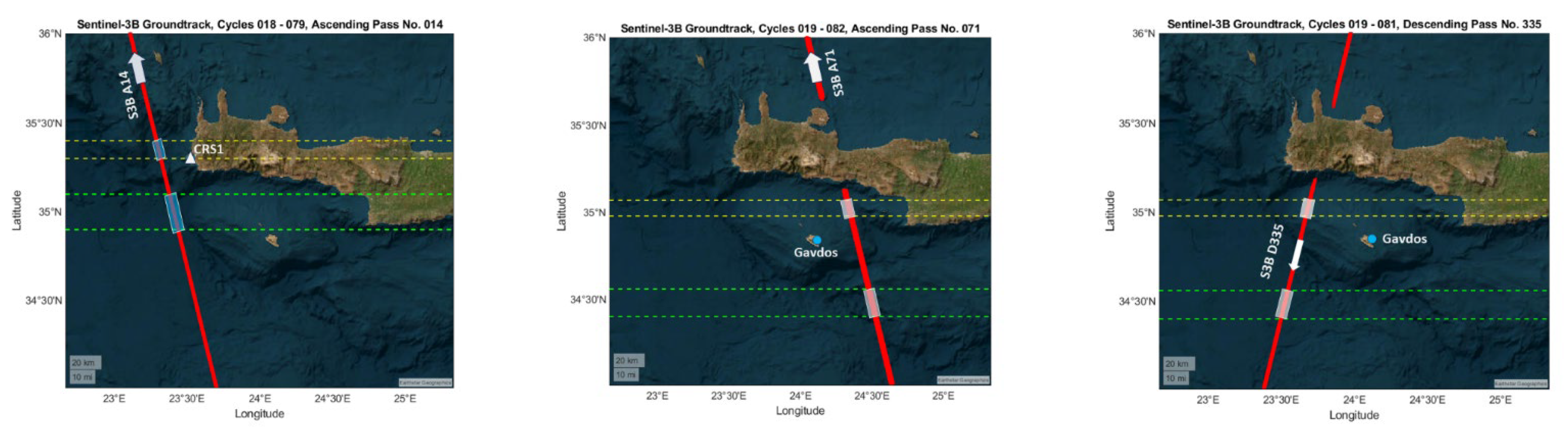
4.3. Sentinel-3 Transponder Cal/Val Results

A unique characteristic of this PFAC ground research infrastructure is that it supports calibration of six (6) Sentinel-3A and Sentinel-3B passes in ascending and descending orbits (Figure 28, upper left image). Redundant Cal/Val sites under Sentinel-3A/B ground tracks offer the advantage of frequent calibration of Sentinel-3A/B and compensate for their relatively long repeat cycle (i.e., 27 days). This setting increases the number of available calibrations and subsequently strengthens the reliability of the delivered Cal/Val results.
Figure 28 presents the absolute range bias results for Sentinel-3A and Sentinel-3B using the CDN1 and GDV1 transponders. Sentinel-3A exhibits an average value for the range bias of B C D N 1 ; A 13 / 14 , S A R = + 1   mm   ±   1   mm   ( N = 78 ) along its ascending pass with the CDN1 transponder in Crete, and a range bias of B G V D 1 ; D 335 , S A R = + 10   mm   ±   1   mm   ( N = 18 ) with the GVD1 transponder in Gavdos.
The Sentinel-3B descending Pass D335 presents a range bias of B C D N 1 ; D 335 , S A R = + 10   mm   ±   1   mm   ( N = 55 ) , as referenced to the CDN1 transponder in Crete. Results contain the latest correction for the Ultra-Stable Oscillator of Sentinel-3B, as provided by EUMETSAT.
At this point in time, no asymmetric reduction in the waveforms has been implemented for Sentinel-3, as the available data are of low resolution and no detailed structure of the main- and sidelobes of its waveforms could be formed to allow such a reduction. On Sentinel-3 SAR waveforms, there are 128 gates on board, and no zero-padding is applied on the final product (Loucas, 2023; personal communication).
In summary, no significant trends have turned up in the presented time series for the range bias for both satellites of Sentinel-3 (Figure 28). It is also noticeable from the time series of range biases that both descending orbits for Sentinel-3A (i.e., D-278 and D-335) and Sentinel-3B (D-335) show the same bias by two different transponders.

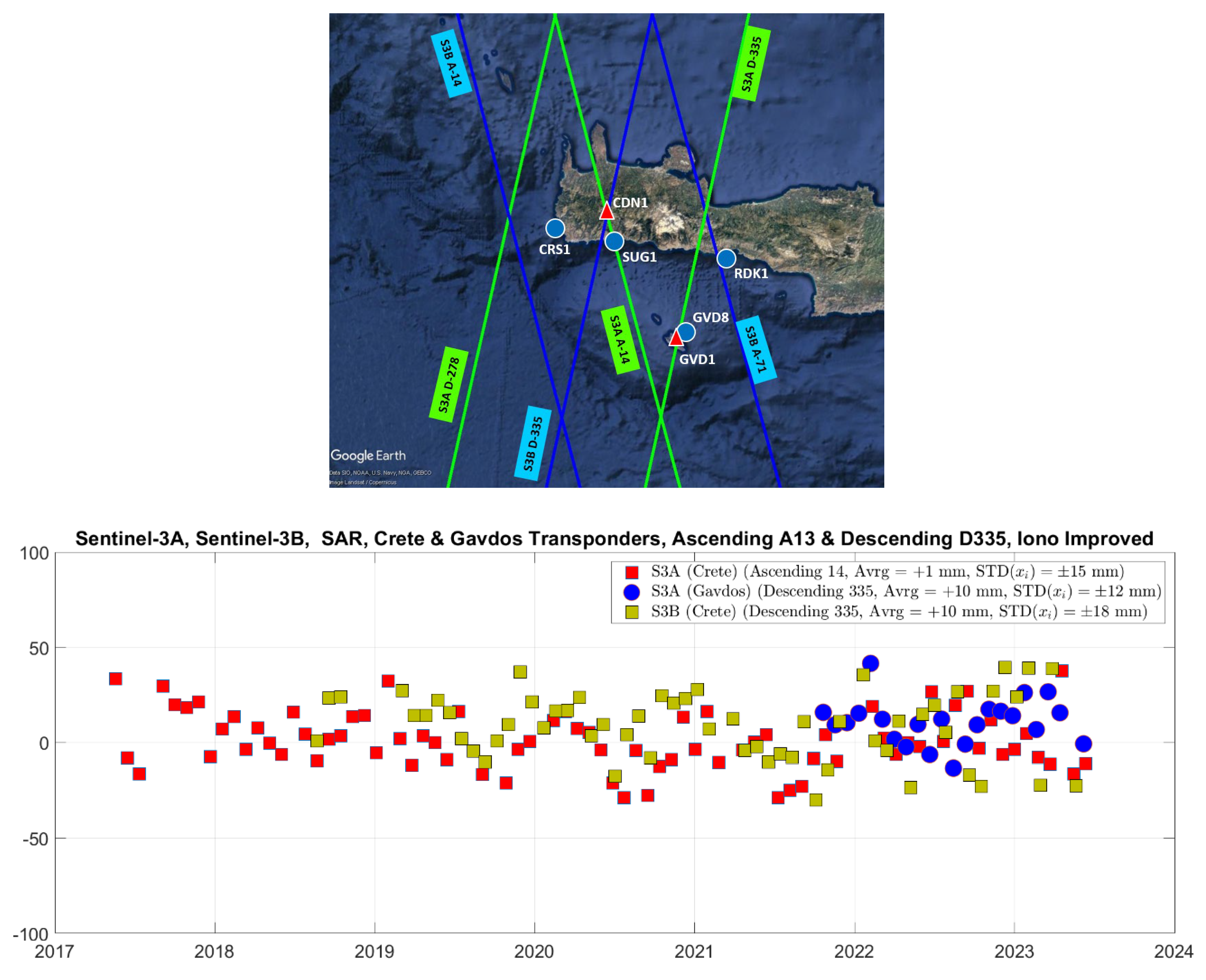
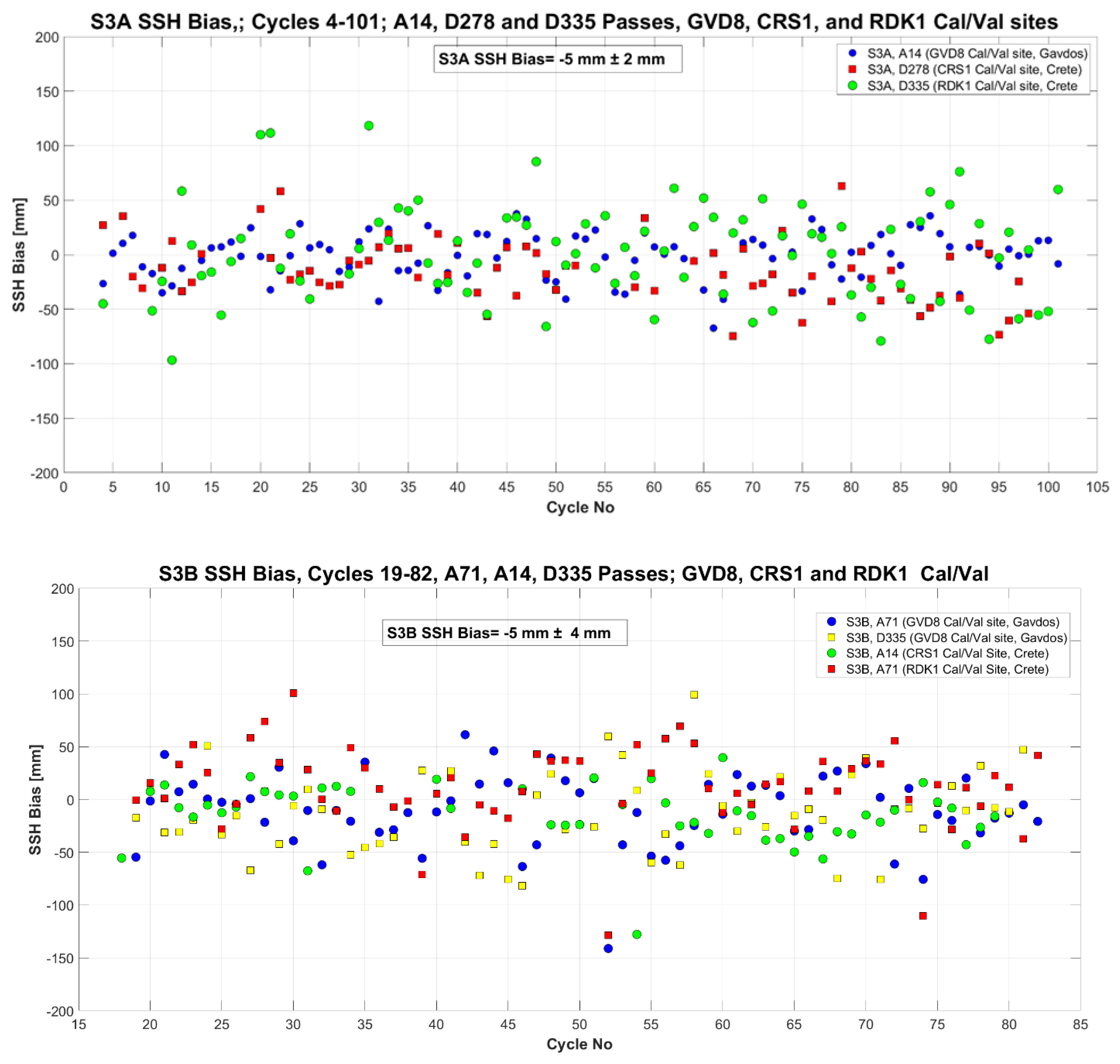
4.4. Sentinel-3 Sea-Surface Cal/Val Results

Figure 29 shows examples of the calibrating regions implemented for Sentinel-3A with the Gavdos and the CRS1 reference Cal/Val sites. Such ocean regions are over north and south zones around each site, where bathymetry is flat with minimal fluctuation in the dynamic topography and over locations with deep seas (i.e., bathymetry more than 2000 m). Similarly, Figure 30 shows Sentinel-3B examples of calibrating regions over the ocean and along its descending and ascending passes around the Gavdos and CRS1 Cal/Val sites. Two more sites, RDK1 and SUG1 in south Crete, have also been put into action in these sea-surface calibrations of Sentinel-3A/B.
In the PFAC, the determination of the final sea-surface height bias of Sentinel-3A and Sentinel-3B has been carried out by appropriate weighting of the results obtained per the Sentinel-3 cycle at each calibration site. Several factors were taken into consideration for delivering final results, such as the FRM uncertainty per site, percentage of missing tide gauge observations, dispersion of each independent time series, land contamination on altimetric measurements and products, etc.
Table 5 presents the sea-surface Cal/Val results for Sentinel-3A/B, as determined by the PFAC reference coastal sites in west and south Crete and Gavdos. The processing baseline PB 005.02 has been used for these results. In addition, Figure 31 presents the joined sea-surface Cal/Val results for both satellites from all Cal/Val sites together in one diagram. Each Cal/Val site produces its own bias, depending on the Cal/Val location used as a reference, the uncertainty of the selected reference surface (see also Section 3.5), the satellite ground track, and its associated bathymetry and geoid undulations.
Using both ascending and descending orbits and three Cal/Val sites, GVD8, CRS1, and RDK1, the aggregate average of SSH bias for Sentinel-3A comes to be B S 3 A ; G V D 8 , C R S 1 , R D K 1 = 7   mm   ±   2   mm , with an FRM uncertainty of u ( F R M ; S S H ) = ± 50   m m . In the same manner, Sentinel-3B calibrations deliver a sea-surface height bias of B S 3 B ; G V D 8 , C R S 1 , R D K 1 = 4   mm   ±   4   mm with the same FRM uncertainty. It can be observed in Figure 31 that the values of S3B are noisier than those of S3A. These results are in line with the ones derived by transponder calibrations.

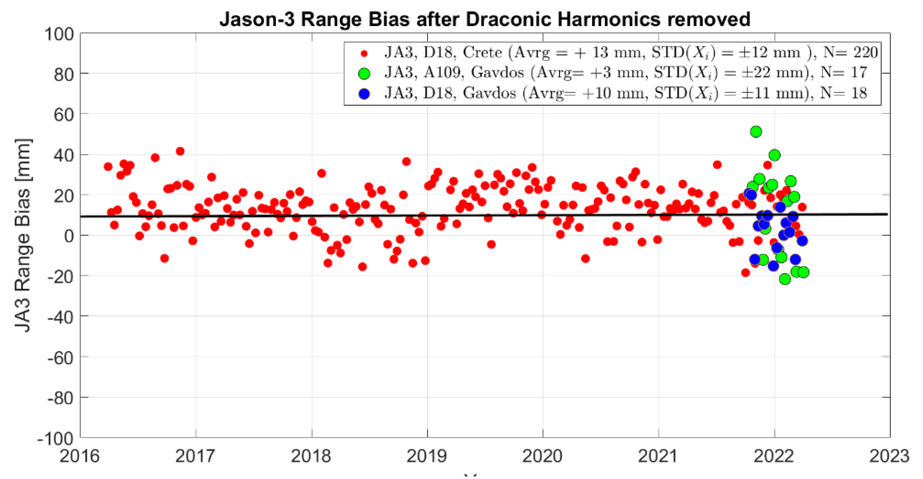
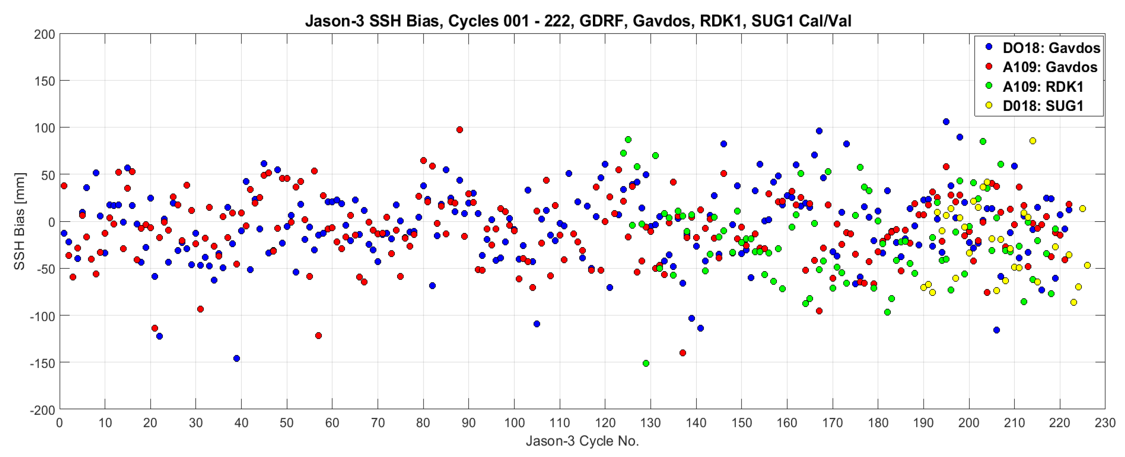
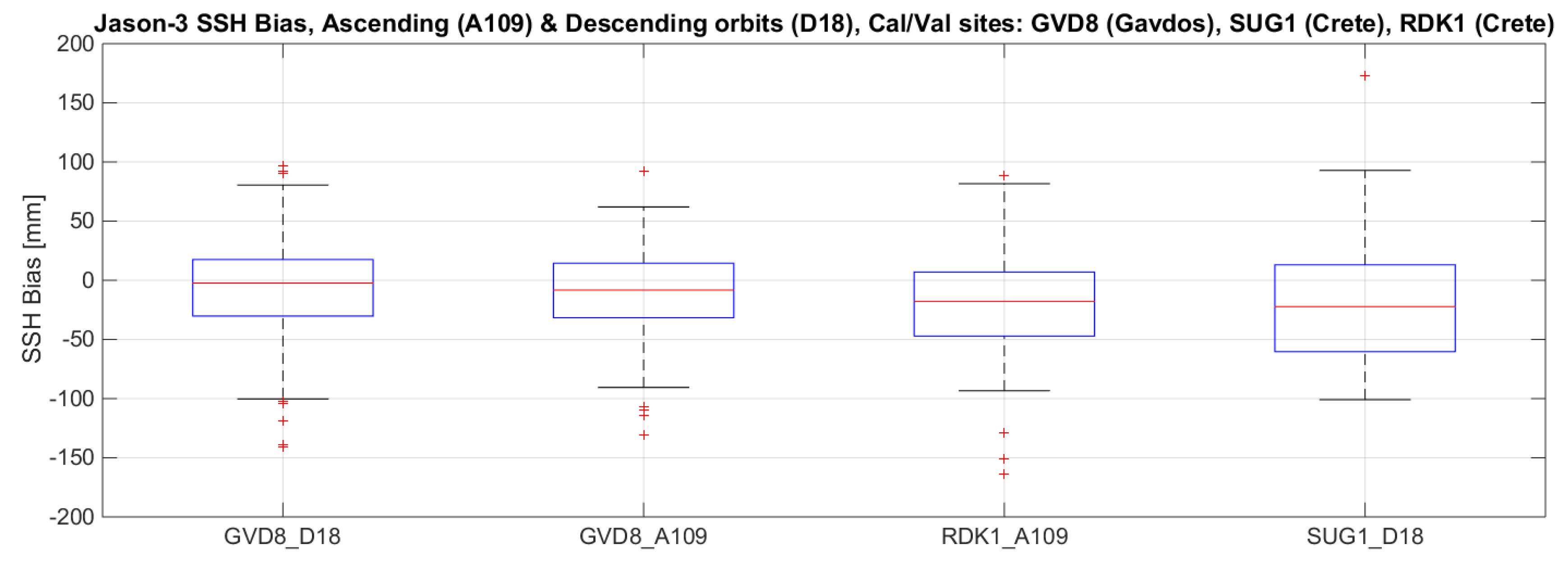
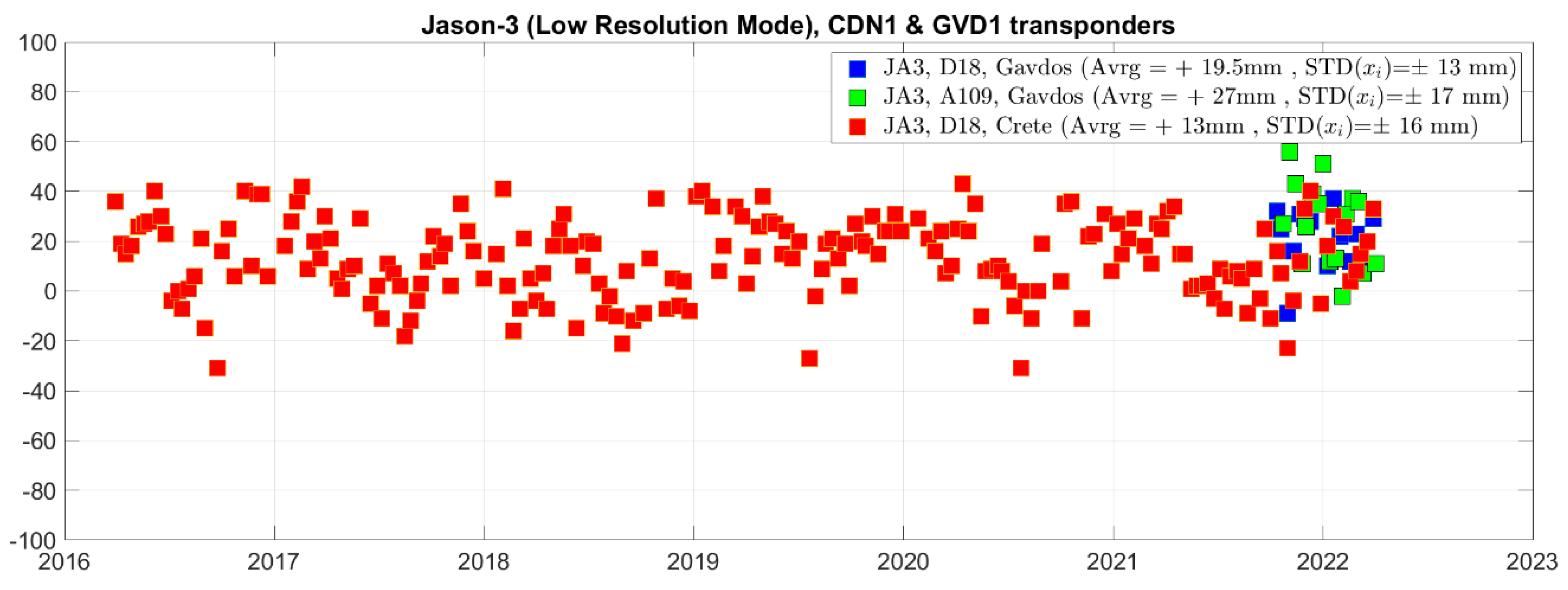
4.5. Jason-3 Cal/Val Results

After the successful launch of Jason-3 in January 2016 and during its Commissioning and Operational phases, the CDN1 transponder provided the capability to monitor its performance and continuously provided its absolute range bias for its Poseidon-3 altimeter. Also, the second transponder in Gavdos (operational as of 11 October 2021) and the additional SUG1 sea-surface Cal/Val site have built confidence in the estimations for the Jason-3 bias. Results are validated and have been cross-examined by diverse calibrations and ground infrastructures at different locations and settings.
Figure 32 presents the range bias for Jason-3 using the Crete and the Gavdos transponders. Oscillations are clear and primarily shown by the red squares in Figure 32 for the Crete transponder as this time series is long and contains 220 values (about 6 years). Such variations are predominately caused by the Draconic harmonics, which have not been removed in this case to demonstrate the effect. Respectively, fluctuations are not clearly obvious in the Gavdos data as they are only about 6 months long.
Figure 32 also shows that the average value for the bias of Jason-3 turns up with larger magnitudes at the Gavdos transponder (blue squares with B G V D 1 ; D 18 = + 19   mm , and green squares in Figure 28 with B G V D 1 ; A 109 = + 27   mm ) than the Crete transponder, i.e., B C D N 1 ; D 18 = + 13   mm . This is justified because Gavdos results correspond to an extent of time in which values of range bias commonly present a larger magnitude than the rest because of the Draconic oscillations. For instance, larger values of bias come into sight during winters and smaller values during summers. The Gavdos biases have been determined over winter months (October 2021–March 2022).
Subsequently, the Draconic harmonics were removed from the range bias for both the Crete and Gavdos transponders. Results are shown in Figure 33, after Draconic harmonics removal. The 6 years of range bias of Jason-3 using the Crete transponder produce an average value of B C D N 1 ; D 18 , J A 3 = + 13   mm   ±   12   mm   ,   ( N = 220 ) , while the Gavdos transponder gives an average of B G V D 1 ; J A 3 , D 18 = + 10   mm   ±   11   mm   ,   ( N = 17 ) for the descending and B G V D 1 ; J A 3 , A 109 = + 3   mm   ±   22   mm   ,   ( N = 18 ) for the ascending orbit. Jason-3 results are reasonable for both transponders. A small difference between biases along the ascending and descending orbits is evident in the Gavdos results of the order of a few mm (i.e., 7 mm in this case).
Sea-surface calibration for Jason-3 has also been carried out using its GDR-F products. Figure 34 shows these sea-surface Cal/Val results using the reference sites of Gavdos, SUG1 and RDK1 in south Crete and Gavdos (GVD8) along ascending and descending orbits. Also, in the lower diagram of Figure 34, boxplots concisely show these results.
In summary, Table 6 presents the complete calibration results for Jason-3 with the transponders and the sea-surface Cal/Val ground infrastructure. The uncertainty reported next to the average value corresponds to the sample standard deviation of the average, and not that of the FRM uncertainty. The FRM uncertainty for the Cal/Val results in the sea surface is ±46 mm and for the transponder Cal/Val results it is ±32 mm.

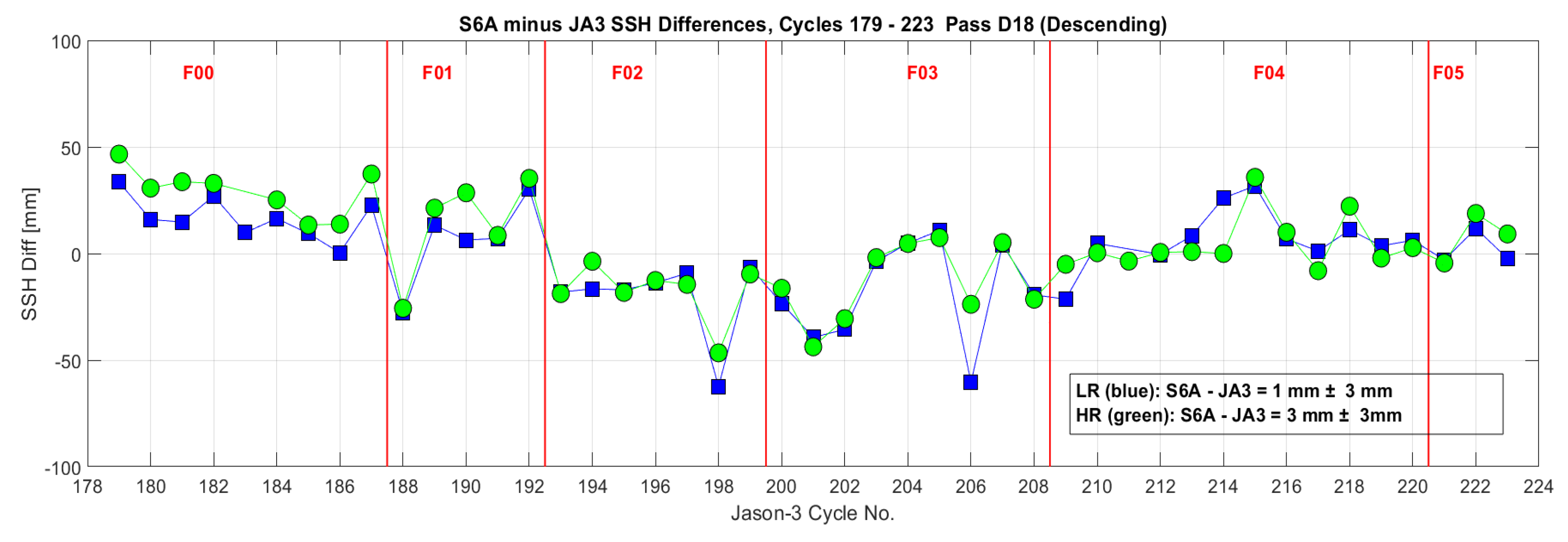
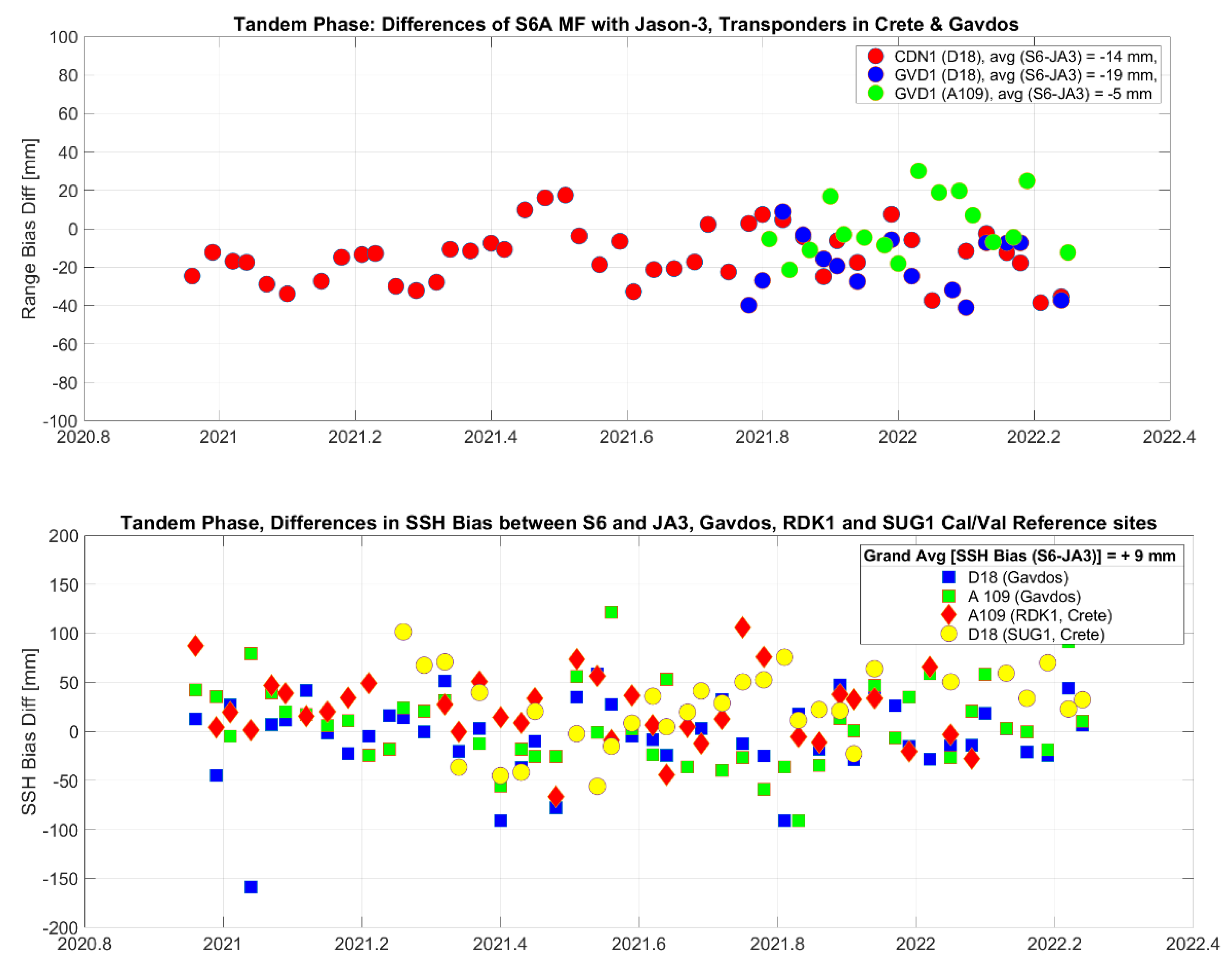
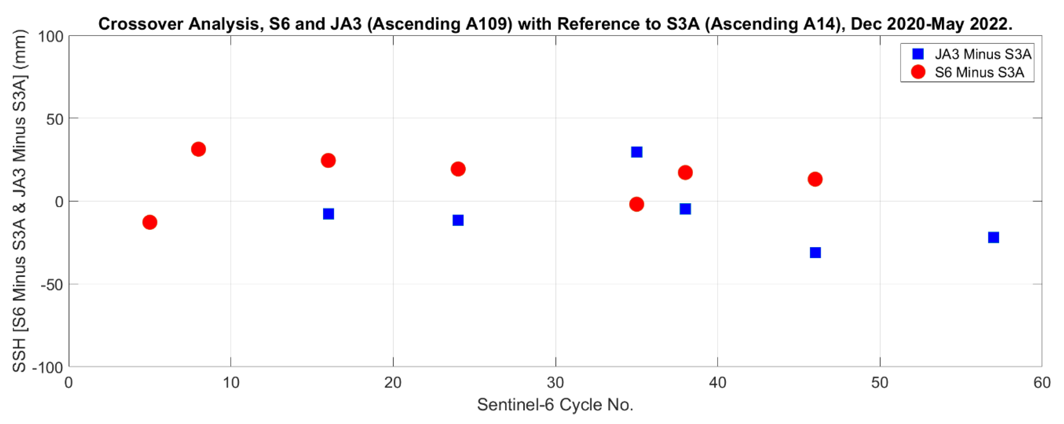
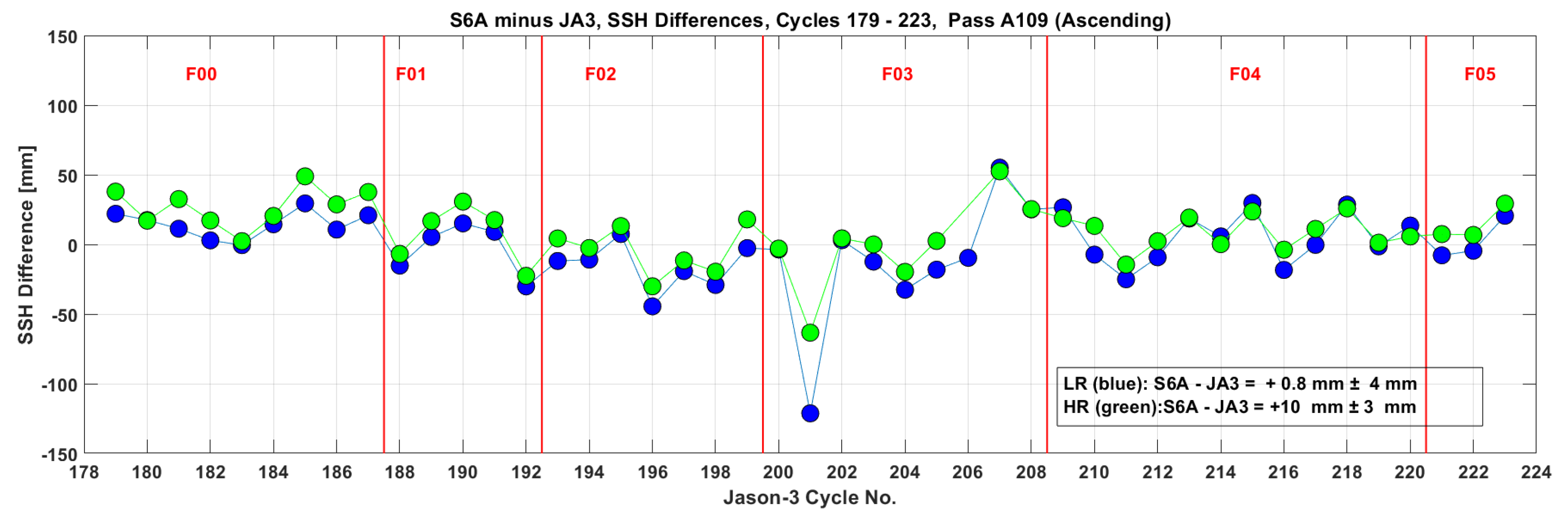
4.6. Jason-3 in Tandem with Sentinel-6 MF Cal/Val Results

To achieve a smooth transition of observations between missions and connect the old reference altimeter of Jason-3 with the new one of Sentinel-6 MF, a thorough evaluation of their relative performance had to be carried out during their tandem phase. The tandem formation lasted about 12 months, from 18 December 2020 to March 2022, and satellites were flying 220 km apart in the same orbit (~30 s). After the end of the tandem phase on 7 April 2022, Sentinel-6 MF was confirmed as the Reference Altimetry Mission. Comparisons between satellites were made with the transponders and the sea-surface Cal/Val infrastructure of the PFAC.
The upper diagram of Figure 35 presents the range bias difference of Sentinel-6 MF and Jason-3 using both transponders, at the CDN1 in Crete and GVD1 in Gavdos Cal/Val sites. The harmonic oscillations shown in both transponders in range difference indicate the Jason-3 yaw rotations towards the Sun [44]. An estimate of all these transponder calibrations during the tandem phase gives an average value of S 6 J A 3 = 12   mm   ±   1   mm ,   ( N = 83 ) , with 17 sample values along each ascending and descending orbit from Gavdos and 48 values from the CDN1 transponder in Crete.
The lower diagram of Figure 35 presents the SSH differences of both satellites with the sea-surface calibration, referenced to the GVD8 (Gavdos), SUG1, and RDK1 Cal/Val sites during their tandem phase. The aggregate average of all these differences in sea-surface heights from all Cal/Val sites provides an average value of S S H S 6 J A 3 = + 9   mm   ±   5   mm ,   ( N = 163 ) . The uncertainties next to the average values represent the sample standard deviation of the average, σ ( x j ¯ ) = ±   5   mm , while a realistic estimate of the FRM uncertainty is of u(FRM) = ±46 mm.

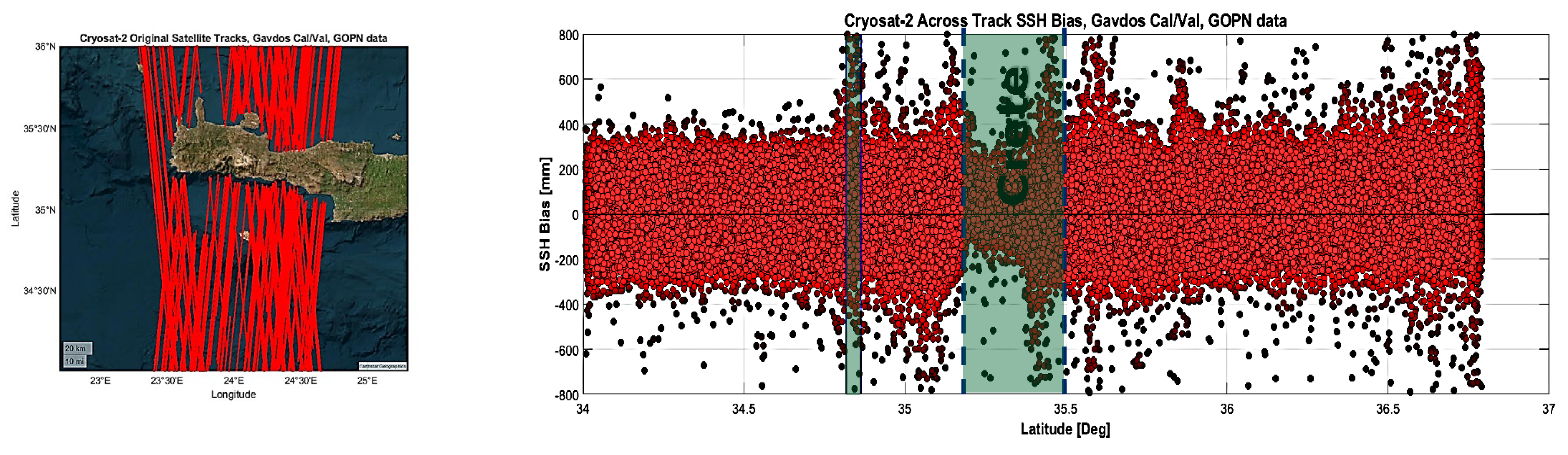
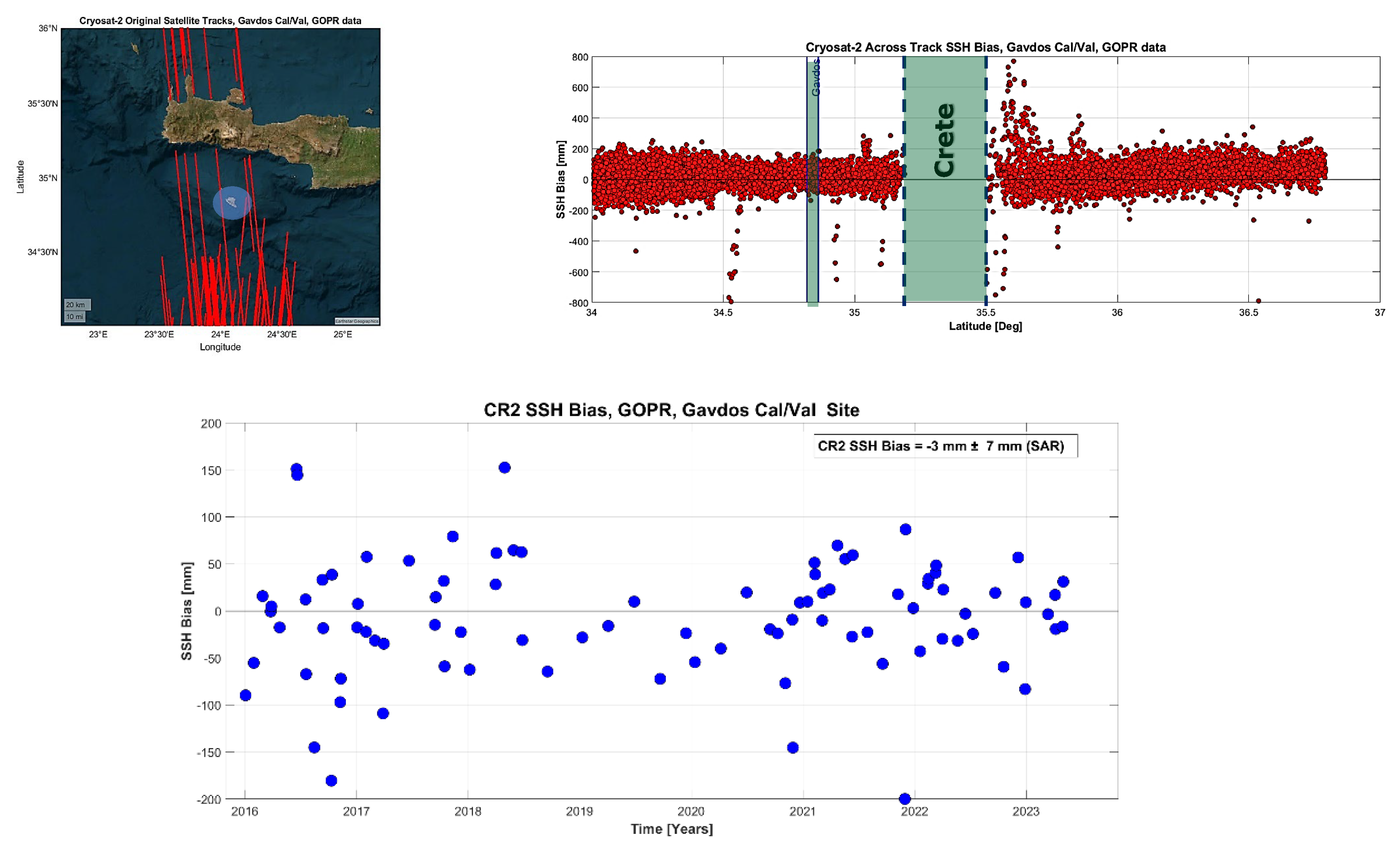
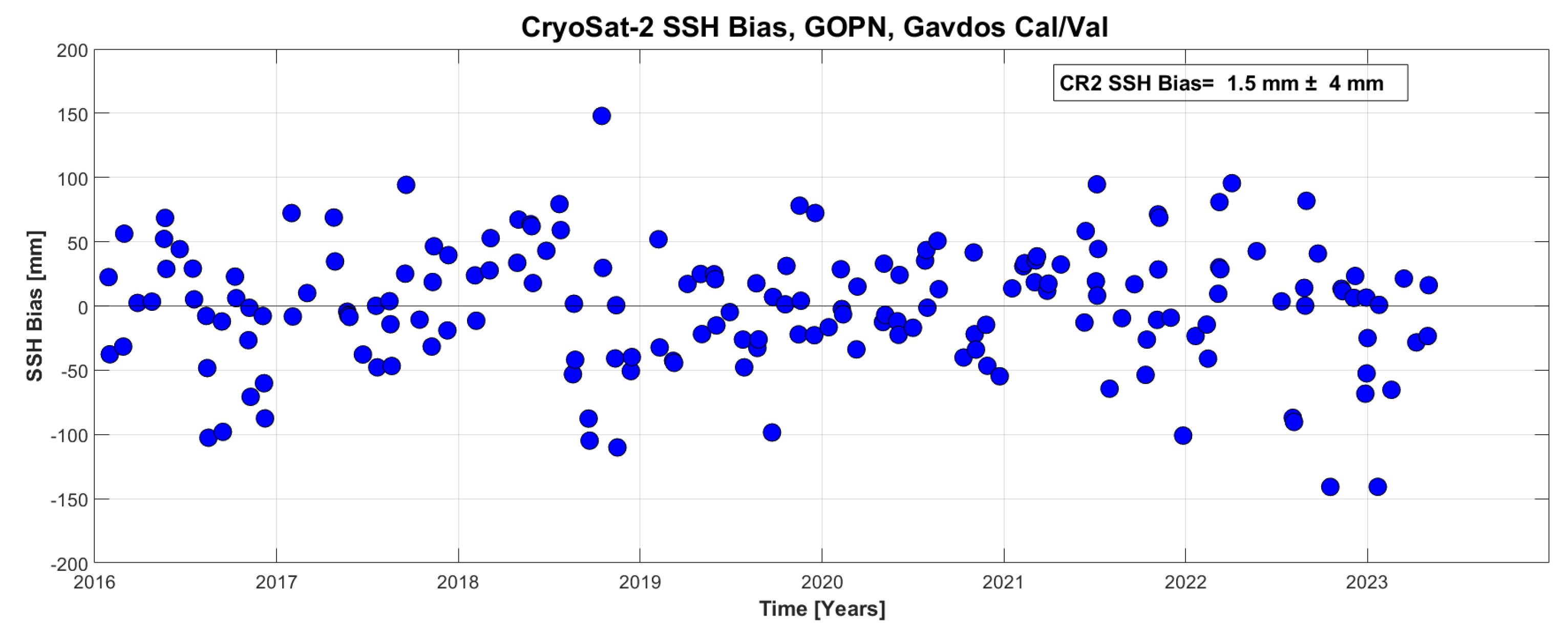
4.7. CryoSat-2 Sea-Surface Cal/Val Results

The PFAC has been supporting the calibration of the CryoSat-2 satellite from 2015 till today using its ground reference infrastructure, primarily with the sea-surface Cal/Val sites and with the transponders as well. Both the SAR and the SAR interferometry observations from the CryoSat-2 Geophysical Ocean Products (GOPs), Baseline C, have been used in this work [45]. Figure 36 shows the ground tracks of the SAR mode of Cryosat-2 (GOPR product) and the variations in the sea-surface height as a function of latitude. It also depicts the SSH bias of B C S 2 ; S A R = 3   mm   ±   7   mm for this set of SAR data from 2015 till the present (2023). Missing ground tracks in the GOP product indicate transponder calibrations taking place for which the altimeter range window is fixed around the exact transponder elevation. A certain number of seconds is required to switch between transponder and science mode for the altimeter onboard tracking system to look again on the sea surface.
In addition, Figure 37 shows similar results for the SARIn interferometric data (i.e., GOPN product) of CryoSat-2, covering again the same period of calibrations and using the same Gavdos Cal/Val site as a reference. As expected, the SARIn data are noisier than the SAR due to SARIn’s lower Burst Repetition Frequency [46,47], but Cal/Val results are numerous, giving an SHH bias of B C S 2 ; S A R I n = 1.5   mm   ±   4   mm ; keep in mind that the FRM uncertainty is u ( F R M ) =   ±   50   mm . Both results, in Figure 36 and Figure 37, refer to GOP Baseline-C products.

4.8. Crossover Analysis over the Sea Surface

The previous Cal/Val analyses required ground reference measurements provided by the PFAC infrastructure (i.e., transponders, tide gauges, GNSS, radiometers, meteorological sensors, gravimeters, etc.) along with modeling of geophysical parameters, such as the solid Earth displacement, mean dynamic topography, geoid undulation, etc.
Various observations generated by one satellite altimeter could be compared against another, whenever different orbits happened to converge at a common point in the ocean and within a short time interval [48]. To evaluate, thus, the relative performance of Sentinel-6 MF against Sentinel-3A, a location south of Gavdos was selected, where the descending Pass D18 of Sentinel-6 MF (and subsequently of Jason-3) and the ascending Pass A14 of Sentinel-3A intersected. Such a crossover point is shown in Figure 38. The procedure for applying a crossover analysis requires the following steps:
  • Single out passes of those satellites under examination, which converge at a sea location and contain a similar sea state and conditions; the last requirement is achieved by constraining the temporal difference of observations to be less than two days (48 h);
  • Interpolate neighboring altimeter data to estimate observations at the sought location of the crossover location;
  • Determine the geodetic coordinates of the crossover, as in general, it happens to be a point lying not exactly at the typical sequence of satellite observations (i.e., about 300 m, when 20 Hz sampling is used), but somewhere in between them;
  • Calculate the sea-surface heights at the crossover location for each altimeter, using a two-dimensional fitting of the original observations, and within a water stripe of 8 km on either side of the actual ground track;
  • Compare the two satellite altimeter observations and determine the relative bias at the crossover location.
During the Sentinel-6 MF and Jason-3 tandem phase, one would expect that the two missions would have the same crossover point with respect to Sentinel-3A. Nevertheless, this is not the case, because their offset distance was about 400 m (Figure 39).
The results of this crossover analysis were applied over the period between December 2020 to May 2022. Only very few values could fulfill the requirement for a 2-day time difference. Although the sample is small, it can be seen that the trend is that the S6-MF SSH is always higher than the JA3 SSH with reference to S3A. The relative SSH biases between Sentinel-6 MF and Jason-3 with respect to Sentinel-3A are +5 mm ±3 mm and +10 mm ± 2 mm, respectively (Figure 39).
Using Sentinel-3A as the reference, the relative SSH bias between Sentinel-6 MF and Jason-3 (S6 MF minus Jason-3) is determined to be of the order of 19   mm if we consider only valid cycles of Sentinel-6 MF and Jason-3 (Cycles 16, 24, 35, 38 of Figure 40). Although this crossover analysis is a rough comparison based on only four cycles, the behavior of the Poseidon-4 altimeter with respect to its predecessor Poseidon-3B appears to agree with the previous transponder results (Figure 25, Figure 28, and Figure 36).

5. Concluding Remarks

This work has described the ground infrastructure of the PFAC in Crete and presented the latest Cal/Val results for Sentinel-6 MF, Sentinel-3A, Sentinel-3B, Jason-3, and CryoSat-2. The Cal/Val results for the Chinese altimeter of HY-2B have been presented elsewhere [40].
For Sentinel-6 MF, transponders provide an average range bias of −4 mm (Crete, N = 94) and −2 mm (Gavdos, N = 63) for SAR observations, and −11 mm (Crete, N = 75) and +10 mm (Gavdos, N = 43) for its pseudo-range observations. The corresponding sea-surface height bias of Sentinel-6 MF amounts to an average of −17 mm, based on three Cal/Val sites in Crete and Gavdos and using about N = 100 observations. Results are based on ascending and descending orbits with L1A data and precise orbits (Non-Time Critical) for the transponders and with the Processing Baseline F08 for the sea surface. Associated uncertainties are for the transponder ±30 mm, and ±45 mm for the sea-surface height results, in accordance with the principle of Fiducial Reference Measurements. Sentinel-3A and Sentinel-3B exhibit, respectively, an average range bias of +5 mm (Crete, N = 78 and Gavdos, N = 18) and +10 mm (Crete, N = 55), with biases of −7 mm and −4 mm in sea-surface heights. Jason-3 shows a range bias of +13 mm and a −11 mm bias in sea-surface heights, weighted by the number of observations. The CryoSat-2 bias comes to almost zero over 7 years of observations at sea.
All in all, such a facility provides Cal/Val services for all international altimeters and integrates various contributions coming from a combination of different sites, technologies, observations, and settings. Its ultimate goal has been to monitor reliably and confidently the performance of a satellite altimeter in the wake of the dramatic and quick developments in climate and sea level change.
The quality control employed for the reference observations and the baseline processing, as well as the way uncertainties are produced for each calibration, have also been outlined, be it the transponder or the sea-surface height calibration, following the recommendations of the FRM strategy of ESA and the Guide of Uncertainty Measurements prescribed by the International Bureau of Weights and Measures (Bureau International des Poids et Mesures, BIPM).
The new transponder facility on Gavdos Island was described and its characterization and field tests before final deployment have been given. The instrument redundancy of this new facility has been strengthened by the installation of a third GNSS station, part of the French network REGINA, while the old DORIS site has been again operational with a new generation beacon. As of 29 July 2023, a corner reflector, named ALX1 (Figure 40), has also been established in Crete for the calibration of Sentinel-6 MF, Sentinel-3A, and Sentinel-3B, while another one is ready to be deployed.
In summary, it can be stated that (1) based on the transponder and sea-surface calibrations at the ground facility of the PFAC and the available baseline processing, the Sentinel-6 MF, Sentinel-3A, Sentinel-3B, Jason-3, and CryoSat-2 altimetric observations are within each mission’s specifications; (2) the absolute uncertainty of these PFAC-derived results is of the order of ±2 cm for the transponder and ±4–5 cm for the sea-surface calibrations; (3) the asymmetry in the Sentinel-6 transponder waveforms exists in any other satellite waveform, but it could be only compensated for in Sentinel-6 because of its detailed shape reconstruction. The low resolution in Sentinel-3 waveforms, for example, does not allow such a rectification, and, thus, adjustment for its asymmetry. The same holds true for the pseudo-low-resolution mode; (4) waveform asymmetry is present because of the orientation of the antenna array of the transponder with respect to the satellite orbit.

Author Contributions

Conceptualization, S.P.M., A.T. and C.D.; methodology, S.P.M., A.T., C.K. and D.P.; software, C.K., D.P., A.T., S.P.M. and X.F.; validation, C.K., D.P., A.T., S.P.M. and X.F.; formal analysis, S.P.M., C.K., D.P., A.T. and X.F.; investigation, S.P.M., C.K., D.P., A.T. and X.F.; resources, S.P.M., C.D., C.K., D.P., A.T. and X.F.; data curation, S.P.M., C.K., D.P., A.T., F.B. and X.F.; writing—original draft preparation, S.P.M. and A.T.; writing—review and editing, S.P.M., P.F., R.C., M.F., J.B., A.D.B., J.S., A.T. and X.F.; visualization, S.P.M., C.K., D.P., A.T. and X.F.; supervision, S.P.M., C.D. and A.D.B.; project administration, S.P.M., C.D., P.F. and A.D.B.; funding acquisition, S.P.M. and C.D. All authors have read and agreed to the published version of the manuscript.

Funding

Τhis research was partially funded by the European Union and the European Space Agency (grant number 4000129892/20/NL/FF/ab). The help and support of Thomas Donal and Damien Pesce of the IGN (National Institute of Geographic and Forest Information), Paris, France, and Laurent Jolivet of CNES, Toulouse, France is greatly appreciated. This work has been supported by the European Space Agency through the FRM4S6 Project (4000129892/20/NL/FF/ab), the Mission Performance Cluster of Sentinel-3 (CLS, Toulouse, France) and the Project “Calibration of CryoSat’s Range and Interferometric Phase using Transponders” (4000111597/14/I-AM) (IsardSat, Catalonia).

Data Availability Statement

Sentinel-3 and Sentinel-6 products used for calibration processing are available from the centralized EUMETSAT site: https://data.eumetsat.int (accessed on 2 January 2024). CryoSat-2 products are available at https://eocat.esa.int/sec/#data-services-area/ (accessed on 2 January 2024) and https://earth.esa.int/eogateway/catalog/cryosat-products (accessed on 2 January 2024).

Conflicts of Interest

The authors declare no conflicts of interest.

References

  1. International Altimetry Team. Altimetry for the future: Building on 25 years of progress. Adv. Space Res. 2021, 68, 319–363. [Google Scholar] [CrossRef]
  2. Sterckx, S.; Brown, I.; Kääb, A.; Krol, M.; Morrow, R.; Veefkind, P.; Boersma, K.F.; De Mazière, M.; Fox, N.; Thorne, P. Towards a European Cal/Val service for earth observation. Int. J. Remote Sens. 2020, 41, 4496–4511. [Google Scholar] [CrossRef]
  3. Francis, C.R.; Caporali, A.; Cavaleri, L.; Cenci, A.; Ciotto, P.; Ciraolo, L.; Gurtner, W.; Massmann, F.H.; del Rosso, D.; Scharroo, R.; et al. The Calibration of the ERS-1 Radar Altimeter-The Venice Calibration Campaign; ESA Report ER-RP-ESA-RA-0257 Issue 2.0; ESA/ESTEC: Noordwijk, The Netherlands, 1993. [Google Scholar]
  4. Mondéjar, A.G.; Fornari, M.; Bouffard, J.; Féménias, P.; Roca, M. CryoSat-2 range, datation and interferometer calibration with Svalbard transponder. Adv. Space Res. 2008, 62, 1589–1609. [Google Scholar] [CrossRef]
  5. Haines, B.; Desai, S.D.; Kubitschek, D.; Leben, R.R. A brief history of the harvest experiment: 1989-2019. Adv. Space Res. 2020, 68, 1161–1170. [Google Scholar] [CrossRef]
  6. Bonnefond, P.; Exertier, P.; Laurain, O.; Guinle, T.; Féménias, P. Corsica: A 20-Yr multi-mission absolute altimeter calibration site. Adv. Space Res. 2020, 68, 1171–1186. [Google Scholar] [CrossRef]
  7. Watson, C.; White, N.; Church, J.; Burgette, R.; Tregoring, P.; Coleman, R. Absolute Calibration in Bass Strait, Australia: TOPEX, Jason-1 and OSTM/Jason-2. Mar. Geod. 2011, 34, 242–260. [Google Scholar] [CrossRef]
  8. Mertikas, S.P.; Donlon, C.; Féménias, P.; Mavrocordatos, C.; Galanakis, D.; Tripolitsiotis, A.; Frantzis, X.; Tziavos, I.N.; Vergos, G.; Guinle, T. Fifteen Years of Cal/Val Service to Reference Altimetry Missions: Calibration of Satellite Altimetry at the Permanent Facilities in Gavdos and Crete, Greece. Remote Sens. 2018, 10, 1557. [Google Scholar] [CrossRef]
  9. Chen, C.; Zhu, J.; Ma, C.; Lin, M.; Yan, L.; Huang, X.; Zhai, W.; Mu, B.; Jia, Y. Preliminary calibration results of the HY-2B altimeter’s SSH at China’s Wanshan calibration site. Acta Oceanol. Sin. 2021, 40, 129–140. [Google Scholar] [CrossRef]
  10. Yang, L.; Xu, Y.; Zhou, X.; Zhu, L.; Jiang, Q.; Sun, H.; Chen, G.; Wang, P.; Mertikas, S.P.; Fu, Y.; et al. Calibration of an Airborne Interferometric Radar Altimeter over the Qingdao Coast Sea, China. Remote Sens. 2020, 12, 1651. [Google Scholar] [CrossRef]
  11. Morrow, R.; Fu, L.-L.; Ardhuin, F.; Benkiran, M.; Chapron, B.; Cosme, E.; d’Ovidio, F.; Farrar, J.T.; Gille, S.T.; Lapeyre, G.; et al. Global Observations of Fine-Scale Ocean Surface Topography with the Surface Water and Ocean Topography (SWOT) Mission. Front. Mar. Sci. 2019, 6, 232. [Google Scholar] [CrossRef]
  12. Chupin, C.; Ballu, V.; Testut, L.; Tranchant, Y.-T.; Aucan, J. Noumea: A new multi-mission Cal/Val site for past and future altimetry missions? EGUsphere 2022, 2022, 1–37. [Google Scholar] [CrossRef]
  13. Donlon, C.; Berruti, B.; Buongiorno, A.; Ferreir, M.-H.; Féménias, P.; Frerick, J.; Goryl, P.; Klein, U.; Laur, H.; Mavrocordatos, C.; et al. The Global Monitoring for Environment and Security (GMES) Sentinel-3 mission. Remote Sens. Environ. 2012, 120, 37–57. [Google Scholar] [CrossRef]
  14. Parkinson, C.L. Satellite Contributions to Climate Change Studies. Proc. Am. Philos. Soc. 2017, 161, 208–225. [Google Scholar]
  15. Mertikas, S.P.; Tripolitsiotis, A.; Donlon, C.; Mavrocordatos, C.; Féménias, P.; Borde, F.; Frantzis, X.; Kokolakis, C.; Guinle, T.; Vergos, G.; et al. The ESA Permanent Facility for Altimetry Calibration: Monitoring Performance of Radar Altimeters for Sentinel-3A, Sentinel-3B and Jason-3 using Transponder and Sea-Surface Calibrations with FRM Standards. Remote Sens. 2020, 12, 2642. [Google Scholar] [CrossRef]
  16. Mertikas, S.P.; Donlon, C.; Vuilleumier, P.; Cullen, R.; Féménias, P.; Tripolitsiotis, A. An Action Plan towards Fiducial Reference Measurements for Satellite Altimetry. Remote Sens. 2019, 11, 1993. [Google Scholar] [CrossRef]
  17. Goryl, P.; Fox, N.; Donlon, C.; Castracane, P. Fiducial Reference Measurements (FRMs): What Are They? Remote Sens. 2023, 15, 5017. [Google Scholar] [CrossRef]
  18. Rodriguez, E.; Fernandez, D.E.; Peral, E.; Chen, C.W.; De Bleser, J.-W.; Williams, B. Wide Swath Altimetry: A Review. In Satellite Altimetry over Oceans and Lakes, 1st ed.; Stammer, D., Cazenave, A., Eds.; CRC Press: Boca Raton, FL, USA, 2017; pp. 71–113. [Google Scholar] [CrossRef]
  19. Verron, J.; Bonnefond, P.; Aouf, L.; Birol, F.; Bhowrnic, S.; Calmant, S.; Conchy, T.; Crétaux, J.-F.; Dibarboure, G.; Dubey, A.K.; et al. The benefits of the Ka-band as evidenced from the SARAL/Altika altimetric mission: Sci-entific Applications. Remote Sens. 2018, 10, 163. [Google Scholar] [CrossRef]
  20. Myasoedov, A.; Johannessen, J.A.; Kudryavtsev, V.; Collard, F.; Chapron, B. Sun glitter as a “tool” for monitoring Ocean from Space. In Proceedings of the 2nd International Conference on Remote Sensing, Enviornment and Transportation Engineering, Nanjing, China, 1–3 June 2012. [Google Scholar] [CrossRef]
  21. Roesler, C.; Larson, K.M. Software tools for GNSS interferometric reflectometry (GNSS-IR). GPS Solut. 2018, 22, 80. [Google Scholar] [CrossRef]
  22. Zheng, N.; Chai, H.; Ma, Y.; Chen, L.; Chen, P. Hourly sea level height forecast based on GNSS-IR using ARIMA model. Int. J. Remote Sens. 2022, 43, 3387–3411. [Google Scholar] [CrossRef]
  23. Chen, C.; Desai, S.; Picot, N.; Fu, L.-L.; Morrow, R.; Pavelsky, T.; Cretaux, J.-F. SWOT Calibration/Validation Plan. 2018. Available online: https://swot.jpl.nasa.gov/system/documents/files/2244_2244_D-75724_SWOT_Cal_Val_Plan_Initial_20180129u.pdf (accessed on 5 August 2022).
  24. Mertikas, S.P.; Partsinevelos, P.; Tripolitsiotis, A.; Kokolakis, C.; Petrakis, G.; Frantzis, X. Validation of Sentinel-3 OLCI In-tegrated Water Vapor Products using regional GNSS measurements in Crete, Greece. Remote Sens. 2020, 12, 2606. [Google Scholar] [CrossRef]
  25. Donlon, C.; Cullen, R.; Giulicchi, L.; Vuilleumier, P.; Francis, R.C.; Kuschnerus, M.; Simpson, W.; Bouridah, A.; Caleno, M.; Bertoni, R.; et al. The Copernicus Sentinel-6 mission: Enhanced continuity of satellite sea level measurements from space. Remote Sens. Environ. 2021, 258, 112395. [Google Scholar] [CrossRef]
  26. Giulicchi, I.; Tavernier, G.; Picot, N.; Cullen, R.; Scharroo, R.; Martin-Puig, C.; Desai, S.; Desjonquerres, J.D.; Leuliette, E.; Egido, A. Sentinel-6/Jason-CS Cal/Val Concept; JC-PL-ESA-MI-0500; European Space Research and Technology Centre: Noordwijk, The Netherlands, 2019; Available online: https://shorturl.at/jLWZ6 (accessed on 8 August 2023).
  27. Willis, P.; Mertikas, S.P.; Argus, D.F.; Bock, O. DORIS and GPS monitoring of the Gavdos calibration site in Crete. Adv. Space Res. 2013, 51, 1438–1447. [Google Scholar] [CrossRef]
  28. Herring, T.A.; King, R.W.; McClusky, S.C. GAMIT Reference Manual: GPS Analysis at MIT, Release 10.7; Massachusetts Institute of Technology: Cambridge, MA, USA, 2020. [Google Scholar]
  29. Collins, P.; Bisnath, S.; Lahaye, F.; Heroux, P. Undifferenced GPS ambiguity resolution using the decoupled clock model and ambiguity datum fixing. Navigation 2010, 57, 123–135. [Google Scholar] [CrossRef]
  30. Mertikas, S.P.; Donlon, C.; Mavrocordatos, C.; Piretzidis, D.; Kokolakis, C.; Cullen, R.; Matsakis, D.; Borde, F.; Fornari, M.; Boy, F.; et al. Performance evaluation of the CDN1 altimetry Cal/Val transponder to internal and external constituents of uncertainty. Adv. Space Res. 2022, 70, 2458–2479. [Google Scholar] [CrossRef]
  31. Miguez Martin, B.; Testut, L.; Woppelmann, G. Performance of modern tide gauges: Towards mm-level accuracy. Sci. Mar. 2012, 76, 221–228. [Google Scholar] [CrossRef]
  32. Gorbon, K.; de Viron, O.; Wöppelmann, G.; Poirier, É.; Ballu, V.; Van Camp, M. Assessment of tide gauge biases and precision by the combination of multiple collocated time series. J. Atmos. Ocean. Technol. 2019, 36, 1983–1996. [Google Scholar] [CrossRef]
  33. Miguez Martin, B.; Testut, L.; Woppelmann, G. The van de Casteele test revisited: An efficient approach to tide gauge error characterization. J. Atmos. Ocean. Technol. 2008, 25, 1238–1244. [Google Scholar] [CrossRef]
  34. Mertikas, S.P. Description of accuracy using conventional and robust estimates of scale. Mar. Geod. 1994, 17, 251–269. [Google Scholar] [CrossRef]
  35. Zingerle, P.; Pail, R.; Gruber, T.; Oikonomidou, X. The combined global gravity field model XGM2019e. J. Geod. 2020, 94, 66. [Google Scholar] [CrossRef]
  36. Förste, C.; Bruinsma, S.; Flechtner, F.; Abrykosov, O.; Dahle, C.; Marty, J.; Lemoine, J.; Biancale, R.; Barthelmes, F.; Neumayer, K.; et al. EIGEN-6C4 the latest combined global gravity field model including GOCE data up to degree and order 2190 of GFZ Potsdam and GRGS Toulouse. In GFZ Data Services; GFZ German Research Centre for Geosciences: Potsdam, Germany, 2014. [Google Scholar] [CrossRef]
  37. Gilardoni, M.; Reguzzoni, M.; Sampietro, D. GECO: A global gravity model by locally combining GOCE data and EGM2008. Stud. Geophys. Geod. 2016, 60, 228–247. [Google Scholar] [CrossRef]
  38. Thibaut, P.; Piras, F.; Roinard, H.; Guerou, A.; Boy, F.; Maraldi, C.; Bignalet-Cazalet, F.; Dibarboure, G.; Picot, N. Benefits of the adaptive retracking solution for the Jason-3 GDR-F reprocessing campaign. In Proceedings of the 2021 IEEE International Geoscience and Remote Sensing Symposium, Brussels, Belgium, 11–16 July 2021; pp. 7422–7425. [Google Scholar] [CrossRef]
  39. Mertikas, S.P.; Donlon, C.; Féménias, P.; Cullen, R.; Galanakis, D.; Frantzis, X.; Tripolitsiotis, A. Fiducial Reference Measurements for Satellite Altimetry Calibration: The Constituents. In Fiducial Reference Measurements for Altimetry; Mertikas, S., Pail, R., Eds.; International Association of Geodesy Symposia; Springer: Cham, Switzerland, 2019; Volume 150, pp. 1–6. [Google Scholar] [CrossRef]
  40. Mertikas, S.P.; Lin, M.; Piretzidis, D.; Kokolakis, C.; Donlon, C.; Ma, C.; Zhang, Y.; Jia, Y.; Mu, B.; Frantzis, X.; et al. Absolute Calibration of the Chinese HY-2B Altimetric Mission with Fiducial Reference Measurement Standards. Remote Sens. 2023, 15, 1393. [Google Scholar] [CrossRef]
  41. Andersen, O.B.; Zhang, S.; Sandwell, D.T.; Dibarboure, G.; Smith, W.H.F.; Abulatijiang, A. The Unique Role of the Jason Ge-odetic Missions for high Resolution Gravity Field and Mean Sea Surface Modelling. Remote Sens. 2021, 13, 646. [Google Scholar] [CrossRef]
  42. Cullen, R.; Donlon, C.; Fornari, M.; Giulicchi, L. Sentinel-6 Michael Freilich Poseidon-4 Altimeter In-Orbit Performance. In Proceedings of the GARSS 2022-2022 IEEE International Geoscience and Remote Sensing Symposium, IEEE, Kuala Lumpur, Malaysia, 17–22 July 2022; pp. 6791–6794. [Google Scholar] [CrossRef]
  43. Mertikas, S.P.; Daskalakis, A.; Tziavos, I.N.; Andersen, O.B.; Vergos, G.; Tripolitsiotis, A.; Zervakis, V.; Frantzis, X.; Partsinevelos, P. Altimetry, bathymetry and geoid variations at the Gavdos permanent Cal/Val facility. Adv. Space Res. 2013, 51, 1418–1437. [Google Scholar] [CrossRef]
  44. Kokolakis, C.; Piretzidis, D.; Mertikas, S.P. Impact of Satellite Attitude on Altimetry Calibration with Microwave Transponders. Remote Sens. 2022, 14, 6369. [Google Scholar] [CrossRef]
  45. Naeije, M.; Di Bella, A.; Geminale, T.; Visser, P. CryoSat Long-Term Ocean Data Analysis and Validation: Final Words on GOP Baseline-C. Remote Sens. 2023, 15, 5420. [Google Scholar] [CrossRef]
  46. Windham, D.J.; Francis, C.R.; Baker, S.; Bouzinac, C.; Brockley, D.; Cullen, R.; de Chateau-Thierry, P.; Laxon, S.W.; Mallow, U.; Mavrocordatos, C.; et al. CryoSat: A mission to determine the fluctuations in Earth’s land and marine ice fields. Adv. Space Res. 2006, 37, 841–871. [Google Scholar] [CrossRef]
  47. Di Bella, A.; Kwok, R.; Armitage, T.W.K.; Skourup, H.; Forsberg, R. Multi-peak Retracking of CryoSat-2 SARIn Waveforms Over Arctic Sea Ice. IEEE Trans. Geosci. Remote Sens. 2021, 59, 3776–3792. [Google Scholar] [CrossRef]
  48. Dettmering, D.; Schwatke, C. Multi-Mission Cross-Calibration of Satellite Altimeters. In Fiducial Reference Measurements for Altimetry; Mertikas, S.P., Pail., R., Eds.; Springer International Publishing: Berlin/Heidelberg, Germany, 2020; pp. 49–54. [Google Scholar] [CrossRef]
Figure 1. The reference ground sites for altimetry calibration that constitute the European Space Agency PFAC with two transponder (CDN1, GVD1) and four sea-surface (GVD8, CRS1, RDK1, SUG1) Cal/Val sites. The ground tracks of Sentinel-6 MF/Jason-3, Sentinel-3A/B, HY-2B satellite altimetry missions over Crete, Greece are also shown. CryoSat-2 ground tracks (same as CRISTAL) are not shown in this figure but some of its orbits are given in Section 4.7.
Remotesensing 16 00223 g001
Figure 2. The CDN1 range transponder at the calibration site, in the mountains of west Crete at 1050 m elevation.
Remotesensing 16 00223 g002
Figure 3. (Left) The CDN1 transponder buried deep in snow. Over winters, harsh conditions prohibit satellite calibration with the CDN1 transponder. (Right) The assessment of the performance of the CDN1 transponder calibrations in the period 1 October 2015 to September 2023. The numbers inside the bars indicate the number of successful and cancelled calibrations.
Remotesensing 16 00223 g003
Figure 4. The location of the GVD1 Cal/Val site is ideal for Sentinel-6 MF calibrations as it lies under a crossover of its descending Pass No. 18 and its ascending Pass No. 109.
Remotesensing 16 00223 g004
Figure 5. Two transponder Cal/Val sites (GVD1 and CDN1) and two sea-surface Cal/Val facilities (GVD8 in Gavdos and SUG1 in Crete) support calibration of Sentinel-6 MF Pass D18.
Remotesensing 16 00223 g005
Figure 6. Records of output signal of the ELECTRA transponder during the Sentinel-6 MF and Jason-3 tandem calibration on 7 February 2022 for their common descending Pass No. 18.
Remotesensing 16 00223 g006
Figure 7. The primary design components of the ELECTRA transponder (left) and final setting of the infrastructure on Gavdos Island (right).
Remotesensing 16 00223 g007
Figure 8. Tests of the transponder carried out at ESTEC/ESA in The Netherlands (left) and in Athens, Greece (right).
Remotesensing 16 00223 g008
Figure 9. Field testing of the ELECTRA transponder before its shipment to Gavdos. Temporary site CRD1 was about 3 km west of the ascending pass No. 70 of Sentinel-3B on 23 July 2021 and of CryoSat-2 on 29 July 2021 in the mainland of Crete.
Remotesensing 16 00223 g009
Figure 10. Left: Transponder response as recorded on Sentinel-3B for the 23 July 2021 pass over the temporary CRD1 Cal/Val site. Right: the power of the RF transmitted signal as recorded by the ELECTRA transponder during the 29 July 2021 CryoSat-2 transponder calibration (transponder starts recording as the data is captured).
Remotesensing 16 00223 g010
Figure 11. The layout of the GVD1 Cal/Val site with the main outdoor scientific instrumentation (above) and the new DORIS antenna (GAVC) as well as the control room inside the calibration site in Gavdos (below).
Remotesensing 16 00223 g011
Figure 12. A small fishing harbor on the south coast of Crete was selected for the SUG1 Cal/Val site (left). Main scientific instrumentation operating since March 2021.
Remotesensing 16 00223 g012
Figure 13. Two GNSS receivers are continuously operating at each transponder Cal/Val site: CDN1 on the mainland of Crete (left) and GVD1, Gavdos Island (right).
Remotesensing 16 00223 g013
Figure 14. Time series of the GVD2 ellipsoidal height as calculated using the relative and precise point positioning.
Remotesensing 16 00223 g014
Figure 15. Differences in total tropospheric delays at the CDN0 and CDN2 GNSS stations, derived through relative positioning at the time of Sentinel–6 MF transponder calibrations.
Remotesensing 16 00223 g015
Figure 16. Differences in total tropospheric delays for the CDN0 GNSS station as estimated by relative and precise point positioning at the CDN1 transponder site during the Sentinel–6 MF calibrations (up). Boxplots of the two different analyses for the determination of the total troposphere delays (down).
Remotesensing 16 00223 g016
Figure 17. The location of the ELECTRA transponder on Gavdos Island and the ground tracks of Sentinel–6 MF (D18 and A109) and that of Sentinel–3A (D335) (a). The other two diagrams show the waveforms recorded by Sentinel–6 MF for the ascending orbit A109 (b) on 15 November 2022 and for the descending orbit D18 (c) on 12 November 2022. The ideal and the simulated waveforms (d) for the descending orbit D18.
Remotesensing 16 00223 g017aRemotesensing 16 00223 g017b
Figure 18. Four tide gauges in the Gavdos Cal/Val site (left). The setting of the video tide gauge experiment, carried out on 16–18 June 2021. Images of the water surface in relation to the tide pole were recorded with the camera at 1 min intervals. KVR6 tide gauge is not shown as it is located inside the equipment room, operating with a stilling well.
Remotesensing 16 00223 g018
Figure 19. Differences in the hourly water level measurements as determined by the Gavdos tide gauges and the tide pole readings during the camera experiment, carried out 16—18 June 2021.
Remotesensing 16 00223 g019
Figure 20. The Van de Casteele diagrams are generated monthly (here for January 2022) with the hourly water level measurements of the Gavdos tide gauges: KVR4 (acoustic), KVR6 (indoor radar), and KVR7 (outdoor radar). The KVR3 (radar) tide gauge is used as reference sensor.
Remotesensing 16 00223 g020
Figure 21. (Upper): Daily water level records of the KVR4 (acoustic), KVR6 (radar, indoor), and KVR7 (radar) tide gauges against the KVR3 (radar) reference, at the Gavdos sea-surface Cal/Val, 1 January 2021 to 31 December 2021. The red line illustrates the ideal correlation, whereas the black dotted line shows the linear regression of the daily water levels. (Lower): Time series of deviating records with respect to reference sensor in 2021.
Remotesensing 16 00223 g021
Figure 22. The filtering procedure for removing high-frequency noise in tide gauge time series. A four–degree Fourier series filter has been applied on the 24 h tide gauge records, centered at the time of satellite overpass. The residuals of the fitted model are used as weighting factors to integrate all available measurements and determine the final sea-surface height at the tide gauge location at the time of satellite overpass.
Remotesensing 16 00223 g022
Figure 23. Variations in sea-surface bias as a function of latitude for Sentinel–6 MF, descending pass No. 18, Cycle 13, using the Gavdos Cal/Val site and various global gravity geoid models as reference surfaces.
Remotesensing 16 00223 g023
Figure 24. Difference in Sentinel–6 MF minus Jason–3 SSH for their descending Pass D18 (up) and ascending Pass A109 (down) with respect to the mode (LRM, HR) and the processing baseline of Sentinel–6 MF products.
Remotesensing 16 00223 g024aRemotesensing 16 00223 g024b
Figure 25. Range bias of SAR observations of Sentinel–6 MF, as determined by the two transponders in Crete and Gavdos along the same descending Pass D16, but also along the ascending Pass A109 with the Gavdos transponder at the GVD1 Cal/Val site.
Remotesensing 16 00223 g025
Figure 26. Range bias of Sentinel–6 MF for its Pseudo–LRM (low-resolution mode) observations as determined by the two transponders in Crete and Gavdos.
Remotesensing 16 00223 g026
Figure 27. Sea-surface calibration results for the Sentinel–6 MF along the ascending A109 and descending D18 passes. The sea-surface Cal/Val sites in south Crete, i.e., SUG1 and RDK1 as well as the Gavdos sites were involved in this process.
Remotesensing 16 00223 g027
Figure 28. Ground tracks of Sentinel–3A (green paths) and Sentinel–3B (blue paths) are shown over west Crete and Gavdos (above). Range bias of Sentinel–3A and Sentinel–3B as determined by the two transponders in Crete and Gavdos (below).
Remotesensing 16 00223 g028
Figure 29. Examples of calibrating regions for the S3A altimeter using both north and south legs (blue regions within dotted lines) of the satellite’s ascending and descending passes (A14, D335, and D278) and the reference Cal/Val site of Gavdos and CRS1. Final SSH bias comes as the average of the north and south Cal/Val results over the same pass.
Remotesensing 16 00223 g029
Figure 30. An example of the regions used (blue regions within dotted lines) for calibrating the S3B altimeter using ascending and descending satellite passes (A14, A71, and D335) with respect to reference sites of CRS1 and Gavdos.
Remotesensing 16 00223 g030
Figure 31. Sea–surface bias of Sentinel–3A (up) and Sentinel–3B (down) as determined at the PFAC using north and south legs when circumstances allowed and the Cal/Val sites in Crete (CRS1, RDK1) and in Gavdos.
Remotesensing 16 00223 g031
Figure 32. Absolute range bias for the Jason–3 ascending Pass No.109 and descending Pass No.18 using the CDN1 and GVD1 transponders.
Remotesensing 16 00223 g032
Figure 33. Absolute range bias for Jason–3 after Draconic harmonics have been removed. Results correspond to Crete (6 years of data, 28 March 2016 to 29 March 2022; N = 220 values) and Gavdos transponders (less than 6 months of data, 11 October 2021 to 29 March 2022; N = 17 values).
Remotesensing 16 00223 g033
Figure 34. Sea-surface height calibration of Jason–3. Reference Cal/Val sites are Gavdos, SUG1, and RDK1 in south Crete and Gavdos (GVD8). Ascending and descending orbits were used in sea-surface calibrations. Boxplots of Jason–3 results are shown in the lower diagram.
Remotesensing 16 00223 g034aRemotesensing 16 00223 g034b
Figure 35. Differences in the transponder (up) and the sea-surface height bias (down) of Sentinel–6 MF and Jason–3 using the PFAC infrastructure during tandem phase.
Remotesensing 16 00223 g035
Figure 36. Sea–surface height calibration of CryoSat–2. The diagram shows variations in SSH as a function of latitude with reference Cal/Val site Gavdos (GVD8) and for the GOPR data.
Remotesensing 16 00223 g036
Figure 37. Sea–surface height calibration of CryoSat–2. The diagram shows variations in SSH as a function of latitude with reference Cal/Val site Gavdos (GVD8) and for the GOPN data.
Remotesensing 16 00223 g037aRemotesensing 16 00223 g037b
Figure 38. (a): The Sentinel–6 MF (red) and Sentinel-3A (green) ground tracks intersect about 22 km south of Gavdos. (b): The measurements of Sentinel–6 MF, Pass A109, Cycle 57, 31 May 2022, at 04:39 UTC and Sentinel–3A, Pass A14, Cycle 86, 29 May 2022, at 20:00 UTC. Missing data along the track implies land contamination and/or failure of data to pass quality standards (flags). (c): Illustration of the region used to determine the sea-surface height at the crossover. Twenty original observations at 20 Hz (about 8 km) centered around the crossover point are used for each mission. (d): Sentinel–6 MF (red), Sentinel–3A (green) and Jason-3 (yellow) ground tracks on 31 May 2022 (S6 MF and Jason–3) and 29 May 2022 (S3A). Although Sentinel–6 MF and Jason-3 pass over the same area within 30 s (tandem phase), there is an across-track offset in their orbits of the order of 350 m for this date. Thus, two distinct crossover locations of Sentinel–6 MF/Sentinel–3A and Jason–3/Sentinel–3A have been identified.
Remotesensing 16 00223 g038
Figure 39. Results of the crossover analysis for the Sentinel–6 MF/Sentinel–3A and Jason–3/Sentinel–3A pairs, 20 km south of Gavdos, Crete, Greece.
Remotesensing 16 00223 g039
Figure 40. The new corner reflector was established at its new location ALX1 in Crete for Sentinel–6 MF, Sentinel–3A, and Sentinel–3B.
Remotesensing 16 00223 g040
Table 1. Summary of the PFAC infrastructure and instrumentation. Latitude and longitude are in the ITRF 2020 system.
SiteCoordinatesEllipsoid HeightCal/Val
Applied
MissionsScientific Instrumentation
CDN1Lat: 35.337840N
Lon: 23.779502E
1050 mTransponder,
GNSS array
S6, S3A, S3B, CryoSat-2, Jason-3
  • 1 range transponder
  • 2 GNSS stations
  • 2 meteo stations
Gavdos (GVD1)Lat: 34.8385030N
Lon: 24.1086480E
124 mTransponder,
GNSS array
S6, S3A, CryoSat-2, Jason-3
  • 1 range and sigma-0 transponder
  • 2 GNSS receivers
  • 2 meteo stations
  • 1 DORIS beacon (Q2 2023)
Gavdos(GVD8)Lat: 34.8479730N
Lon: 24.1197700E
22 mSea surface
GNSS array
S6, S3A, CryoSat-2, Jason-3
  • 5 tide gauges
  • 3 GNSS stations
  • 1 meteo station
RDK1Lat: 35.1875970N
Lon: 24.3184830E
25 mSea surface
GNSS array
S6, S3A, S3B, HY-2B, Jason-3
  • 2 tide gauges
  • 1 GNSS station
  • 1 meteo station
CRS1Lat: 35.3031510N
Lon: 24.5213510E
21 mSea surface
GNSS array
S3A, S3B, HY-2B
  • 2 tide gauges
  • 1 GNSS station
  • 1 meteo station
SUG1Lat: 35.2457950N
Lon: 23.8049270E
25 mSea surface
GNSS array
S6, S3A, S3B, CryoSat-2, Jason-3
  • 2 tide gauges
  • 1 GNSS station
  • 1 meteo station
Table 2. Absolute positioning results for the GVD2 permanent GNSS station, as derived by different processing (ITRF2020).
Positioning Χ (m)Y (m)Z (m)Vx (m)Vy (m)Vz [m]
Relative 4,783,636.16892,140,697.59893,623,254.87070.00380.0067−0.0055
Precise Point4,783,636.15302,140,697.57463,623,254.87110.00510.0098−0.0056
Table 3. Uncertainty budget analysis (at 68% confidence level) for sea-surface and transponder calibration.
Sea-Surface
Uncertainty Constituents
Transponder
Uncertainty Constituents
DescriptionCRS1RDK1GavdosDescriptionCDN1
GNSS receiver±3.5 mm±3.5 mm±3.5 mmGNSS receiver±3 mm
GNSS repeatability±0.1 mm±0.1 mm±0.1 mmGNSS repeatability±0.1 mm
GNSS ARP±4.0 mm±4.0 mm±4.0 mmGNSS ARP±2.0 mm
GNSS solution±0.1 mm±0.1 mm±0.1 mmGNSS integration±2.0 mm
GNSS velocity±2.0 mm±4.5 mm±2.5 mmControl ties±0.1 mm
GNSS integration±3.7 mm±3.7 mm±3.7 mmIonospheric delay±2.3 mm
Control ties±0.1 mm±0.1 mm±0.1 mmTotal tropospheric delay±6.9 mm
Reference surfaces±42.0 mm±47.0 mm±39.0 mmGeophysical corrections±5.8 mm
Tide gauge sensor±4.0 mm±6.0 mm±4.0 mmMeasured range±1.7 mm
Repeatability±2.5 mm±2.5 mm±2.5 mmTRP internal delay±15.0 mm
Zero-point reference±2.5 mm±2.5 mm±2.5 mmSatellite orbit±11.5 mm
Final water level±7.5 mm±7.5 mm±7.5 mmCenter of mass±5.8 mm
Geoid slope±5.8 mm±5.8 mm±5.8 mmBin range±17.3 mm
Processing ±0.3 mm±0.3 mm±0.3 mmOrbit interpolation±0.3 mm
Unaccounted effects±11.5 mm±11.5 mm±11.5 mmUnaccounted effects±11.5 mms
FRM Uncertainty Budget±45.4mm±50.4 mm±43.2 mm ±30.2 mm
Table 4. Sentinel-6 MF Cal/Val results determined with the PFAC ground facilities and employing transponder and sea-surface techniques.
Method/DataCal/Val SiteDescending D18Ascending A109AverageCyclesProducts
Transponder
(Range Bias)
SAR (N = 91)CDN1 (Crete)−4 ± 2 mm −4 mm4–96L1A, POE
SAR (N = 62)GVD1 (Gavdos)+2 ± 1 mm−6 ± 1.5 mm−2 mm34–97L1A, POE
Pseudo-LRM
(Range Bias)
Pseudo-LRM (N = 76)CDN1 (Crete)−11 ± 2 mm-−11 mm4–79NTC, POE
Pseudo-LRM (N = 42)GVD1 (Gavdos)+13 ± 1 mm+6 ± 2 mm+10 mm35–78NTC, POE
Sea-Surface
(SSH Bias)
(N = 96)Gavdos and SUG1−15 ± 5 mm - −15 mm4–100NTC, HR, PB: F08
(N = 95)Gavdos and RDK1 −19 ± 5 mm−19 mm4–99NTC, HR, PB: F08
Table 5. Summary of Sentinel–3A and Sentinel–3B calibration results as calculated using the PFAC sea-surface Cal/Val sites (PB 005.02).
Reference SiteCRS1SUG1Gavdos (GVD8)RDK1
SatelliteSentinel–3A
PassD278A14A14 and D335D335
DirectionDescendingAscendingAscending and DescendingDescending
Cycles4–9871–974–1014–−101
SSH bias−14 ± 4 mm+25 ± 7 mm−12 ± 4 mm (A14)−1 ± 5 mm
SatelliteSentinel–3B
PassA14D335D335A71
DirectionAscendingDescendingDescendingAscending
Cycles18–7919–6919–8219–82
SSH bias−12 ± 4 mmN/A−12 ± 6 mm+13 ± 6 mm
Table 6. Summary of Jason–3 Cal/Val results (low-resolution mode) as calculated using the PFAC ground facilities and employing transponder and sea-surface techniques.
Method/SitePass D18Pass A109CyclesSample SizeProducts
Transponder
Crete (CDN1 Cal/Val)+13 ± 1 mm 5–226N = 220GDR-F
Gavdos (GVD1 Cal/Val)+3 ± 4 mm+10 ± 5 mm209–226N = 17GDR-F
Sea Surface
Gavdos−5 ± 3 mm−8 ± 3 mm5–226N = 220GDR-F
SUG1 (Crete)−19 ± 10 mm 190–226N = 36GDR-F
RDK1 (Crete) −18 ± 5 mm124–220N = 96GDR-F
Disclaimer/Publisher’s Note: The statements, opinions and data contained in all publications are solely those of the individual author(s) and contributor(s) and not of MDPI and/or the editor(s). MDPI and/or the editor(s) disclaim responsibility for any injury to people or property resulting from any ideas, methods, instructions or products referred to in the content.

