LAQUA: a LAndsat water QUality retrieval tool for east African lakes

Abstract

East African lakes support the food and water security of millions of people. Yet, a lack of continuous long-term water quality data for these waterbodies impedes their sustainable management. While satellite-based water quality retrieval methods have been developed for lakes globally, African lakes are typically underrepresented in training data, limiting the applicability of existing methods to the region. Hence, this study aimed to (1) assess the accuracy of existing and newly developed water quality band algorithms for East African lakes and (2) make satellite-derived water quality information easily accessible through a Google Earth Engine application (app), named LAndsat water QUality retrieval tool for east African lakes (LAQUA). We collated a dataset of existing and newly collected in situ surface water quality samples from seven lakes to develop and test Landsat water quality retrieval models. Twenty-one published algorithms were evaluated and compared with newly developed linear and quadratic regression models, to determine the most suitable Landsat band algorithms for chlorophyll-a, total suspended solids (TSS), and Secchi disk depth (SDD) for East African lakes. The three-band algorithm, parameterised using data for East African lakes, proved the most suitable for chlorophyll-a retrieval (R² = 0.717, p < 0.001, RMSE = 22.917 μg/L), a novel index developed in this study, the Modified Suspended Matter Index (MSMI), was the most accurate for TSS retrieval (R² = 0.822, p < 0.001, RMSE = 9.006 mg/L), and an existing global model was the most accurate for SDD estimation (R² = 0.933, p < 0.001, RMSE = 0.073 m). The LAQUA app we developed provides easy access to the best performing retrieval models, facilitating the use of water quality information for management and evidence-informed policy making for East African lakes.

1. Introduction

East Africa contains more than 400 hundred volcanic and tectonic lakes larger than 10 hectares [1], including some of the world’s oldest, largest, and deepest [2]. These lakes support the livelihoods of more than 100 million people, with more than 30 million people in Uganda, Kenya, and Tanzania relying on Lake Victoria alone, the world’s largest tropical lake and second largest freshwater lake overall [3]. East African lakes provide numerous benefits to people including drinking water, fisheries, transportation, irrigation for agricultural land, industry, recreation, and tourism [3,4,5]. The region also represents a critical freshwater ecoregion of high biodiversity [6], demonstrating the importance of East African lakes to both people and wildlife.

The monitoring and management of lake water quality are essential for its long-term sustainable use [7]. Regular in situ water sampling can be both time-consuming and resource-intensive, limiting the spatial and temporal coverage of monitored lakes. Furthermore, regular in situ sampling is not feasible for remote or inaccessible lakes or requires substantial infrastructure to sample offshore large lake systems. Satellite remote sensing provides a cost-effective alternative for monitoring lake water quality across large spatial and temporal scales [8,9]. The water-leaving reflectance of a waterbody measured by satellites can be used to estimate a range of water quality indicators, including chlorophyll-a, suspended solids concentrations, and Secchi disk depth (SDD) [10,11,12,13]. Classical statistical approaches or machine learning models are used to determine the relationship between a water quality indicator and the water-leaving reflectance in different regions of the electromagnetic spectrum, measured in distinct satellite “bands”. Band combinations and band algorithms have been developed for different satellite sensors to retrieve various water quality parameters [14,15,16]; however, in situ sampling and analytical laboratory methods are essential for model development and validation of satellite estimates. After retrieval models have been developed, satellite remote sensing can be used to augment regular monitoring, to quantify spatial variation within lakes, and to explore temporal trends using archives of satellite imagery [9].

The water quality indicators investigated in this study were chlorophyll-a, total suspended solids (TSS), and SDD. Chlorophyll-a is an optically active photosynthetic pigment present in plants, algae, and cyanobacteria. It absorbs light in red wavelengths while the surrounding cell strongly reflects light in near-infrared (NIR) wavelengths, creating a characteristic spectral signature known as the red-edge [17]. The chlorophyll-a concentration of a waterbody provides a proxy measure of algal biomass and potential productivity; it can identify the presence of phytoplankton or harmful algal blooms and can provide an indication of degree of eutrophication [11,18]. Total suspended solids include a mixture of organic and inorganic particles within the water column. These include phytoplankton, as well as suspended sediments from surface run-off. Suspended sediments can carry heavy metals, pollutants, and nutrients, and, thus, TSS can act as a proxy for other water quality parameters [19]. High sediment loads can also increase the temperature of the water’s surface, as well as affect light penetration into deeper layers of the water column [20]. Suspended sediments increase the backscattering of light from the water’s surface, particularly in the green and red wavelengths [21]. Secchi disk depth is a measurement of water clarity. It is impacted by the presence of phytoplankton, suspended sediments, and coloured dissolved organic matter (CDOM) and is commonly used to estimate the depth in the water column at which net primary production can occur [22]. Furthermore, SDD influences primary productivity and the growth of aquatic plants [23]. The optical properties of water relating to SDD vary depending on the waterbody; less-absorbing short visible wavelengths are more suitable for clear ocean waters, whereas red light has been linked to Secchi disk depth retrieval in optically complex waters [23]. Monitoring chlorophyll-a, TSS, and SDD together provides a holistic assessment of the health of a waterbody.

Water quality retrieval models have previously been developed for inland waters using ocean colour satellites [23]. These satellites, including Sea-viewing Wide Field-of-view Sensor (Sea-WiFS), Moderate-resolution Imaging Spectroradiometer (MODIS), and Medium-resolution Imaging Spectrometer (MERIS), provide frequent revisit times and high spectral resolution; however, their low spatial resolution is too coarse for small inland waterbodies (250–1000 m). The Sentinel 2 Multispectral Instrument (MSI) has a higher spatial resolution of up to 10 m pixel size and has also been used for water quality monitoring [24,25], yet data are only available from 2015 to present. In contrast, the Landsat series provides data with a 30 m spatial resolution suitable for small waterbodies and an archive of imagery backdated to 1972. Its broad spectral bands are designed for monitoring land, rather than water quality in lakes. Despite this, Landsat imagery has been used successfully to estimate a range of water quality parameters in inland waters [11,26,27]. Its multidecadal archive of imagery is vital for investigating long-term changes in lake conditions in response to climatic and land-use impacts [28].

East African lakes have poor representation in global water quality retrieval models and datasets [19,26,29,30,31,32]. This could be attributed to the lack of publicly available water quality data for East African lakes and the irregular monitoring of these waterbodies [29]. There are region-specific differences in lake and atmospheric conditions [33], and the conditions present in East Africa may not be captured by these global models. Therefore, the accuracy of global models for East African lakes is likely to be limited and difficult to validate without in situ surface water data. Water quality retrieval models have been developed for specific lakes in East Africa [11,34,35,36]. However, these studies often use data from individual lakes or limited time periods, and the transferability of the models to other lakes in the region is not known. Models developed for East African lakes, covering the range of water quality conditions present, are required for robust and accurate water quality retrieval methods using satellite remote sensing data. Furthermore, satellite remote sensing models often require domain-specific knowledge and experience of working with satellite imagery for their application. The accessibility of remote sensing tools needs to be improved if water quality retrieval models are to be used for regular monitoring and water management decision making [9].

Therefore, to improve the accessibility of water quality remote sensing for water managers and practitioners, this study aimed to:

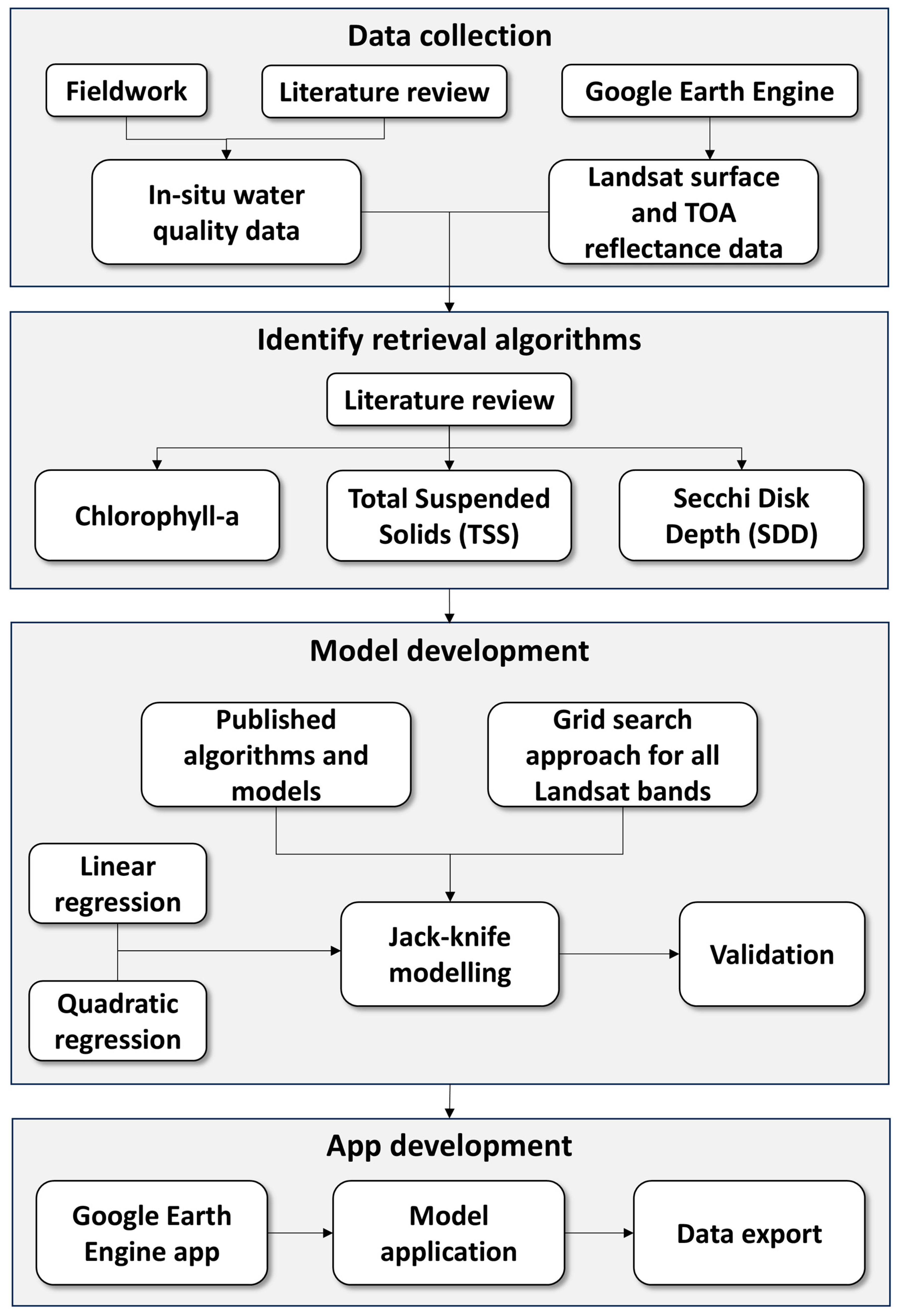
• Compile a ground truth database of water quality observations and Landsat satellite match-ups for East African lakes from existing studies supplemented by newly collected data.
• Identify existing Landsat water quality retrieval algorithms for chlorophyll-a, TSS, and SDD and assess their accuracy for East African lakes.
• Develop region-specific models where no suitable global models were available.
• Develop an easy-to-use Google Earth Engine application incorporating the best performing models for each parameter.

2. Methods

A summary of the overall methodology and modelling approach is provided in Figure 1.

2.1. Study Lakes

East African lakes range from freshwater to highly productive alkaline–saline soda lakes, largely due to the varied geology and climate of the East African Rift System and the endorheic nature of many lakes [2,37,38]. Lake morphology and water chemistry are influenced by volcanic and tectonic activity, as well as geothermal input from underground hot-spring systems [2,39]. The region is mostly characterised by bimodal rainfall, with a long (March to May) and a short (October to December) rainy season [40]; however, seasonality varies by latitude. Seasonality and interannual variability in climate are largely governed by the Indian Ocean Dipole, the intertropical convergence zone, and the El Niño–Southern Oscillation (ENSO) [40,41].

We selected seven study lakes across Ethiopia, Kenya, and bordering Kenya, Uganda, and Tanzania (Lake Victoria), covering a range of climatic, morphological, and water quality conditions (Figure 2A,

Table 1. Lake characteristics of the seven lakes used for model development. Lakes are ordered by latitude from north to south. Asl means above sea level. Data were obtained from the LAKEAtlas dataset [1].

Lake	Country	Freshwater or Saline	Average Surface Area (km2)	Average Depth (m)	Elevation (m asl)	Watershed Area (km2)
Ziway	Ethiopia	Freshwater	411.96	13.9	1636	7296.3
Chamo	Ethiopia	Freshwater	312.04	26.9	1109	1940.6
Turkana	Ethiopia/Kenya	Saline	7473.43	31.8	361	149,329.0
Baringo	Kenya	Freshwater	125.43	14.5	968	6604.4
Bogoria	Kenya	Saline	36.25	23.2	990	760.7
Oloidien	Kenya	Saline	5.21	8.9	1883	144.7
Victoria	Kenya/Uganda/ Tanzania	Freshwater	67,166.2	41.1	1134	265,373.0

). Lake selection was also determined by the availability of in situ water quality data for model development and is discussed further in Section 2.2. Four of the seven study lakes are freshwater, covering a range of productivities and turbidities. The freshwater lakes are Ziway and Chamo in Ethiopia, Baringo in Kenya, and Victoria spanning the borders of Kenya, Uganda, and Tanzania. The remaining three lakes are the alkaline–saline soda lakes Bogoria and Oloidien in Kenya, and Turkana spanning the border of Kenya and Ethiopia. Bogoria and Oloidien are important Lesser Flamingo feeding lakes and Turkana is the world’s largest alkaline–saline lake [42]. Lake characteristics are summarized in Table 1.

2.2. In Situ Data

In this study, we collated in situ water quality data for East African lakes from previous studies conducted by the authors or published in the literature (Figure 2A,

Table 2. Summary of the sampling dates and water quality parameters measured for each study lake prior to match-ups with Landsat reflectance data and data cleaning for model development. For lakes with source “This study”, data were either collected specifically for this study (Victoria and Baringo) or provided by co-authors and are not publicly available. See the “Data availability” statement for more information.

Lake	Date	Parameters	Number of In Situ Samples	Source
Ziway	24 January 2005– 4 January 2006	Chl-a	12	[42]
Chamo	25 March 2006– 8 February 2007	Chl-a	12	[42]
Turkana	1 September 2016– 4 September 2016	Chl-a, TSS, SDD	12	This study
Baringo	18 September 2023, 19 September 2023	Chl-a, TSS, SDD	15	This study
Bogoria	21 April 2010– 26 April 2010, 1 April 2012– 11 April 2012	Chl-a, TSS, SDD	39	[11,43]
Oloidien	31 March 2011– 1 April 2011	Chl-a, TSS, SDD	10	[43]
Victoria	13 September 2023	Chl-a, TSS, SDD	15	This study

). The literature search was conducted using Google Scholar, as well as global lake databases such as the Global Environmental Management System GEMStat [30] and the GLObal Reflectance community dataset for Imaging and optical sensing of Aquatic environments (GLORIA) [31]. Only studies providing georeferenced water quality data collected from the surface were included. Studies with sampling points along lake shorelines, or data without Landsat satellite match-ups, were excluded. Data from previous studies were obtained for two Ethiopian freshwater lakes, Chamo and Ziway, sampled monthly from 2005 to 2006 [43], and for three Kenyan saline lakes, Bogoria, Oloidien, and Turkana, sampled from 2010 to 2016 [11,44]. To ensure that a diverse range of water quality conditions were captured for East African lakes, a further two lakes were sampled for this study. Winam Gulf (also known as Nyanza Gulf), Lake Victoria, and Lake Baringo in Kenya were selected as optically complex freshwater lakes covering a range of chlorophyll-a and TSS concentrations. The addition of data from these lakes compliments the less turbid Ethiopian freshwater lakes and the Kenyan highly productive saline lakes (Figure 2).

In situ water samples were collected for Lake Victoria and Lake Baringo in September 2023 as close as possible to Landsat 8 and 9 overpass dates (14 September for Victoria and 15 September for Baringo). Sampling was conducted using a small boat, and two transects were performed for each lake. Transect locations were determined using the most recent cloud-free Sentinel-2 imagery to select sites that (a) enabled us to capture a gradient of TSS, chlorophyll-a, and SDD, and (b) were at least 1 km from the nearest shoreline to reduce the adjacency effects [45]. Water samples were collected between 9 a.m. and 2 p.m. local time under cloud-free conditions.

Data for Lake Victoria were collected from the Kenyan Winam Gulf region on 13 September 2023 (Figure 2C). Transect one started in the productive Kisumu Bay and headed 5 km out towards clearer waters (Figure 2D), sampling every 500 m to capture the gradient of chlorophyll-a concentrations at 10 sites. Transect two started in the sediment plume from a tributary (lat: −0.177, lon: 34.776) (Figure 2D) and headed out 2.5 km towards clear water, sampling every 500 m for 5 sites. Lake Baringo data were collected on 18 September 2023 and 19 September 2023. Transect one started in the turbid waters from the Endao and Molo tributaries in the south of the lake (Figure 2B) and continued for 5 km towards the clearer waters in the centre of the lake, with data collected every 500 m for 10 sites. Transect two covered 7 sites over 3.5 km from north to south across the north of the lake to sample the chlorophyll-a and TSS concentrations in the clearer waters.

Three replicate surface water samples were collected at each site for chlorophyll-a and TSS determination. Chlorophyll-a samples were stored in the dark below 4 °C to prevent chlorophyll degradation prior to analyses. Secchi disk depth was measured after water sample collection to limit the disturbance of the water. GPS coordinates were recorded for each site to enable match-ups with satellite imagery.

For chlorophyll-a determination, water samples were filtered through 47 mm 0.7 µm pore size glass fibre filter discs, and the filter discs were frozen overnight to aid the bursting of cells. Chlorophyll-a concentrations were then determined using the standard methods for the examination of water and wastewater trichromatic method [46] with a single beam Shimadzu UV-1800 spectrophotometer (Equation (1)):

$$Chlorophyll\text{-}a \mathrm{mg}/{\mathrm{m}}^3={\displaystyle \frac{\left(11.85\left(abs 664\right)-1.54\left(abs 647\right)-0.08\left(abs 630\right)\right)\times {EV}_L}{{SV}_{m^3}}}$$

(1)

where abs is absorbance, EV_L is extract volume in litres, and SV_m³ is the volume of the sample in m³. TSS concentrations were determined by filtering water samples through preweighed 47 mm 1.5 µm pore size 934-AH RTU Whatman glass fibre filter discs and drying in an oven at 105 °C, following the standard methods for the examination of water and wastewater total suspended solids protocol [46]. Sampling methods were the same for each lake, with the exception of TSS samples from saline lakes, which included an additional step of washing the filtered samples with distilled water to remove the salt content.

2.3. Satellite Imagery

Landsat Thematic Mapper (TM), Enhanced Thematic Mapper (ETM+) and Operational Land Imager (OLI) top-of-atmosphere (TOA) and surface reflectance (SR) images were accessed using the Google Earth Engine Python API [47]. Both TOA and SR data were acquired to identify the most suitable Landsat reflectance dataset available in Google Earth Engine for each water quality parameter. The images were Collection 2, Tier 1; datasets include only the highest quality images georeferenced within 12 m root mean square error (RMSE) and intercalibrated for consistency across Landsat sensors [48]. The surface reflectance images were atmospherically corrected using the LEDAPS algorithm for Landsat 5 (TM) and 7 (ETM+), and the LaSRC algorithm for Landsat 8 and 9 (OLI). The closest cloud-free satellite image match-ups were obtained for each study lake and sampling date. Ideally, match-ups between in situ data and satellite imagery would occur on the same date; however, to ensure the training dataset was of a sufficient size whilst limiting variations in water quality, match-ups within a 10-day window were selected [11]. Remaining clouds were masked using the pixel quality flags generated by the CFMASK algorithm [49]. In situ sampling sites covered by cloud, falling within the scan line error no data regions of Landsat 7 images or without Landsat image match-ups within a 10-day window, were removed from further analyses. Reflectance values were extracted from the corresponding pixels at the remaining 58 sampling locations for all visible and infrared satellite bands, from both TOA and SR imagery. Match-up differences between in situ sampling and Landsat imagery were as follows: Victoria, 1 day; Baringo, 4 days; Turkana, 6 days; Oloidien, 1 day; Bogoria, ranged from 2 to 7 days; Chamo, 3 to 4 days; and Ziway, ranging from same-day satellite overpass to 9 days.

2.4. Water Quality Retrieval Algorithms

A search of the literature was conducted to identify existing Landsat water quality retrieval algorithms for each parameter, which were then assessed for their suitability for East African lakes. The literature search was used to compile a list of both:

• Band algorithms (also known as spectral indices): mathematical equations comprising combinations of Landsat reflectance bands.
• Fully parameterised models: band algorithms that have been calibrated against ground-based observations to estimate model coefficients.

We chose to focus on models developed using band algorithms because these are simple to interpret and can be more easily implemented in an automated water quality monitoring tool than more complex models. The search of the literature was conducted using Google Scholar and the Google search engine. From the Landsat algorithms identified in the literature, we only selected those (i) developed for application to multiple waterbodies (global or regional); or (ii) specifically developed for East African waterbodies. Algorithms developed for individual lakes outside of East Africa were not evaluated. Eight algorithms were identified for chlorophyll-a, seven for TSS, and six for SDD (

Table 3. Band algorithms for estimating chlorophyll-a, TSS, and SDD from Landsat satellite imagery. The band combination colours relate to the respective reflectance band in Landsat imagery. The central wavelengths of each band are blue, 482 nm; green, 562 nm; red, 655 nm; NIR, 865 nm. Index names are provided; however, if no name is published, the band algorithm is named after the example reference. NDTI was tested for both TSS and SDD retrieval.

Parameter	Index	Band Combination	Example Reference
Chl-a	Normalised Difference Chlorophyll Index (NDCI)	${\displaystyle \frac{(NIR-Red)}{(NIR+Red)}}$	[25,27]
	2-Band Algorithm (2BDA)	${\displaystyle \frac{NIR}{Red}}$	[25]
	3-Band algorithm (3BDA)	$Blue-(Red\times Green)$	[50]
	Fluorescence Line Height Blue (FLH BLUE)	$\left(Green-Red\right)+(Blue-Red)$	[50]
	Surface Algal Bloom Index (SABI)	${\displaystyle \frac{(NIR-Red)}{(Blue+Green)}}$	[50,51]
	3BDA-like (KIVU)	$Blue-{\displaystyle \frac{Red}{Green}}$	[50]
	NRVI	${\displaystyle \frac{(\frac{Red}{NIR}-1)}{(\frac{Red}{NIR}+1)}}$	[52]
	Tebbs et al. (2013)	$\left(-135\right)+\left(451\right)\times \left({\displaystyle \frac{NIR}{Red}}\right)\pm 72$	[11]
TSS	Suspended Matter Index (SMI)	${\displaystyle \frac{(NIR+Red)}{2}}$	[53]
	Total Suspended Matter Index (TSMI)	${\displaystyle \frac{(Green+Red)}{2}}$	[54]
	Normalised Suspended Material Index (NSMI)	${\displaystyle \frac{(Red+Green-Blue)}{(Red+Green+Blue)}}$	[21]
	Normalised Difference Suspended Sediment Index (NDSSI)	${\displaystyle \frac{(Blue-NIR)}{(Blue+NIR)}}$	[21]
	2-Band Algorithm 1 (2BDA1)	${\displaystyle \frac{(Green-Blue)}{(Green+Blue)}}$	[17]
	2-Band Algorithm 2 (2BDA2)	${\displaystyle \frac{(Red-Blue)}{(Red+Blue)}}$	[17]
	Normalised Difference Turbidity Index (NDTI)	${\displaystyle \frac{(Red-Green)}{(Red+Green)}}$	[27]
SDD	Kloiber	${\displaystyle \frac{Blue}{(Red+Blue)}}$	[55]
	Lathrop	$Green$	[56]
	Normalised Difference Turbidity Index (NDTI)	${\displaystyle \frac{(Red-Green)}{(Red+Green)}}$	[27]
	Empirical Band Ratio (EBR)	${\displaystyle \frac{Blue}{Red}}$	[57]
	Lu2023T2	${\displaystyle \frac{Blue}{Red}}-{\displaystyle \frac{Blue}{Green}}$	[58]
	Song et al. (2022)	$-2.93\times \left({\displaystyle \frac{Red}{Blue}}\right)+2.83\times \left({\displaystyle \frac{Blue}{Green}}\right)+2.81$	[59]

).

Five of the eight chlorophyll-a algorithms, namely, NDCI, 2BDA, SABI, NRVI, and Tebbs et al. (2013), utilise the red-edge absorbance and reflectance peak characteristic of photosynthetic phytoplankton [17]. The 3BDA, FLU BLUE, and KIVU algorithms use only the visible reflectance more dominant in clearer waters with lower concentrations of phytoplankton. Similarly, the blue, green, and red bands are frequently used for TSS retrieval due to the strong visible reflectance of sediment-rich waters; however, NIR reflectance has also been shown to correlate with TSS at intermediate concentrations [21]. None of the SDD algorithms utilise the NIR band, likely due to the strongly absorbing features of water at these wavelengths when phytoplankton and surface sediments are not present.

The first published parameterised model directly tested in this study was the chlorophyll-a retrieval algorithm developed for Lake Bogoria, Kenya, by Tebbs et al. (2013) [11]. The model is a parameterised version of the 2BDA described in Table 3, utilising reflectance bands in the red and NIR. The Tebbs et al. (2013) method was the only Landsat retrieval model identified from our literature search that was developed specifically for an East African lake. The second published parameterised retrieval model compared with the band algorithms was the unified model for SDD retrieval developed by Song et al. (2022) [59] using data from 2235 lakes across the world. The model was trained using data from African lakes; however, the African continent has the lowest representation in the model. Published models were validated by applying them to the satellite image reflectance values and comparing the predicted water quality parameters with the observed values.

In addition to the algorithms identified from the literature, we assessed other suitable band algorithms using a grid-search approach to test the relationship between each water quality parameter and different single bands, band additions, band subtractions, band ratios, and normalised differences between bands.

2.5. Model Development and Validation

Pearson correlations were calculated between chlorophyll-a, TSS, and SDD to test for collinearity. Correlations above 0.7 were not identified, so models were developed for all parameters. For the chlorophyll-a models, values above 200 μg/L were removed as four datapoints from the saline lakes were significantly larger than most of the training data and had a strong influence on model performance. These samples have high uncertainty in chlorophyll-a values due to clumping of the cyanobacterial mats or dense subsurface layers, disturbance of these clumps during sampling, and the patchiness of the bloom conditions [11]. For the SDD models, only data collected in this study from Lake Victoria and Lake Baringo were used. Including data obtained from previous studies reduced the fit of all models, possibly due to differences in the sampling approaches, observer biases when reading the SDD, or due to the surface scums of cyanobacteria in the saline lakes that are disturbed during sampling [60], making match-ups with the satellite imagery less accurate. The summary statistics for the final in situ water quality data are provided in

Table 4. Summary statistics for the in situ water quality dataset used for model development and validation. Statistics are provided for individual lakes to show the range of conditions at each site, as well as the overall summary statistics for the modelling dataset.

Site	Parameter	Mean	Median	Min	Max	n
Baringo	Chl-a (μg/L)	9.44	9.44	5.43	12.8	15
	TSS (mg/L)	23.3	14.0	10.9	71.5	15
	SDD (m)	0.265	0.280	0.140	0.330	15
Bogoria	Chl-a (μg/L)	115.9	109.4	64.7	169.0	8
	TSS (mg/L)	44.8	46.5	23.0	68.0	8
	SDD (m)	-	-	-	-	-
Chamo	Chl-a (μg/L)	35.1	35.1	33.2	37.0	2
	TSS (mg/L)	-	-	-	-	-
	SDD (m)	-	-	-	-	-
Oloidien	Chl-a (μg/L)	129.8	129.8	129.8	129.8	1
	TSS (mg/L)	65.3	62.0	60.0	74.0	3
	SDD (m)	-	-	-	-	-
Turkana	Chl-a (μg/L)	4.13	3.09	1.66	9.69	5
	TSS (mg/L)	1.78	1.48	0.552	2.75	5
	SDD (m)	-	-	-	-	-
Victoria	Chl-a (μg/L)	25.5	20.0	9.72	69.8	15
	TSS (mg/L)	12.0	12.4	7.90	16.2	15
	SDD (m)	0.673	0.700	0.500	0.800	15
Ziway	Chl-a (μg/L)	38.2	36.3	34.0	47.2	5
	TSS (mg/L)	-	-	-	-	-
	SDD (m)	-	-	-	-	-
All sites	Chl-a (μg/L)	36.5	18.6	1.66	169.0	51
	TSS (mg/L)	24.1	13.9	0.552	74.0	46
	SDD (m)	0.469	0.415	0.140	0.800	30

.

A jack-knife modelling approach, also known as leave-one-out cross-validation, was used for model development and validation. This resampling approach removes one datapoint from analysis, trains the model on all other datapoints, and tests the accuracy of the model on the removed datapoint. Model training is repeated and validated using all datapoints, and an average value for all trained models is calculated. This method provides accurate estimates of variance and bias when developing models on small datasets [61,62]. Linear and quadratic polynomial regression models were developed for all parameters, using both raw and log-transformed response variables. Additionally, all models were developed and tested using both SR and TOA Landsat data to determine which Landsat reflectance dataset gave the best performance for each band ratio or model. Log-transformed chlorophyll-a values were better for all reflectance data models; however, for TSS and SDD, only the TOA reflectance data performed better with log-transformed response variables. The best performing models for each band algorithm, for example, linear regression with TOA reflectance, were validated by comparing the predicted values with the observed values. To assess the accuracy of each model, the root mean squared error (RMSE), mean absolute error (MAE), mean absolute percent error (MAPE), and bias were calculated. The performance metrics were calculated as follows:

$$RMSE=\sqrt{{\displaystyle \frac{{\sum }_{i=1}^n{\left(X_i-X_s\right)}^2}{n}}}$$

(2)

$$MAE={\displaystyle \frac{{\sum }_{i=1}^n\left|X_S-X_i\right|}{n}}$$

(3)

$$MAPE={\sum }_{i=i}^n{\displaystyle \frac{\left(X_i-X_S\right)}{X_i}}$$

(4)

$$Bias={\displaystyle \frac{1}{n}}{\sum }_{i=1}^n\left(X_S-X_i\right)$$

(5)

where X_i are the in situ observations, X_S are the satellite-derived parameters, and n is the number of match-ups between ground data and satellite data. The best performing models for each parameter were also verified using visual comparison of output maps with true colour satellite imagery.

2.6. App Development and Model Application

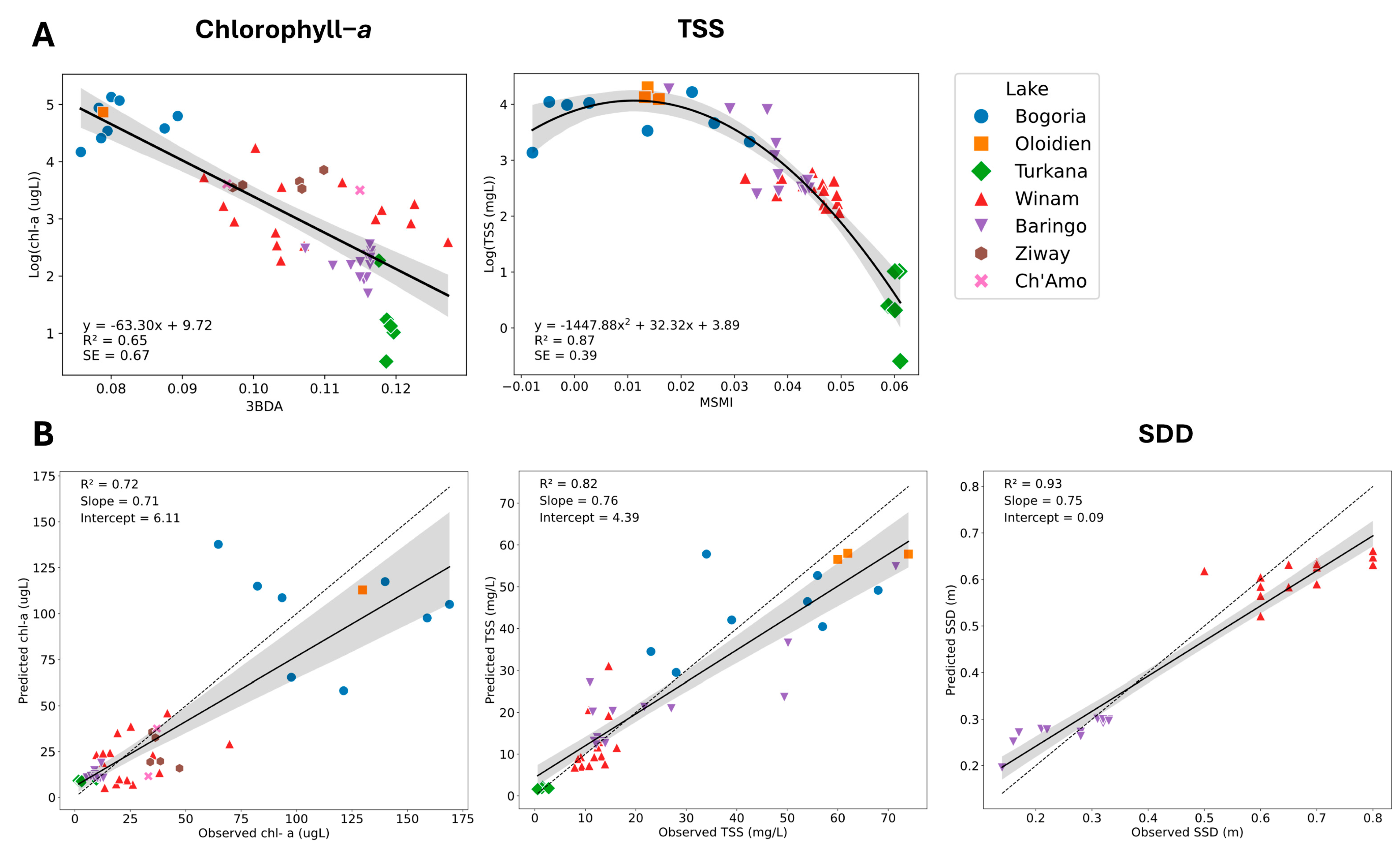
To ensure that the models developed in this study are accessible and can be used for water resource monitoring and management, a Google Earth Engine application was developed, named the LAndsat water QUality retrieval tool for East African lakes (LAQUA). The LAQUA application can be accessed at (https://emmatebbs.users.earthengine.app/view/laqua). We chose Google Earth Engine because it provides access to archives of Landsat imagery, facilitates faster analyses with cloud processing, and provides interactive tools for applying the models directly to a region of interest. Application development steps are summarised in Figure 3. Landsat 5, 7, 8, and 9 TOA Collection 2 Tier 1 images were filtered to remove imagery with more than 10% cloud cover for the study region, and the remaining clouds were masked using the CFMASK pixel quality flags described in the satellite imagery section. Water pixels were identified using the Modified Normalised Difference Water Index (MNDWI) [15]. The MNDWI is calculated as follows:

$$MNDWI={\displaystyle \frac{Green-SWIR}{Green+SWIR}}$$

(6)

where Green is reflectance measured between 520 nm and 600 nm, and SWIR (shortwave infrared) is reflectance measured between 1550 nm and 1750 nm by the Landsat satellites. Values greater than 0 indicate water; however, a threshold for 0.4 was used to more accurately distinguish water from other pixels [63], masking land, floating vegetation, and dense cyanobacterial surface scums.

The best performing water quality retrieval models were applied to the Landsat reflectance bands, and the median value for each pixel for each month was calculated to produce monthly maps for the selected date range. The monthly maps were averaged over the region of interest to produce lake-wide mean monthly time series of chlorophyll-a, TSS, and SDD. Monthly averages were plotted for each water quality parameter for the desired date range within the application user interface. Maps were produced within the map panel to visualise the median true colour image, chlorophyll-a concentration, TSS concentration, and SDD for the previous two months. The two-month medians were used for more effective visualisation of the larger lakes covered by multiple Landsat tiles to mitigate the influence of increased cloud cover and no data regions. Visualising retrieval maps for the largest lakes, such as Lake Victoria, proved more challenging, and cloud-free monthly composites covering the whole lake were less common. Despite this limitation for the largest lakes, lake-wide monthly averages were estimated using the regions covered by Landsat imagery for each month.

The user simply defines a study region using one of the polygon geometry tools and selects a start and end date using the calendar tools. Polygons can be drawn around whole lakes or individual regions of a waterbody, or a point can be used to extract data from a single pixel. Time series graphs can be saved as a scalable vector graphic (SVG) or a portable network graphic (PNG), and data can be exported as a comma-separated values (CSV) file for use in further analyses. The retrieval models can be applied to Landsat 5, 7, 8, and 9 imagery from January 2000 to the present day for use in temporal studies and for identifying changes over time.

3. Results

Table 5. Model validation results between observed and predicted values for the published band algorithms and models, as well as the best performing grid-search models for each parameter developed in this study. For each band algorithm or model, only the results for the best linear or quadratic regression model and the most suitable reflectance data, either surface reflectance (SR) or top-of-atmosphere (TOA), are provided. Bold text highlights the best overall model for each parameter.

Parameter	Algorithm	Model Type	Reflectance	Intercept	R2	p-Value	RMSE	MAE	MAPE	Bias
Chl-a (μg/L)	NDCI	Linear	SR	6.13	0.520	0.000	31.6	19.2	64.8	−4.44
	2BDA	Quadratic	SR	6.09	0.540	0.000	30.2	18.1	59.9	−5.84
	3BDA	Linear	TOA	6.11	0.717	0.000	22.9	14.7	59.9	−4.61
	FLH BLUE	Quadratic	SR	19.0	0.105	0.020	43.2	25.9	118.6	−15.42
	SABI	Quadratic	SR	9.43	0.589	0.000	28.5	18.3	62.7	−8.22
	KIVU	Quadratic	TOA	12.2	0.385	0.000	34.7	21.1	95.1	−10.50
	NRVI	Linear	TOA	8.10	0.470	0.000	32.4	19.8	67.5	−6.59
	Tebbs et al. (2013)	Linear	TOA	77.9	0.551	0.000	150.1	118.4	293.2	108.24
	This study—NDCI-SABI ratio	Linear	SR	6.49	0.578	0.000	28.9	17.3	56.8	−3.29
TSS (mg/L)	SMI	Quadratic	TOA	14.8	0.043	0.169	21.9	14.4	102.4	−7.67
	TSMI	Quadratic	TOA	11.7	0.253	0.000	18.8	12.1	84.8	−4.85
	NSMI	Quadratic	TOA	13.5	0.147	0.008	20.4	12.9	100.3	−6.49
	NDSSI	Linear	TOA	15.7	0.352	0.000	16.9	12.9	58.2	−0.36
	2BDA1	Quadratic	TOA	15.8	0.005	0.658	22.5	14.6	112.9	−7.55
	2BDA2	Quadratic	TOA	11.9	0.232	0.001	19.3	12.3	89.2	−6.03
	NDTI	Quadratic	TOA	9.8	0.187	0.003	21.2	12.9	78.3	−5.64
	This study—MSMI	Quadratic	TOA	4.39	0.822	0.000	9.00	5.91	28.3	−1.25
SDD (m)	Kloiber	Quadratic	TOA	0.025	0.913	0.000	0.065	0.050	12.6	−0.003
	Lathrop	Quadratic	SR	0.070	0.850	0.000	0.084	0.066	17.1	−0.000
	Song et al. (2022)	Linear	TOA	0.091	0.933	0.000	0.073	0.058	13.3	−0.025
	NDTI	Quadratic	TOA	0.043	0.889	0.000	0.073	0.051	12.8	−0.006
	EBR	Quadratic	TOA	0.024	0.904	0.000	0.068	0.054	13.8	−0.004
	Lu2023T2	Quadratic	TOA	0.035	0.875	0.000	0.077	0.056	12.6	−0.004
	This study—Red-Blue ratio	Quadratic	TOA	0.025	0.921	0.000	0.061	0.046	11.3	−0.003

provides a summary of the best performing models for each water quality parameter. Models for chlorophyll-a, TSS, and SDD are then discussed in further detail in the relevant Section 3.1, Section 3.2, Section 3.3, Section 3.4, which describe the validation of the best performing models for each water quality parameter using the Kenyan lakes Baringo and Bogoria as case studies, the comparison between the predicted values for each lake with those reported in the published literature, and the validation of the Google Earth Engine app using true colour imagery.

3.1. Chlorophyll-a

The best performing chlorophyll-a model was the three-band algorithm (3BDA) with a linear regression using top-of-atmosphere imagery (R² = 0.717, p < 0.001, RMSE = 22.917 μg/L) (Table 5, Figure 4). The model underestimates concentrations by an average of 4.6 ug/L, though it performs significantly better and has lower error than the next best performing band algorithm, the Surface Algal Bloom Index (SABI) (R² = 0.589, p < 0.001, RMSE = 28.528 μg/L). The Tebbs et al. (2013) model (R² = 0.551, p < 0.001, RMSE = 150.084 μg/L), a parameterised version of the 2BDA (R² = 0.540, p < 0.001, RMSE = 30.168 μg/L), had a higher R² than the 2BDA parameterised to the dataset in this study; however, it overestimated values by an average of 108.2 μg/L and had a significantly larger error. The positive bias could be attributed to the Tebbs et al. (2013) model training dataset containing data from a single highly productive saline lake with values ranging from 0 to more than 800 μg/L, considerably larger than the training data used in this study. The best performing 3BDA model is described in Equation (7):

$$log\left(Chlorophyll\text{-}a\right)=-63.2976\times \left(Blue-\left(Red\times Green\right)\right)+9.7195$$

(7)

where Blue is reflectance measured at 485 nm by Landsat 5 and 7 or 480 nm by Landsat 8 and 9, Red is reflectance measured at 660 nm by Landsat 5 and 7 or 655 nm by Landsat 8 and 9, and Green is reflectance measured at 560 nm by Landsat 5, 7, 8, and 9.

3.2. Total Suspended Solids

The best performing TSS model was developed in this study and is based on a modified version of the Suspended Matter Index (SMI), henceforth referred to as the Modified Suspended Matter Index (MSMI) (Table 5, Figure 4). MSMI subtracts the SMI values from an additional blue band, greatly improving the TSS prediction performance (R² = 0.822, p < 0.001, RMSE = 9.006 mg/L). The equation slightly underestimates TSS values by an average of 1.246 mg/L. All models performed best with log-transformed TSS data and top-of-atmosphere imagery. The TSS band algorithms identified from the literature performed poorly, with R² values ranging from 0.005 (2BDA1) to 0.352 (NDSSI). The best performing MSMI quadratic model is described in Equation (8):

$$log\left(TSS\right)=-\left(32.3214\times \left(Blue-SMI\right)\right)+\left(-1447.8775\times {\left(Blue-SMI\right)}^2\right)+3.8861$$

(8)

where SMI is calculated using Equation (9):

$$SMI={\displaystyle \frac{(NIR+Red)}{2}}$$

(9)

3.3. Secchi Disk Depth

The best performing SDD retrieval model was the linear model developed by Song et al. (2022) using top-of-atmosphere imagery (R² = 0.933, p < 0.001, RMSE = 0.073 m) (Table 5, Figure 4). All other SDD models performed well, with R² values ranging from 0.850 (Lathrop) to 0.921 (red–blue ratio developed in this study) and small negative biases in predicted values. With the exception of the Song et al. (2022) model, a quadratic model best described the relationship between the band algorithms and log-transformed Secchi depth. Only the Lathrop model performed better with Landsat surface reflectance data. Despite all models performing well, the Song et al. (2022) model was developed using data from 2235 global lakes and, thus, is likely to be more robust when applied to lakes outside of the training dataset used in this study. The Song et al. (2022) model equation is described in Table 3.

3.4. Google Earth Engine App and Validation

The best performing models for each water quality parameter were further validated through visual comparison with true colour satellite imagery using the Google Earth Engine app. Models were applied to Landsat imagery from September 2023 for the turbid freshwater Lake Baringo and the highly productive alkaline–saline Lake Bogoria (Figure 5). Chlorophyll-a concentrations showed distinct differences between the lakes, with Baringo averaging concentrations of less than 20 μg/L and Bogoria exceeding concentrations of 100 μg/L. Total suspended solids were highest in the southwest region of Lake Baringo, where the main tributaries enter the lake. Similarly, TSS values were highest for Bogoria in the north of the lake near the Waseges–Sandai river delta [64], as well as near the dense cyanobacterial blooms in the south of the lake. Secchi disk depths decreased in areas with high suspended solids. The spatial patterns and concentrations of each parameter agree with those observed in previous studies for both lakes [11,65]. Further visual validation was conducted for lakes across Ethiopia, Kenya, Uganda, Tanzania, and Malawi using the Google Earth Engine application. The retrieval models accurately detected algal blooms and high-concentration sediment plumes visible in true colour imagery.

4. Discussion

This study identified 21 published Landsat band algorithms for water quality retrieval and evaluated their performance for East African lakes. Model accuracy was assessed using a dataset of 58 observations from 7 lakes, collated from existing studies supplemented by new data collection. Existing published algorithms were compared with newly developed models identified using a grid-search approach. The most suitable band algorithms were the following:

• For chlorophyll-a: a parameterised version of the three-band algorithm (3BDA).
• For total suspended solids (TSS): a modified version of the Suspended Matter Index (SMI) developed in this study with an additional blue band.
• For Secchi disk depth (SDD): an existing global model developed by Song et al. (2022).

The best performing models were incorporated into a Google Earth Engine application for easy and accessible use for researchers, water resource managers, and policymakers. The application works globally for all inland lakes and waterbodies; however, the chlorophyll-a and TSS models have been parameterised for more accurate water quality retrieval in East African lakes. The SDD model described by Song et al. (2022) was developed using data from 2235 lakes worldwide and is suitable for all lakes globally.

The 3BDA chlorophyll-a algorithm utilises the blue, red, and green Landsat satellite bands. Interestingly, the algorithm does not utilise reflectance in the near-infrared (NIR) band despite strong correlations being identified between NIR reflectance and chlorophyll-a concentrations in other studies [11,14]. Landsat satellites were designed for monitoring terrestrial surfaces; the NIR band measures reflectance at higher wavelengths beyond the red edge than sensors specifically developed for water quality monitoring [17]. NIR reflectance due to phytoplankton at these higher wavelengths is offset by the highly absorbing properties of water. Thus, with Landsat satellites, NIR reflectance is likely a better predictor of chlorophyll-a in highly productive hypertrophic waters with a stronger NIR backscattering peak [11] than for waters with a maximum chlorophyll concentration of 200 ug/L used for model development in this study. The 3BDA algorithm instead utilises the backscattering in the green and absorbance in the red wavelengths associated with chlorophyll-a [66]. The linear model can extrapolate beyond the training data range and is suitable for a range of lake types, including both clear and turbid freshwater lakes, and it can detect high chlorophyll-a concentrations in productive saline lakes. However, the Tebbs et al. (2013) model may be more suitable for highly productive saline lakes given the higher chlorophyll-a concentrations included in the training data.

The MSMI TSS retrieval algorithm developed in this study utilises the blue, red, and NIR Landsat bands. The inclusion of the blue band greatly improved the performance of the Suspended Matter Index (SMI). Of the best performing water quality retrieval models for each parameter, MSMI was the only model that was developed using a quadratic regression model. Therefore, the model is accurate for the training data range between 0 and 70 mg/L TSS; however, due to the curved nature of the quadratic regression, the model likely underestimates TSS values higher than 70 mg/L (Figure 4). The poor performance observed for the published TSS band algorithms could be attributed to the previous studies developing models for other regions [53,54] and the optically complex nature of TSS retrieval [67]. The published band algorithms are not robust when applied to other lakes where the constituent organic and inorganic suspended solids may differ. Thus, regional models suitable for the lakes of interest, such as the MSMI, or global models trained on a range of optical water types, are required.

The SDD models had the best overall model performance. High model accuracy could be attributed to the inclusion of just Lake Victoria and Lake Baringo data in model development and validation. The other lakes were excluded due to significantly lower performance of all models, possibly due to differences in observer bias and the effects of disturbing cyanobacterial surface scums when sampling productive saline lakes [60]. Additionally, SDD shows low variation under stable hydrological conditions with minimal human activity and is less likely to be influenced by differences in match-up windows between in situ sampling and satellite imagery [23]. The global model described by Song et al. (2022) was the best performing Secchi disk depth retrieval model. Therefore, despite including fewer lakes in the model validation, there can be high confidence in the robustness of the SDD retrieval model and its suitability for East African lakes.

The three best performing models utilised top-of-atmosphere imagery. This suggests that the LEDAPS and LaSRC atmospheric correction methods applied to Landsat imagery are not suitable for inland waterbodies in East Africa, likely because they were designed to resolve atmospheric effects over land [68]. Atmospheric correction is extremely challenging over inland waters, and even the best performing atmospheric correction models have large uncertainties in reflectances (20–30%) that translate to large uncertainties in chl-a and TSS (25–70%) [69]. Other atmospheric corrections may be more suitable than the LEDAPS and LaSRC methods; however, exploring the suitability of atmospheric correction methods was outside the scope of this study. The literature review performed to collate suitable in situ data also confirmed the lack of water quality data for East African lakes [30,31], particularly surface water measurements suitable for satellite match-ups. The lack of surface water measurements explains why very few “global” algorithms incorporate data from African lakes. Without representative data for the optical water types present in East African waterbodies and the atmospheric effects present in the region, global algorithms should be applied to East African lakes with caution. Furthermore, the methods developed in this study may not be as accurate for lake types not included in the training data. The seven lakes used for modelling included both clear and turbid freshwater lakes, as well as productive alkaline–saline soda lakes, covering a range of optical water types. However, the deepest, clearest lakes such as Lake Tanganyika, shallow, seasonal pans, and lakes outside of the training data region require further model validation with in situ water quality data. Future work should prioritise the collection of water quality data for a wider range of African waterbodies and explore machine learning methods for both the development of water quality retrieval methods and for selecting the optimal band ratios for different optical water types in East African lakes [26,52].

The three water quality retrieval models described here showed strong predictive performance, chlorophyll-a (R² = 0.717, p < 0.001, RMSE = 22.917 μg/L), TSS (R² = 0.822, p < 0.001, RMSE = 9.006 mg/L), and Secchi disk depth (R² = 0.933, p < 0.001, RMSE = 0.073 m); however, the quantification of relationships between parameters and reflectance was limited by several factors. Match-up windows between satellite imagery and in situ data varied for each study lake. The closest match-up was on the same day as in situ sampling and the most distant match-up was 9 days. The longer the time period between the in situ data collection and the nearest cloud-free satellite image, the greater the likelihood that the water quality will have changed at the sampling point. This will lead to an underestimation of the R² value and an overestimation of the RMSE and MAE values. Additionally, in situ point sampling data were matched with the 30 by 30 m Landsat pixels in which they fell. The in situ data provide a good indication of the water quality conditions within the Landsat pixel; however, the reflectance measured by the Landsat satellites is averaged over the pixel area [8]. Variations in water quality within the pixel area and the location of the in situ sampling point within the pixel add further uncertainties to model development. Despite these limitations, good model performance was achieved for the three water quality parameters.

5. Conclusions

In this study, 21 published Landsat band algorithms for water quality retrieval were evaluated for East African lakes using a dataset of 58 in situ observations from 7 lakes. Existing published algorithms were compared with newly developed models to identify the most suitable Landsat water quality retrieval models for East African lakes: for chlorophyll-a retrieval, the three-band algorithm, parameterised using data for East African lakes, proved the most suitable (R² = 0.717, p < 0.001, RMSE = 22.917 μg/L); for TSS retrieval, a novel index developed in this study, the Modified Suspended Matter Index (MSMI) was the most accurate (R² = 0.822, p < 0.001, RMSE = 9.006 mg/L); and for SDD estimation, an existing global model was the most accurate (R² = 0.933, p < 0.001, RMSE = 0.073 m). Additionally, we developed an easy-to-use Google Earth Engine application (LAQUA) for applying the retrieval models to a time series of Landsat images to obtain monthly averages for a chosen waterbody, improving the accessibility of water quality remote sensing for water quality practitioners in East Africa for the first time. The LAQUA application provides a valuable resource that water managers can use, without any prior remote sensing experience, to fill data gaps for lakes that lack regular monitoring, quantify multiple water quality parameters simultaneously, investigate long-term trends and seasonality using the multidecadal archive of Landsat satellite imagery, conduct multilake comparisons, explore spatial gradients within lakes, and provide quantitative evidence to support water resource management decision making. When combined with other in situ or satellite observations, the outputs of LAQUA can be applied to a wide range of applications including assessing the influence of nutrient inputs on harmful algal bloom occurrence and monitoring climate and land-use change impacts on lake ecosystems. Both the app and the source code are freely available to the research community, and we envisage this as a continually evolving resource for those working on remote sensing of African lakes. For example, in future work, we plan to include additional water quality parameters, such as surface temperature and turbidity, and additional datasets from other satellite sensors, such as Sentinel-2, to continue to improve the accessibility of remote sensing for water quality monitoring.

References

1. Lehner, B.; Messager, M.L.; Korver, M.C.; Linke, S. Global Hydro-Environmental Lake Characteristics at High Spatial Resolution. Sci. Data 2022, 9, 351. [Google Scholar] [CrossRef]
2. Fazi, S.; Butturini, A.; Tassi, F.; Amalfitano, S.; Venturi, S.; Vazquez, E.; Clokie, M.; Wanjala, S.W.; Pacini, N.; Harper, D.M. Biogeochemistry and Biodiversity in a Network of Saline–Alkaline Lakes: Implications of Ecohydrological Connectivity in the Kenyan Rift Valley. Ecohydrol. Hydrobiol. 2018, 18, 96–106. [Google Scholar] [CrossRef]
3. Swenson, S.; Wahr, J. Monitoring the Water Balance of Lake Victoria, East Africa, from Space. J. Hydrol. 2009, 370, 163–176. [Google Scholar] [CrossRef]
4. Musie, M.; Momblanch, A.; Sen, S. Exploring Future Global Change-Induced Water Imbalances in the Central Rift Valley Basin, Ethiopia. Clim. Chang. 2021, 164, 47. [Google Scholar] [CrossRef]
5. Walker, D.; Shutler, J.D.; Morrison, E.H.J.; Harper, D.M.; Hoedjes, J.C.B.; Laing, C.G. Quantifying Water Storage within the North of Lake Naivasha Using Sonar Remote Sensing and Landsat Satellite Data. Ecohydrol. Hydrobiol. 2022, 22, 12–20. [Google Scholar] [CrossRef]
6. Morara, G.; Omondi, R.; Obegi, B.; Getabu, A.; Njiru, J.; Rindoria, N. Water Level Fluctuations and Fish Yield Variations in Lake Naivasha, Kenya: The Trends and Relationship. J. Fish. Environ. 2022, 46, 13–27. [Google Scholar]
7. Plisnier, P.D.; Kayanda, R.; MacIntyre, S.; Obiero, K.; Okello, W.; Vodacek, A.; Cocquyt, C.; Abegaz, H.; Achieng, A.; Akonkwa, B.; et al. Need for Harmonized Long-Term Multi-Lake Monitoring of African Great Lakes. J. Great Lakes Res. 2023, 49, 101988. [Google Scholar] [CrossRef]
8. Wegman, M.; Leutner, B.; Dech, S. Remote Sensing and GIS for Ecologists; Pelagic Publishing Ltd.: London, UK, 2016. [Google Scholar]
9. Tebbs, E.; Byrne, A.; Lomeo, D.; Thompson, H.; Owoko, W.; Nyaga, J.; Ongore, C.; Last, J.; Migeni, Z.; Everitt, L. Satellite Earth Observation for the Sustainable Management of the African Great Lakes; King’s College: London, UK, 2023. [Google Scholar]
10. Ermida, S.L.; Mantas, V.; Göttsche, F. Google Earth Engine Open-Source Code for Land Surface Temperature Estimation from the Landsat Series. Remote Sens. 2020, 12, 1471. [Google Scholar] [CrossRef]
11. Tebbs, E.J.; Remedios, J.J.; Harper, D.M. Remote Sensing of Chlorophyll-a as a Measure of Cyanobacterial Biomass in Lake Bogoria, a Hypertrophic, Saline—Alkaline, Flamingo Lake, Using Landsat ETM+. Remote Sens. Environ. 2013, 135, 92–106. [Google Scholar] [CrossRef]
12. Wang, C.; Chen, S.; Li, D.; Wang, D.; Liu, W.; Yang, J. A Landsat-Based Model for Retrieving Total Suspended Solids Concentration of Estuaries and Coasts in China. Geosci. Model Dev. 2017, 10, 4347–4365. [Google Scholar] [CrossRef]
13. Harrington, J.A.; Schiebe, F.R.; Nix, J.E. Remote Sensing of Lake Chicot, Arkansas: Monitoring Suspended Sediments, Turbidity, and Secchi Depth with Landsat MSS Data. Remote Sens. Environ. 1992, 39, 15–27. [Google Scholar] [CrossRef]
14. Mishra, S.; Mishra, D.R. Normalized Difference Chlorophyll Index: A Novel Model for Remote Estimation of Chlorophyll-a Concentration in Turbid Productive Waters. Remote Sens. Environ. 2012, 117, 394–406. [Google Scholar] [CrossRef]
15. Xu, H. Modification of Normalised Difference Water Index (NDWI) to Enhance Open Water Features in Remotely Sensed Imagery. Int. J. Remote Sens. 2006, 27, 3025–3033. [Google Scholar] [CrossRef]
16. Tavora, J.; Jiang, B.; Kiffney, T.; Bourdin, G.; Gray, P.C.; de Carvalho, L.S.; Hesketh, G.; Schild, K.M.; de Souza, L.F.; Brady, D.C.; et al. Recipes for the Derivation of Water Quality Parameters Using the High-Spatial-Resolution Data from Sensors on Board Sentinel-2A, Sentinel-2B, Landsat-5, Landsat-7, Landsat-8, and Landsat-9 Satellites. J. Remote Sens. 2023, 3, 0049. [Google Scholar] [CrossRef]
17. Xiao, Y.; Chen, J.; Xu, Y.; Guo, S.; Nie, X.; Guo, Y.; Li, X.; Hao, F.; Fu, Y.H. Monitoring of Chlorophyll-a and Suspended Sediment Concentrations in Optically Complex Inland Rivers Using Multisource Remote Sensing Measurements. Ecol. Indic. 2023, 155, 111041. [Google Scholar] [CrossRef]
18. Kiage, L.M.; Douglas, P. Linkages between Land Cover Change, Lake Shrinkage, and Sublacustrine Influence Determined from Remote Sensing of Select Rift Valley Lakes in Kenya. Sci. Total Environ. 2020, 709, 136022. [Google Scholar] [CrossRef] [PubMed]
19. Balasubramanian, S.V.; Pahlevan, N.; Smith, B.; Binding, C.; Schalles, J.; Loisel, H.; Gurlin, D.; Greb, S.; Alikas, K.; Randla, M.; et al. Robust Algorithm for Estimating Total Suspended Solids (TSS) in Inland and Nearshore Coastal Waters. Remote Sens. Environ. 2020, 246, 111768. [Google Scholar] [CrossRef]
20. Turner, A.; Millward, G.E. Suspended Particles: Their Role in Estuarine Biogeochemical Cycles. Estuar. Coast. Shelf Sci. 2002, 55, 857–883. [Google Scholar] [CrossRef]
21. Adjovu, G.E.; Stephen, H.; James, D.; Ahmad, S. Measurement of Total Dissolved Solids and Total Suspended Solids in Water Systems: A Review of the Issues, Conventional, and Remote Sensing Techniques. Remote Sens. 2023, 15, 3534. [Google Scholar] [CrossRef]
22. Song, K.; Li, L.; Wang, Z.; Liu, D.; Zhang, B.; Xu, J.; Du, J.; Li, L.; Li, S.; Wang, Y. Retrieval of Total Suspended Matter (TSM) and Chlorophyll-a (Chl-a) Concentration from Remote-Sensing Data for Drinking Water Resources. Environ. Monit. Assess. 2012, 184, 1449–1470. [Google Scholar] [CrossRef]
23. Zhang, Y.; Zhang, Y.; Shi, K.; Zhou, Y.; Li, N. Remote Sensing Estimation of Water Clarity for Various Lakes in China. Water Res. 2021, 192, 116844. [Google Scholar] [CrossRef] [PubMed]
24. Alba, A.C.G.; Anabella, B.C.F.; Marcelo, C.S.; Andrea, D.G.A.; Ivana, E.T.; Iba, E.; Sandra, E.T.; Michal, F.S.; Pascal, U.B.; Paz, L.; et al. Spectral Monitoring of Algal Blooms in an Eutrophic Lake Using Sentinel-2A. In Proceedings of the IGARSS 2019—2019 IEEE International Geoscience and Remote Sensing Symposium, Yokohama, Japan, 28 July–2 August 2019; pp. 306–309. [Google Scholar]
25. Buma, W.G.; Lee, S. Il Evaluation of Sentinel-2 and Landsat 8 Images for Estimating Chlorophyll-a Concentrations in Lake Chad, Africa. Remote Sens. 2020, 12, 2437. [Google Scholar] [CrossRef]
26. Smith, B.; Pahlevan, N.; Schalles, J.; Ruberg, S.; Errera, R.; Ma, R.; Giardino, C.; Bresciani, M.; Barbosa, C.; Moore, T.; et al. A Chlorophyll-a Algorithm for Landsat-8 Based on Mixture Density Networks. Front. Remote Sens. 2021, 1, 623678. [Google Scholar] [CrossRef]
27. Singh, R.; Saritha, V.; Pande, C.B. Monitoring of Wetland Turbidity Using Multi-Temporal Landsat-8 and Landsat-9 Satellite Imagery in the Bisalpur Wetland, Rajasthan, India. Environ. Res. 2024, 241, 117638. [Google Scholar] [CrossRef] [PubMed]
28. Byrne, A.; Tebbs, E.J.; Njoroge, P.; Nkwabi, A.; Chadwick, M.A.; Freeman, R.; Harper, D.; Norris, K. Productivity Declines Threaten East African Soda Lakes and the Iconic Lesser Flamingo. Curr. Biol. 2024, 34, 1786–1793.e4. [Google Scholar] [CrossRef] [PubMed]
29. Ballatore, T.J.; Bradt, S.R.; Olaka, L.; Cózar, A.; Loiselle, S.A. Remote Sensing of African Lakes: A Review. In Remote Sensing of the African Seas; Springer: Dordrecht, The Netherlands, 2014; pp. 403–422. [Google Scholar]
30. UNEP. The Global Water Quality Database; GEMStat: Koblenz, Germany, 2020. [Google Scholar]
31. Lehmann, M.K.; Gurlin, D.; Pahlevan, N.; Alikas, K.; Anstee, J.; Balasubramanian, S.V.; Barbosa, C.C.F.; Binding, C.; Bracher, A.; Bresciani, M.; et al. GLORIA—A Globally Representative Hyperspectral in Situ Dataset for Optical Sensing of Water Quality. Sci. Data 2023, 10, 100. [Google Scholar] [CrossRef] [PubMed]
32. Arias-Rodriguez, L.F.; Tüzün, U.F.; Duan, Z.; Huang, J.; Tuo, Y.; Disse, M. Global Water Quality of Inland Waters with Harmonized Landsat-8 and Sentinel-2 Using Cloud-Computed Machine Learning. Remote Sens. 2023, 15, 1390. [Google Scholar] [CrossRef]
33. Kaufman, Y.J. Atmospheric Effects on Remote Sensing of Surface Reflectance. Remote Sens. Crit. Rev. Technol. 1984, 475, 20–33. [Google Scholar] [CrossRef]
34. Majozi, N.P.; Salama, M.S.; Bernard, S.; Harper, D.M.; Habte, M.G. Remote Sensing of Euphotic Depth in Shallow Tropical Inland Waters of Lake Naivasha Using MERIS Data. Remote Sens. Environ. 2014, 148, 178–189. [Google Scholar] [CrossRef]
35. Kneubühler, M.; Frank, T.; Kellenberger, T.; Pasche, N.; Schmid, M. Mapping Chlorophyll-a in Lake Kivu with Remote Sensing Methods. In Proceedings of the Envisat Symposium 2007, Montreux, Switzerland, 23–27 April 2007. [Google Scholar] [CrossRef]
36. Ndungu, J.; Monger, B.C.; Augustijn, D.C.M.; Hulscher, S.J.M.H.; Kitaka, N.; Mathooko, J.M. Evaluation of Spatio-Temporal Variations in Chlorophyll-a in Lake Naivasha, Kenya: Remote-Sensing Approach. Int. J. Remote Sens. 2013, 34, 8142–8155. [Google Scholar] [CrossRef]
37. Nicholson, S.E. Climate and Climatic Variability of Rainfall over Eastern Africa. Rev. Geophys. 2017, 55, 590–635. [Google Scholar] [CrossRef]
38. Ogega, O.M.; Mbugua, J.; Misiani, H.O.; Nyadawa, M.; Scoccimarro, E.; Endris, H.S. Detection and Attribution of Lake Victoria’s Water-Level Fluctuations in a Changing Climate. Preprints 2021, 2021070575. [Google Scholar] [CrossRef]
39. Tarits, C.; Renaut, R.W.; Tiercelin, J.J.; Le Hérissé, A.; Cotten, J.; Cabon, J.Y. Geochemical Evidence of Hydrothermal Recharge in Lake Baringo, Central Kenya Rift Valley. Hydrol. Process. 2006, 20, 2027–2055. [Google Scholar] [CrossRef]
40. Seka, A.M.; Zhang, J.; Ayele, G.T.; Demeke, Y.G.; Han, J.; Prodhan, F.A. Spatio-Temporal Analysis of Water Storage Variation and Temporal Correlations in the East Africa Lake Basins. J. Hydrol. Reg. Stud. 2022, 41, 101094. [Google Scholar] [CrossRef]
41. WWF. Climate Change Impacts on East Africa. 2006. Available online: https://www.wwf.or.jp/activities/lib/pdf_climate/environment/east_africa_climate_change_impacts_final.pdf (accessed on 2 February 2024).
42. Schagerl, M. Soda Lakes of East Africa; Springer: Cham, Switzerland, 2016; ISBN 9783319286204. [Google Scholar]
43. Tilahun, G.; Ahlgren, G. Seasonal Variations in Phytoplankton Biomass and Primary Production in the Ethiopian Rift Valley Lakes Ziway, Awassa and Chamo—The Basis for Fish Production. Limnologica 2010, 40, 330–342. [Google Scholar] [CrossRef]
44. Tebbs, E.J.; Remedios, J.J.; Avery, S.T.; Rowland, C.S.; Harper, D.M. Regional Assessment of Lake Ecological States Using Landsat: A Classification Scheme for Alkaline-Saline, Flamingo Lakes in the East African Rift Valley. Int. J. Appl. Earth Obs. Geoinf. 2015, 40, 100–108. [Google Scholar] [CrossRef]
45. Kahru, M.; Kudela, R.M.; Anderson, C.R.; Manzano-Sarabia, M.; Mitchell, B.G. Evaluation of Satellite Retrievals of Ocean Chlorophyll-a in the California Current. Remote Sens. 2014, 6, 8524–8540. [Google Scholar] [CrossRef]
46. Baird, R.; Bridgewater, L. Standard Methods for the Examination of Water and Wastewater, 23rd ed.; American Public Health Association: Washington, DC, USA, 2017. [Google Scholar]
47. Gorelick, N.; Hancher, M.; Dixon, M.; Ilyushchenko, S.; Thau, D.; Moore, R. Google Earth Engine: Planetary-Scale Geospatial Analysis for Everyone. Remote Sens. Environ. 2017, 202, 18–27. [Google Scholar] [CrossRef]
48. USGS. Landsat Collection 2 Level-1 Product Courtesy of the U.S. Geological Survey. Available online: https://www.usgs.gov/landsat-missions/landsat-collection-2-level-1-data (accessed on 15 January 2024).
49. Foga, S.; Scaramuzza, P.L.; Guo, S.; Zhu, Z.; Dilley, R.D.; Beckmann, T.; Schmidt, G.L.; Dwyer, J.L.; Joseph Hughes, M.; Laue, B. Cloud Detection Algorithm Comparison and Validation for Operational Landsat Data Products. Remote Sens. Environ. 2017, 194, 379–390. [Google Scholar] [CrossRef]
50. Johansen, R.; Beck, R.; Nowosad, J.; Nietch, C.; Xu, M.; Shu, S.; Yang, B.; Liu, H.; Emery, E.; Reif, M.; et al. Evaluating the Portability of Satellite Derived Chlorophyll-a Algorithms for Temperate Inland Lakes Using Airborne Hyperspectral Imagery and Dense Surface Observations. Harmful Algae 2018, 76, 35–46. [Google Scholar] [CrossRef]
51. Boucher, J.; Weathers, K.C.; Norouzi, H.; Steele, B. Assessing the Effectiveness of Landsat 8 Chlorophyll a Retrieval Algorithms for Regional Freshwater Monitoring. Ecol. Appl. 2018, 28, 1044–1054. [Google Scholar] [CrossRef] [PubMed]
52. Dallosch, M.A.; Creed, I.F. Optimization of Landsat Chl-a Retrieval Algorithms in Freshwater Lakes through Classification of Optical Water Types. Remote Sens. 2021, 13, 4607. [Google Scholar] [CrossRef]
53. Wen, Z.; Wang, Q.; Liu, G.; Jacinthe, P.A.; Wang, X.; Lyu, L.; Tao, H.; Ma, Y.; Duan, H.; Shang, Y.; et al. Remote Sensing of Total Suspended Matter Concentration in Lakes across China Using Landsat Images and Google Earth Engine. ISPRS J. Photogramm. Remote Sens. 2022, 187, 61–78. [Google Scholar] [CrossRef]
54. Lymburner, L.; Botha, E.; Hestir, E.; Anstee, J.; Sagar, S.; Dekker, A.; Malthus, T. Landsat 8: Providing Continuity and Increased Precision for Measuring Multi-Decadal Time Series of Total Suspended Matter. Remote Sens. Environ. 2016, 185, 108–118. [Google Scholar] [CrossRef]
55. Kloiber, S.M.; Brezonik, P.L.; Bauer, M.E. Application of Landsat Imagery to Regional-Scale Assessments of Lake Clarity. Water Res. 2002, 36, 4330–4340. [Google Scholar] [CrossRef] [PubMed]
56. Lathrop, R.G., Jr.; Lillesand, T.M. Use of Thematic Mapper Data to Assess Water Quality in Green Bay and Central Lake Michigan. Photogramm. Eng. Remote Sens. 1986, 52, 671–680. [Google Scholar]
57. Olmanson, L.G.; Bauer, M.E.; Brezonik, P.L. A 20-Year Landsat Water Clarity Census of Minnesota’s 10,000 Lakes. Remote Sens. Environ. 2008, 112, 4086–4097. [Google Scholar] [CrossRef]
58. Lu, S.; Bian, Y.; Chen, F.; Lin, J.; Lyu, H.; Li, Y.; Liu, H.; Zhao, Y.; Zheng, Y.; Lyu, L. An Operational Approach for Large-Scale Mapping of Water Clarity Levels in Inland Lakes Using Landsat Images Based on Optical Classification. Environ. Res. 2023, 237, 116898. [Google Scholar] [CrossRef] [PubMed]
59. Song, K.; Wang, Q.; Liu, G.; Jacinthe, P.A.; Li, S.; Tao, H.; Du, Y.; Wen, Z.; Wang, X.; Guo, W.; et al. A Unified Model for High Resolution Mapping of Global Lake (>1 Ha) Clarity Using Landsat Imagery Data. Sci. Total Environ. 2022, 810, 151188. [Google Scholar] [CrossRef]
60. Kutser, T. Quantitative Detection of Chlorophyll in Cyanobacterial Blooms by Satellite Remote Sensing. Limnol. Oceanogr. 2004, 49, 2179–2189. [Google Scholar] [CrossRef]
61. Sinharay, S. Jackknife Methods. In International Encyclopedia of Education; Academic Press: Oxford, UK, 2010; Volume 7, pp. 229–231. [Google Scholar]
62. Volpe, V.; Silvestri, S.; Marani, M. Remote Sensing Retrieval of Suspended Sediment Concentration in Shallow Waters. Remote Sens. Environ. 2011, 115, 44–54. [Google Scholar] [CrossRef]
63. Zhai, K.; Wu, X.; Qin, Y.; Du, P. Comparison of Surface Water Extraction Performances of Different Classic Water Indices Using OLI and TM Imageries in Different Situations. Geo-Spat. Inf. Sci. 2015, 18, 32–42. [Google Scholar] [CrossRef]
64. Hickley, P.; Boar, R.R.; Mavuti, K.M. Bathymetry of Lake Bogoria, Kenya. J. East Afr. Nat. Hist. 2003, 92, 107–117. [Google Scholar] [CrossRef]
65. Okech, E.O.; Kitaka, N.; Oduor, S.O.; Verschuren, D. Trophic State and Nutrient Limitation in Lake Baringo, Kenya. Afr. J. Aquat. Sci. 2018, 43, 169–173. [Google Scholar] [CrossRef]
66. Huan, Y.; Sun, D.; Wang, S.; Zhang, H.; Li, Z.; Zhang, Y.; He, Y. Phytoplankton Package Effect in Oceanic Waters: Influence of Chlorophyll-a and Cell Size. Sci. Total Environ. 2022, 838, 155876. [Google Scholar] [CrossRef] [PubMed]
67. Alvado, B.; Sòria-Perpinyà, X.; Vicente, E.; Delegido, J.; Urrego, P.; Ruíz-Verdú, A.; Soria, J.M.; Moreno, J. Estimating Organic and Inorganic Part of Suspended Solids from Sentinel 2 in Different Inland Waters. Water 2021, 13, 2453. [Google Scholar] [CrossRef]
68. Maciel, D.A.; Pahlevan, N.; Barbosa, C.C.F.; de Novo, E.M.L.D.M.; Paulino, R.S.; Martins, V.S.; Vermote, E.; Crawford, C.J. Validity of the Landsat Surface Reflectance Archive for Aquatic Science: Implications for Cloud-Based Analysis. Limnol. Oceanogr. Lett. 2023, 8, 850–858. [Google Scholar] [CrossRef]
69. Pahlevan, N.; Mangin, A.; Balasubramanian, S.V.; Smith, B.; Alikas, K.; Arai, K.; Barbosa, C.; Bélanger, S.; Binding, C.; Bresciani, M.; et al. ACIX-Aqua: A Global Assessment of Atmospheric Correction Methods for Landsat-8 and Sentinel-2 over Lakes, Rivers, and Coastal Waters. Remote Sens. Environ. 2021, 258, 112366. [Google Scholar] [CrossRef]
Figure 1. Overview of the methodology used for data collection, model assessment, and application development. Detailed app development steps are provided in Section 2.6. TOA means top-of-atmosphere.
Remotesensing 16 02903 g001
Figure 2. (A) The seven study lakes with in situ water quality data used for model development: 1 is Ziway, Ethiopia; 2 is Chamo, Ethiopia; 3 is Turkana, Kenya/Ethiopia; 4 is Baringo, Kenya; 5 is Bogoria, Kenya; 6 is Oloidien, Kenya; 7 is Victoria, Kenya/Uganda/Tanzania. (B) The data collection transects for Lake Baringo, Kenya, in September 2023. Diamonds indicate data collected on 18 September and triangles indicate data collected on 19 September. (C) The region in which in situ data were collected for Lake Victoria in this study. (D) The data collection transects in Winam Gulf, in the Kenyan region of Lake Victoria, on 13 September 2023. Diamonds indicate individual sampling points along each transect.
Remotesensing 16 02903 g002
Figure 3. Flow diagram of the Google Earth Engine app development steps, image preprocessing methods, and model application.
Remotesensing 16 02903 g003
Figure 4. (A) Models for the best predictive band algorithms for chlorophyll-a and total suspended solids (TSS). There is no plot for Secchi disk depth (SDD) as the best performing model utilises the existing Song et al. (2022) equation. Grey bars indicate 95% confidence intervals. Data points from each study lake are distinguished by colour and marker shape and are summarized in the lake key. (B) Predicted vs. observed values for the best performing models for chlorophyll-a, TSS, and SDD. The black lines represent the linear relationship, and the grey bars are the 95% confidence intervals. Dashed lines indicate a perfect match with a slope of 1 and intercept of 0.
Remotesensing 16 02903 g004
Figure 5. The best performing retrieval models applied to a Landsat 9 image from September 2023 for (A) Lake Baringo—a turbid freshwater lake in Kenya, and (B) Lake Bogoria—a highly productive alkaline–saline lake approximately 20 km south of Baringo.
Remotesensing 16 02903 g005