Optimizing Temporal Weighting Functions to Improve Rainfall Prediction Accuracy in Merged Numerical Weather Prediction Models for the Korean Peninsula

Abstract

Accurate predictions are crucial for addressing the challenges posed by climate change. Given South Korea’s location within the East Asian summer monsoon domain, characterized by high spatiotemporal variability, enhancing prediction accuracy for regions experiencing heavy rainfall during the summer monsoon is essential. This study aims to derive temporal weighting functions using hybrid surface rainfall radar-observation data as the target, with input from two forecast datasets: the McGill Algorithm for Precipitation Nowcasting by Lagrangian Extrapolation (MAPLE) and the KLAPS Forecast System. The results indicated that the variability in the optimized parameters closely mirrored the variability in the rainfall events, demonstrating a consistent pattern. Comparison with previous blending results, which employed event-type-based weighting functions, showed significant deviation in the average AUC (0.076) and the least deviation (0.029). The optimized temporal weighting function effectively mitigated the limitations associated with varying forecast lead times in individual datasets, with RMSE values of 0.884 for the 1 h lead time of KLFS and 2.295 for the 4–6 h lead time of MAPLE. This blending methodology, incorporating temporal weighting functions, considers the temporal patterns in various forecast datasets, markedly reducing computational cost while addressing the temporal challenges of existing forecast data.

1. Introduction

Recent accelerated climate change has not only increased the frequency and intensity of extreme weather phenomena but also triggered various effects such as rising temperatures [1,2,3], alterations in precipitation amounts and patterns [4,5,6], and increasing sea levels [7,8,9]. Particularly, South Korea has witnessed a surge in damage from localized heavy rainfall and typhoons in recent year [10,11,12]. Considerable research efforts have been devoted to improving the accuracy of rainfall forecasts with abnormal patterns [13,14,15,16], and recently, fresh methodologies have also been conducted worldwide to address this issue [17,18,19,20]. To mitigate such impacts, accurate rainfall prediction and flood volume estimation are imperative. However, the quantification and prediction of rainfall encounter challenges due to pronounced spatiotemporal variability.

From the perspective of spatial variability, it is noteworthy that South Korea is situated within East Asia. The East Asian summer monsoon (EASM) domain, spanning across 20°–45°N and 110°–140°E, covers eastern China, Korea, Japan, and the adjacent marginal seas [21]. This region experiences a distinct rainy season, known by different names in different areas. In South Korea, the rainy season lasting from mid-June to the end of July is known as “Changma” [22,23]. In Japan, the term “Baiu” denotes the rainy season over the Okinawa region from early May to mid-June and over the Japanese Main Islands from mid-June to mid-July [24]. In China, the period from mid-June to mid-July is referred to as the “Meiyu” rainy season over the Yangtze River Valley [25]. In Taiwan, the term “Meiyu” encompasses both the rainy season over Taiwan and South China from mid-May to mid-June [26]. This regional phenomenon of summer rain typically occurs owing to the quasi-stationary polar front that forms between the cool–dry polar air in the East Asian continent and warm–moist maritime tropical air from the northwest Pacific Ocean [27]. The intricate terrain and various factors governing rainfall dynamics render it necessary to establish merged numerical forecasting models tailored to South Korea within the EASM domain. Moreover, it is crucial to conduct rain-event-based analysis specialized for South Korea using accurate forecast systems with high spatial resolutions. From the perspective of temporal variability, it is crucial to understand that climate change is increasing both the frequency and intensity of extreme rainstorm events [28,29], thereby exacerbating flooding, landslides, and infrastructure damage, impacting both urban and rural areas. Among them, flooding is a prevalent and economically burdensome natural disaster, with an increasing number of people at risk [30,31]. Given the high sensitivity of flood damage to changes in temperature and precipitation [32], it is crucial to incorporate the temporal variability in rainfall to accurately simulate the flooding event [33,34] and to reflect the characteristics of extreme precipitation [35,36] for the purpose of potential impact mitigation.

The traditional approach used to address the high variability in precipitation is nowcasting [37,38,39,40,41]. Nowcasting involves predicting weather conditions over short periods, focusing on the immediate weather and changes expected in the next few tens of minutes up to 6 h. Unlike traditional synoptic weather forecasts, which cover periods beyond 6 h, nowcasting is highly localized and relies on data with very high spatial and temporal resolution for accuracy. The main objective of nowcasting is to provide detailed predictions of significant weather events, including their onset, duration, intensity, severity, and precise location, which is crucial for many organizations and situations. The methods of nowcasting can be broadly classified into two approaches, which are explained below.

The first approach is based on numerical weather prediction (NWP) data. NWP data simulate the dynamics and physics of the atmosphere and can produce accurate predictions over long forecast lead times [42,43,44,45,46]. Recent advancements have addressed the issues associated with synoptic forecasts, including spin-up effects, imperfect assimilation algorithms, time delays with assimilation analysis, and models with coarse spatial and temporal resolutions [47,48,49], and the forecast accuracy has been improved by using blending strategies for different types of observation data [50,51,52,53]. The second approach relies on extrapolation of radar data. Radar data are used as the input data for prediction models, given their high accuracy, particularly in predicting precipitation advection. Lagrangian advection of radar echoes shows excellent performance for very short lead time within the 0–3 h range [41,54,55,56,57] and has been applied to operational nowcasting systems such as the McGill Algorithm for Precipitation Nowcasting by Lagrangian Extrapolation (MAPLE) [58]. Among extrapolation approaches, pixel-based approaches extrapolate radar reflectivity observation data based on motion estimation from two consecutive radar data sources [59,60,61,62,63], while object-based approaches involve convective cells and storm-related parameters [64,65,66,67,68].

The fundamental limitation shared by prediction methods in both these approaches is the notable impact of the initial condition on the model. Quantifying the relative impacts of initial condition errors is essential to optimize the allocation of resources for maximizing improvements in forecast accuracy [69]. These errors are influenced by various factors, such as the observational network and quality of observation data, as well as the processing of observation and background information via the data assimilation system. Lorenz [70] highlighted that the performance of systems based on a simple set of nonlinear equations is vulnerable to even small perturbations under different initial conditions. Specifically, even a small uncertainty in the initial condition could lead to forecast uncertainty over time, contingent upon the initial atmospheric state. As the atmosphere is nonlinear, small perturbations could be amplified following chaotic processes, resulting in different forecasts. Arpe et al. [71] demonstrated that as a prediction progresses and the impact of initial conditions diminishes, the predictability deteriorates. Even with identical datasets, substantial discrepancies in forecast outcomes were evident between analysis systems initialized with different conditions. Moreover, the employment of unrealistic initial condition errors has been identified as a critical limitation.

For this reason, since the 1980s, numerous studies have been dedicated to amalgamating radar-based extrapolation and NWP-based forecasting methodologies to optimize predictive precision and mitigate initial condition errors. Conway and Browning [72] introduced an early methodology leveraging NWP model wind-fields to project development and decay through the advection of rainfall fields. The Nimrod system, a precursor to this approach, combines the extrapolation-based Forecasting Rain Optimized using New Techniques of Interactively Enhanced Radar and Satellite (FRONTIERS) system with an NWP model known as the Interactive Meso-scale Initialization system, utilizing a variational scheme and recursive filter algorithm. State-of-the-art developments in nowcasting systems employing this integrated approach include the Generating Advanced Nowcast for Deployment in Operational Land Surface Flood Forecast (GANDOLF) [73], Rainstorm Analysis and Prediction Integrated Data-processing System (RAPIDS) [74], and Short-Term Ensemble Prediction System (STEPS) [37], which have demonstrated enhanced predictive capabilities compared with individual forecast models. These systems achieve optimal forecasts by assigning greater weights to extrapolation forecasts for shorter lead times, while NWP forecasts receive increased weighting with longer lead times [75,76]. Merged quantities typically encompass rainfall rate, a radar reflectivity factor [77], or probabilistic precipitation forecasts [78]. Additionally, NWP model forecasts adopt bias correction prior to merging. Notably, most studies have integrated NWP models having coarse spatial resolution (≥10 km) and temporal resolution (1 h) with radar-based extrapolation nowcasts. An important endeavor to bridge extrapolating nowcasting methods with NWP models involves assimilating extrapolated radar reflectivity data into NWP models [79].

Leveraging advancements in data accessibility and computing efficiency, recent investigations for the purpose of improving rainfall forecast accuracy of nowcasting have delved into various approaches driven by machine learning techniques. Compared to traditional precipitation merging methods, machine learning (ML) techniques offer several advantages. These advantages include the following: (i) the ability to handle complex and nonlinear relationships between inputs and outputs; (ii) the lack of rigid assumptions; and (iii) high flexibility in incorporating various types of explanatory variables. Radhakrishnan and Chandrasekar [80] proposed three blending strategies to enhance the 6 h lead time prediction capability of the Collaborative Adaptive Sensing of the Atmosphere (CASA) framework by integrating data from the Dallas–Fort Worth (DFW) urban radar and NWP model. The authors presented blending methods suitable for the mixed prediction system based on various metrics. Ashesh et al. [81] introduced a new machine learning model named Clear and Attentive Precipitation Nowcasting (CAPN) aimed at improving high-resolution quantitative precipitation nowcasting (QPN) in Taiwan for up to 3 h ahead which integrates a convolutional recurrent neural network (CRNN) with gated recurrent units (GRU), combined with a discriminator and attention mechanism. It is confirmed that CAPN showed significant improvements in predicting small-scale convective features and maintaining prediction accuracy up to 3 h in the case of frontal rainfall and an afternoon thunderstorm. Yao et al. [82] proposed a self-attention-based gate recurrent unit (SaGRU) model to enhance the nowcasting of high-impact weather events like hurricanes and extreme convective precipitation. The methodology involves using multi-radar observations and developing the SaGRU to improve the generalization capability and scalability, and the results showed that the combined model performed best in the case of predicting both hurricane-induced rainfall and heavy convective precipitation. Zhang et al. [83] present NowcastNet, a novel nonlinear nowcasting model that integrates physical-evolution schemes with conditional-learning methods in a neural network framework to improve the forecasting of extreme precipitation events. It is confirmed that the proposed model outperformed other nowcasting models (e.g., pySTEPS, PredRNN, and DGMR) in terms of both critical success index (CSI) and power spectral density (PSD), providing accurate nowcasts for lead times up to 3 h.

However, the integration of machine learning into the field of numerical weather prediction still presents numerous limitations. One major challenge is the substantial computational resources required to train and deploy advanced machine learning models. High-performance computing infrastructure is essential to manage the large datasets and complex algorithms involved, which can be a barrier for many meteorological centers, particularly those with limited resources. Real-time prediction introduces additional complexities, necessitating rapid data assimilation and continuous model updates to incorporate the latest observations, which requires advanced computational capabilities and robust algorithms capable of handling the dynamic nature of atmospheric processes. Another critical issue is the incorporation of physical principles and constraints within machine learning models. Traditional numerical weather prediction models are grounded in well-established physical principles that govern atmospheric behavior. Ensuring that machine learning models adhere to these physical constraints while effectively utilizing them is a significant challenge. The absence of explicit physical principles in some machine learning approaches can lead to predictions that are physically inconsistent or less reliable. Moreover, the interpretability of machine learning models remains a significant hurdle. Lack of transparency can impede the acceptance and trust of these models among meteorologists and decision-makers, who require clarity and explainability to validate and rely on the forecasts. In summary, while machine learning offers promising enhancements for nowcasting and short-term weather predictions, significant challenges remain in extending these capabilities to various forecast lead times. Ongoing research and development are essential to address these limitations, optimize computational efficiencies, and fully leverage the potential of machine learning in numerical weather prediction. Therefore, it is crucial to propose numerical weather prediction accuracy improvement methods that consider forecast lead time, ensuring that models are designed to provide accurate and reliable predictions across different temporal horizons.

In this study, to address the temporal resolution of rainfall data and mitigate computational demands, enhancing rainfall prediction accuracy by blending radar-based extrapolation schemes with numerical weather prediction (NWP) models through the optimization of a temporal weighting function is the main purpose. Two types of forecast data, MAPLE [84,85,86,87] and the Korea Local Analysis and Prediction System (KLAPS) [88,89,90,91], were used as input data, with Hybrid Surface Rainfall (HSR) [92,93,94,95] as the target data for the radar-based extrapolation method. Here, we defined the temporal weighting function as a function that can adapt to diverse weights contingent on the lead time of forecast field data. Three distinct temporal weighting function types were defined and optimized for a unit forecast lead time (6 h) across all datasets, with parameters calculated for each function. Subsequently, we examined the deviations of the temporal weighting functions based on all the different calculated parameters. We also compared blending results between those derived from the previous studies, which are defined as event-type-based weighting functions, and those derived from the methodology in this study using temporal weighting functions, utilizing performance indices based on a contingency table and one of quantitative metrics. This study provides an approach to enhance the rainfall prediction accuracy of the numerical weather prediction (NWP) model in the Korean region by optimizing temporal weighting functions to account for the temporal variability in rainfall in blending processes.

2. Data and Methodology

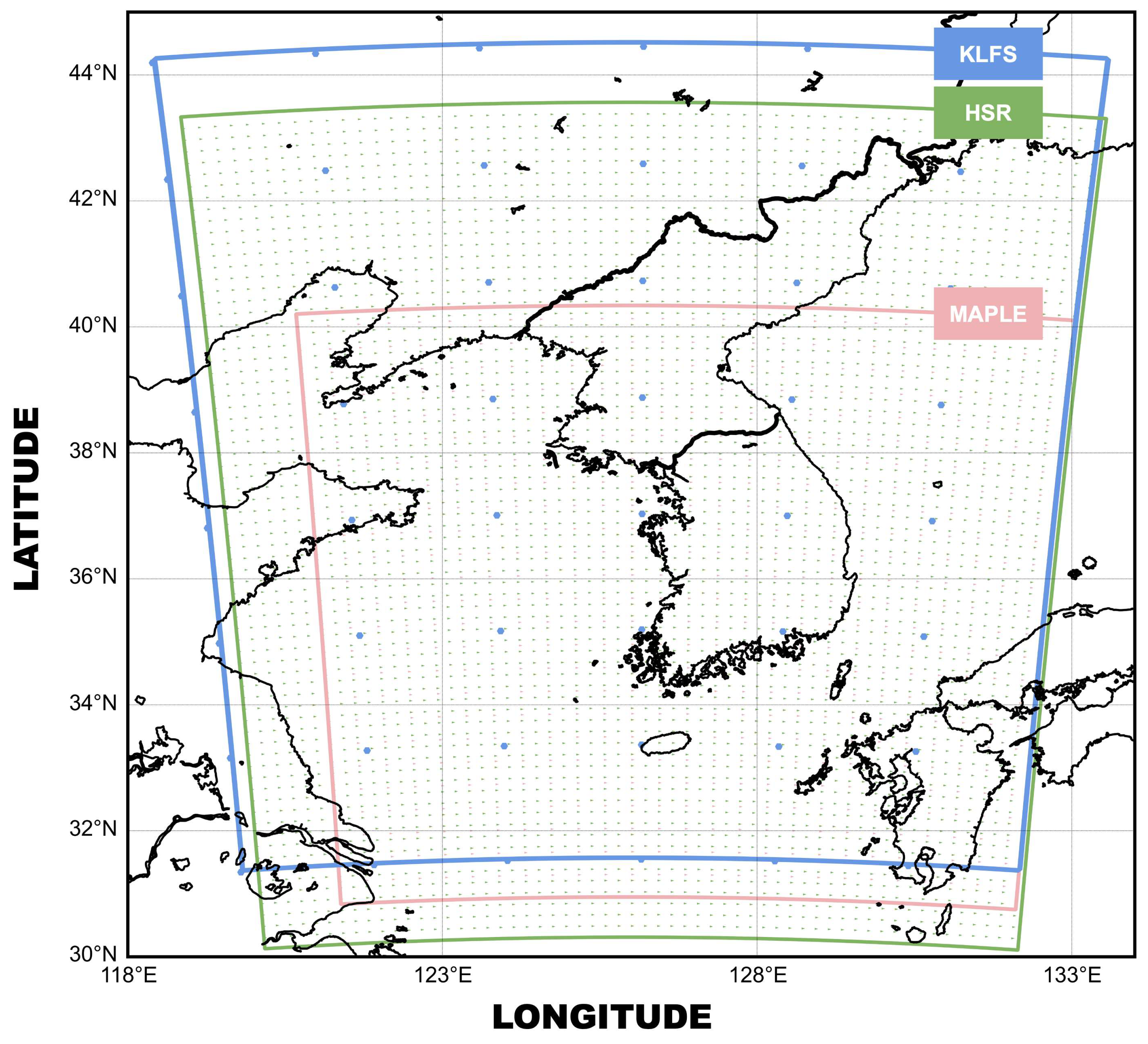
2.1. NWP Model and Radar Observation Data

For precise and prompt rainfall estimation and prediction, radar-based short-term rainfall forecasting is imperative. In this study, three different datasets distributed by the Weather Radar Center of the Korea Meteorological Administration were applied to calculate the temporal weighting function (Figure 1). First, we used MAPLE, originally developed by Bellon and Austin [54] at McGill University in Canada. MAPLE leverages variational echo tracking to calculate the motion vector of the precipitation echo and predicts the position of echoes within a few hours using the semi-Lagrangian method. This method, originally proposed by Laroche and Zawadzki [96], estimates the optimal field of motion vectors as described by Germann and Zawadzki [59] and relies on radar extrapolation data. A detailed examination of VET parameter sensitivity on the motion field is presented in a companion study [97]. For motion vector estimation, MAPLE utilizes three radar composite maps containing maximum reflectivity along the vertical dimension. The model domain encompasses a 1024 (in longitude) × 1024 (in latitude) grid with 1 km horizontal resolution, covering the entire Korean radar network. Echo motion vectors are calculated within sub-areas of 25 × 25 pixels, each representing a 32 km × 32 km region within the larger 800 × 800-pixel sub-domain. To facilitate the semi-Lagrangian advection scheme, bilinear interpolation is applied to the 25 × 25 vector field, generating a velocity vector at each grid point.

Second, we applied KLFS, which is the abbreviation of the Korea Local Analysis and Prediction System (KLAPS), a forecast system. The Korea Local Analysis and Prediction System (KLAPS), developed by NIMS (National Institute of Meteorological Science) in Korea, complements radar-based forecasting by providing a local-scale, high-resolution, and real-time weather data processing and analysis system specific to South Korea. Operational since 2006, KLAPS leverages a fine-grid structure for efficient local analysis. This system functions in two stages: (1) hourly short-range analysis of the current atmospheric state and (2) weather prediction based on the analysis results. In addition to real-time data, KLAPS offers reanalysis data incorporating a wider range of observations and more rigorous analysis, albeit with a time lag of several years for processing and release. KLAPS numerical data are readily available for download in NetCDF format from the Korea Meteorological Administration’s portal (data.kma.go.kr). The model domain encompasses a 235 (in longitude) ± 283 (in latitude) × 40 (in altitude) grid with 5 km horizontal resolution and 50 hPa vertical resolution [98,99,100]. The model employs a terrain-following sigma coordinate system with 40 vertical levels, ranging from 1100 hPa at the lowest level to the upper atmosphere, and contains 46 meteorological parameters including pressure, temperature, wind velocity, specific humidity, etc. [88,101]. To expedite the data assimilation cycle, the Sequential-3DVAR system is employed [102], assimilating only the most recent observations that are valid at or after the analysis time and received within the observation cutoff time, which is 6 min post-analysis [90].

Lastly, we used the HSR approach among different radar data display methods. This approach leverages selective synthesis based on multiple elevation angles, using data acquired closest to the ground surface to mitigate challenges such as precipitation underestimation stemming from terrain echoes, masking effects, and non-precipitation echoes [103,104]. The model domain encompasses a 2305 (in longitude) × 2881 (in latitude) grid with 0.5 km horizontal resolution. To minimize beam blockage, most dual-polarimetric radars in Korea are strategically positioned atop high mountains, reaching elevations of up to 1408 m [92]. This elevated radar placement, however, introduces rainfall estimation errors stemming from the substantial height difference between the radar and the ground. To mitigate this height difference, the scanning strategy incorporates negative elevation angles. Unfortunately, this approach also increases the prevalence of ground clutter, introducing additional challenges for accurate rainfall estimation. To address these challenges, the Hybrid Surface Rainfall (HSR) method effectively mitigates these issues by dynamically adjusting to multiple elevation angles, thereby enhancing the accuracy of rainfall estimation over complex terrains. The HSR method has demonstrated remarkable effectiveness in regions with intricate topographical features, such as Korea, where traditional radar methods often encounter limitations in accuracy. A robust relationship between radar reflectivity and rain rate is also an essential part to quantify the accurate radar rainfall estimation [105,106]. This relationship is commonly quantified through a Z-R power-law equation, as initially proposed by Marshall and Palmer [107]. Radar rainfall retrieval methods primarily depend on spatially and temporally averaged drop size distributions (DSDs), resulting in a fixed Z-R relationship [108,109,110]. In this study, we adopted a relationship between radar reflectivity and rain rate based on the Marshall-Palmer equation ($Z=200R^{1.6}$) [111]. Details of each dataset are presented in

Table 1. Data used in this study.

Dataset	Number of Grids	Spatial Resolution	Temporal Resolution	Forecast Lead Time
MAPLE	1024 × 1024	1 km	10 min	6 h
KLFS	234 × 282	5 km	1 h	12 h
HSR	2305 × 2881	0.5 km	5 min	-

.

To facilitate data integration and comparison, standardization was performed for the number of grids, spatial resolution, and temporal resolution. In terms of spatial resolution, Delaunay triangulation was adopted to unify the number of grids and spatial resolution. This method involves connecting points on a plane to form triangles, aiming to maximizing the minimum angle of each triangle. This strategy is beneficial for clustering data points and has been widely used in various studies, including the generation of 3D polygon meshes [112]. This approach was thus applied to the 2D latitude and longitude data in MAPLE and KLFS. Subsequently, for HSR, which provides the highest spatial resolution of observational data, the Delaunay triangulation triangles corresponding to each grid in the 2D latitude and longitude data of MAPLE and KLFS were identified. The final latitude, longitude, and precipitation data of MAPLE and KLFS were then determined through linear interpolation of the latitude and longitude data at the three vertices of the matched Delaunay triangulation triangles, thus standardizing the spatial resolution. The barycentric coordinates of each new grid point relative to the vertices of the enclosing simplex are computed. Using these barycentric coordinates and the values of the function at the vertices of the enclosing simplex, interpolated values for the grid points are subsequently calculated. Negative recorded values, designated as error values within the dataset, were converted to NaN values, and the data were cropped to focus on the region of interest within the study area. In this study, the southern part of the Korean Peninsula region, ranging from 33.00°N to 39.60°N latitude and 124.00°E to 131.00°E longitude, was selected as the target area for analysis. This area belongs to the UTC (Universal Time Coordinated) +9 zone, and it is denoted as the Local Standard Time (LST).

In terms of temporal resolution, it was deemed that adopting arbitrary interpolation methods could increase variability, considering the aim of optimizing the temporal weighting function in this study. Consequently, hourly data, representing the lowest temporal resolution among the three datasets, were selected and employed for analysis. MAPLE offered 36 datapoints, comprising 6 h rainfall forecasts at 10 min intervals, while KLFS provided 12 datapoints, consisting of 12 h rainfall forecasts at 1 h intervals, for each time point. To maintain consistency across all datasets, we standardized the temporal resolution to the lowest available resolution, which is the 1 h interval provided by the KLFS data. Consequently, only data with a 1 h interval were selected from MAPLE, KLFS, and HSR datasets. Data from MAPLE, KLFS, and HSR were matched for six time steps ranging from 1 to 6 h, predicted relative to a specific time point. Grids with NaN values in both the MAPLE and KLFS datasets were identified, and the corresponding grids in the HSR dataset were set to NaN, while the remaining data were utilized. In this study, three rainfall events were selected with the following details:

(1)

Event 1: 3 August 2020, 00:00 LST to 4 August 2020, 00:00 LST;

(2)

Event 2: 1 August 2021, 00:00 LST to 2 August 2021, 00:00 LST;

(3)

Event 3: 21 August 2021, 00:00 LST to 22 August 2021, 00:00 LST.

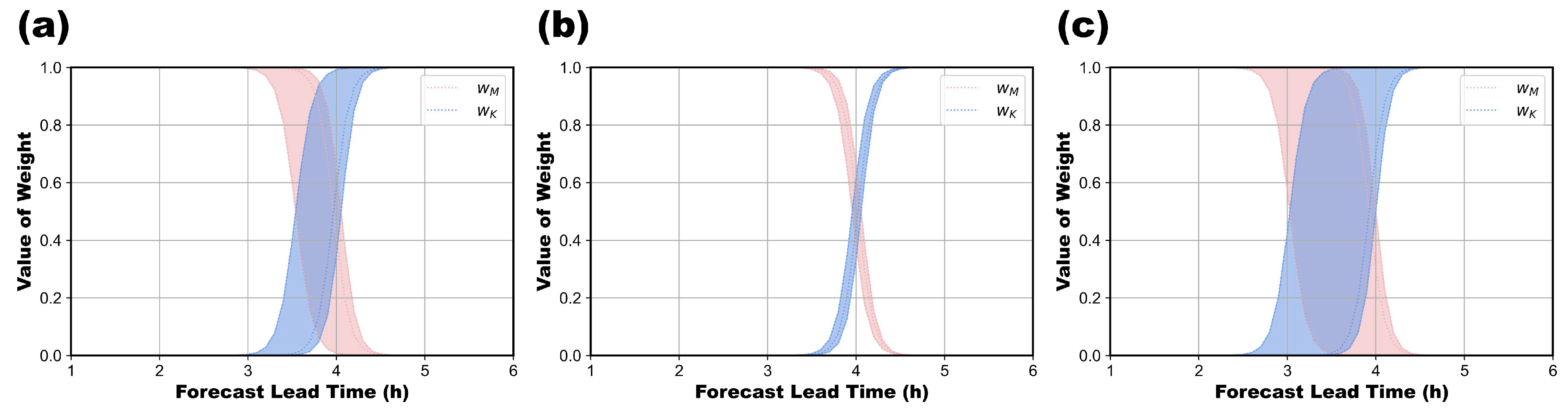
2.2. Temporal Weighting Function

For the nowcasting method described in Section 2.1, the three types of data, which exhibit varying levels of performance, show distinct characteristics in terms of accuracy over time. The predictive accuracy of radar-based extrapolation methods rapidly diminishes within the first several hours of severe weather development due to their inability to account for the growth and decay of storms. As a result, these methods are generally more accurate for short-term forecasts [113,114,115], as illustrated in Figure 2. Conversely, some studies have shown that numerical weather prediction (NWP) models surpass radar-based extrapolation methods over longer time scales by dynamically resolving large-scale atmospheric flow [116,117,118]. In this study, both MAPLE and KLFS include prediction fields but exhibit different characteristics. MAPLE, leveraging a composite radar dataset combined with ground observation station data for calibration, demonstrates high accuracy from the initial forecast lead time up to 3 h [56,75,119,120,121]. Conversely, KLFS, rooted in the characteristics of NWP, performs better beyond the initial hours, which means low skill within the nowcasting range, particularly for areas with complex terrain [59,122,123,124,125]. Merging these datasets with identical weights fails to encapsulate their distinct features.

Consequently, optimal blending strategies could be devised by assigning predominant weight to radar-based datasets (extrapolation forecast) for the initial forecast lead time, while progressively increasing the weights of the NWP dataset as the lead time extends. In this study, we set a forecast lead time of 6 h and performed optimization to derive a temporal weighting function that accurately reflects the characteristics of rainfall data within this period, aiming to achieve superior performance. We attempted to calculate three weighting functions corresponding to the unit forecast lead time (6 h) for all datasets, as defined in Equations (1)–(3). Here, we denote the sine function as SIN, the hyperbolic tangent function as HTN, and the sigmoid function as SIG. The rationale for selecting the weighting schemes of the sine function and hyperbolic tangent function is based on the studies by Yang et al. [127] and Wang et al. [128]. They compared these three weighting schemes including real-time scrolling weight and found that merging results using the hyperbolic tangent curve weight were closer to observations. In the case of the sigmoid function, it is widely utilized in fields such as machine learning [129], statistics [130], and signal processing [131]. It was chosen as a weighting scheme in this study due to its ability to provide smooth and continuous transitions between values, allowing for a gradual reflection of dataset influences over time. Moreover, the nonlinear nature of the sigmoid function is beneficial for modeling complex relationships between variables, facilitating the flexible representation of nonlinear interactions between datasets. The parameters for each function are represented by $a$ and $b$. The parameter $a$ primarily serves as a scaling factor for the input variable $t$, affecting the rate of change or steepness of the function. The parameter $b$ functions as a translation factor, shifting the graph of the function horizontally along the $t$-axis.

$$SIN={\sin }^2 (a\ast t-b)$$

(1)

$$HTN={\displaystyle \frac{1+\mathrm{t}\mathrm{a}\mathrm{n}\mathrm{h} (\mathrm{a}\ast \left(\mathrm{t}-\mathrm{b}\right))}{2}}$$

(2)

$$SIG={\displaystyle \frac{1}{1+e^{-a\ast (t-b)}}}$$

(3)

The SIN function [Equation (1)] is emblematic of periodic variations and is suited for modeling phenomena characterized by regular, cyclic behavior. The parameter $a$ modulates the frequency of oscillations, thereby dictating the rate of cycle repetition, while $b$ adjusts the phase, setting the initial point of the cycle. For physical application, the SIN function is well-suited for modeling periodic hydrological and meteorological phenomena such as seasonal rainfall patterns, tidal cycles, and temperature variations. The HTN function [Equation (2)] is depicting a smooth, sigmoidal transition between states, effectively capturing nonlinear, gradual changes. The parameter $a$ influences the steepness of the transition, indicating the rapidity of the change, while $b$ shifts the transition point along the time axis. For physical applications, the HTN function effectively captures smooth, sigmoidal transitions, making it suitable for representing processes that undergo gradual, nonlinear changes such as snowmelt processes, water table fluctuations, and atmospheric fronts. The SIG function [Equation (3)] is the logistic function model, which is suitable for capturing gradual, asymptotic changes, typically used for systems that initiate slowly, change rapidly, and then level off. The parameter $a$ dictates the steepness of the curve, whereas $b$ controls the midpoint of the transition. For physical applications, the SIG function could be applied to model flood hydrographs, soil moisture dynamics, and adoption of climate technologies.

To enhance the accuracy of rainfall data through the blending of two datasets, we conducted extensive experiments on bound conditions and constraint functions to derive the optimal temporal weighting function via optimization process. For this reason, we set bound conditions to ensure the half-period of the temporal weighting function fell within a forecast lead time of 1 to 6 h. Additionally, we formulated constraint functions, such as specifying the value of $W_{NWP}$ at specific time points (e.g., $W_{NWP}=1$ when $t=6 \mathrm{h}$). Excluding results that yielded temporal weighting function with linear relationship, three conditions that produced efficient optimization results were selected: (1) The initial estimates for both a and b were set as 0. (2) The difference between $W_{NWP}$ at t = 1 h and t = 6 h was set as 1. (3) NaN values were replaced with 0 to facilitate computation. These conditions were then applied to the entire dataset to carry out the optimization process based on the Equation (4). This methodology enables the identification of data exerting significant influence on the blending process at specific temporal instances, thereby facilitating the detection of outliers deviating from established functional relationships.

$$Minimize [{\left(1-W_{NWP}\right)\ast R_{MAPLE}+W}_{NWP}\ast R_{KLFS}-R_{HSR}]$$

(4)

In Equation (4), $W$ and $R$ represent the weighting function and rainfall data (unit: mm/h) within the dataset, respectively, with subscripts denoting the dataset name. Lastly, verification of $W_{NWP}$ was conducted. For all data within rainfall events, steps (1), (2), and (3) were iteratively performed to determine the values of a and b and confirm the function form. The parameters (a, b) of the weighting function were validated based on the values corresponding to Q1 (25%), Q2 (50%), and Q3 (75%) of the data distribution.

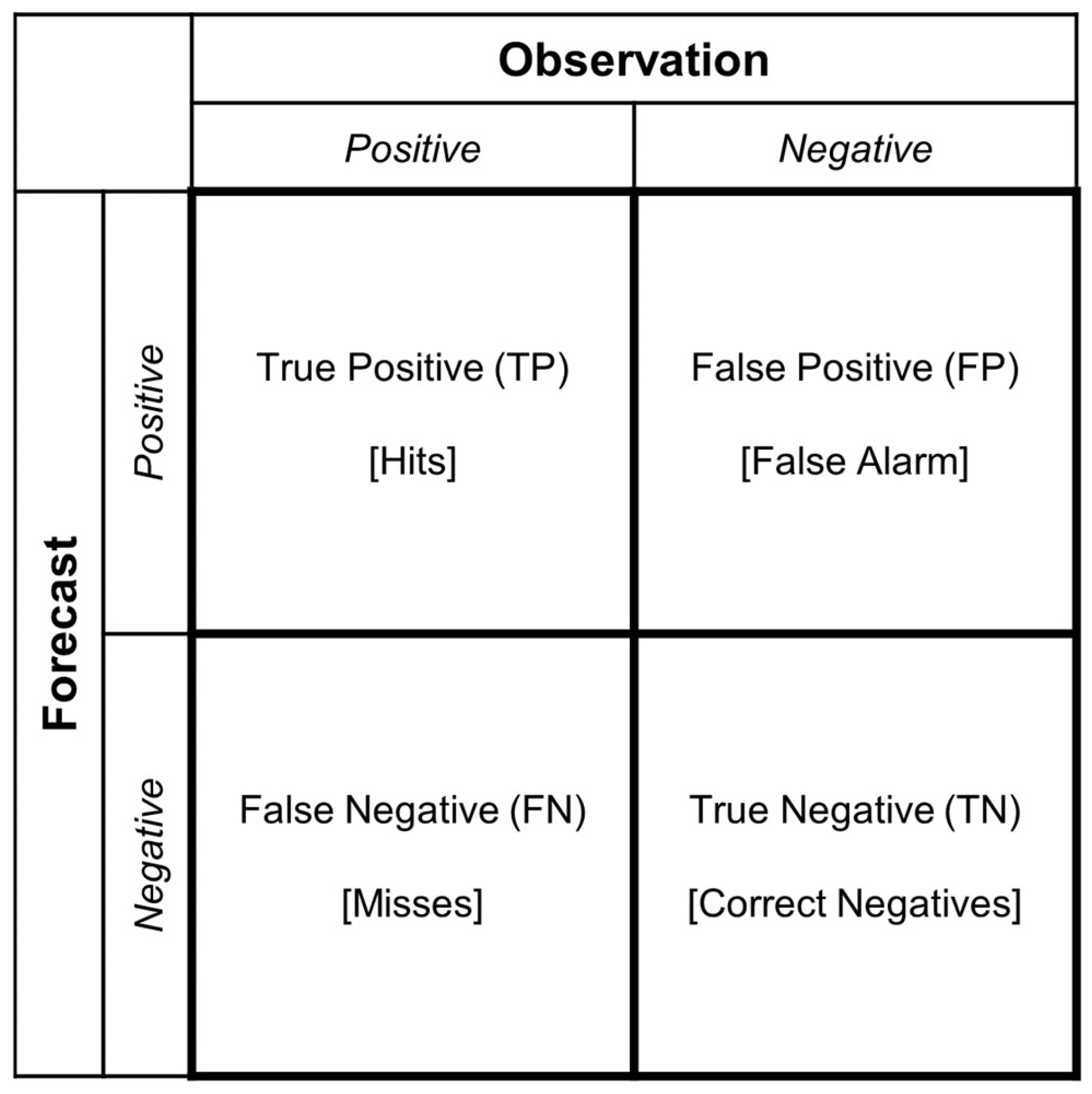
2.3. Performance Index

The performances of the radar-based extrapolation model, NWP model, bias-corrected scheme, and merged forecast were qualitatively evaluated through pattern matching using performance indices based on the contingency table. In the meteorological domain, quantitative assessment is typically conducted using evaluation indices calculated based on the contingency table [132], which is advantageous to understand dichotomous forecasts [133]. Contingency-table-based metrics are indispensable tools for evaluating forecast performance in hydrology and meteorology [134,135]. These metrics provide a granular assessment of forecast accuracy, encompassing hit rates, false alarms, misses, and correct negatives [136]. Such detailed analysis empowers researchers and practitioners to comprehensively understand the strengths and weaknesses of predictive models, thereby enhancing forecast reliability [137]. Consequently, informed decision-making is facilitated for a range of applications, including weather-related emergencies and water resource management. By systematically employing these metrics, meteorologists and hydrologists can optimize model selection and calibration, ultimately contributing to more accurate and dependable forecasts [138,139].

The most prevalent type of contingency table is the 2 × 2 table, which evaluates dichotomous variables (Figure 3). In this table, True Positive (TP) indicates the detection of events via both the reference observation and simulation, while False Negative (FN) represents events identified via the reference observation but overlooked with the simulation. False Positive (FP), also referred to as a false alarm, signifies events identified via the simulation but not confirmed with observations. True Negative (TN) represents the number of instances where the model correctly predicted the absence of a condition or event. To calculate the contingency table, the threshold of rainfall to define hit or not was set at 10 mm/h, which is similar to the resolution of the tipping bucket rain gauge, set at 0.1 mm/min [140,141,142]. Various metrics can be defined based on the contingency table [138,143]:

$$Probability of Detection \left(POD\right)={\displaystyle \frac{TP}{(TP+FN)}}$$

(5)

$$False Alarm Ratio \left(FAR\right)={\displaystyle \frac{FP}{(FP+TP)}}$$

(6)

$$Critical Success Index (CSI)={\displaystyle \frac{TP}{(TP+FP+FN)}}$$

(7)

$$True Positive Rate (TPR)={\displaystyle \frac{TP}{(FN+TP)}}$$

(8)

$$False Positive Rate (FPR)={\displaystyle \frac{FP}{(FP+TN)}}$$

(9)

$$Root Mean Squared Error (RMSE)=\sqrt{{\displaystyle \frac{{\sum }_{i=1}^N{‖y\left(i\right)-\widehat{y}\left(i\right)‖}^2}{N}}}$$

(10)

(1)

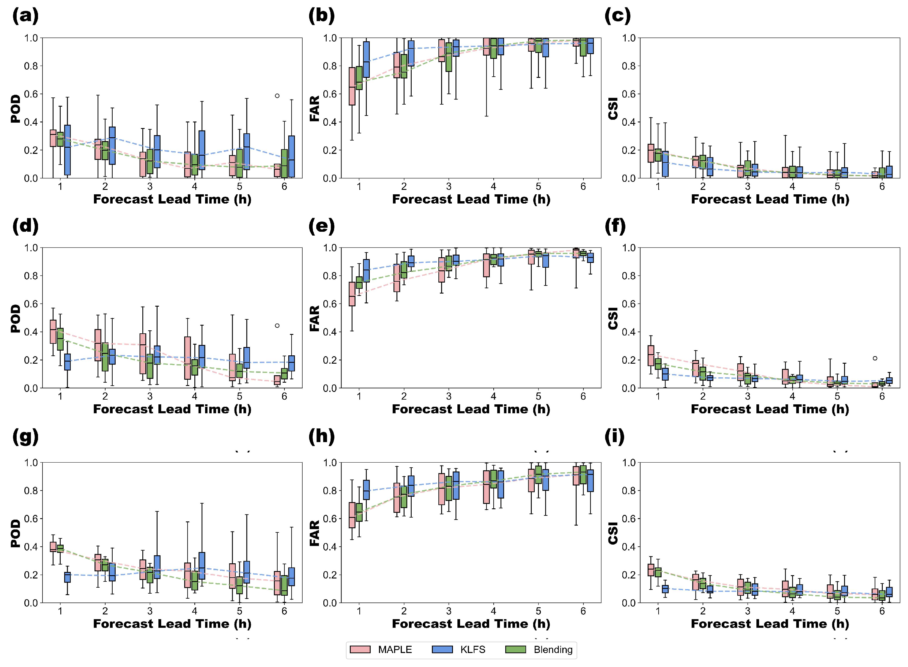
Probability of Detection (POD) quantifies the proportion of reference observations correctly identified via the simulation. It can be calculated using Equation (5), with values ranging from 0 to 1, with 0 denoting no skill, while 1 represents a perfect score;

(2)

False Alarm Ratio (FAR) indicates the fraction of events identified via the simulation but not confirmed with reference observations. It can be calculated using Equation (6), with values ranging from 0 to 1, with 0 denoting a perfect score;

(3)

Critical Success Index (CSI), also referred to as the Threat Score, integrates various aspects of POD and FAR, providing an overall assessment of the simulation performance relative to reference observation. It can be calculated using Equation (7), with values ranging from 0 to 1, with 0 indicating no skill, while 1 signifies a perfect score;

(4)

True Positive Rate (TPR), also known as Sensitivity or Recall, represents the proportion of positive events correctly identified via the simulation among all actual positive events. It can be calculated using Equation (8), with values ranging from 0 to 1, with 0 indicating no true positives detected, while 1 denotes perfect identification of positive events;

(5)

False Positive Rate (FPR), also referred to as the Fall-out, quantifies the fraction of negative events incorrectly identified as positive via the simulation out of all actual negative events. It can be computed using Equation (9), with values ranging from 0 to 1, with 0 denoting a perfect score, indicating no false positives, while 1 signifies all negative events being falsely identified as positive;

(6)

Root Mean Squared Error (RMSE) measures the average magnitude of errors between predicted and observed values, indicating the model performance in capturing the data variability. It is computed using Equation (10), where N represents the total number of observations, $\widehat{y}\left(i\right)$ denotes the predicted value, and $y\left(i\right)$ represents the observed value for the ith observation. The RMSE ranges from 0 to positive infinity, with lower values indicating better model performance.

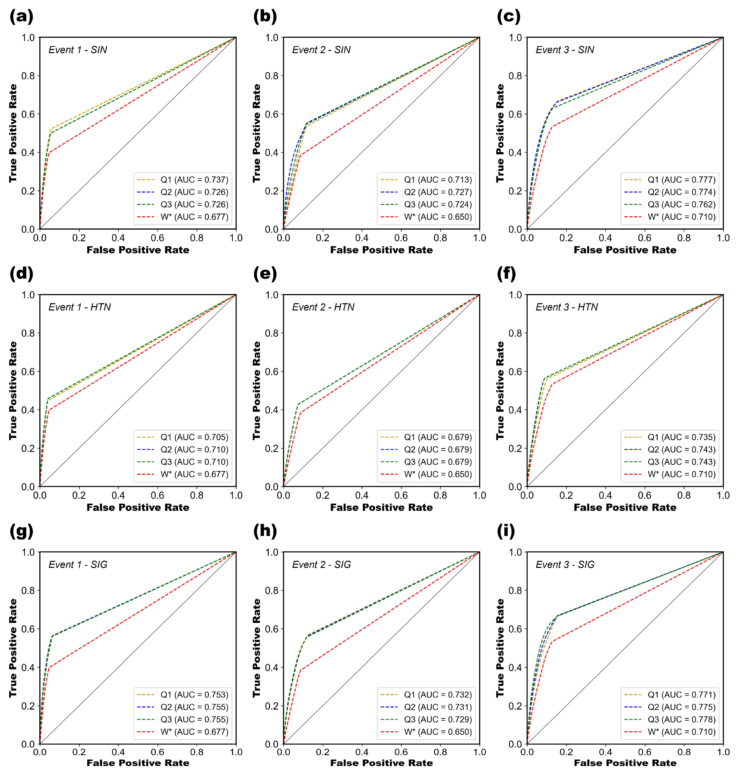
2.4. Receiver Operating Characteristic (ROC) Curve

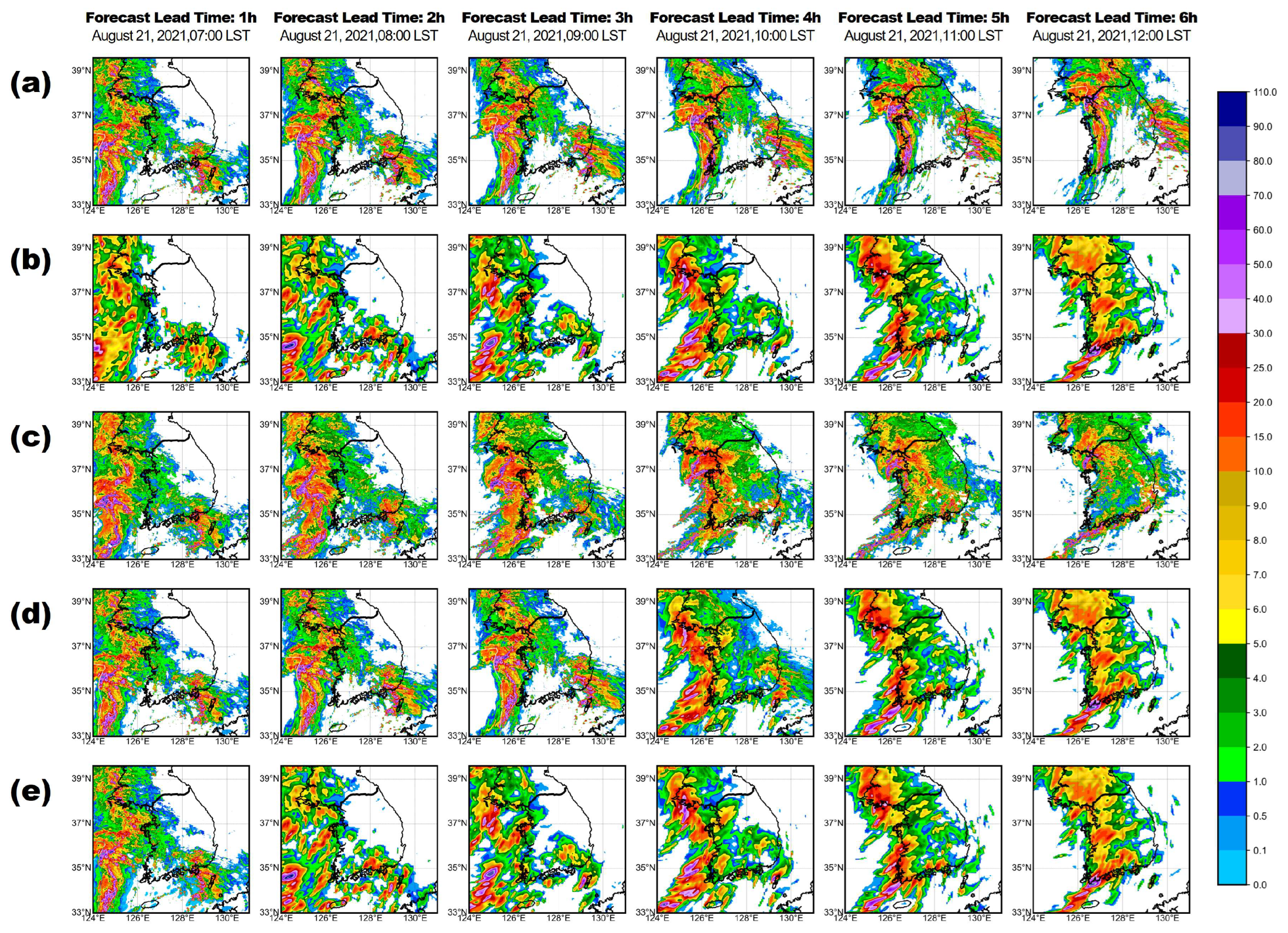
The ROC curve is a graphical representation of the FPR on the x-axis and TPR on the y-axis for varying cut-off points of test values. It is typically depicted within a square box for ease of visualization, with both axes ranging from 0 to 1. The area under the curve (AUC) serves as a comprehensive metric for assessing the intrinsic validity of a precipitation detection validation, combining sensitivity and specificity. An AUC value of 1 indicates flawless differentiation between detection and non-detection of precipitation, where TPR is 0 and FPR is 1 or TPR is 1 and FPR is 0. However, such ideal conditions are exceedingly rare in practical settings due to overlapping distributions of detection and non-detection of precipitation validation values. Consequently, the AUC is used to numerically compare model performance, providing a quantitative assessment of performance.

3. Results

3.1. Performance Results of Temporal Weighting Function

3.1.1. Parameter Results across Different Quartiles

Three types of temporal weighting functions (SIN, HTN, and SIG) with three distinct rainfall events (Events 1, 2, and 3) were combined to ascertain the parameters within each function. The entire event was segmented into 6 h unit forecast lead times, for which parameters were derived individually. Subsequently, these parameters were combined to characterize the temporal weighting function for each event. The concatenated dataset was sorted in ascending order and divided into quartiles. Values corresponding to the 25th, 50th, and 75th percentiles (Q1, Q2, and Q3) were computed for each quartile and presented in

Table 2. Parameter quartiles based on combined weighting functions and rainfall events.

Weight Function	Rainfall Event	Parameter Quartile
		Q1 (25%)		Q2 (50%)		Q3 (75%)
		a	b	a	b	a	b
SIN	Event 1	−0.314	2.827	0.314	14.451	0.314	96.133
	Event 2	−0.314	0.340	0.031	16.000	0.314	64.560
	Event 3	0.185	0.000	0.314	7.728	0.314	16.022
HTN	Event 1	5.221	3.539	5.565	3.968	5.949	4.053
	Event 2	5.501	3.957	5.689	4.020	6.024	4.059
	Event 3	5.332	3.028	5.667	3.924	6.156	4.000
SIG	Event 1	1.000	3.572	1.000	4.650	1.000	5.602
	Event 2	1.000	4.757	1.000	5.475	1.000	5.982
	Event 3	1.000	2.885	1.000	3.696	1.000	4.833

. In order to highlight the event-specific variability in the optimized parameters of the temporal weighting functions, the HTN function was selected, and the results are graphically presented in Figure 4. The extent of variation in the x-axis values of the plotted functions exhibited a clear pattern. Event 3 showed the greatest variability, followed by Event 1 and Event 2. This finding is consistent with the level of fluctuation in rainfall intensity over the 6 h period, as depicted in Section 3.2.

3.1.2. Comparison of Performance Results with Previous Studies

The performance of the proposed temporal weighting functions was evaluated through a comparison with an existing weighting function scheme from a previous study [80]. A previous study, through sensitivity analyses, established optimal parameter values for the hyperbolic tangent curve weight (HTW) method based on event types: supercell (a = 7, b = 1.5), line (a = 11, b = 0.25), and multicell (a = 15, b = 0.166). For comparative purposes, the parameters associated with the multicell type were utilized in this study, given the multicell nature of the events under consideration.

On the ROC curve, results obtained using the weighting function proposed by Radhakrishnan and Chandrasekar [80] (denoted by W*) in Figure 5 were compared. Additionally, Figure 5 shows the results for three types of temporal weighting functions (SIN, HTN, and SIG), three events (Events 1–3) and three quartiles of the weighting function parameter (Q1, Q2, and Q3). In all cases, the AUC derived from the application of W* exhibited lower values compared with those obtained through parameters optimized in this study. Notably, among all weighting functions, the SIG function displayed the most significant disparity (average difference in AUC = 0.076), while the HTN weighting function demonstrated the least deviation (average difference in AUC = 0.029).

3.2. Blending Results with Performance Index

The accuracy of the proposed weighting functions was assessed using the proposed metrics of POD, FAR, and CSI. Most verification schemes are conducted using threshold-based categories, and we have selected 10 mm/h as the threshold for defining rainfall existence. It is a standard threshold used to differentiate light rainfall and moderate rainfall [144,145]. In this study, the datasets MAPLE, KLFS, and HSR were binarized by setting grids exceeding the threshold to 1 and the remaining grids to 0. The binarized HSR data were used as the true values, and contingency tables were computed for each of the binarized MAPLE and KLFS datasets. Based on these contingency tables, the values for POD, FAR, and CSI were calculated according to Equations (5)–(7).

The HTN weighting function was selected due to its minimal deviation across all rainfall events based on the result from Section 3.1.2, and the analyzed results (Figure 6) are as follows: First, we explore the results of POD. From the initial forecast lead time up to 3 h, MAPLE exhibited higher accuracy than Blending, but beyond 3 h, the accuracy trend reversed. Similarly, for KLFS, a lower accuracy compared with Blending was observed from the initial forecast lead time up to 2–3 h, with a reversed trend noted beyond this forecast lead time. For FAR, consistent outcomes were observed across all events. From the initial forecast lead time up to 3 h, MAPLE, Blending, and KLFS showed higher accuracy, in that order. However, for forecast lead times beyond 3 h, the application of the proposed weighting functions resulted in the lowest accuracy in the order of MAPLE, KLFS, and Blending. Lastly, the results of CSI mirrored those of FAR in terms of accuracy ranking.

Overall, as the threshold increases, the frequency of events decreases, exacerbating the impact of prediction errors and potentially degrading performance metrics. When the threshold is set at 1 mm/h, which is typically used to distinguish light rainfall, the overall frequency of events increases, resulting in higher metric values. However, in this study, to consider extreme rainstorm events, we set the threshold at 10 mm/h, corresponding to moderate rainfall. This resulted in deficient metric values compared to general standards. Furthermore, the datasets used in this study were analyzed without temporal or spatial aggregation, distinguishing rainfall occurrence at the available temporal resolution (1 h) and the most granular spatial resolution (0.5 km). These findings illustrate the inherent challenges in predicting extreme weather phenomena and indicate the necessity of future research which is able to focus on diversifying thresholds to achieve higher accuracy in various spatiotemporal condition of rainfall [146]. Nevertheless, it is noteworthy that the blending results still demonstrated better performance than the prediction data currently in use, underscoring the effectiveness of the proposed method.

Furthermore, the prediction accuracy was quantitatively assessed using the RMSE. Here, $\widehat{y}\left(i\right)$ denoted HSR, and $y\left(i\right)$ corresponded to Blending, W*, KLFS, and MAPLE to calculate the RMSE.

Table 3. RMSE results for different combinations of rainfall event, data type, and forecast lead time.

Rainfall Event	Data Type	Forecast Lead Time
		1 h	2 h	3 h	4 h	5 h	6 h
Event 1	Blending	12.064	14.915	14.231	13.283	12.687	12.329
	W*	11.431	13.881	14.608	13.864	14.798	14.703
	KLFS	12.623	14.078	14.925	14.345	14.901	15.234
	MAPLE	11.869	13.457	13.723	14.867	14.590	15.205
Event 2	Blending	11.436	14.299	12.126	12.043	11.638	13.770
	W*	11.944	14.466	15.552	11.790	13.388	13.220
	KLFS	12.554	14.706	16.319	15.207	15.078	14.210
	MAPLE	12.428	13.414	14.654	15.332	15.561	15.132
Event 3	Blending	11.436	14.299	12.126	12.043	11.638	13.770
	W*	11.362	15.565	15.609	14.083	12.052	16.539
	KLFS	11.981	14.581	14.966	14.169	15.053	14.745
	MAPLE	12.057	14.449	15.446	15.558	15.139	14.764
Total	Blending	11.524	14.885	13.788	12.974	12.052	12.974
	W*	11.838	14.413	14.932	13.864	14.232	14.703
	KLFS	12.323	14.525	15.523	15.094	15.028	14.764
	MAPLE	12.033	14.001	14.324	15.197	15.249	15.286

presents the median values of RMSE for each event and the overall events based on forecast lead time. In Event 1, RMSE values indicated that W* yielded the least accurate results at a forecast lead time of 1 h, while MAPLE performed best at 2 and 3 h. Blending exhibited the lowest RMSE beyond a forecast lead time of 3 h. In Event 2, Blending achieved the lowest RMSE at 1 h, MAPLE at 2 h, and, alternatingly, Blending and W* at subsequent forecast lead times. In Event 3, Blending results achieved the lowest RMSE across all time points except at a forecast lead time of 1 h. Overall, Blending consistently demonstrated the lowest RMSE across all time points except at a forecast lead time of 2 h. At this time point, the lowest RMSE was observed in the MAPLE data, which showed a difference of 0.884 compared to the blending results. For the 1 h forecast lead time, the KLFS model outperformed the blended results by reducing the RMSE by 0.799. However, for the 4–6 h forecast lead times, the MAPLE data demonstrated a substantial improvement of 2.295 in RMSE, particularly addressing the limitations of long-term forecasting.

To evaluate the prediction accuracy, the results for MAPLE, KLFS, HSR, and Blending were concurrently plotted, with representative cases for each event depicted in Figure 7, Figure 8 and Figure 9. The horizontal axis of these figures represents the forecast lead time, comprising six columns (1–6 h), while the vertical axis denotes the data types, featuring five rows (MAPLE, KLFS, HSR, Blending, and W*). The reference times for Events 1, 2, and 3 were set as 3 August 2020, 09:00 LST; 1 August 2021, 11:00 LST; and 21 August 2021, 06:00 LST, respectively. Across all events, MAPLE exhibited higher accuracy within 3 h, while KLFS demonstrated higher accuracy thereafter. Conversely, Blending consistently showed high accuracy regardless of forecast lead time, indicating its effectiveness compared with conventional methods that heavily rely on rainfall cell generation and dissipation criteria.

4. Discussion

In this study, a temporal weighting function was optimized to blend two types of forecast datasets, using radar observation data as the target. The results derived from blending using a temporal weighting function appropriate for the forecast lead time highlight the efficacy of the time-weighted functions specifically designed for each rainfall event and forecast lead time. This method offers a significant improvement over traditional approaches that rely on broad classification criteria based on rainfall type. Additionally, the temporal weighting function, derived with minimal computational resources, demonstrated substantial value by efficiently estimating rapidly changing rainfall events through a simple yet effective weighting function algorithm. While promising results are yielded in this study, it is essential to address numerous limitations to broaden the applicability of the proposed algorithm.

First, a uniform temporal weighting function was applied across the entire study area. The proposed methodology may be limited by its inability to fully account for the diverse climatic and geographic conditions within the study area. Rainfall patterns are significantly influenced by factors such as topography, land use, and localized weather systems, which can vary substantially across different regions. For instance, mountainous and coastal areas often exhibit distinct rainfall characteristics. In mountainous regions, rainfall is often influenced by orographic lifting, where moist air is forced to ascend over mountain ranges, leading to enhanced precipitation. A uniform weighting function that disregards the significant local characteristics within the study area might not adequately represent the increased rainfall rates in such areas, resulting in underestimation or misrepresentation of actual rainfall events. Additionally, in urban areas, unique rainfall characteristics emerge due to the combined effects of the urban heat island and increased surface runoff, often leading to more intense but shorter precipitation events. Consequently, a uniform weighting function may inadequately capture these localized extremes, potentially underestimating flood risks.

Second, as the forecast lead time increases, the dependence on numerical weather prediction (NWP) models becomes more significant. For this study, the forecast lead time for blending was set to 6 h, and it was observed that all three weighting functions assigned a weight of 1 to the NWP for forecast lead times after 6 h. One of the critical limitations associated with longer forecast lead times is the degradation in spatial resolution. Among the three types of data used in this study, the NWP data has the longest forecast lead time but the lowest spatial resolution. This reduction in resolution can hinder the model’s ability to accurately capture fine-scale rainfall features such as localized convective storms, topographic influences, and small-scale weather phenomena. High-resolution details which are crucial for precise rainfall predictions in areas with complex terrain or varying land-use patterns must be considered potentially.

Lastly, the temporal weighting function was predefined in its form prior to the optimization process. Although this approach allows for a structured and controlled optimization procedure, it could affect the flexibility and adaptability of the model in various meteorological scenarios. As a result, the optimized function may not be the most suitable for all scenarios, potentially leading to suboptimal performance in cases that deviate significantly from the assumed structure. When attempting to capture rapid changes in short forecast lead times, a predefined functional form may fail to quickly reflect sudden changes in rainfall intensity and distribution. This lack of adaptability can result in less accurate forecasts and reduced capability to predict extreme weather events.

Future research should investigate the potential of machine learning techniques to optimize the fusion of numerical weather prediction (NWP) and radar-based extrapolation prediction data. By capitalizing on the strengths of both data sources, machine learning models can be trained to dynamically adjust weighting functions based on real-time atmospheric conditions. This approach necessitates the integration of advanced algorithms, such as deep learning, ensemble methods, and reinforcement learning, to effectively learn from historical data and refine the blending process iteratively. To enhance model accuracy and reliability, it is crucial to incorporate physical atmospheric characteristics, including but not limited to pressure, temperature, humidity, wind speed, and direction, into the feature engineering process. Furthermore, the adoption of physics-informed neural networks (PINNs) can ensure adherence to fundamental physical laws. By embedding physical constraints within the machine learning framework, the derived temporal weighting functions can more accurately represent real-world meteorological conditions. To further improve predictive accuracy, the assimilation of high-resolution observational data and advancements in data assimilation techniques are essential. Ultimately, these machine learning-based frameworks offer the potential to reconcile the short-term strengths of radar-based extrapolation with the long-term reliability of NWP models, thereby advancing severe weather forecasting and disaster management.

Furthermore, methodologies that enable blending over a wider range of temporal units should be explored. In this study, blending was conducted using six time points at 1 h intervals as the unit forecast lead time, combining data into a single dataset for each corresponding time point. This approach, while effective, presents certain limitations in assessing the broader impact of different temporal scales on prediction accuracy. To address these limitations and enhance predictive capabilities, future studies should investigate the application of a time-lagged ensemble approach for blending. A time-lagged ensemble blending method involves incorporating forecasts from different lead times into a single predictive model, thereby taking advantage of the strengths of each forecast’s temporal specificity and mitigating the weaknesses inherent in individual forecast lead times. By integrating forecasts made at various times before the target event, the model can better capture the temporal evolution of weather phenomena and improve overall predictive accuracy. The implementation of this method involves several steps: collecting and standardizing forecast data from multiple lead times, extracting relevant features that accurately represent the physical processes, developing advanced machine learning models that dynamically adjust weighting based on predictive performance, optimizing and validating the model with historical data, and applying it in real-time scenarios. By adopting a time-lagged ensemble approach, future research can develop more sophisticated blending techniques that reflect the different characteristics of independent-time-scale data.

5. Conclusions

In this research, we tackled the challenge of temporal resolution in rainfall data and reduced computational complexities by improving rainfall prediction accuracy through the integration of radar-based extrapolation techniques with numerical weather prediction (NWP) models. The main goal was accomplished by optimizing a temporal weighting function. We employed two types of forecast data: the McGill Algorithm for Precipitation Nowcasting by Lagrangian Extrapolation (MAPLE) and the Korea Local Analysis and Prediction System (KLAPS), while using Hybrid Surface Rainfall (HSR) as the target data for the radar-based extrapolation method. The temporal weighting function was designed to adjust to varying weights depending on the lead time of forecast data, and we implemented three distinct types of temporal weighting functions (SIN, HTN, and SIG). Each event was divided into unit forecast lead time (6 h), and parameters were derived. The total dataset was sorted and divided into quartiles, with values for the 25th, 50th, and 75th percentiles. Subsequently, we analyzed the deviations of the temporal weighting functions based on the calculated parameters. Additionally, we compared the blending results obtained from a previous study, which employed event-type-based weighting functions, with the results from our proposed methodology using temporal weighting functions, utilizing performance indices derived from a contingency table and a quantitative metric.

Using the HTN function, one of the temporal weighting functions, results were graphically presented by ROC curve to illustrate event-specific variability, and it was observed that the variability in the optimized parameters closely mirrored the variability in the rainfall events, indicating a consistent pattern between the two. Furthermore, all three types of temporal weighting functions consistently exhibited superior performance compared with the function proposed in prior work, displaying higher AUC values across all combinations of weighting functions and rainfall events. Notably, the SIG function displayed the most significant deviation, averaging an AUC of 0.076, while the HTN function exhibited the least deviation with an average AUC of 0.029. Subsequently, we compared the results from MAPLE and KLFS with the blending results obtained using the temporal weighting function proposed in this study, as well as the blending results based on the weighting function from previous studies. Based on the performance evaluation using POD, FAR, and CSI values, the blending results demonstrated superior performance at both the early (1 h–3 h) and later (4 h–6 h) forecast lead times, where MAPLE and KLFS each showed limitations. Specifically, blending results exhibited superior metrics at all forecast lead times, except at 2 h, in terms of the RMSE for the entire rainfall event. The MAPLE data exhibited the lowest RMSE at this time point, differing by 0.884 from the blended results. For the 1 h forecast lead time, KLFS demonstrated an improvement of 0.799 in the RMSE compared with the blending results. Conversely, for the 4–6 h forecast lead times, MAPLE data from the radar extrapolation approach exhibited an average improvement of 2.295 in RMSE, addressing the shortcomings observed in long-term forecasting.

The proposed blending method based on temporal weighting functions can account for the temporal characteristics of different forecast data at unit forecast lead times, significantly reducing computational resources while overcoming the temporal limitations of existing forecast data. By considering a broader spectrum of temporal scales, this method enhances rainfall prediction accuracy, thereby improving preparedness for associated hazards such as flooding, landslides, and infrastructure damage. Future research should explore the integration of machine learning for temporal weight optimization and the development of more generalized blending techniques across diverse rainfall event types.

References

1. Arnell, N.W.; Lowe, J.A.; Challinor, A.J.; Osborn, T.J. Global and Regional Impacts of Climate Change at Different Levels of Global Temperature Increase. Clim. Chang. 2019, 155, 377–391. [Google Scholar] [CrossRef]
2. Lindsey, R.; Dahlman, L. Climate Change: Global Temperature. Climate.gov 2020, 16. Available online: https://www.climate.gov/news-features/understanding-climate/climate-change-global-temperature (accessed on 5 August 2024).
3. Crowley, T.J. Causes of Climate Change over the Past 1000 Years. Science 2000, 289, 270–277. [Google Scholar] [CrossRef] [PubMed]
4. Etukudoh, E.A.; Ilojianya, V.I.; Ayorinde, O.B.; Daudu, C.D.; Adefemi, A.; Hamdan, A. Review of Climate Change Impact on Water Availability in the USA and Africa. Int. J. Sci. Res. Arch. 2024, 11, 942–951. [Google Scholar] [CrossRef]
5. Radha, S.V.V.D.; Sabarathinam, C.; Al Otaibi, F.; Al-Sabti, B.T. Variation of Centennial Precipitation Patterns in Kuwait and Their Relation to Climate Change. Environ. Monit. Assess. 2023, 195, 20. [Google Scholar] [CrossRef] [PubMed]
6. Rahmani, F.; Fattahi, M.H. Climate Change-Induced Influences on the Nonlinear Dynamic Patterns of Precipitation and Temperatures (Case Study: Central England). Theor. Appl. Climatol. 2023, 152, 1147–1158. [Google Scholar] [CrossRef]
7. Bindoff, N.L.; Willebrand, J.; Artale, V.; Cazenave, A.; Gregory, J.M.; Gulev, S.; Hanawa, K.; Le Quere, C.; Levitus, S.; Nojiri, Y. Observations: Oceanic Climate Change and Sea Level. 2007. Available online: https://nora.nerc.ac.uk/id/eprint/15400/ (accessed on 5 August 2024).
8. Nerem, R.S.; Beckley, B.D.; Fasullo, J.T.; Hamlington, B.D.; Masters, D.; Mitchum, G.T. Climate-Change–Driven Accelerated Sea-Level Rise Detected in the Altimeter Era. Proc. Natl. Acad. Sci. USA 2018, 115, 2022–2025. [Google Scholar] [CrossRef] [PubMed]
9. Roy, P.; Pal, S.C.; Chakrabortty, R.; Chowdhuri, I.; Saha, A.; Shit, M. Effects of Climate Change and Sea-Level Rise on Coastal Habitat: Vulnerability Assessment, Adaptation Strategies and Policy Recommendations. J. Environ. Manag. 2023, 330, 117187. [Google Scholar] [CrossRef] [PubMed]
10. Yum, S.-G.; Song, M.-S.; Adhikari, M. Das Assessing Typhoon Soulik-Induced Morphodynamics over the Mokpo Coastal Region in South Korea Based on a Geospatial Approach. Nat. Hazards Earth Syst. Sci. 2023, 23, 2449–2474. [Google Scholar] [CrossRef]
11. Om, K.; Ren, G.; Jong, S.; Ham, Y.; Hong, C.; Kang-Chol, O.; Tysa, S.K. Spatial and Temporal Patterns in Observed Extreme Precipitation Change over Northern Part of the Korean Peninsula. J. Geophys. Res. Atmos. 2024, 129, e2023JD039305. [Google Scholar] [CrossRef]
12. Lee, M.; Min, S.-K.; Cha, D.-H. Convection-Permitting Simulations Reveal Expanded Rainfall Extremes of Tropical Cyclones Affecting South Korea due to Anthropogenic Warming. npj Clim. Atmos. Sci. 2023, 6, 176. [Google Scholar] [CrossRef]
13. Waqas, M.; Humphries, U.W.; Hlaing, P.T.; Wangwongchai, A.; Dechpichai, P. Advancements in Daily Precipitation Forecasting: A Deep Dive into Daily Precipitation Forecasting Hybrid Methods in the Tropical Climate of Thailand. MethodsX 2024, 12, 102757. [Google Scholar] [CrossRef]
14. Bansal, K.; Tripathi, A.K.; Pandey, A.C.; Sharma, V. RfGanNet: An Efficient Rainfall Prediction Method for India and Its Clustered Regions Using RfGan and Deep Convolutional Neural Networks. Expert Syst. Appl. 2024, 235, 121191. [Google Scholar] [CrossRef]
15. Anuradha, T.; Formal, P.S.G.A.S.; RamaDevi, J. Hybrid Model for Rainfall Prediction with Statistical and Technical Indicator Feature Set. Expert Syst. Appl. 2024, 249, 123260. [Google Scholar] [CrossRef]
16. Fan, P.; Yang, J.; Chen, Z.; Zhao, J.; Zang, N.; Feng, G. Neural Network-Based Climate Index: Advancing Rainfall Prediction in EI Niño Contexts. Atmos. Res. 2024, 300, 107216. [Google Scholar] [CrossRef]
17. Byun, J.; Jun, C.; Kim, J.; Cha, J.; Narimani, R. Deep Learning-Based Rainfall Prediction Using Cloud Image Analysis. IEEE Trans. Geosci. Remote Sens. 2023, 61, 1–11. [Google Scholar] [CrossRef]
18. Lee, J.; Byun, J.; Baik, J.; Jun, C.; Kim, H.J. Estimation of Raindrop Size Distribution and Rain Rate with Infrared Surveillance Camera in Dark Conditions. Atmos. Meas. Tech. 2023, 16, 707–725. [Google Scholar] [CrossRef]
19. Hwang, S.; Jun, C.; De Michele, C.; Kim, H.-J.; Lee, J. Rainfall Observation Leveraging Raindrop Sounds Acquired Using Waterproof Enclosure: Exploring Optimal Length of Sounds for Frequency Analysis. Sensors 2024, 24, 4281. [Google Scholar] [CrossRef] [PubMed]
20. Suemitsu, K.; Endo, S.; Sato, S. Classification of Rainfall Intensity and Cloud Type from Dash Cam Images Using Feature Removal by Masking. Climate 2024, 12, 70. [Google Scholar] [CrossRef]
21. Wang, B. Rainy Season of the Asian–Pacific Summer Monsoon. J. Clim. 2002, 15, 386–398. [Google Scholar] [CrossRef]
22. Om, K.-C.; Ren, G.; Li, S.; Kang-Chol, O. Climatological Characteristics and Long-Term Variation of Rainy Season and Torrential Rain over DPR Korea. Weather Clim. Extrem. 2018, 22, 48–58. [Google Scholar] [CrossRef]
23. Oh, J.-H.; Kwon, W.-T.; Ryoo, S.-B. Review of the Researches on Changma and Future Observational Study (KORMEX). Adv. Atmos. Sci. 1997, 14, 207–222. [Google Scholar] [CrossRef]
24. Saito, N. Quasi-Stationary Waves in Mid-Latitudes and the Baiu in Japan. J. Meteorol. Soc. Japan. Ser. II 1985, 63, 983–995. [Google Scholar] [CrossRef]
25. TAO, S.-Y. A Review of Recent Research on the East Asian Summer Monsoon in China. Monsoon Meteorol. 1987, 60–92. [Google Scholar]
26. Chen, G.T.-J. Observational Aspects of the Mei-Yu Phenomenon in Subtropical China. J. Meteorol. Soc. Japan. Ser. II 1983, 61, 306–312. [Google Scholar] [CrossRef]
27. Chung, Y.S.; Kim, H.S. Observations on Changes in Korean Changma Rain Associated with Climate Warming in 2017 and 2018. Air Qual. Atmos. Health 2019, 12, 197–215. [Google Scholar] [CrossRef]
28. Westra, S.; Alexander, L.V.; Zwiers, F.W. Global Increasing Trends in Annual Maximum Daily Precipitation. J. Clim. 2013, 26, 3904–3918. [Google Scholar] [CrossRef]
29. Trenberth, K.E.; Fasullo, J.T.; Shepherd, T.G. Attribution of Climate Extreme Events. Nat. Clim. Chang. 2015, 5, 725–730. [Google Scholar] [CrossRef]
30. Messner, F.; Meyer, V. Flood Damage, Vulnerability and Risk Perception–Challenges for Flood Damage Research. In Flood Risk Management: Hazards, Vulnerability and Mitigation Measures; Springer: Dordrecht, The Netherlands, 2006; pp. 149–167. [Google Scholar]
31. Razavi, S.; Gober, P.; Maier, H.R.; Brouwer, R.; Wheater, H. Anthropocene Flooding: Challenges for Science and Society. Hydrol. Process. 2020, 34. [Google Scholar] [CrossRef]
32. Knox, J.C. Large Increases in Flood Magnitude in Response to Modest Changes in Climate. Nature 1993, 361, 430–432. [Google Scholar] [CrossRef]
33. Poduje, A.C.C.; Haberlandt, U. Short Time Step Continuous Rainfall Modeling and Simulation of Extreme Events. J. Hydrol. 2017, 552, 182–197. [Google Scholar] [CrossRef]
34. Iliadis, C.; Galiatsatou, P.; Glenis, V.; Prinos, P.; Kilsby, C. Urban Flood Modelling under Extreme Rainfall Conditions for Building-Level Flood Exposure Analysis. Hydrology 2023, 10, 172. [Google Scholar] [CrossRef]
35. Jun, C.; Qin, X.; Gan, T.Y.; Tung, Y.-K.; De Michele, C. Bivariate Frequency Analysis of Rainfall Intensity and Duration for Urban Stormwater Infrastructure Design. J. Hydrol. 2017, 553, 374–383. [Google Scholar] [CrossRef]
36. Li, P.; Yu, Z.; Jiang, P.; Wu, C. Spatiotemporal Characteristics of Regional Extreme Precipitation in Yangtze River Basin. J. Hydrol. 2021, 603, 126910. [Google Scholar] [CrossRef]
37. Bowler, N.E.; Pierce, C.E.; Seed, A.W. STEPS: A Probabilistic Precipitation Forecasting Scheme Which Merges an Extrapolation Nowcast with Downscaled NWP. Q. J. R. Meteorol. Soc. A J. Atmos. Sci. Appl. Meteorol. Phys. Oceanogr. 2006, 132, 2127–2155. [Google Scholar] [CrossRef]
38. Sokol, Z. Nowcasting of 1-h Precipitation Using Radar and NWP Data. J. Hydrol. 2006, 328, 200–211. [Google Scholar] [CrossRef]
39. Sokol, Z.; Pešice, P. Comparing Nowcastings of Three Severe Convective Events by Statistical and NWP Models. Atmos. Res. 2009, 93, 397–407. [Google Scholar] [CrossRef]
40. Huang, L.X.; Isaac, G.A.; Sheng, G. Integrating NWP Forecasts and Observation Data to Improve Nowcasting Accuracy. Weather Forecast. 2012, 27, 938–953. [Google Scholar] [CrossRef]
41. Sun, J.; Xue, M.; Wilson, J.W.; Zawadzki, I.; Ballard, S.P.; Onvlee-Hooimeyer, J.; Joe, P.; Barker, D.M.; Li, P.-W.; Golding, B. Use of NWP for Nowcasting Convective Precipitation: Recent Progress and Challenges. Bull. Am. Meteorol. Soc. 2014, 95, 409–426. [Google Scholar] [CrossRef]
42. Buizza, R.; Milleer, M.; Palmer, T.N. Stochastic Representation of Model Uncertainties in the ECMWF Ensemble Prediction System. Q. J. R. Meteorol. Soc. 1999, 125, 2887–2908. [Google Scholar] [CrossRef]
43. Demeritt, D.; Cloke, H.; Pappenberger, F.; Thielen, J.; Bartholmes, J.; Ramos, M.-H. Ensemble Predictions and Perceptions of Risk, Uncertainty, and Error in Flood Forecasting. Environ. Hazards 2007, 7, 115–127. [Google Scholar] [CrossRef]
44. Cuo, L.; Pagano, T.C.; Wang, Q.J. A Review of Quantitative Precipitation Forecasts and Their Use in Short-to Medium-Range Streamflow Forecasting. J. Hydrometeorol. 2011, 12, 713–728. [Google Scholar] [CrossRef]
45. Toth, Z.; Buizza, R. Weather Forecasting: What Sets the Forecast Skill Horizon? In Sub-Seasonal to Seasonal Prediction; Elsevier: Amsterdam, The Netherlands, 2019; pp. 17–45. [Google Scholar]
46. Spiridonov, V.; Ćurić, M. Fundamentals of Meteorology; Springer: Cham, Switzerland, 2021; ISBN 3030526542. [Google Scholar]
47. Polavarapu, S.; Shepherd, T.G.; Rochon, Y.; Ren, S. Some Challenges of Middle Atmosphere Data Assimilation. Q. J. R. Meteorol. Soc. A J. Atmos. Sci. Appl. Meteorol. Phys. Oceanogr. 2005, 131, 3513–3527. [Google Scholar] [CrossRef]
48. Bock, O.; Nuret, M. Verification of NWP Model Analyses and Radiosonde Humidity Data with GPS Precipitable Water Vapor Estimates during AMMA. Weather Forecast. 2009, 24, 1085–1101. [Google Scholar] [CrossRef]
49. Eyre, J.R. Observation Bias Correction Schemes in Data Assimilation Systems: A Theoretical Study of Some of Their Properties. Q. J. R. Meteorol. Soc. 2016, 142, 2284–2291. [Google Scholar] [CrossRef]
50. Caya, A.; Sun, J.; Snyder, C. A Comparison between the 4DVAR and the Ensemble Kalman Filter Techniques for Radar Data Assimilation. Mon. Weather Rev. 2005, 133, 3081–3094. [Google Scholar] [CrossRef]
51. Sokol, Z.; Pesice, P. Nowcasting of Precipitation–Advective Statistical Forecast Model (SAM) for the Czech Republic. Atmos. Res. 2012, 103, 70–79. [Google Scholar] [CrossRef]
52. Chang, F.-J.; Chiang, Y.-M.; Tsai, M.-J.; Shieh, M.-C.; Hsu, K.-L.; Sorooshian, S. Watershed Rainfall Forecasting Using Neuro-Fuzzy Networks with the Assimilation of Multi-Sensor Information. J. Hydrol. 2014, 508, 374–384. [Google Scholar] [CrossRef]
53. Liu, Y.; Xi, D.-G.; Li, Z.-L.; Hong, Y. A New Methodology for Pixel-Quantitative Precipitation Nowcasting Using a Pyramid Lucas Kanade Optical Flow Approach. J. Hydrol. 2015, 529, 354–364. [Google Scholar] [CrossRef]
54. Austin, G.L.; Bellon, A. The Use of Digital Weather Radar Records for Short-term Precipitation Forecasting. Q. J. R. Meteorol. Soc. 1974, 100, 658–664. [Google Scholar]
55. Browning, K.A.; Collier, C. Nowcasting of Precipitation Systems. Rev. Geophys. 1989, 27, 345–370. [Google Scholar] [CrossRef]
56. Lin, C.; Vasić, S.; Kilambi, A.; Turner, B.; Zawadzki, I. Precipitation Forecast Skill of Numerical Weather Prediction Models and Radar Nowcasts. Geophys. Res. Lett. 2005, 32, 1–4. [Google Scholar] [CrossRef]
57. Pierce, C.; Bowler, N.; Seed, A.; Jones, A.; Jones, D.; Moore, R. Use of a Stochastic Precipitation Nowcast Scheme for Fluvial Flood Forecasting and Warning. Atmos. Sci. Lett. 2005, 6, 78–83. [Google Scholar] [CrossRef]
58. Turner, B.J.; Zawadzki, I.; Germann, U. Predictability of Precipitation from Continental Radar Images. Part III: Operational Nowcasting Implementation (MAPLE). J. Appl. Meteorol. Climatol. 2004, 43, 231–248. [Google Scholar] [CrossRef]
59. Germann, U.; Zawadzki, I. Scale-Dependence of the Predictability of Precipitation from Continental Radar Images. Part I: Description of the Methodology. Mon. Weather Rev. 2002, 130, 2859–2873. [Google Scholar] [CrossRef]
60. Ruzanski, E.; Chandrasekar, V. An Investigation of the Short-Term Predictability of Precipitation Using High-Resolution Composite Radar Observations. J. Appl. Meteorol. Climatol. 2012, 51, 912–925. [Google Scholar] [CrossRef]
61. Sokol, Z.; Kitzmiller, D.; Pesice, P.; Mejsnar, J. Comparison of Precipitation Nowcasting by Extrapolation and Statistical-Advection Methods. Atmos. Res. 2013, 123, 17–30. [Google Scholar] [CrossRef]
62. Wang, C.; Wang, P.; Wang, P.; Xue, B.; Wang, D. Using Conditional Generative Adversarial 3-D Convolutional Neural Network for Precise Radar Extrapolation. IEEE J. Sel. Top. Appl. Earth Obs. Remote Sens. 2021, 14, 5735–5749. [Google Scholar] [CrossRef]
63. Zhang, Z.; He, Z.; Yang, J.; Liu, Y.; Bao, R.; Gao, S. A 3-D Storm Motion Estimation Method Based on Point Cloud Learning and Doppler Weather Radar Data. IEEE Trans. Geosci. Remote Sens. 2021, 60, 1–15. [Google Scholar] [CrossRef]
64. Dixon, M.; Wiener, G. TITAN: Thunderstorm Identification, Tracking, Analysis, and Nowcasting—A Radar-Based Methodology. J. Atmos. Ocean. Technol. 1993, 10, 785–797. [Google Scholar] [CrossRef]
65. Hong, Y.; Hsu, K.-L.; Sorooshian, S.; Gao, X. Precipitation Estimation from Remotely Sensed Imagery Using an Artificial Neural Network Cloud Classification System. J. Appl. Meteorol. 2004, 43, 1834–1853. [Google Scholar] [CrossRef]
66. Zahraei, A.; Hsu, K.; Sorooshian, S.; Gourley, J.J.; Hong, Y.; Behrangi, A. Short-Term Quantitative Precipitation Forecasting Using an Object-Based Approach. J. Hydrol. 2013, 483, 1–15. [Google Scholar] [CrossRef]
67. Matyas, C.J.; Zick, S.E.; Tang, J. Using an Object-Based Approach to Quantify the Spatial Structure of Reflectivity Regions in Hurricane Isabel (2003). Part I: Comparisons between Radar Observations and Model Simulations. Mon. Weather Rev. 2018, 146, 1319–1340. [Google Scholar] [CrossRef]
68. Duda, J.D.; Turner, D.D. Large-Sample Application of Radar Reflectivity Object-Based Verification to Evaluate HRRR Warm-Season Forecasts. Weather Forecast. 2021, 36, 805–821. [Google Scholar] [CrossRef]
69. Privé, N.C.; Errico, R.M. The Role of Model and Initial Condition Error in Numerical Weather Forecasting Investigated with an Observing System Simulation Experiment. Tellus A Dyn. Meteorol. Oceanogr. 2013, 65, 21740. [Google Scholar] [CrossRef]
70. Lorenz, E.N. Deterministic Nonperiodic Flow. J. Atmos. Sci. 1963, 20, 130–141. [Google Scholar] [CrossRef]
71. Arpe, B.K.; Hollingsworth, A.; Tracton, M.S.; Lorenc, A.C.; Uppala, S.; Kållberg, P. The Response of Numerical Weather Prediction Systems to FGGE Level IIb Data. Part II: Forecast Verifications and Implications for Predictability. Q. J. R. Meteorol. Soc. 1985, 111, 67–101. [Google Scholar] [CrossRef]
72. Conway, B.J.; Browning, K.A. Weather Forecasting by Interactive Analysis of Radar and Satellite Imagery. Philos. Trans. R. Soc. London. Ser. A Math. Phys. Sci. 1988, 324, 299–315. [Google Scholar]
73. Pierce, C.E.; Hardaker, P.J.; Collier, C.G.; Haggett, C.M. GANDOLF: A System for Generating Automated Nowcasts of Convective Precipitation. Meteorol. Appl. 2000, 7, 341–360. [Google Scholar] [CrossRef]
74. Wong, W.K.; Lai, E.S.T. RAPIDS–Operational Blending of Nowcast and NWP QPF. In Proceedings of the 2nd International Symposium on Quantitative Precipitation Forecasting and Hydrology, Boulder, CO, USA, 4–8 June 2006; pp. 4–8. [Google Scholar]
75. Golding, B.W. Nimrod: A System for Generating Automated Very Short Range Forecasts. Meteorol. Appl. 1998, 5, 1–16. [Google Scholar] [CrossRef]
76. Wong, W.K.; Yeung, L.H.Y.; Wang, Y.C.; Chen, M. Towards the Blending of NWP with Nowcast—Operation Experience in B08FDP. In Proceedings of the WMO Symposium on Nowcasting, Whistler, BC, Canada, 30 August–4 September 2009; Volume 30, p. 24. [Google Scholar]
77. Wilson, J.; Xu, M. Experiments in Blending Radar Echo Extrapolation and NWP for Nowcasting Convective Storms. In Proceedings of the Fourth European Conference on Radar in Meteorology and Hydrology, Barcelona, Spain, 18–22 September 2006; pp. 519–522. [Google Scholar]
78. Kober, K.; Craig, G.C.; Keil, C.; Dörnbrack, A. Blending a Probabilistic Nowcasting Method with a High-resolution Numerical Weather Prediction Ensemble for Convective Precipitation Forecasts. Q. J. R. Meteorol. Soc. 2012, 138, 755–768. [Google Scholar] [CrossRef]
79. Sokol, Z. Assimilation of Extrapolated Radar Reflectivity into a NWP Model and Its Impact on a Precipitation Forecast at High Resolution. Atmos. Res. 2011, 100, 201–212. [Google Scholar] [CrossRef]
80. Radhakrishnan, C.; Chandrasekar, V. CASA Prediction System over Dallas–Fort Worth Urban Network: Blending of Nowcasting and High-Resolution Numerical Weather Prediction Model. J. Atmos. Ocean. Technol. 2020, 37, 211–228. [Google Scholar] [CrossRef]
81. Ashesh, A.; Chang, C.-T.; Chen, B.-F.; Lin, H.-T.; Chen, B.; Huang, T.-S. Accurate and Clear Quantitative Precipitation Nowcasting Based on a Deep Learning Model with Consecutive Attention and Rain-Map Discrimination. Artif. Intell. Earth Syst. 2022, 1, e210005. [Google Scholar] [CrossRef]
82. Yao, S.; Chen, H.; Thompson, E.J.; Cifelli, R. An Improved Deep Learning Model for High-Impact Weather Nowcasting. IEEE J. Sel. Top. Appl. Earth Obs. Remote Sens. 2022, 15, 7400–7413. [Google Scholar] [CrossRef]
83. Zhang, Y.; Long, M.; Chen, K.; Xing, L.; Jin, R.; Jordan, M.I.; Wang, J. Skilful Nowcasting of Extreme Precipitation with NowcastNet. Nature 2023, 619, 526–532. [Google Scholar] [CrossRef] [PubMed]
84. Lee, H.C.; Lee, Y.H.; Ha, J.-C.; Chang, D.-E.; Bellon, A.; Zawadzki, I.; Lee, G. McGill Algorithm for Precipitation Nowcasting by Lagrangian Extrapolation (MAPLE) Applied to the South Korean Radar Network. Part II: Real-Time Verification for the Summer Season. Asia-Pac. J. Atmos. Sci. 2010, 46, 383–391. [Google Scholar] [CrossRef]
85. Chung, K.-S.; Yao, I.-A. Improving Radar Echo Lagrangian Extrapolation Nowcasting by Blending Numerical Model Wind Information: Statistical Performance of 16 Typhoon Cases. Mon. Weather Rev. 2020, 148, 1099–1120. [Google Scholar] [CrossRef]
86. Nguyen, D.H.; Kim, J.-B.; Bae, D.-H. Improving Radar-Based Rainfall Forecasts by Long Short-Term Memory Network in Urban Basins. Water 2021, 13, 776. [Google Scholar] [CrossRef]
87. Kim, Y.; Hong, S. Very Short-Term Prediction of Weather Radar-Based Rainfall Distribution and Intensity over the Korean Peninsula Using Convolutional Long Short-Term Memory Network. Asia-Pac. J. Atmos. Sci. 2022, 58, 489–506. [Google Scholar] [CrossRef]
88. Ahn, M.-H.; Won, H.Y.; Han, D.; Kim, Y.-H.; Ha, J.-C. Characterization of Downwelling Radiance Measured from a Ground-Based Microwave Radiometer Using Numerical Weather Prediction Model Data. Atmos. Meas. Tech. 2016, 9, 281–293. [Google Scholar] [CrossRef]
89. Song, H.; Roh, S. Improved Weather Forecasting Using Neural Network Emulation for Radiation Parameterization. J. Adv. Model. Earth Syst. 2021, 13, e2021MS002609. [Google Scholar] [CrossRef]
90. Shin, H.-C.; Ha, J.-H.; Ahn, K.D.; Lee, E.H.; Kim, C.H.; Lee, Y.H.; Clayton, A. An Overview of KMA’s Operational NWP Data Assimilation Systems. In Data Assimilation for Atmospheric, Oceanic and Hydrologic Applications (Vol. IV); Springer: Cham, Switzerland, 2022; pp. 665–687. [Google Scholar]
91. Oh, S.-G.; Son, S.-W.; Kim, Y.-H.; Park, C.; Ko, J.; Shin, K.; Ha, J.-H.; Lee, H. Deep Learning Model for Heavy Rainfall Nowcasting in South Korea. Weather Clim. Extrem. 2024, 44, 100652. [Google Scholar] [CrossRef]
92. Kwon, S.; Jung, S.-H.; Lee, G. Inter-Comparison of Radar Rainfall Rate Using Constant Altitude Plan Position Indicator and Hybrid Surface Rainfall Maps. J. Hydrol. 2015, 531, 234–247. [Google Scholar] [CrossRef]
93. Kim, Y.; Hong, S. Hypothetical Ground Radar-like Rain Rate Generation of Geostationary Weather Satellite Using Data-to-Data Translation. IEEE Trans. Geosci. Remote Sens. 2023, 61, 1–14. [Google Scholar] [CrossRef]
94. Song, J.J.; Innerst, M.; Shin, K.; Ye, B.-Y.; Kim, M.; Yeom, D.; Lee, G. Estimation of Precipitation Area Using S-Band Dual-Polarization Radar Measurements. Remote Sens. 2021, 13, 2039. [Google Scholar] [CrossRef]
95. So, B.-J.; Kim, H.-S.; Kwon, H.-H. Spatial Pattern of Bias in Areal Rainfall Estimations and Its Impact on Hydrological Modeling: A Comparative Analysis of Estimating Areal Rainfall Based on Radar and Weather Station Networks in South Korea. Stoch. Environ. Res. Risk Assess. 2024, 38, 2797–2813. [Google Scholar] [CrossRef]
96. Laroche, S.; Zawadzki, I. Retrievals of Horizontal Winds from Single-Doppler Clear-Air Data by Methods of Cross Correlation and Variational Analysis. J. Atmos. Ocean. Technol. 1995, 12, 721–738. [Google Scholar] [CrossRef]
97. Bellon, A.; Zawadzki, I.; Kilambi, A.; Lee, H.C.; Lee, Y.H.; Lee, G. McGill Algorithm for Precipitation Nowcasting by Lagrangian Extrapolation (MAPLE) Applied to the South Korean Radar Network. Part I: Sensitivity Studies of the Variational Echo Tracking (VET) Technique. Asia-Pac. J. Atmos. Sci. 2010, 46, 369–381. [Google Scholar] [CrossRef]
98. Albers, S.C. The LAPS Wind Analysis. Weather Forecast. 1995, 10, 342–352. [Google Scholar] [CrossRef]
99. Albers, S.C.; McGinley, J.A.; Birkenheuer, D.L.; Smart, J.R. The Local Analysis and Prediction System (LAPS): Analyses of Clouds, Precipitation, and Temperature. Weather Forecast. 1996, 11, 273–287. [Google Scholar] [CrossRef]
100. Hiemstra, C.A.; Liston, G.E.; Pielke, R.A.; Birkenheuer, D.L.; Albers, S.C. Comparing Local Analysis and Prediction System (LAPS) Assimilations with Independent Observations. Weather Forecast. 2006, 21, 1024–1040. [Google Scholar] [CrossRef]
101. Song, H.-J.; Roh, S. Impact of Horizontal Resolution on the Robustness of Radiation Emulators in a Numerical Weather Prediction Model. Remote Sens. 2023, 15, 2637. [Google Scholar] [CrossRef]
102. He, Z.; Xie, Y.; Li, W.; Li, D.; Han, G.; Liu, K.; Ma, J. Application of the Sequential Three-Dimensional Variational Method to Assimilating SST in a Global Ocean Model. J. Atmos. Ocean. Technol. 2008, 25, 1018–1033. [Google Scholar] [CrossRef]
103. Lyu, G.; Jung, S.-H.; Nam, K.-Y.; Kwon, S.; Lee, C.-R.; Lee, G. Improvement of Radar Rainfall Estimation Using Radar Reflectivity Data from the Hybrid Lowest Elevation Angles. J. Korean Earth Sci. Soc. 2015, 36, 109–124. [Google Scholar] [CrossRef]
104. Choi, Y.; Cha, K.; Back, M.; Choi, H.; Jeon, T. RAIN-F+: The Data-Driven Precipitation Prediction Model for Integrated Weather Observations. Remote Sens. 2021, 13, 3627. [Google Scholar] [CrossRef]
105. Anagnostou, E.N.; Anagnostou, M.N.; Krajewski, W.F.; Kruger, A.; Miriovsky, B.J. High-Resolution Rainfall Estimation from X-Band Polarimetric Radar Measurements. J. Hydrometeorol. 2004, 5, 110–128. [Google Scholar] [CrossRef]
106. Villarini, G.; Krajewski, W.F. Review of the Different Sources of Uncertainty in Single Polarization Radar-Based Estimates of Rainfall. Surv. Geophys. 2010, 31, 107–129. [Google Scholar] [CrossRef]
107. Marshall, J.S.; Palmer, W.M.K. The Distribution of Raindrops with Size. J. Atmos. Sci. 1948, 5, 165–166. [Google Scholar] [CrossRef]
108. Zhang, G.; Vivekanandan, J.; Brandes, E. A Method for Estimating Rain Rate and Drop Size Distribution from Polarimetric Radar Measurements. IEEE Trans. Geosci. Remote Sens. 2001, 39, 830–841. [Google Scholar] [CrossRef]
109. Chen, B.; Yang, J.; Pu, J. Statistical Characteristics of Raindrop Size Distribution in the Meiyu Season Observed in Eastern China. J. Meteorol. Soc. Japan. Ser. II 2013, 91, 215–227. [Google Scholar] [CrossRef]
110. Kim, H.-J.; Lee, K.-O.; You, C.-H.; Uyeda, H.; Lee, D.-I. Microphysical Characteristics of a Convective Precipitation System Observed on July 04, 2012, over Mt. Halla in South Korea. Atmos. Res. 2019, 222, 74–87. [Google Scholar] [CrossRef]
111. Yoo, C.; Yoon, J.; Kim, J.; Ro, Y. Evaluation of the Gap Filler Radar as an Implementation of the 1.5 Km CAPPI Data in Korea. Meteorol. Appl. 2016, 23, 76–88. [Google Scholar] [CrossRef]
112. Aghdaii, N.; Younesy, H.; Zhang, H. 5–6–7 Meshes: Remeshing and Analysis. Comput. Graph. 2012, 36, 1072–1083. [Google Scholar] [CrossRef]
113. Liguori, S.; Rico-Ramirez, M.A. Quantitative Assessment of Short-term Rainfall Forecasts from Radar Nowcasts and MM5 Forecasts. Hydrol. Process. 2012, 26, 3842–3857. [Google Scholar] [CrossRef]
114. Valldecabres, L.; Nygaard, N.G.; Vera-Tudela, L.; Von Bremen, L.; Kühn, M. On the Use of Dual-Doppler Radar Measurements for Very Short-Term Wind Power Forecasts. Remote Sens. 2018, 10, 1701. [Google Scholar] [CrossRef]
115. Prudden, R.; Adams, S.; Kangin, D.; Robinson, N.; Ravuri, S.; Mohamed, S.; Arribas, A. A Review of Radar-Based Nowcasting of Precipitation and Applicable Machine Learning Techniques. arXiv 2020, arXiv:2005.04988. [Google Scholar]
116. Stern, H.; Davidson, N.E. Trends in the Skill of Weather Prediction at Lead Times of 1–14 Days. Q. J. R. Meteorol. Soc. 2015, 141, 2726–2736. [Google Scholar] [CrossRef]
117. Wang, G.; Wang, D.; Yang, J.; Liu, L. Evaluation and Correction of Quantitative Precipitation Forecast by Storm-Scale NWP Model in Jiangsu, China. Adv. Meteorol. 2016, 2016, 8476720. [Google Scholar] [CrossRef]
118. Giebel, G.; Kariniotakis, G. Wind Power Forecasting—A Review of the State of the Art. Renew. Energy Forecast. 2017, 59–109. [Google Scholar] [CrossRef]
119. Austin, G.L.; Bellon, A.; Dionne, P.; Roch, M. On the Interaction between Radar and Satellite Image Nowcasting Systems and Mesoscale Numerical Models. In Proceedings of the Mesoscale Analysis and Forecasting, Vancouver, BC, Canada, 17–19 August 1987; pp. 225–228. [Google Scholar]
120. Wilson, J.W.; Crook, N.A.; Mueller, C.K.; Sun, J.; Dixon, M. Nowcasting Thunderstorms: A Status Report. Bull. Am. Meteorol. Soc. 1998, 79, 2079–2100. [Google Scholar] [CrossRef]
121. Zahraei, A.; Hsu, K.; Sorooshian, S.; Gourley, J.J.; Lakshmanan, V.; Hong, Y.; Bellerby, T. Quantitative Precipitation Nowcasting: A Lagrangian Pixel-Based Approach. Atmos. Res. 2012, 118, 418–434. [Google Scholar] [CrossRef]
122. Ganguly, A.R.; Bras, R.L. Distributed Quantitative Precipitation Forecasting Using Information from Radar and Numerical Weather Prediction Models. J. Hydrometeorol. 2003, 4, 1168–1180. [Google Scholar] [CrossRef]
123. Haiden, T.; Kann, A.; Wittmann, C.; Pistotnik, G.; Bica, B.; Gruber, C. The Integrated Nowcasting through Comprehensive Analysis (INCA) System and Its Validation over the Eastern Alpine Region. Weather Forecast. 2011, 26, 166–183. [Google Scholar] [CrossRef]
124. Isaac, G.A.; Joe, P.I.; Mailhot, J.; Bailey, M.; Bélair, S.; Boudala, F.S.; Brugman, M.; Campos, E.; Carpenter, R.L.; Crawford, R.W. Science of Nowcasting Olympic Weather for Vancouver 2010 (SNOW-V10): A World Weather Research Programme Project. Pure Appl. Geophys. 2014, 171, 1–24. [Google Scholar] [CrossRef]
125. Gultepe, I.; Sharman, R.; Williams, P.D.; Zhou, B.; Ellrod, G.; Minnis, P.; Trier, S.; Griffin, S.; Yum, S.S.; Gharabaghi, B. A Review of High Impact Weather for Aviation Meteorology. Pure Appl. Geophys. 2019, 176, 1869–1921. [Google Scholar] [CrossRef]
126. Wolfson, M.M.; Dupree, W.J.; Rasmussen, R.M.; Steiner, M.; Benjamin, S.G.; Weygandt, S.S. Consolidated Storm Prediction for Aviation (CoSPA). In Proceedings of the 2008 Integrated Communications, Navigation and Surveillance Conference, Bethesda, MD, USA, 5–7 May 2008; IEEE: Piscataway, NJ, USA, 2008; pp. 1–19. [Google Scholar]
127. Yang, D.; Shen, S.; Shao, L. A Study on Blending Radar and Numerical Weather Prediction Model Products in Very Short-Range Forecast and Nowcasting. In Proceedings of the MIPPR 2009: Remote Sensing and GIS Data Processing and Other Applications, Yichang, China, 30 October–1 November 2009; SPIE: Bellingham, WA, USA, 2009; Volume 7498, pp. 595–602. [Google Scholar]
128. Wang, G.; Wong, W.-K.; Hong, Y.; Liu, L.; Dong, J.; Xue, M. Improvement of Forecast Skill for Severe Weather by Merging Radar-Based Extrapolation and Storm-Scale NWP Corrected Forecast. Atmos. Res. 2015, 154, 14–24. [Google Scholar] [CrossRef]
129. Elfwing, S.; Uchibe, E.; Doya, K. Sigmoid-Weighted Linear Units for Neural Network Function Approximation in Reinforcement Learning. Neural Netw. 2018, 107, 3–11. [Google Scholar] [CrossRef] [PubMed]
130. Daunizeau, J. Semi-Analytical Approximations to Statistical Moments of Sigmoid and Softmax Mappings of Normal Variables. arXiv 2017, arXiv:1703.00091. [Google Scholar]
131. Sharma, N.; Singh, M.K.; Low, S.Y.; Kumar, A. Weighted Sigmoid-Based Frequency-Selective Noise Filtering for Speech Denoising. Circuits Syst. Signal Process. 2021, 40, 276–295. [Google Scholar] [CrossRef]
132. Mason, I. A Model for Assessment of Weather Forecasts. Aust. Meteor. Mag. 1982, 30, 291–303. [Google Scholar]
133. Gelpi, I.R.; Gaztelumendi, S.; Carreño, S.; Hernández, R.; Egaña, J. Study of NWP Parameterizations on Extreme Precipitation Events over Basque Country. Adv. Sci. Res. 2016, 13, 137–144. [Google Scholar] [CrossRef]
134. Done, J.; Davis, C.A.; Weisman, M. The next Generation of NWP: Explicit Forecasts of Convection Using the Weather Research and Forecasting (WRF) Model. Atmos. Sci. Lett. 2004, 5, 110–117. [Google Scholar] [CrossRef]
135. Ghelli, A.; Primo, C. On the Use of the Extreme Dependency Score to Investigate the Performance of an NWP Model for Rare Events. Meteorol. Appl. A J. Forecast. Pract. Appl. Train. Tech. Model. 2009, 16, 537–544. [Google Scholar] [CrossRef]
136. Ebert, E.E. Fuzzy Verification of High-resolution Gridded Forecasts: A Review and Proposed Framework. Meteorol. Appl. A J. Forecast. Pract. Appl. Train. Tech. Model. 2008, 15, 51–64. [Google Scholar] [CrossRef]
137. Gold, S.; White, E.; Roeder, W.; McAleenan, M.; Kabban, C.S.; Ahner, D. Probabilistic Contingency Tables: An Improvement to Verify Probability Forecasts. Weather Forecast. 2020, 35, 609–621. [Google Scholar] [CrossRef]
138. Aghakouchak, A.; Mehran, A. Extended Contingency Table: Performance Metrics for Satellite Observations and Climate Model Simulations. Water Resour. Res. 2013, 49, 7144–7149. [Google Scholar] [CrossRef]
139. Madrigal, J.; Solera, A.; Suárez-Almiñana, S.; Paredes-Arquiola, J.; Andreu, J.; Sanchez-Quispe, S.T. Skill Assessment of a Seasonal Forecast Model to Predict Drought Events for Water Resource Systems. J. Hydrol. 2018, 564, 574–587. [Google Scholar] [CrossRef]
140. Colli, M.; Lanza, L.G.; La Barbera, P.; Chan, P.W. Measurement Accuracy of Weighing and Tipping-Bucket Rainfall Intensity Gauges under Dynamic Laboratory Testing. Atmos. Res. 2014, 144, 186–194. [Google Scholar] [CrossRef]
141. Saha, R.; Testik, F.Y.; Testik, M.C. Assessment of OTT Pluvio 2 Rain Intensity Measurements. J. Atmos. Ocean. Technol. 2021, 38, 897–908. [Google Scholar] [CrossRef]
142. Krüger, R.; Karrasch, P.; Eltner, A. Calibrating Low-Cost Rain Gauge Sensors for Their Applications in Internet of Things (IoT) Infrastructures to Densify Environmental Monitoring Networks. Geosci. Instrum. Methods Data Syst. 2024, 13, 163–176. [Google Scholar] [CrossRef]
143. Wilks, D.S. Statistical Methods in the Atmospheric Sciences; Academic Press: Cambridge, MA, USA, 2011; Volume 100, ISBN 0123850223. [Google Scholar]
144. Andronache, C. Estimated Variability of Below-Cloud Aerosol Removal by Rainfall for Observed Aerosol Size Distributions. Atmos. Chem. Phys. 2003, 3, 131–143. [Google Scholar] [CrossRef]
145. Kwarteng, A.Y.; Dorvlo, A.S.; Vijaya Kumar, G.T. Analysis of a 27-Year Rainfall Data (1977–2003) in the Sultanate of Oman. Int. J. Climatol. 2009, 29, 605. [Google Scholar] [CrossRef]
146. Guo, Y.; Shao, C.; Su, A. Comparative Evaluation of Rainfall Forecasts during the Summer of 2020 over Central East China. Atmosphere 2023, 14, 992. [Google Scholar] [CrossRef]
Figure 1. Data spatial resolution map with three types of data used in this study.
Remotesensing 16 02904 g001
Figure 2. General forecast performance of dataset as a function of lead time [126].
Remotesensing 16 02904 g002
Figure 3. Overview of contingency table.
Remotesensing 16 02904 g003
Figure 4. HTN weighting functions corresponding to all parameters: (a) Event 1; (b) Event 2; and (c) Event 3.
Remotesensing 16 02904 g004
Figure 5. Comparison of different weighting functions proposed in this study and a previous study (Radhakrishnan and Chandrasekar, 2020 [80]) for Events 1–3: (ac) SIN; (df) HTN; and (gi) SIG.
Remotesensing 16 02904 g005
Figure 6. Verification results compared with HSR at a lead time up to 6 h over the total grid with different metrics: POD, FAR, and CSI for (ac) Event 1; (df) Event 2; and (gi) Event 3.
Remotesensing 16 02904 g006
Figure 7. Precipitation map for a specific time point in Event 1 (3 August 2020, 09:00 LST to 3 August 2020, 14:00 LST): (a) MAPLE; (b) KLFS; (c) HSR; (d) Blending results with HTN weighting function; and (e) Blending results with existing function.
Remotesensing 16 02904 g007
Figure 8. Precipitation map for a specific time point in Event 2 (1 August 2021, 12:00 LST to 1 August 2021, 17:00 LST): (a) MAPLE; (b) KLFS; (c) HSR; (d) Blending results with HTN weighting function; and (e) Blending results with existing function.
Remotesensing 16 02904 g008
Figure 9. Precipitation map for a specific time point in Event 3 (21 August 2021, 07:00 LST to 21 August 2021, 12:00 LST): (a) MAPLE; (b) KLFS; (c) HSR; (d) Blending results with HTN weighting function; and (e) Blending results with existing function.
Remotesensing 16 02904 g009