Abstract
In light of recently accelerating global warming, the changes in vegetation trends are vital for the monitoring of the dynamics of both whole ecosystems and individual species. Detecting changes within the time series of specific forest ecosystems or species is very important in the context of assessing their vulnerability to climate change and other negative phenomena. Hence, the aim of this paper was to identify the trend change points and periods of greening and browning in multi-annual time series of the normalised difference vegetation index (NDVI) and enhanced vegetation index (EVI) of four main forest-forming tree species in the temperate zone: pine, spruce, oak and beech. The research was conducted over the last two decades (2002–2022), and was based on vegetation indices data derived from the Moderate Resolution Imaging Spectroradiometer (MODIS). To this end, several research approaches, including calculating the linear trends in the moving periods and BEAST algorithm, were adapted. A pattern of browning then greening then constant was detected for coniferous species, mostly pine. In turn, for broadleaved species, namely oak and beech, a pattern of greening then constant was identified, without the initial phase of browning. The main trend change points seem to be ca. 2006 and ca. 2015 for coniferous species and solely around 2015 for deciduous ones.
1. Introduction
Forest vegetation is one of the key elements of the biosphere. It regulates the cycles of carbon, energy and water. As a predominant terrestrial ecosystem on Earth, it covers almost 31% of the world’s land area [1], and accounts for as much as three-quarters of the gross primary production of the Earth’s land biosphere [2]. In Europe, forest occupies an area of 227 million ha (35% of land area; the statistics refer to European countries without the Russian Federation) [3]. According to statistics [3], the main forest-forming tree species, representing 74.5% of the European growing stock, are pines (29.6%), spruces (23%), beeches (11.9%) and oaks (10%).
Nowadays, the remote sensing technologies provide up-to-date and continuous information on the condition of forest vegetation and its changes on a regional and global scale. The spectral properties of the vegetation are used to calculate the vegetation indices, which indicate the abundance of chlorophyll and carotenoid and sensitivity to leaf water content. The vegetation indices are correlated with vegetation vigour and photosynthetic capacity [4]. The most commonly used satellite-based indicator for assessment of vegetation vigour is the normalised difference vegetation index (NDVI) [5,6,7,8,9], as well as the growing-in-popularity enhanced vegetation index (EVI) [10,11,12]. The two spectral indices are deemed complimentary, as the NDVI is more sensitive to chlorophyll (and, as such, reflects well changes in leaf colouration), while the EVI detects better the canopy structural variations (e.g., in early leaf shedding) [5,13]. NDVI is a normalized transform of the near-infrared-to-red reflectance ratio, designed to standardize vegetation index values between −1 and +1 [14]. The EVI formula, apart from red and near-infrared radiation, also uses the blue radiation, in order to stabilize the index value against variations in aerosol concentration levels [14]. Thanks to the long time series of satellite observations, spanning back over 50 years, the condition of vegetation can be thoroughly monitored worldwide, and positive and negative changes in the spectral indices’ values over time can be identified. Such positive and negative inter-annual trends in satellite-based vegetation indices are generally referred to as greening and browning, respectively.
Several studies have reported greening trends globally [15,16,17,18,19] and, in particular, in the northern high latitudes [20,21,22,23,24,25]. In general, growing vegetation productivity might be linked with increasing CO2 concentrations and growing temperatures globally [19,26,27], but its fluctuations are caused by many natural and human-induced factors. These factors might be climatic or ocean oscillations (e.g., El Niño Southern Oscillation—ENSO), severe droughts (e.g., European droughts of 2003 and 2018, [5]), insects, pests or fungus pathogen outbreaks or volcanic eruptions, among others. As a result, decadal or shorter variations in time series of vegetation condition are observed by many researchers. Based on a time series of NDVI values, de Jong et al. [19] indicate one or two (up to three in individual spots) changes in trend directions in forests of the temperate zone of the Northern Hemisphere in the period 1982–2008. Many of these trend changes were related to the Mount Pinatubo eruption in 1991, or to the exceptionally strong ENSO event in 1997–1998 [19].
In Europe, continuous growth in the NDVI was observed from 1982 to approximately 1995 or 1997 [15,28]. Then the trends reversed toward browning, for more or less a decade [15,28,29]. After the year 2005 or 2006, a vegetation greening can be observed again [15,23,25].
In light of recently accelerating global warming, the changes in vegetation trends are vital for the monitoring of the dynamics of both whole ecosystems and individual species. Detecting changes within the time series of specific forest ecosystems or species is very important in the context of assessing their vulnerability to climate change and other negative phenomena. Surprisingly, a limited number of studies deal with the specific ecosystems’ or individual species’ changes in trend directions (e.g., [30]).
Hence, the aim of this paper is (1) to identify the trend change points and periods of quasi-stable increase in vegetation condition (greening) and respective decrease (browning) in multi-annual time series of the NDVI and EVI of four main forest-forming tree species in the European temperate zone, and (2) to couple the greening and browning periods with the course of meteorological elements (temperature and precipitation). The research was conducted over the last two decades (2002–2022), in the area of central and southern Poland, and was based on vegetation indices data derived from the Moderate Resolution Imaging Spectroradiometer (MODIS).
2. Materials and Methods
2.1. Study Area and Tree Species Masks
Four main forest-forming species, namely, Scots pine (Pinus sylvestris L.; hereafter, pine), Norway spruce (Picea A. Dietr.; hereafter, spruce), two oak species (Quercus petraea (Matt.) Liebl., and Quercus robur L.; hereafter, oak) and European beech (Fagus sylvatica L.; hereafter, beech) are located within the borders of three regional directorates of state forests in Poland: Wroclaw, Lodz and Lublin (marked with ‘1’, ‘2’ and ‘3’ in Figure 1, respectively). The forests there are mostly managed, as the national parks and areas of strict protection are excluded from directorates’ jurisdiction. The dominant landscape in this study area is composed of lowlands (mostly Lodz and northern parts of Wroclaw and Lublin directorates) and uplands (parts of Wroclaw and Lublin directorates), with mountains at the southern edges of Wroclaw directorate (the Sudeten mountains, up to 1603 m. a.s.l.). The chosen area represents well the conditions of the European warm temperate climate, with a mean annual temperature of 8.4 °C and mean annual precipitation amounts from 500 to 700 mm. Severe mountain conditions occur only in the mountains in the south of Wroclaw directorate (with a mean annual temperature 1.5 °C and mean annual amounts of precipitation up to 1200 mm) (1991–2020) [31].
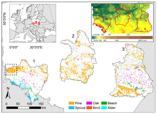
Figure 1.
Location of the regional directorates of state forests used in this study (1—Wroclaw, 2—Lodz, 3—Lublin) and spatial distribution of the tree species masks in MODIS grid (orange—pine, blue—spruce, purple—oak, green—beech). In the upper right-hand corner the directorates’ borders are presented over the elevation map (source of the elevation map: pl.wikipedia.org, accessed on 21 October 2022). The black dashed line indicates the pine-forested area showcased in detail in this study.
Pine is the most widespread and dominant species in the study area [32], well adapted to living in warm and cold temperate zones and in nutrient-poor soils. In Poland, it grows mostly in the lowlands, and often in a form of a planted monoculture. Such pine forests are present especially in the central region. Unlike pine, oak has greater habitat requirements. Its clusters are present in the lowlands and uplands of Wroclaw and Lublin directorates, occupying up to 14% of the forest area in the latter [33]. In turn, beech and spruce are predominant tree species in upland and mountain habitats, occupying mostly the Roztocze upland in Lublin directorate and the foothill, sub-mountain and mountain regions in the south of Wroclaw directorate. The share of spruce in Wroclaw directorate exceeds 23% of the forest area [34].
A detailed tree species classification [35], based on the tailored machine learning Random Forest algorithm, was prepared on the basis of multi-temporal Sentinel-2 data, following the hierarchical approach proposed by Hościło and Lewandowska [36]. In this study, the Sentinel-2 data acquired in 2021 and 2022 were used to classify eight tree species, namely, pine, spruce, larch, fir, oak, birch, beech and alder. The overall accuracy of pine and spruce reached 94–97% and 74–95%, respectively, whereas the overall accuracy of beech and oak reached 87–93% and 76–85%, respectively.
In order to conduct analyses for four chosen tree species, the respective species masks in the MODIS grid were produced on the basis of the result of the Sentinel-2 classification. To this end, MODIS and Sentinel-2 data were both reprojected onto the WGS84 geographic coordinate system. For each MODIS pixel (which is approx. 250 × 250 m) the number of Sentinel-2 pixels (which are approx. 10 × 10 m) located inside this MODIS grid cell was calculated. The MODIS pixel was assigned as occupied by a particular species if at least 90% of the Sentinel-2 pixels were classified as this particular species. The threshold of 90% was used to assure the homogeneity of forest-species pixels. Following these selection criteria, four separate species masks in the MODIS grid were prepared, with their spatial distribution presented in Figure 1, and the number of retained MODIS pixels and covering area presented in Table 1. A relatively large number of pixels forming each mask reduces the level of uncertainty of the research results.

Table 1.
Number of MODIS pixels in each species mask in three directorates (Wroclaw, Lodz and Lublin) and area (km2) they cover.
2.2. MODIS Data—NDVI and EVI
Two vegetation indices (VI)—NDVI and EVI—derived from MODIS onboard Terra and Aqua satellites [37,38] were used. The products MOD13Q1 and MYD13Q1 available at the spatial resolution of 250 m were downloaded for the time period 2002–2022 from http://search.earthdata.nasa.gov. Similarly, as in, e.g., Buras et al. [5], only the pixels indicated as good or marginal quality were selected. Next, as the MO(Y)D13Q1 products are delivered as 16-day composites, in which the adjacent pixels may originate from different days, so, on the basis of the day-of-year layer (which keeps the information about the actual day the pixel originates), each of the previously selected pixels was allocated to the respective month. For each MODIS pixel, only a maximum value in a given month was taken. As in many similar studies, the assumption that low-value observations are either erroneous or have reduced vegetation vigour for the time period under consideration [39] was applied.
Having monthly maximum NDVI (or EVI) values for each pixel and for each month in the period 2002–2022, we produced standardised NDVI (EVI) values, i.e., z-scores, similar to, e.g., Hościło et al. [40]. Because the course of monthly VI values shows a natural annual cycle, the monthly mean NDVI (EVI) values were standardised separately for each month, according to the following formula (Equation (1)):
where is the monthly maximum NDVI value in the m-th month (e.g., in a given January in a given year) and in the i-th pixel; and are the mean and standard deviation values of monthly maximum NDVI values in all m-th months (e.g., in all the January months) and in i-th pixel. Z-scores for the respective EVI values were prepared.
Finally, a spatially averaged 252-element (12 months in each year of the 2002–2022 period) time series of NDVI z-scores (or EVI z-scores) in the respective tree species masks were prepared. They were calculated as area averages of all NDVI z-scores (or EVI z-scores) in the MODIS grid cells within the respective species masks.
2.3. Meteorological Elements
To visualise climatic conditions, monthly values of 2-metre temperature (T, in °C) and precipitation (P, in mm), originating from ERA5-Land reanalysis [41,42], were used. Data were downloaded from the Copernicus Data Store (https://cds.climate.copernicus.eu/) for the same time period of 2002–2022. As ERA5-Land has a resolution of 0.1° × 0.1°, it was resampled to fit the MODIS grid cells using the nearest-neighbour-interpolation method. Then, standardised values of T and P, i.e., z-scores, were produced in the same way as NDVI z-scores (Equation (1)). In the next step, the masking for species was applied. Comparing to the vegetation condition, which may change very dynamically from one pixel to another, meteorological elements are rather slowly changing in space. That is why only one mask, including all four tree species and consisting of 36,815 pixels in total, was applied to T and P. Finally, area averages of all z-scores for T and P in the MODIS grid cells within the all species masks were prepared, resulting in a 252-element time series of z-scores for T and P. These time series represent well the meteorological conditions for all of the four species.
2.4. Methods
In order to identify the trend for changes in the NDVI and EVI z-scores, several research methods were adopted. The slopes of the linear trends of NDVI z-scores (or EVI z-scores) in moving periods were computed for each of the four species. The statistical significance of these slopes was assessed (at the level of significance α = 0.05) and the p-values were presented. The only parameterization required is the length of the moving period, which should be carefully selected to provide useful information—not too generalized, but also not too detailed and therefore difficult to interpret. Simulations with different lengths of the moving period allowed us to select a 60-month (5-year) period, corresponding to 24% of the 21-year data span. This method allows us to indicate periods of a significant positive and negative trend. The period in which the slope-value switches sign (from significant positive to significant negative, or vice versa) can be identified as a period with a change in trend. The middle year of that period can be treated as a trend change point. However, the course of the slope values should be interpreted visually, and with same caution, and the resulting information might be approximate.
The years of a probable occurrence of the changes in trend were additionally identified with the Bayesian Estimator of Abrupt change, Seasonal change and Trend (BEAST). The BEAST method was introduced by Zhao et al. [43], and the detailed description of this method, together with its validation and usage examples, can be found there [43]. In general, it is a generic tool for detecting change point, trend, and seasonality in time series, although in the case of purposedly standardised z-scores, the seasonality is not being detected. The algorithm can run without any initial assumptions, but in this study we introduced a minimum trend segment length of 60 months (5 years), in order to maintain consistency with the previous analyses.
In the next step, the course of z-scores is presented, together with linear trends for the shorter periods detected. The linear trends are given, together with the coefficient of determination R2 and the p-value (in order to assess the statistical significance of the trends). To better illustrate how these trends fit the course of z-scores for the NDVI and EVI, the z-scores were additionally filtered with a running 37-month (ca. 3-year) mean.
The analysis of meteorological elements was prepared in a similar manner to that for VI. The slopes of the linear trends of z-scores for T and P in moving periods were computed, as well as the years of a probable occurrence of the changes in trend (using the BEAST method). The courses of z-scores for T and P are presented, together with linear trends for the shorter periods detected, the R2 and p-value, with additional running 37-month (ca. 3-year) mean.
Finally, for a small area with relatively high coverage of pine forest (indicated in Figure 1), in order to better illustrate the detected periods of greening and browning, we present the spatial distribution of the slopes of the trends in NDVI z-scores, calculated at the pixel level. The slopes were calculated for each of the detected periods separately, and their statistical significance was assessed at the significance level α = 0.05.
3. Results
The main pattern behind the observed course of trends for four main forest-forming tree species is similar, to some extent, and shows an increase for both NDVI and EVI z-scores, but it differs with a close-up look at particular species.
Pine is the only species with a statistically significant downward trend at the beginning of the analysed period, clearly visible in NDVI z-scores, but noticeable also for EVI z-scores (Figure 2 and Figure 3). This downward trend has the steepest slope, of −0.013 for NDVI z-scores (or −0.010 for EVI z-scores) and is statistically significant in the period 2002–2006 (Figure 4 and Figure 5). Many negative, statistically significant slopes of the linear trend in NDVI z-scores, reaching −0.060·month−1, are visible in this period in the pine-forested area in Figure 6a. The slope in running periods turns positive in the 2003–2007 period (Figure 2), suggesting 2005 or 2006 as a moment of change. The year 2006 is also detected as a trend change point, according to the BEAST method results, with a very high probability of occurrence (0.999) (Table 2). In the following 5-year moving periods, the slope of the linear trend in z-scores of both VIs is positive, with bigger (significant) and lower (insignificant) values until the 2013–2017 period, when the slope changes into a negative value. Taking the middle year of this period as a moment when the negative trend starts, it seems that the year 2015 can be assumed as another trend change point. The BEAST method, however, suggests year 2017, with a lower probability of occurrence (0.822), as a secondary trend change point. The increase in pine condition, described by z-scores of both VIs, was significant in years 2006–2015, and amounted to 0.009·month−1 and 0.006·month−1 for z-scores of NDVI and EVI, respectively (Figure 4 and Figure 5). Many positive and significant slopes reaching 0.025·month−1 are also visible in this period in Figure 6b. After 2015, the trend in condition of pines shows no clear direction. The 5-year moving periods from 2014–2018 to 2016–2020 have significant negative slopes, followed by significant positive slopes in the moving periods 2017–2021 onwards (Figure 2 and Figure 3). This suggests that a third trend change point can be identified in 2019. However, the downward trend in the period 2015–2019 is statistically significant only for NDVI z-scores (and insignificant for EVI). The opposite is the case with respect to the upward trend in years 2019–2022, which is significant only for EVI z-scores (Figure 4 and Figure 5).
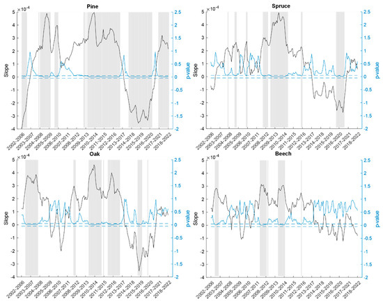
Figure 2.
The slopes (z-score for NDVI·month−1) of the linear trends of monthly NDVI z-scores over four species (pine, spruce, oak and beech) (black lines) and their p-values (blue lines) from 2002 to 2022 in moving 5-year (60-month) periods. The statistical significance level of α = 0.05 is indicated by blue dashed lines. Statistically significant slopes are additionally highlighted with a grey colour.
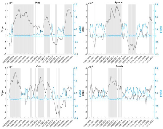
Figure 3.
The slopes (z-score for EVI·month−1) of the linear trends of monthly EVI z-scores over four species (pine, spruce, oak and beech) (black lines) and their p-values (blue lines) from 2002 to 2022 in moving 5-year (60-month) periods. The statistical significance level of α = 0.05 is indicated by blue dashed lines. Statistically significant slopes are additionally highlighted with a grey colour.
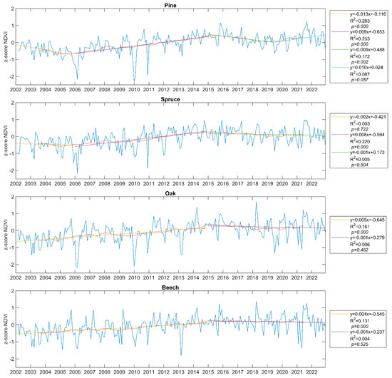
Figure 4.
The course of NDVI z-scores (blue line) for four tree species (pine, spruce, oak and beech) in the period 2002–2022. The graphs also present the running 37-month mean (orange line) and linear trends for the shorter periods (coloured are lines explained next to each graph), together with trend line equations, coefficients of determination R2 and p-values.
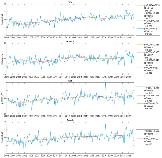
Figure 5.
The course of EVI z-scores (blue line) for four tree species (pine, spruce, oak and beech) in the period 2002–2022. The graphs also present the running 37-month mean (orange line) and linear trends for the shorter periods (coloured lines are explained next to each graph), together with trend line equations, coefficients of determination R2 and p-values.
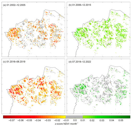
Figure 6.
Slopes of the trends in NDVI z-scores (z-score for NDVI·month−1) in a selected pine-forested area in regional directorate of state forests in Wroclaw (location of this area is presented in Figure 1), in the periods 01.2002–12.2005 (a), 01.2006–12.2015 (b), 01.2016–06.2019 (c) and 07.2019–12.2022 (d). Grey colour indicates insignificant slopes at the significance level of α = 0.05.

Table 2.
Years of a probable change in trend and their probability of occurrence, identified with the BEAST method, for four species (z-scores for NDVI and EVI) and for meteorological elements (z-scores T and P), in the period 2002–2022.
A similar pattern, but not so pronounced, is visible in the course of z-scores for NDVI and EVI for spruce. The decrease in spruce forest condition at the beginning of the analysed period is hardly visible (Figure 2 and Figure 3). According to the BEAST method results, the year of a most probable change in trend is 2010 (Table 2), which is puzzling, because no such change in trend is identified in moving-period trend slopes. It might suggest a possible limitation or imperfection of the BEAST method. Instead, a steady increase in condition of spruces occurred in years 2006–2015, with a slope of the linear trend as steep as 0.008·month−1 and 0.007·month−1 for z-scores for NDVI and EVI, respectively (Figure 4 and Figure 5). In the following years, although the moving-period trend slopes are alternately negative and positive, with many significant moments (Figure 2 and Figure 3), the trend in z-scores of both VIs is rather indifferent (Figure 4 and Figure 5).
Broadleaved species present an even more stable pattern in the course of z-scores for NDVI and EVI. Positive (and significant in some parts) trends for oak and beech, with some minor negative exceptions, are visible from the beginning (2002) until the 2013–2017 moving period (Figure 2 and Figure 3). Again, the middle year of this period—2015—can be assumed as a trend change point. Hence, in the period 2002–2015, a steady increase (greening) in the condition of oak can be identified, with the slope of the linear trend in z-scores for NDVI and EVI amounting to 0.005·month−1 (Figure 4 and Figure 5). Beech has a similar value of 0.005·month−1 and 0.004·month−1 for z-scores for NDVI and EVI, respectively (Figure 4 and Figure 5).
After 2015, the pattern for oak and beech is slightly different. Concerning oak, the moving-period trend slopes are negative for some time, with some statistically significant decreasing trend slopes (2014–2018 and 2015–2019), but they turn positive (and insignificant) at the end of the period considered (from 2017–2021 onwards). It might suggest a secondary trend change point in 2019, similar to the one detected for pines. However, the trends prepared for such sub-periods (2015 to 2019 and 2019 to 2022) for EVI z-scores, although having slopes of −0.005·month−1 and 0.008·month−1, respectively, are not statistically significant (Figure 5). Insignificant also, is the trend slope for whole 2015–2022 period calculated for NDVI z-scores (Figure 4). In turn, beech shows no clear trend whatsoever. In the period 2015–2022, the trend slope of −0.001·month−1 for NDVI z-scores and 0.003·month−1 for EVI z-scores is insignificant (Figure 4 and Figure 5). The BEAST algorithm indicates, additionally, the year 2011 as a possible trend change point in NDVI z-scores for oak and beech (Table 2). However, the possibility of occurrence of these change points is not very high, and they do not seem to reflect the actual changes in the course of NDVI z-scores.
T is generally increasing in the whole study period, with the significant trend of 0.003 z-score·month−1. Yet, similarly to the VI z-scores, we can determine the shorter periods of an upward and downward trend. The slope of the linear trend in z-scores for T is positive in the moving periods from 2002–2006 until 2005–2009, when the slope changes into a negative value. The middle year of this period—2007—might be assumed as a first trend change point (Figure 7a). However, T shows an indifferent trend at the beginning of the analysed period, in years 2002–2007 (Figure 8a). The next point of changing trend might be considered in the middle of the 2007–2012 period, when the slope turns positive again, i.e., around the year 2010–2011 (Figure 7a). Hence, the decrease in T is significant in the years 2007–2011, and amounts to −0.021·month−1 (Figure 8a). After 2011, in the following moving periods the slope of the linear trend in T z-scores is positive until ca. 2019, when it changes into negative values (a negative value in the 2013–2017 period is very small, and can be disregarded). The upward trend in the years 2011–2019 has the slope of 0.009, and is statistically significant. On the other hand, the year 2013—indicated by the BEAST method—has a rather low probability of occurrence (0.639), and does not seem to reflect the actual changes in the course of T z-scores.
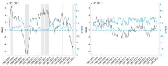
Figure 7.
The slopes (z-score·month−1) of the linear trends of monthly z-scores for T (a) and P (b) and their p-values (blue lines) from 2002 to 2022 in moving 5-year (60-month) periods. The statistical significance level of α = 0.05 is indicated by blue dashed lines. Statistically significant slopes are additionally highlighted with a grey colour.
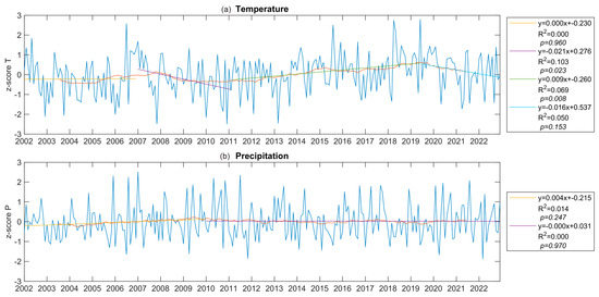
Figure 8.
The course of z-scores (blue lines) for T (a) and P (b) in the period 2002–2022. The graphs also present the running 37-month mean (orange line) and linear trends for the shorter periods (coloured lines are explained next to each graph), together with trend line equations, coefficients of determination R2 and p-values.
When it comes to z-scores for P, results show an indifferent trend for the whole time period (slope 0.001, p-value 0.451). Although the slope of the linear trend in 5-year running periods turns positive and negative several times, none of these slopes are statistically significant (Figure 7b), so it is hard to determine any trend changing points. The BEAST algorithm shows the year 2009 (with very low probability of occurrence), but shorter periods established in that way—2002–2009 and 2010–2022—also have indifferent and insignificant trends (Figure 8b).
4. Discussion
This study documents the general greening of forest species in the period 2002–2022. The predominant species, pine, has a generally increasing trend of 0.004 for NDVI z-score per month, which calculates back to an approximately 0.02 NDVI increase in the whole 21-year period. A similar increase of NDVI over 20 years (0.009 to 0.030) was indicated by Kulesza and Hościło [22] for the mask of all the forest and for the area of the whole of Poland. Since pine forest covers 58% of the forest area in Poland [32], the results obtained for pine can be representative for all the forest.
In general, a pattern of three major contrasting trends in the course of VI z-scores of was detected. The main trend change points might be considered ca. 2006 and ca. 2015. The decreasing trend of z-scores for NDVI and EVI from the beginning of the analysed period until 2006 is mostly visible for pine. Such a decreasing tendency of vegetation productivity, also called browning, is in line with many research results worldwide [15,25,28,29], although individual researchers indicate the trend change point in slightly different years: 2004 [15], 2006 [28,44] or 2008 [25]. The results of Piao et al. [28] are of special interest, because they analysed only the temperate and boreal Eurasia forests, and found that the growing season NDVI has decreased from 1997 to 2006. The reason for this may be related to the remarkable decrease in summer precipitation [28]. Indeed, a severe drought occurred in Europe in 2003, but its impact on vegetation in our study area was not so intense [45]—z-scores for T do not show very substantial anomalies in 2003. Instead, a peak in T in July 2006, combined with a negative z-score for P in the same month, might have facilitated browning of coniferous species.
This decreasing tendency was absent in the course of z-scores for NDVI and EVI for broadleaved species, i.e., oak and beech. These two tree species demonstrate rather steady and slow growth in vegetation condition until 2015. Also, the coniferous tree species—pine and spruce—have steep positive slopes for the linear trends in the period from 2006 to 2015. A rapid greening trend was also detected in many regions worldwide, including central Asia in the years 2008–2022 [25], and north Africa and eastern Siberia in 2005–2012 [15], although central Europe was in the area of mostly insignificant trends (2005–2012) [15]. Yang et al. [44] noticed that greening trends of northwestern China widely expanded after 2006, due to droughts that happened before and sudden intensity in precipitation, starting from 2006. Many researchers attribute the recent growth of vegetation to contemporary climate changes, pointing out that increase in the atmospheric CO2 concentration boosts vegetation productivity and might be one of the key drivers of the NDVI positive trends [19,26,27].
Z-scores for T present a negative trend from 2007 to 2011, then turn into a positive one. The biggest positive peaks in the course of T z-scores are in 2006, then in 2015, 2018 and 2019. Indeed, in 2015 an intense and spatially extended drought affected Europe, including, especially, its eastern part [46]. Subsequent severe droughts occurred in Europe in 2018 [5,47,48], 2019 [48,49] and 2022 [50,51]. Such unprecedented occurrence of consecutive summer droughts led to the inhibition of the existing growth shown in the VIs. All four tree species show a reduction in growth rate (insignificant trends with slopes close to zero), and some (pine) even show a negative trend for NDVI z-scores in the period 2016–2019. However, starting from 2019 or 2020 there is—again—a positive tendency in pine’s course of z-scores for NDVI and EVI. Combining z-scores for NDVI and EVI with z-scores for T and P, one can see a moderate positive correlation between VI and T (Figure 9a,b). However, in many cases of very high temperature (z-score T > 2), z-scores for NDVI and EVI are below or close to 0. This may suggest that droughts, especially these large-scale and persistent ones, are responsible for the decline in vegetation [29]. Some researchers suggest that vegetation browning has progressively increased, globally, against a background of climate change [52]. Others claim that compound droughts only slow down the greening of the Earth [53] and that global greening continues, despite increased drought stress since 2000 [54].
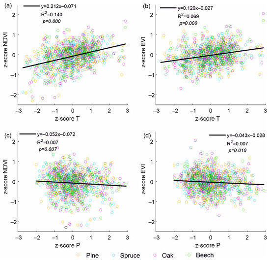
Figure 9.
Relationship between z-scores for T (a,b) and P (c,d) and z-scores for NDVI (a,c) and EVI (b,d) over four species (pine, spruce, oak and beech) from 2002 to 2022. Each graph consist of 1008 points (252 points for each species), and also presents linear regression (black line), together with regression equation, coefficient of determination R2 and p-value.
Forest resilience to droughts varies across biomes, forest types, forest stands and species [55]. Climate change may also contribute significantly to shift in species composition [56], favouring the deciduous species over the coniferous ones [57]. In general, the latter are more sensitive to drought-related disturbances than deciduous species [55,58]. Indeed, the deciduous species analysed in this study (oak and beech) did not show the decrease in vegetation condition, either at the beginning or at the end of the period considered. However, most analyses of spectral indices of vegetation condition that report browning are conducted for the whole world or a whole continent, so they concern only vegetation in general or a simple division into e.g., forest and grassland vegetation. These browning trends might thus be affected by one or few species only, as, e.g., pine, which exceeds 20% of the European productive forest area [59]. Therefore, such detailed analysis of individual species’ greening, browning and trend change points is crucial and should be performed in the future for more species and for increasingly longer time series.
The analysis performed in this study has also some limitations, the first of which is the underlying tree species classification. It was prepared on the basis of Sentinel-2 data acquired in 2021 and 2022, so it only applies to the trees still growing in the end of the study period. However, some trees might have died and been removed within sanitation felling before these years, and therefore the overall greening reported in this study might be slightly overestimated. Moreover, the VI time series analysed in this study are averaged from 1730 (for beech) up to 28,615 (for pine) pixels. It means that local problems that affect individual tree clusters (e.g., browning caused by biotic factors, like bark beetle) disappear into an overall greening.
The method of detecting slopes in moving periods is not resistant to outliers that disturb the course of z-scores, such as, e.g., very-high-temperature outliers that accompany a drought. However, the occurrence of severe droughts has been the main factor ruling greening and browning in recent years, so in our opinion it is not necessary to make this method more robust to outliers.
Finally, attention should be given to the interpretation of the spectral indices’ values. It should be remembered that in remote sensing of forests, the coming NDVI signal reflects not only the tree’s vigour, but also the “noise” from the understorey or soil as well, as it is sensitive to atmospheric influence [6]. Another limitation of the NDVI index is the saturation effect, i.e., insensitivity to changes after a certain level of biomass is reached. For deciduous forests, this level is above 100 Mg·ha−1 [60]. Furthermore, the changes in the course of forest condition can come not only from the drought-related or—more precisely—temperature-related factors. There are other factors that should be kept in mind, such as forest/species site condition, age structure of forests/species or forest management practices, which may drive greening/browning trends, or constitute an important component. Even more reasons, both non-climatic and anthropogenic, can rule browning, e.g., insect or pathogen outbreaks. In the context of future research, it will be very important to recognise in detail for each species where the individual change points and reduced or increased values of the VI come from.
5. Conclusions
This paper presents the course of z-scores for NDVI and EVI for four main forest-forming tree species in the temperate zone: pine, spruce, oak and beech, in the period 2002–2022. We identified the probable trend change points and periods of quasi-stable greening and browning in time series of spectral indices of vegetation condition. To this end, several research approaches, including calculating the linear trends in the moving periods and the BEAST algorithm, were adapted. Using different research methods as well as different spectral indices leads to objectifying the results obtained.
A pattern of browning–greening–constant was detected for coniferous species, mostly pine. In turn, for broadleaved species, namely oak and beech, a pattern of greening–constant was identified, without the initial phase of browning. The main trend change points seem to be ca. 2006 and ca. 2015 for coniferous species, and solely around 2015 for deciduous ones.
Our analysis, extending up to the year 2022, shows the greening and browning trends occurring in the recent years that are not covered by many papers, so far. Additionally, it gives some insight into individual species’ vulnerability to drought-related disturbances. In the near future, similar analyses should be performed for more forest-dominating species and for increasingly longer periods of time.
Author Contributions
K.K.: Conceptualization, methodology, formal analysis, investigation, data curation, writing—original draft, writing—review and editing, visualization. A.H.: Conceptualization, writing—review and editing, supervision, project administration, funding acquisition. All authors have read and agreed to the published version of the manuscript.
Funding
This work was supported by the National Science Centre in Poland [grant number 2021/41/B/ST10/04113].
Data Availability Statement
The data that support the findings of this study were derived from the following resource available in the public domain: https://lpdaac.usgs.gov/products/, https://cds.climate.copernicus.eu/.
Conflicts of Interest
The authors declare that they have no conflicts of interest.
References
- FAO; UNEP. The State of the World’s Forests 2020. In Forests, Biodiversity and People; FAO and UNEP: Rome, Italy, 2020. [Google Scholar]
- Pan, Y.; Birdsey, R.A.; Phillips, O.L.; Jackson, R.B. The Structure, Distribution, and Biomass of the World’s Forests. Annu. Rev. Ecol. Evol. Syst. 2013, 44, 593–622. [Google Scholar] [CrossRef]
- Forest Europe. State of Europe’s Forests 2020; Ministerial Conference on the Protection of Forests in Europe—FOREST EUROPE, Liaison Unit Bratislava: Bonn, Germany, 2020. [Google Scholar]
- Myneni, R.B.; Keeling, C.D.; Tucker, C.J.; Asrar, G.; Nemani, R.R. Increased plant growth in the northern high latitudes from 1981 to 1991. Nature 1997, 386, 698–702. [Google Scholar] [CrossRef]
- Buras, A.; Rammig, A.; Zang, C.S. Quantifying impacts of the 2018 drought on European ecosystems in comparison to 2003. Biogeosciences 2020, 17, 1655–1672. [Google Scholar] [CrossRef]
- Huang, S.; Tang, L.; Hupy, J.P.; Wang, Y.; Shao, G. A commentary review on the use of Normalized Difference Vegetation Index (NDVI) in the era of popular remote sensing. J. For. Res. 2021, 32, 1–6. [Google Scholar] [CrossRef]
- Soubry, I.; Doan, T.; Chu, T.; Guo, X. A Systematic Review on the Integration of Remote Sensing and GIS to Forest and Grassland Ecosystem Health Attributes, Indicators, and Measures. Remote Sens. 2021, 13, 3262. [Google Scholar] [CrossRef]
- Gomez, D.F.; Ritger, H.M.W.; Pearce, C.; Eickwort, J.; Hulcr, J. Ability of Remote Sensing Systems to Detect Bark Beetle Spots in the Southeastern US. Forests 2020, 11, 1167. [Google Scholar] [CrossRef]
- Brun, P.; Psomas, A.; Ginzler, C.; Thuiller, W.; Zappa, M.; Zimmermann, N.E. Large-scale early-wilting response of Central European forests to the 2018 extreme drought. Glob. Chang. Biol. 2020, 26, 7021–7035. [Google Scholar] [CrossRef] [PubMed]
- Galvao, L.S.; dos Santos, J.R.; Roberts, D.A.; Breunig, F.M.; Toomey, M.; de Moura, Y.M. On intra-annual EVI variability in the dry season of tropical forest: A case study with MODIS and hyperspectral data. Remote Sens. Environ. 2011, 115, 2350–2359. [Google Scholar] [CrossRef]
- Moreira, A.; Fontana, D.C.; Kuplich, T.M. Wavelet approach applied to EVI/MODIS time series and meteorological data. ISPRS J. Photogramm. Remote Sens. 2019, 147, 335–344. [Google Scholar] [CrossRef]
- Zoungrana, B.J.-B.; Conrad, C.; Amekudzi, L.K.; Thiel, M.; Da, E.D. Land Use/Cover Response to Rainfall Variability: A Comparing Analysis between NDVI and EVI in the Southwest of Burkina Faso. Climate 2015, 3, 63–77. [Google Scholar] [CrossRef]
- Huete, A.; Didan, K.; Miura, T.; Rodriguez, E.P.; Gao, X.; Ferreira, L.G. Overview of the radiometric and biophysical performance of the MODIS vegetation indices. Remote Sens. Environ. 2002, 83, 195–213. [Google Scholar] [CrossRef]
- Didan, K.; Munoz, A.B. MODIS Vegetation Index User’s Guide (MOD13 Series); Vegetation Index and Phenology Lab, The University of Arizona: Tucson, AZ, USA, 2019. [Google Scholar]
- Liu, Y.; Li, Y.; Li, S.; Motesharrei, S. Spatial and Temporal Patterns of Global NDVI Trends: Correlations with Climate and Human Factors. Remote Sens. 2015, 7, 13233–13250. [Google Scholar] [CrossRef]
- Guo, M.; Li, J.; He, H.; Xu, J.; Jin, Y. Detecting Global Vegetation Changes Using Mann-Kendal (MK) Trend Test for 1982–2015 Time Period. Chin. Geogr. Sci. 2018, 28, 907–919. [Google Scholar] [CrossRef]
- Yang, Y.; Wang, S.; Bai, X.; Tan, Q.; Li, Q.; Wu, L.; Tian, S.; Hu, Z.; Li, C.; Deng, Y. Factors Affecting Long-Term Trends in Global NDVI. Forests 2019, 10, 372. [Google Scholar] [CrossRef]
- Ding, Z.; Peng, J.; Qiu, S.; Zhao, Y. Nearly Half of Global Vegetated Area Experienced Inconsistent Vegetation Growth in Terms of Greenness, Cover, and Productivity. Earth’s Future 2020, 8, e2020EF001618. [Google Scholar] [CrossRef]
- de Jong, R.; Verbesselt, J.; Schaepman, M.E.; de Bruin, S. Trend changes in global greening and browning: Contribution of short-term trends to longer-term change. Glob. Chang. Biol. 2012, 18, 642–655. [Google Scholar] [CrossRef]
- Prăvălie, R.; Sîrodoev, I.; Nita, I.-A.; Patriche, C.; Dumitraşcu, M.; Roşca, B.; Tişcovschi, A.; Bandoc, G.; Săvulescu, I.; Mănoiu, V.; et al. NDVI-based ecological dynamics of forest vegetation and its relationship to climate change in Romania during 1987–2018. Ecol. Indic. 2022, 136, 108629. [Google Scholar] [CrossRef]
- Kempf, M. Enhanced trends in spectral greening and climate anomalies across Europe. Environ. Monit. Assess. 2023, 195, 260. [Google Scholar] [CrossRef]
- Kulesza, K.; Hościło, A. Influence of climatic conditions on Normalized Difference Vegetation Index variability in forest in Poland (2002–2021). Meteorol. Appl. 2023, 30, e2156. [Google Scholar] [CrossRef]
- Berner, L.T.; Goetz, S.J. Satellite observations document trends consistent with a boreal forest biome shift. Glob. Chang. Biol. 2022, 28, 3275–3292. [Google Scholar] [CrossRef]
- Cortés, J.; Mahecha, M.D.; Reichstein, M.; Myneni, R.B.; Chen, C.; Brenning, A. Where Are Global Vegetation Greening and Browning Trends Significant? Geophys. Res. Lett. 2021, 48, e2020GL091496. [Google Scholar] [CrossRef]
- Su, Y.; Chen, S.; Li, X.; Ma, S.; Xie, T.; Wang, J.; Yan, D.; Chen, J.; Feng, M.; Chen, F. Changes in vegetation greenness and its response to precipitation seasonality in Central Asia from 1982 to 2022. Environ. Res. Lett. 2023, 18, 104002. [Google Scholar] [CrossRef]
- Nemani, R.R.; Keeling, C.D.; Hashimoto, H.; Jolly, W.M.; Piper, S.C.; Tucker, C.J.; Myneni, R.B.; Running, S.W. Climate-Driven Increases in Global Terrestrial Net Primary Production from 1982 to 1999. Science 2003, 300, 1560–1563. [Google Scholar] [CrossRef] [PubMed]
- Piao, S.; Friedlingstein, P.; Ciais, P.; Zhou, L.; Chen, A. Effect of climate and CO2 changes on the greening of the Northern Hemisphere over the past two decades. Geophys. Res. Lett. 2006, 33, L23402. [Google Scholar] [CrossRef]
- Piao, S.; Wang, X.; Ciais, P.; Zhu, B.; Wang, T.; Liu, J. Changes in satellite-derived vegetation growth trend in temperate and boreal Eurasia from 1982 to 2006. Glob. Chang. Biol. 2011, 17, 3228–3239. [Google Scholar] [CrossRef]
- Zhao, M.; Running, S.W. Drought-Induced Reduction in Global Terrestrial Net Primary Production from 2000 Through 2009. Science 2010, 329, 940–943. [Google Scholar] [CrossRef] [PubMed]
- Matas-Granados, L.; Pizarro, M.; Cayuela, L.; Domingo, D.; Gómez, D.; García, M.B. Long-term monitoring of NDVI changes by remote sensing to assess the vulnerability of threatened plants. Biol. Conserv. 2022, 265, 109428. [Google Scholar] [CrossRef]
- Tomczyk, A.M.; Bednorz, E. Atlas klimatu Polski (1991–2020); Bogucki Wydawnictwo Naukowe: Poznan, Poland, 2022. [Google Scholar]
- Zajączkowski, G.; Jabłoński, M.; Jabłoński, T.; Sikora, K.; Kowalska, A.; Małachowska, J.; Piwnicki, J. (Eds.) Raport o Stanie Lasów w Polsce 2021; Centrum Informacyjne Lasów Państwowych: Warsaw, Poland, 2022. [Google Scholar]
- RDLP Lublin. Lasy Regionu. Available online: https://www.lublin.lasy.gov.pl/lasy-regionu (accessed on 14 December 2023).
- Zięba, M. Lasy Regionu. Available online: https://www.wroclaw.lasy.gov.pl/lasy-regionu (accessed on 14 December 2023).
- Hościło, A.; Rynkiewicz, A.; Wasik, A.; Stosio, D. Klasyfikacja Głównych Gatunków Drzew na Podstawie Danych Sentinel-2; Instytut Geodezji i Kartografii: Warsaw, Poland, 2023. [Google Scholar]
- Hościło, A.; Lewandowska, A. Mapping Forest Type and Tree Species on a Regional Scale Using Multi-Temporal Sentinel-2 Data. Remote Sens. 2019, 11, 929. [Google Scholar] [CrossRef]
- Didan, K. MODIS/Aqua Vegetation Indices 16-Day L3 Global 250m SIN Grid V061 [Data Set]; NASA EOSDIS Land Processes DAAC, 2021. Available online: https://lpdaac.usgs.gov/products/myd13q1v061/ (accessed on 4 December 2022).
- Didan, K. MODIS/Terra Vegetation Indices 16-Day L3 Global 250m SIN Grid V061 [Data Set]; NASA EOSDIS Land Processes DAAC, 2021. Available online: https://lpdaac.usgs.gov/products/mod13q1v061/ (accessed on 4 December 2022).
- Holben, B.N. Characteristics of maximum-value composite images from temporal AVHRR data. Int. J. Remote Sens. 1986, 7, 1417–1434. [Google Scholar] [CrossRef]
- Hościło, A.; Balzter, H.; Bartholomé, E.; Boschetti, M.; Brivio, P.A.; Brink, A.; Clerici, M.; Pekel, J.F. A conceptual model for assessing rainfall and vegetation trends in sub-Saharan Africa from satellite data. Int. J. Climatol. 2015, 35, 3582–3592. [Google Scholar] [CrossRef]
- Muñoz-Sabater, J. ERA5-Land Hourly Data from 1981 to Present. Copernicus Climate Change Service (C3S) Climate Data Store (CDS). 2019. 4.11.2022. Available online: https://cds.climate.copernicus.eu/cdsapp#!/dataset/10.24381/cds.e2161bac?tab=overview (accessed on 4 November 2022).
- Muñoz-Sabater, J.; Dutra, E.; Agustí-Panareda, A.; Albergel, C.; Arduini, G.; Balsamo, G.; Boussetta, S.; Choulga, M.; Harrigan, S.; Hersbach, H.; et al. ERA5-Land: A state-of-the-art global reanalysis dataset for land applications. Earth Syst. Sci. Data 2021, 13, 4349–4383. [Google Scholar] [CrossRef]
- Zhao, K.; Wulder, M.A.; Hu, T.; Bright, R.; Wu, Q.; Qin, H.; Li, Y.; Toman, E.; Mallick, B.; Zhang, X.; et al. Detecting change-point, trend, and seasonality in satellite time series data to track abrupt changes and nonlinear dynamics: A Bayesian ensemble algorithm. Remote Sens. Environ. 2019, 232, 111181. [Google Scholar] [CrossRef]
- Yang, L.Q.; Guan, Q.Y.; Lin, J.K.; Tian, J.; Tan, Z.; Li, H.C. Evolution of NDVI secular trends and responses to climate change: A perspective from nonlinearity and nonstationarity characteristics. Remote Sens. Environ. 2021, 254, 112247. [Google Scholar] [CrossRef]
- Somorowska, U. Amplified signals of soil moisture and evaporative stresses across Poland in the twenty-first century. Sci. Total Environ. 2022, 812, 151465. [Google Scholar] [CrossRef] [PubMed]
- Ionita, M.; Tallaksen, L.M.; Kingston, D.G.; Stagge, J.H.; Laaha, G.; Van Lanen, H.A.J.; Scholz, P.; Chelcea, S.M.; Haslinger, K. The European 2015 drought from a climatological perspective. Hydrol. Earth Syst. Sci. 2017, 21, 1397–1419. [Google Scholar] [CrossRef]
- Schuldt, B.; Buras, A.; Arend, M.; Vitasse, Y.; Beierkuhnlein, C.; Damm, A.; Gharun, M.; Grams, T.E.E.; Hauck, M.; Hajek, P.; et al. A first assessment of the impact of the extreme 2018 summer drought on Central European forests. Basic Appl. Ecol. 2020, 45, 86–103. [Google Scholar] [CrossRef]
- Boergens, E.; Güntner, A.; Dobslaw, H.; Dahle, C. Quantifying the Central European Droughts in 2018 and 2019 With GRACE Follow-On. Geophys. Res. Lett. 2020, 47, e2020GL087285. [Google Scholar] [CrossRef]
- Hari, V.; Rakovec, O.; Markonis, Y.; Hanel, M.; Kumar, R. Increased future occurrences of the exceptional 2018–2019 Central European drought under global warming. Sci. Rep. 2020, 10, 12207. [Google Scholar] [CrossRef] [PubMed]
- Buras, A.; Meyer, B.; Rammig, A. Record reduction in European forest canopy greenness during the 2022 drought. In Proceedings of the EGU General Assembly 2023, Vienna, Austria, 24–28 April 2023. [Google Scholar]
- Wang, Y.; Wang, Y.; Zhu, X.; Rammig, A.; Buras, A. Quantifying Tree-species Specific Responses to the Extreme 2022 Drought in Germany. In Proceedings of the EGU General Assembly 2023, Vienna, Austria, 24–28 April 2023. [Google Scholar]
- Liu, Q.; Peng, C.; Schneider, R.; Cyr, D.; Liu, Z.; Zhou, X.; Du, M.; Li, P.; Jiang, Z.; McDowell, N.G.; et al. Vegetation browning: Global drivers, impacts, and feedbacks. Trends Plant Sci. 2023, 28, 1014–1032. [Google Scholar] [CrossRef]
- Liu, X.F.; Sun, G.P.; Fu, Z.; Ciais, P.; Feng, X.M.; Li, J.; Fu, B.J. Compound droughts slow down the greening of the Earth. Glob. Chang. Biol. 2023, 29, 3072–3084. [Google Scholar] [CrossRef]
- Chen, X.; Chen, T.; He, B.; Liu, S.; Zhou, S.; Shi, T. The global greening continues despite increased drought stress since 2000. Glob. Ecol. Conserv. 2024, 49, e02791. [Google Scholar] [CrossRef]
- Gazol, A.; Camarero, J.J.; Vicente-Serrano, S.M.; Sánchez-Salguero, R.; Gutiérrez, E.; de Luis, M.; Sangüesa-Barreda, G.; Novak, K.; Rozas, V.; Tíscar, P.A.; et al. Forest resilience to drought varies across biomes. Glob. Chang. Biol. 2018, 24, 2143–2158. [Google Scholar] [CrossRef]
- Andivia, E.; Ruiz-Benito, P.; Díaz-Martínez, P.; Carro-Martínez, N.; Zavala, M.A.; Madrigal-González, J. Inter-specific tolerance to recurrent droughts of pine species revealed in saplings rather than adult trees. For. Ecol. Manag. 2020, 459, 117848. [Google Scholar] [CrossRef]
- Rigling, A.; Bigler, C.; Eilmann, B.; Feldmeyer-Christe, E.; Gimmi, U.; Ginzler, C.; Graf, U.; Mayer, P.; Vacchiano, G.; Weber, P.; et al. Driving factors of a vegetation shift from Scots pine to pubescent oak in dry Alpine forests. Glob. Chang. Biol. 2013, 19, 229–240. [Google Scholar] [CrossRef]
- Anderegg, L.D.L.; Anderegg, W.R.L.; Berry, J.A. Not all droughts are created equal: Translating meteorological drought into woody plant mortality. Tree Physiol. 2013, 33, 672–683. [Google Scholar] [CrossRef]
- Houston Durrant, T.; de Rigo, D.; Caudullo, G. Pinus sylvestris in Europe: Distribution, habitat, usage and threats. In European Atlas of Forest Tree Species; San-Miguel-Ayanz, J., de Rigo, D., Caudullo, G., Houston Durrant, T., Mauri, A., Eds.; Publication Office of the European Union: Luxembourg, 2016; p. e016b094+. [Google Scholar]
- Van Der Meer, F.; Bakker, W.; Scholte, K.; Skidmore, A.; De Jong, S.; Clevers, J.; Addink, E.; Epema, G. Spatial scale variations in vegetation indices and above-ground biomass estimates: Implications for MERIS. Int. J. Remote Sens. 2001, 22, 3381–3396. [Google Scholar] [CrossRef]
Disclaimer/Publisher’s Note: The statements, opinions and data contained in all publications are solely those of the individual author(s) and contributor(s) and not of MDPI and/or the editor(s). MDPI and/or the editor(s) disclaim responsibility for any injury to people or property resulting from any ideas, methods, instructions or products referred to in the content. |
© 2024 by the authors. Licensee MDPI, Basel, Switzerland. This article is an open access article distributed under the terms and conditions of the Creative Commons Attribution (CC BY) license (https://creativecommons.org/licenses/by/4.0/).