Abstract
Accurate detection of drought stress in plants is essential for water use efficiency and agricultural output. Hyperspectral imaging (HSI) provides a non-invasive method in plant phenotyping, allowing the long-term monitoring of plant health due to sensitivity to subtle changes in leaf constituents. The broad spectral range of HSI enables the development of different vegetation indices (VIs) to analyze plant trait responses to multiple stresses, such as the combination of nutrient and drought stresses. However, known VIs may underperform when subjected to multiple stresses. This study presents new VIs in tandem with machine learning models to identify drought stress in wheat plants under varying nitrogen (N) levels. A pot wheat experiment was set up in the glasshouse with four treatments: well-watered high-N (WWHN), well-watered low-N (WWLN), drought-stress high-N (DSHN) and drought-stress low-N (DSLN). In addition to ensuring that plants were watered according to the experiment design, photosynthetic rate (Pn) and stomatal conductance (gs) (which are used to assess plant drought stress) were taken regularly, serving as the ground truth data for this study. The proposed VIs, together with known VIs, were used to train three classification models: support vector machines (SVM), random forest (RF), and deep neural networks (DNN) to classify plants based on their drought status. The proposed VIs achieved more than 0.94 accuracy across all models, and their performance further increased when combined with known VIs. The combined VIs were used to train three regression models to predict the stomatal conductance and photosynthetic rates of plants. The random forest regression model performed best, suggesting that it could be used as a stand-alone tool to forecast gs and Pn and track drought stress in wheat. This study shows that combining hyperspectral data with machine learning can effectively monitor and predict drought stress in crops, especially in varying nitrogen conditions.
1. Introduction
Despite advancements in agronomic management and breeding procedures, crop productivity remains susceptible to abiotic stresses such as drought. During drought stress, plants close their stomata to conserve water, decreasing the absorption of carbon dioxide required for photosynthesis [1]. Furthermore, drought stress can affect nutrient absorption and cause nutrient imbalances, impacting plant metabolic processes. Hence, developing tools to detect plant drought stress is essential for prompt intervention and management to minimize crop losses.
Conventionally, agronomists and breeders evaluate drought stress by visual grading, for example using the stay-green morphological features of plants [2]. However, this method is subjective and prone to errors since stresses like iron and nitrogen deficiency could exhibit similar stress symptoms. Multiple approaches, including gas exchange measurements—stomatal conductance (gs) and photosynthetic rate (Pn) [3], soil moisture monitoring [4], leaf temperature measurement [5], and water potential assessment [6], have been deployed to detect drought stress in plants. While these methods provide detailed and precise information, they have low throughput and may have limited applicability to field conditions. Furthermore, some of these methods are invasive, limited to real-time monitoring, and subject to the spatial variability of field crops.
With advancements in computer vision, remote sensing data derived from different sensors, such as thermal, visible, and hyperspectral imaging (HSI), can effectively detect and monitor the temporal and spatial impact of drought conditions [7,8]. Recently, there has been a surge of interest in HSI applications for abiotic stress assessment, especially nutrient and drought stress analysis. Drought stress leads to subtle modifications in the chemical, physiological, and structural components of plants, which can be detected within the short-wave infrared region (1300–1500 nm) of the spectrum [9]. With prolonged drought stress, there are changes in leaf pigments, which can also be measured through the spectral variations in the visible region [10]. The complex dynamics of drought stress initiation and progression suggest that a single spectral band or VIs could be insufficient in detecting and monitoring drought stress over time.
One standard method for analyzing HSI data in plant phenotyping is to extract vegetation indices (VIs), which are mathematical combinations of spectral reflectance characteristics of vegetation at different wavelengths [11]. VIs have the benefit of reducing the effect of scale factors, including lighting conditions and slope effects [12]. VIs such as the renormalized difference vegetation index (RDVI), normalized photochemical reflectance index (PRInorm), photochemical reflectance index (PRI570), normalized difference vegetation index (NDVI), water index (WI), and normalized water index (NWI) have been used to detect drought stress and monitor its progression. Ihuoma and Madramootoo [13] presented a review of different VIs for monitoring plant drought stress for irrigation management.
To develop VIs for stress monitoring, spectral averaging, which calculates the average spectrum over the pixel domain, is performed after pre-processing. After spectral averaging, the resulting data are still huge and multicollinear. The high-dimensional features can cause algorithmic instability, which can affect the accuracy of data analysis [14]. Moreover, from the hundreds of wavelengths scanned, only a small subset may be associated with the desired trait; the remainder is usually redundant or irrelevant, which may increase the computational processing and overfitting. The high-dimensional data may also be susceptible to noise and non-uniformity, which may affect the interpretation and accuracy of the analysis. This may be mitigated by employing dimensionality reduction techniques, either feature extraction or selection. In feature extraction, the data are transformed from a high to a low-dimensional space. In contrast, a subset of relevant features from the original hyperspectral datasets is selected for feature selection, discarding redundant or irrelevant ones. Linear discriminant analysis (LDA) and principal component analysis (PCA) are examples of feature extraction methods. Filter (e.g., ReliefF and correlation-based feature selection [15]), wrapper (sequential feature selection, recursive feature elimination [16,17]), and embedding techniques (e.g., random forest and LASSO [18]) are examples of feature selection methods. Remeseiro and Bolon-Canedo [19] documented the detailed operation of different feature selection methods for HSI analysis. Determining a standard method to select spectral features in HSI analysis is challenging despite the availability of several feature selection methods [20]. Each feature selection strategy has its benefits and setbacks. Ensemble learning methods that combine the predictions of multiple selection methods to improve the overall accuracy and robustness of models are often employed to minimize the effect of using a single feature selection model.
Machine learning (ML) models have been widely used for hyperspectral data analysis because they handle complex data patterns and relationships. ML methods such as support vector machines (SVM) and random forest (RF), among others, have been used to evaluate the predictive power of multiple spectral indices for plant drought [7] and nutrient stress [21] analysis. Pairing whole spectra, extracted features, or selected features with different ML methods can improve the accuracy of plant drought stress classification. VIs are usually developed for specific stresses and may fail in plants with multiple stresses.
The relationship between drought stress and plant N content is complex and has a substantial effect on plant growth and development. Nitrogen contributes to the production of stress-related compounds such as osmoprotectants and secondary metabolites, which enable plants to cope with drought stresses [22]. However, high N levels promote vegetative growth, which subsequently leads to increased water requirements of the plants. This can exacerbate the effects of drought stress in plants [23]. Furthermore, low N levels lead to a decrease in photosynthetic efficiency, which is already compromised during drought, leading to huge reductions in plant photosynthetic rates [24]. Since N is a critical component of proteins affecting plant stomatal behavior and water-use efficiency, understanding the dynamics of plant spectral characteristics in response to drought stress under different N contents is essential. From previous studies [25,26], adequate N content promotes the growth and yield of plants. However, excess N levels may increase plant water demand, potentially worsening drought stress. There is little knowledge on the non-invasive assessment of excess or inadequate N levels on plants with variable water content.
This study aims to understand plant canopy spectral interactions under different N and water levels. First, we examined the effectiveness of using various known VIs to assess plant drought stress under different N regimes. An ensemble machine learning method was developed to select sensitive features from which new VIs corresponding to drought stress under low and high N content were proposed. Finally, a deep neural network was proposed and trained with the known and proposed VIs to predict the stomatal conductance and photosynthetic rate of plants. Since gas exchange measurements are effective in assessing drought stress, the proposed and known VIs were used as input to train conventional ML models to predict Pn and gs in wheat.
2. Materials and Methods
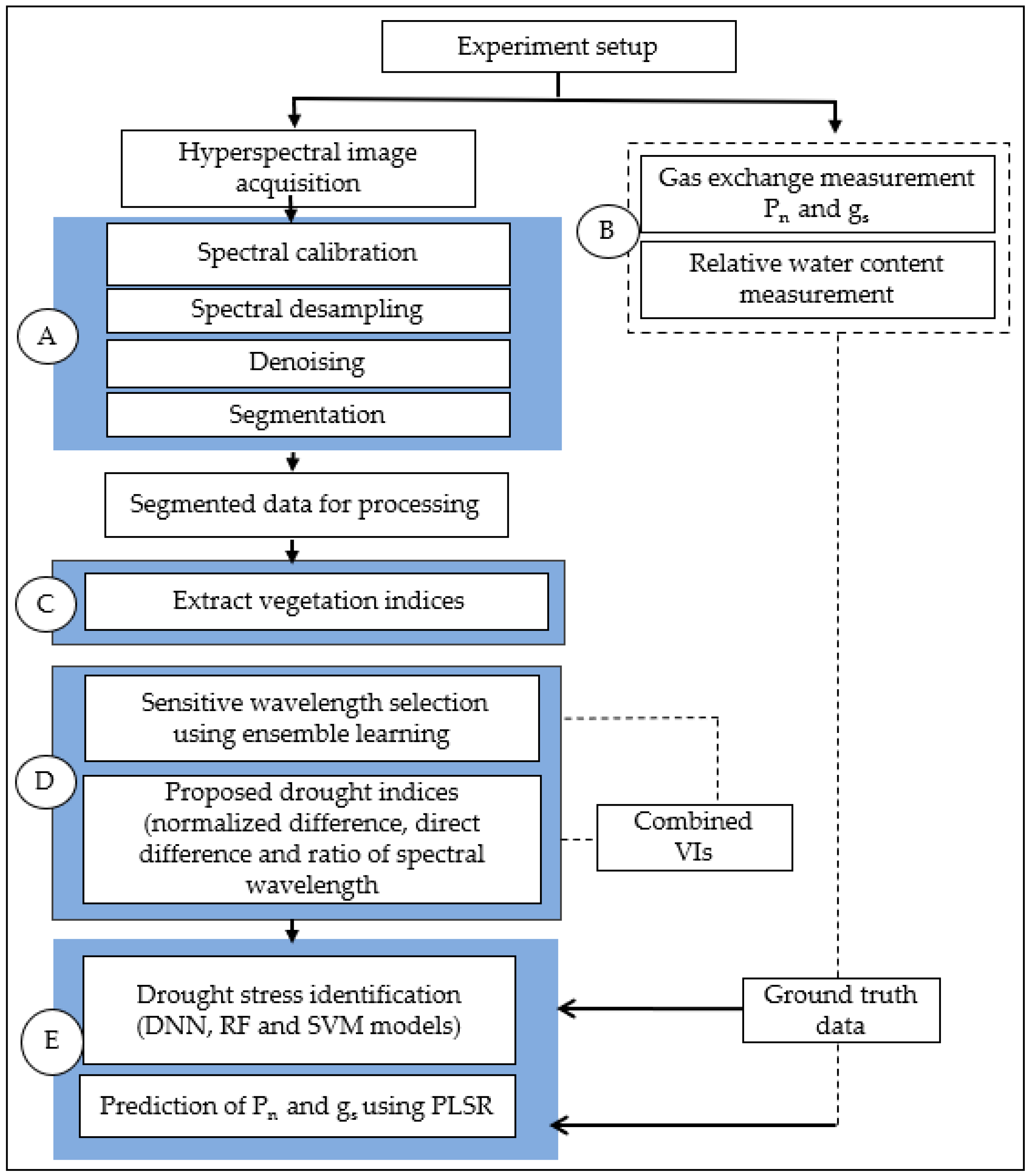
Figure 1 shows the workflow of the methods used in this experiment. The general steps include HSI acquisition, data pre-processing, selection of known VIs, sensitive waveband selection, development of proposed VIs, development of ML models, identification of drought stress, and prediction of Pn and gs.
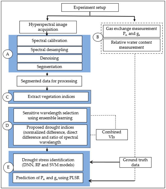
Figure 1.
The schematic diagram of the methodology for analyzing spectral images for drought stress identification (A) is the pre-processing step (involving data calibration, denoising, desampling, segmentation); (B) is the drought stress-related physiological measurements (photosynthetic rate (Pn), and stomatal conductance (gs)); (C) is the extraction of known VIs; (D) is the ensemble learning model for selecting sensitive spectral wavelengths; (E) is the development of classification and regression models for identification of drought stress and prediction of gas exchange measurements traits; Pn and gs.
2.1. Experiment Setup
A drought experiment was set up in a glasshouse facility (https://www.cranfield.ac.uk/facilities/plant-growth-facility, accessed on 10 November 2022) at Cranfield University. This facility has a state-of-the-art phenotyping platform (Lemnatec Scanalyzer system) for high-throughput data acquisition. In this experiment, a wheat cultivar, Cadenza, was planted in 8 cm by 6 cm pots filled with low-N peat soil (Levington Advance M3, CTS, BHGS Ltd, Worcestershire, UK). Plants were grown under natural light (with an average light intensity of 450–600 µmol/m2/s PAR) with a 20 C to 23 C day temperature range, while the optimum night temperature was between 18 C and 20 C. Plants (48 in number) consisting of four treatments and 12 replicates were arranged in a randomized complete block pattern. The treatments comprised plants with two N and water content levels: WWHN, WWLN, DSHN, and DSLN (WW = well-watered; DS = drought stress; HN = high N; and LN = low N). The plants were fertilized with two N levels, high N and low N, made of 42.5 mM and 4.25 mM concentrations, respectively, at 30, 37, and 44 DAS (days after sowing). They were prepared from a modified Letcombe nutrient solution [27]. For the drought stress treatment, all the plants were first watered with equal amounts of deionized water until the tillering stage (44 DAS), when the drought stress was imposed (0 DADS—day after drought stress). All the well-watered treatments (WWHN and WWLN) were kept at 80% field capacity (FC) (% FC is the proportion of soil moisture content at field capacity), while the watering was stopped for the drought stress treatments (DSHN and DSLN). The well-watered plants were watered slowly and thoroughly with deionized water each day until the soil reached the desired moisture level (80% FC). To ensure the WW plants were at 80% FC or above, a portable soil moisture meter was used to measure the volumetric soil water content daily. In addition, the pots were weighed daily to determine the rate of water decrease in the DS-based treatments. The soil surface was covered with white pebbles to minimize water loss through evaporation. The WW plants were watered daily until the end of the experiment, which lasted for 15 days.
2.2. Physiological Measurements of Drought Stress
Drought stress can significantly affect the gas exchange rate of plants, reflecting plant physiological responses to low water content. Gas exchange measurements such as stomatal conductance (gs), transpiration rate, and photosynthetic rate (Pn) are often used to track changes in the physiological properties of plants before noticeable symptoms such as yellowing or wilting become apparent [28]. This study used the gs (mmol H2O m−2 s−1) and Pn (µmol CO2 m−2 s−1) of plants as ground truth measurements to track changes in plant physiological traits resulting from drought stress and N deficiencies. Stomatal conductance measures the rate at which CO2 or water vapor enters and exits through plant stomatal pores. It is a critical physiological indicator for screening drought-tolerance genotypes of plants [29]. Additionally, the photosynthetic rate represents the capacity of plants to convert carbon dioxide into organic compounds [30].
A LI-6400XT portable photosynthesis system (LI-COR Biosciences Inc., Lincoln, NE, USA) was used to measure the gas exchange measurements of the plants a day before the water stress was induced and continued every three days until the end of the experiment. Stomatal conductance measurements were made between midday and 1700 h on the fully expanded leaf of the main stem that had been marked and tagged. The CO2 concentration in the leaf chamber was fixed at 400 μmol CO2 mol−1. To achieve the maximum photosynthetic capacity, the leaf flow rate, temperature, relative humidity, and photosynthetically active radiation were set at 200 µmol s−1, 20 °C, 50–65%, and 1800 µmol m−2 s−1, respectively. The stomatal conductance values were recorded once the measurement was stabilized. The leaf area was corrected during data processing when the leaf was smaller than the cuvette of the chamber.
To analyze the effects of each treatment on the dynamics of the gas exchange measurements, the average gs and Pn of each treatment were subjected to a one-way ANOVA test followed by Tukey’s honest significant difference (HSD), with * p < 0.05 considered statistically significant. The ANOVA test compares the means across multiple groups to determine if there exist any statistically significant differences between them. The statistical analysis was performed in RStudio (Ver. 1.1.414, RStudio, Boston, MA, USA).
2.3. Hyperspectral Data Acquisition
The Lemnatec Scanalyzer housing a hyperspectral camera (hyperspec® inspectorTM Headwall Photonic, Headwall Bolton, MA, USA) in the glasshouse was used to acquire spectral images 3 m above the ground. The camera is a push broom type that covers the visible-and-near-infrared (VNIR) regions, collecting light reflections between 390 nm and 1015 nm through an imaging slit. As the sensor is in motion, one row of spatial pixels is collected per frame, where each pixel is made of the corresponding spectral data. The sensor uses an FWHM (full width at half maximum) image slit of 2.5 nm to gather data at 0.7 nm (in the VNIR area). It has 1600 × 1800-pixel spatial resolution and 925 spectral information with an f/2 optical aperture. The sensor is directed vertically downward to the ground, scanning 6 pots (50 cm apart) in a row at each pass. Spatial images are created by concurrently capturing the spectral information of pixels distributed along the scan line while the mirrors move horizontally. The target is scanned line by line, and spatial images are formed by recording simultaneously the spectral information of pixels distributed in a scan line (across-track direction), while the mirrors move horizontally. For information on the operation and use of the Head photonic sensors for hyperspectral data acquisition, readers are referred to [31,32,33] for further details. Imaging began on the day the drought was induced and continued every other day until the end of the experiment. This produced a total of 252 sets of hyperspectral imaging data.
2.4. Hyperspectral Image Pre-Processing
Obtaining useful information from hyperspectral images requires pre-processing to normalize the spectral data from ambient illumination, reduce noise and other artifacts, and improve the data quality for further processing. The pre-processing steps include radiometric calibration, spectral down-sampling, and noise removal. Radiometric calibration standardizes and adjusts the radiometric data recorded by converting the raw sensor measurements to meaningful physical units such as radiance or reflectance. This is important in reducing the variable illumination and the dark current effect on the spectra. In this study, a white panel (Zenith Lite™ Ultralight Targets 95%R, Sphereoptics®) was imaged as the white reference data ( while the camera lens was covered with an opaque cap to collect the dark reference data () [34]. The image reflectance was obtained by using Equation (1).
Hyperspectral imaging captures high-resolution images across a wide range of narrow and continuous spectral bands. The massive amount of information presents computational challenges that require down-sampling of the data for effective processing. Down-sampling involves reducing the number of spectral bands or channels in the data, subsequently reducing the spectral resolution. According to Sadeghi-Tehran et al. [32], down-sampling helps reduce the computational complexities and noise generated during hyperspectral data acquisition. This study used a band-averaging technique of 2 nm spectral width to down-sample the data. The process involves grouping two adjacent spectral bands and finding the average values to generate a new set of bands. As a result, the down-sampled data had fewer wavebands overall but still had a representative spectral characteristics.
Spectral smoothing and denoising methods were applied to the raw spectra to reduce noise levels and improve the signal-to-noise ratio, revealing underlying spectral patterns. Spectral smoothing and denoising include using filters on the spectral bands to remove spikes and smooth spectral curves. This process also isolates sensitive features that could be masked by noise at various wavelengths. Here, a Savitzky–Golay filter (a commonly used low-pass filter) to smooth and denoise the spectral bands was used to fit a polynomial function to the data inside a moving window as a form of polynomial smoothing. The filter chooses an odd-sized window of spectral points for each data point in the spectrum and then fits the least square using the high-order polynomial. During this process, the relevant data points are eventually swapped out for the matching values of the fitted polynomial. A window of size 13 and a second-degree polynomial were used as the parameters. It should be noted that a small window size generates significant artifacts, while a large window size can be more effective in reducing large-scale noise and smoothing out noise of variable frequencies. However, large window sizes tend to blur fine spectral details, which could distort the originality of the spectral signature [35].
2.5. Segmenting the Hyperspectral Data
After pre-processing, the HSI data were segmented using a selected spectral ratio and Otsu thresholding. A method that exploits the difference in the shape of the infrared red regions of the spectrum in the plant and background was developed for the spectral ratio. In this case, a normalized difference ratio between 910 and 950 nm wavelengths was extracted to create the spectral ratio. The combination of spectral ratio and the Otsu thresholding resulted in a binary image where the vegetation pixels were labeled as one and the non-vegetation pixels as zeros. Supplementary Figure S1 shows the original image and its corresponding image of a sample of the hyperspectral data.
2.6. Extracting Known Vegetation Indices
Vegetation indices (VIs) of plants derived from reflectance values in specific bands are indicative of responses to different stresses. Combining VIs or customizing them based on unique vegetation characteristics and environmental conditions is a common practice to monitor plant stress [36]. This study extracted twenty-five known VIs sensitive to nitrogen variations and drought stress (Table 1). The top ten VIs that correlated well with the gas exchange measurements were evaluated to understand their sensitivities to subtle changes in the nitrogen and water content of plants. The selected VIs were used subsequently for the subsequent analysis.

Table 1.
List of selected VIs to monitor plant drought stress.
2.7. Wavelength Selection and New Drought Stress Indices
Wavelength Selection Using Ensemble Learning
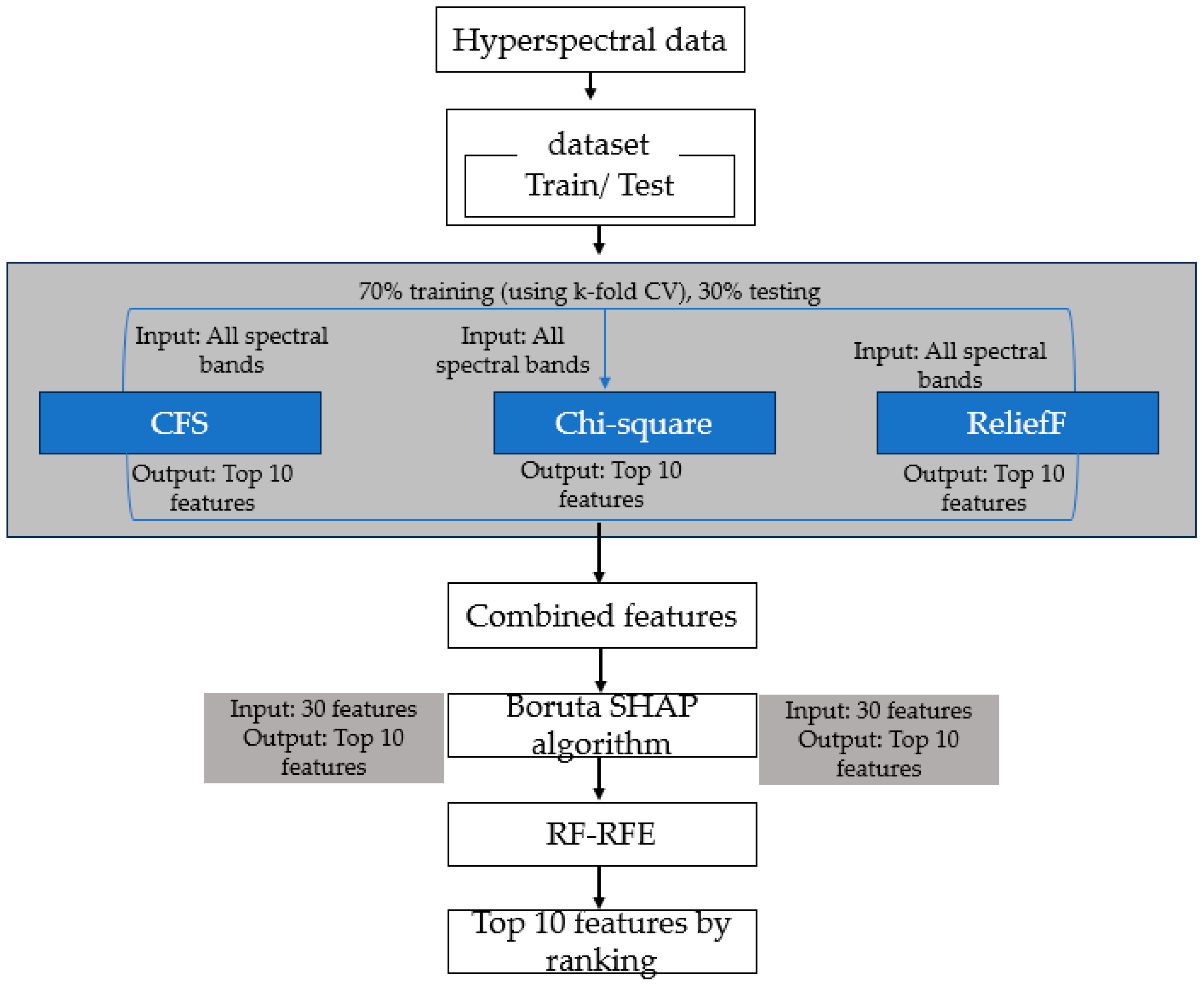
Hyperspectral images have a high spectral resolution comprising hundreds of narrow bands. However, a significant portion of the spectral bands may be strongly correlated (multicollinear). To reduce this multicollinearity, sensitive features related to the phenotypic traits of interest are extracted using machine learning and statistical methods [53]. This study implemented an ensemble learning method to select the most sensitive features (Figure 2). Three feature selection models, correlation feature selection (CFS), chi-square (CS), and ReliefF (RFF) were developed on 70% of training datasets and tested on 30% of test datasets. Each model was trained using a k-fold cross-validation technique where the training dataset was divided into K (5) subsets to train and validate the model multiple times. The features selected were ranked in order of importance, and the top ten features from each model were selected. Because each model had its drawbacks, the feature subset that was ultimately selected might not be the best in the feature space. The features selected were combined to obtain 30 features. A further selection was made on the combined feature subset using a Boruta SHAP algorithm [54], which was ranked using a recursive feature selection method.
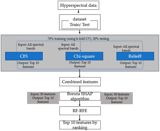
Figure 2.
Workflow of the ensemble feature selection pipeline.
The selected wavelengths were used to develop new indices: drought-N ratio index (RDI), normalized difference drought-N index (NDDI), and drought difference index (DDI) using Equations (2)–(4). These equations were selected because they help minimize the effect of varying light conditions, including sunlight intensity, angle of sunlight, etc., on the plant reflectance measurements. Additionally, the indices from these equations reduce the effects of atmospheric conditions such as haze, aerosols, and scattering on plant reflectance [55].
where and are any two selected wavelengths.
Using a custom-developed algorithm, the three proposed indices were calculated for every possible pair combination of the selected wavelengths. The relationship between the generated indices and the gas exchange measurements was ascertained using correlation analysis. A matrix plot displaying a distinct pattern with multiple hotspots with somewhat varied coefficient of determination (R2) values were produced by plotting all the squares of correlation coefficient r values, which reflect the coefficient of determination. The optimal wavelength combinations with the highest R2 values were chosen as the proposed indices.
2.8. Machine Learning Models for Drought Stress Identification
Three machine learning algorithms, SVM, RF, and DNN, were trained using the selected known VIs, proposed VIs, and combined VIs (combination of known and proposed Vis) to identify drought stress in wheat. All three models are supervised learning models for both classification and regression tasks. SVM finds the optimal hyperplane that maximizes the margin between classes in the feature space, while RF is an ensemble learning model [56] that uses bagging techniques where multiple decision tree models are trained on various subsets of data independently [57]. DNN consists of multiple layers of neurons (input, hidden, and output layers), with each layer containing numerous neurons connected through weighted to learn a hierarchical representation of data through a backpropagation algorithm [58]. Supplementary Table S1 shows a comprehensive characteristic of each model and the reasons for choosing the model for the identification of drought stress in wheat.
2.9. Multivariate Analysis for Stomatal Conductance and Photosynthetic Rate Predictions
Based on prior research, gas exchange measures can evaluate and track the dynamics of drought stress since minute changes in these physiological traits indicate responses of plants to water availability. However, the tools for measuring gas exchange are costly, low throughput, and sometimes destructive. Hence, regression models were developed to predict the plant gs and Pn using the plant VIs, which could be used as a proxy tool to monitor drought stress. Four models, a polynomial regression (PR), random forest regression (RFR), support vector regression (SVR), and partial least squares regression (PLSR), were trained to evaluate their abilities to predict gs and Pn. The RFR, SVR, and PR were each trained with the VIs as the independent factors, while the gs or Pn was the dependent variable. The PLSR model was computed considering the whole spectral reflectance as the independent variable and gs or Pn as the dependent variable. Here, the PLSR model was trained by concurrently finding the principal components that account for the highest variance and low multicollinearity in the dependent and independent variables [59]. This results in fewer uncorrelated components (variables) from the large spectrum with little loss of information.
2.10. Model Training and Testing
All the models were trained with 70% of the dataset and tested on the remaining 30%. In ML training, optimization of parameters by cross-validation (CV) search over various parameter settings is required to improve the accuracy of predictions and classification and minimize errors. Popular optimization techniques include gridsearchCV [60], randomized search [61], and Bayesian optimization [62]. Since random search is computationally less expensive and consumes less time for processing, the randomsearchCV tool in the Scikit learn package (Python 3) was used to fine-tune the parameters of the ML models. Table 2 includes the list of parameters tuned and the range of values considered. Following the model parameter tuning and training, the best-performing set of parameters was used for model fitting and classification or regression.

Table 2.
Model parameters for tuning and training using random search CV.
The metrics root mean square error (RMSE), coefficient of determination (R2), and mean absolute error (MAE), as shown mathematically from Equations (5) to (7), were used to assess the validity of the regression models in predicting the Pn and gs. The R2, ranging from 0 to 1, measures the proportion of the variance in the dependent variable that is predictable from the independent variables. R2 values close to 1 indicate a good fit, which shows a good performance of the model, and vice versa. The RMSE measures the square root of the average squared differences between the predicted and observed variables, which gives a sense of the magnitude of the errors made by the models. A low RMSE suggests a good performance of the model. Generally, a high R2 and low RMSE indicate good performance of the model. The MAE is the average of the absolute differences between predicted and observed variables. A lower MAE shows that the model’s predictions are close to the ground truth values. To objectively assess the performance of the classification models, we used three widely used classification metrics: average accuracy (AA), F-score, and Cohen’s kappa score, as shown in Equations (5)–(10)
where n is the amount of data, xi is the observed values, yi is the predicted values, and the bar denotes the mean of the variable. Statistical calculations were performed using the statistical package in RStudio.
where P = and R = ; TP: true positive; TN: true negative; FP: false positive; FN: false negative; Po is the probability of observed agreements; and Pc is the expected agreement.
3. Results
Before analyzing the results of the interaction between the proposed and known VIs and how they are affected by drought stress and variable N levels, it is important to understand how the multiple stresses affected the gas exchange measurements (which served as ground truth measurements for this study) and the whole spectra of each treatment. Section 3.2 summarizes the results of the plants’ gas exchange measurements under drought and various N levels, while Section 3.3 examines the spectrum characteristics of each treatment at three different growth stages. The following sections further detail the extraction and proposal of new VIs and how they respond to drought stress when combined with the known Vis.
3.1. Reference Data of Gas Exchange Measurements
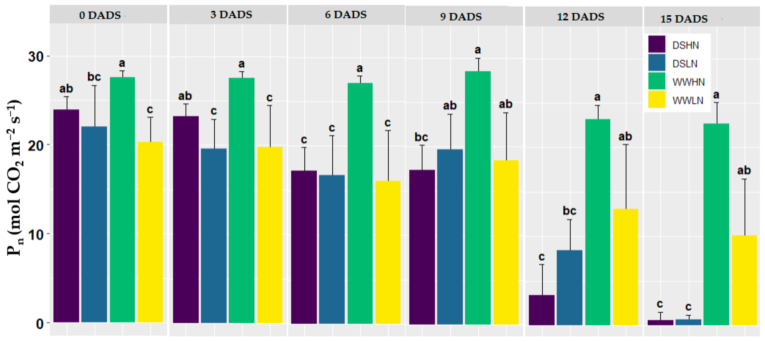
Figure 3 is a box and whisker plot of the Pn measurements of the plants from the 0–15 DADS. The WWHN treatment produced the highest Pn throughout the drought stages, while the DS treatments (DSHN, DSLN) steadily declined with time. It was observed that the DS treatments were not significantly different at the beginning of the drought (0 DADS), despite the variations in their N levels. However, the DSHN treatment was statistically different from the WWLN treatment. Plants with varying N levels exhibited statistical differences three days after drought stress initiation. That is, the WWLN and WWHN were statistically different (p < 0.049), while the DSLN plants showed differences with the WWHN (p < 0.045). The WWLN and DSLN, however, showed no differences at this stage. The stress in the DS treatments became more noticeable on the 6 DADS, where the means of both treatments (DSHN and DSLN) were statistically different from the WWHN treatment (p < 0.026 and p < 0.015 for DSHN and DSLN, respectively). In contrast, the WWLN did not differ much from the DSLN (p < 0.97) treatment; however, it was statistically different from the WWHN (p= 0.036). At the end of the experiment, there were clear distinctions between the drought-stressed (DSHN and DSLN) and well-watered (WWHN and WWLN) treatments.
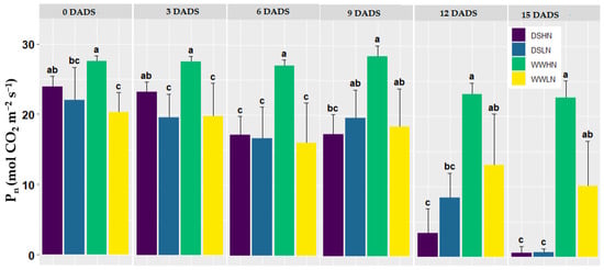
Figure 3.
Photosynthetic rates from 0 to 15 DADS for four different treatments: WWHN, WWLN, DSHN, and DSLN. The WWHN and WWLN are the water well-watered plants with high and low nitrogen, respectively, while the DSHN and DSLN are the drought-stressed plants with high and low N levels, respectively. The results presented are mean and standard deviations from the original data; the dissimilar lower-case group (a, b, and c) represents a significant difference with p < 0.05.
The gs measurement of the plants revealed a pattern comparable to the Pn measurement, as shown in Figure 4. Throughout the drought stages, the WWHN treatment had the highest gs, with the maximum at six DADS (0.37 mol H2Os−1). Despite having varying N levels, the DS treatments showed no significant differences at 0 DADS. At 0 DADS, the means of the DS treatments (DSHN and DSLN) were statistically different from the WWLN treatment. After three days, the WWHN treatment had the highest gs (0.341 mol H2Os−1), while the DSLN obtained the lowest gs (<0.252 mol H2Os−1). There were observable differences in the ranges and mean values of the WWHN treatments and the other treatments, with p-values = 0.025, 0.011, and 0.012 for the WWLN, DSLN, and DSHN treatments, respectively. However, the DS treatments were not significantly different from the WWLN. On the six DADS, the WW treatments (WWHN and WWLN) had higher mean gs than the DS treatments. While the DS treatments were statistically different from the WWHN treatment, the DSLN and WWLN treatments were statistically not different. On the 12 DADS, there were 80.3% and 60.2% decreases in gs for the DSHN and DSLN, respectively (indicating a fast decline of gs for the DS treatments). On the final day (15 DADS), a significant difference was observed in drought-stressed and well-watered plants, with the WWHN having the highest and the DSHN having the lowest gs measurements.
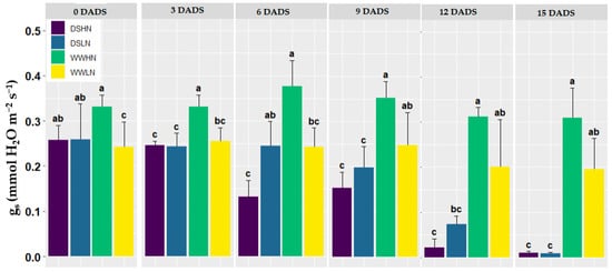
Figure 4.
Stomatal conductance for the four treatments: WWHN, WWLN, DSHN, and DSLN from 0 to 15 DADS. The WWHN and WWLN are the water well-watered plants with high and low nitrogen, respectively, while the DSHN and DSLN are the drought-stressed plants with high and low N levels, respectively. The results presented are mean and standard deviations from the original data; the dissimilar lower-case group (a, b, and c) represents a significant difference with p < 0.05.
3.2. Spectral Reflectance Analysis
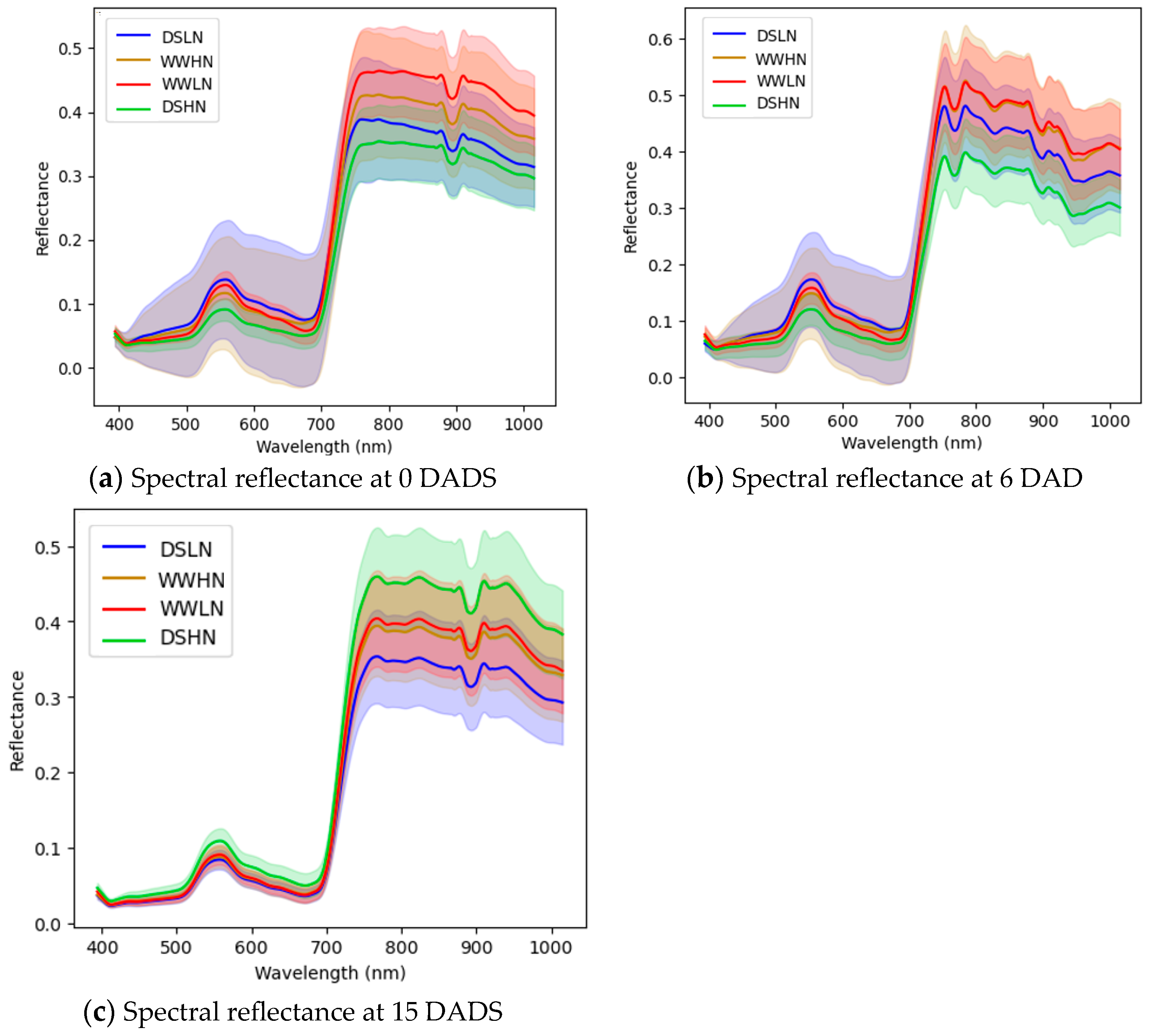
Mean spectral curves for the different treatments at 0, 6, and 15 DADS are shown in Figure 5. The spectral curves for all the treatments showed peaks at 570 nm and troughs at 680 nm. The spectral reflectance of all the treatments exhibited comparable patterns at 0 DADS, showing relatively low reflectance, particularly in the blue spectrum (around 450 nm) and red regions (around 670 nm). However, the DSLN treatment had slightly higher reflectance comparably. The red edge region (around 700 nm) for all the treatments showed a sharp progression from the red to the near-infrared regions, with the high N treatments (DSHN and WWHN) showing a relatively higher reflectance in this region as compared to the low N treatments, which showed low reflectance. Conversely, on the 6 DADS, the general trend in the visible spectrum was similar for all the treatments with low reflectance in the blue (~450 nm) and red (~670 nm) regions. In the red edge region, the WWHN had the highest reflectance (0.57 at around 730 nm), while the DSHN had the lowest reflectance (0.39 around 720 nm). All the treatments had a slightly downward trend in the reflectance value in the near-infrared regions. Furthermore, reflectance’s for the well-watered plants (WWLN and WWHN) were close in proximity, with WWHN showing slightly higher reflectance in the near-infrared regions. On the final day of the experiment (15 DADS), all the treatments showed relatively low reflectance with minor variations, with the DSHN treatment showing a relatively high reflectance (0.11) in the visible region. All the treatments showed a sharp increase in reflectance in the red edge region starting around 680 nm and transitioning to the near-infrared regions. However, the DSLN had a slightly less sharp and shifted shape in this region. Interestingly, the DSLN had the highest reflectance in the near-infrared region.
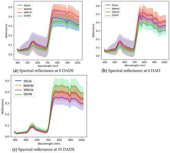
Figure 5.
Spectral reflectance of the averaged DSHN, DSLN, WWHN, and WWLN treatments for 0 DADS (a), 6 DADS (b), and 15 DADS (c). Spectral values are shown as mean ± standard deviation. The WWHN and WWLN are the water well-watered plants with high and low nitrogen, respectively, while the DSHN and DSLN are the drought-stressed plants with high and low N levels, respectively.
3.3. Correlation between the Known VIs and Gas Exchange Measurements (Pn and gs)
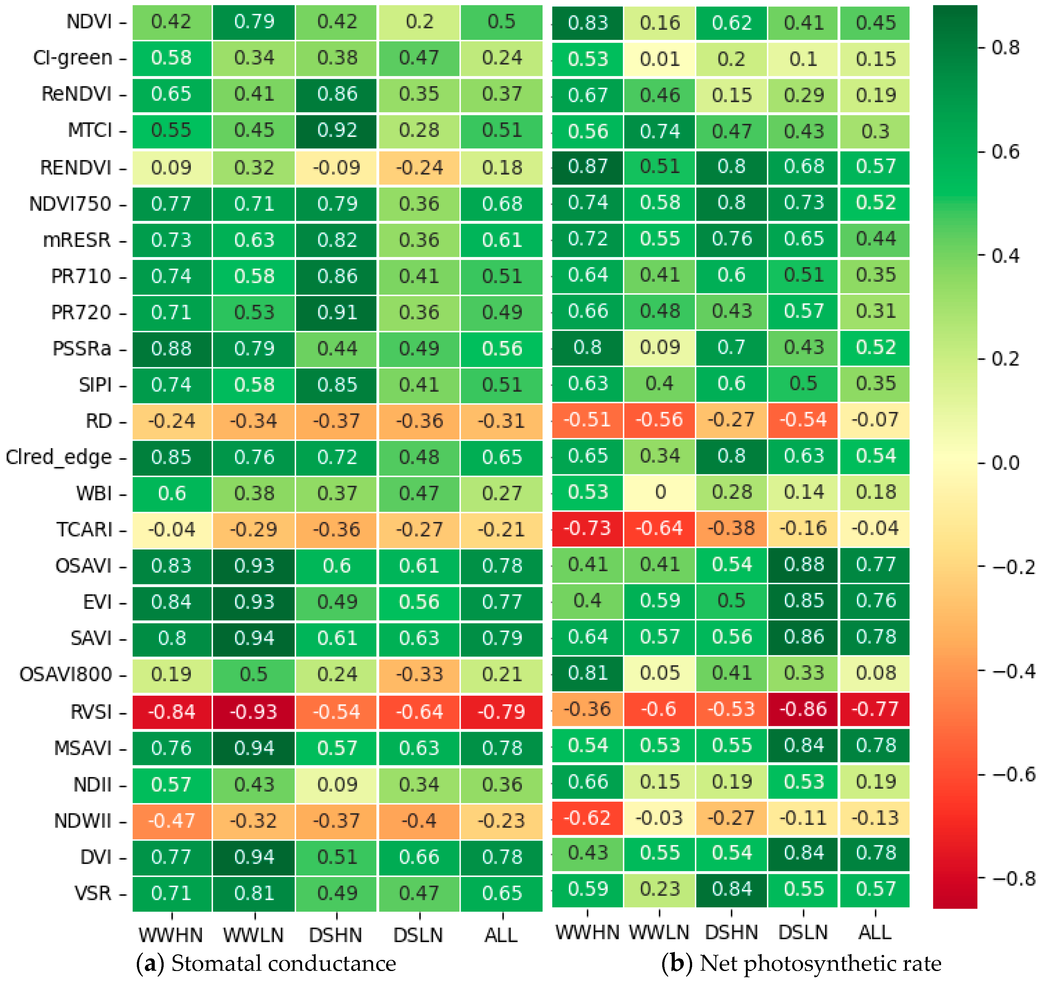
Figure 6 displays heat maps of the Pearson correlation coefficient (r) between the known VIs and the two gas exchange variables (Pn and gs). The correlation analysis was performed for each treatment and the combined treatments (ALL). Figure 6a shows good relationships between the VIs and gs in the WWHN treatment. PSSRa had the highest correlation coefficient (0.88), while TCARI obtained the lowest (−0.04). Similarly, most VIs had strong correlations in the WWLN treatment, with DVI, SAVI, and MSAVI obtaining the highest correlation coefficient (0.94) and TCARI with the lowest (−0.29). However, a contrasting trend was observed in the DS-based treatment. With the DSHN, while the MTCI with r = 0.92 had the best correlation with the gs, a third of the extracted VIs had a poor relationship with the gs (r < 0.4). The DSLN treatment reported the lowest correlation with the gs measurements. SAVI (0.79) and RSVI (−0.79) were observed to have the highest correlation, while NDVI (0.20) had the lowest correlation with the gs. When the treatments were combined, most of the known VIs showed a positive correlation with the gs except NDWII, RVSI, TCARI, and RD indices. The RVSI and SAVI had the highest correlation coefficients (−0.79 and 0.79, respectively), and the NDVI800 had the lowest (0.18).

Figure 6.
Pearson correlations between the extracted features and the gas exchange measurements (Pn and gs). VIs with a correlation of more than 0.5 were selected for further analysis. See Table 1 for abbreviations of VIs.
From Figure 6b, a positive correlation was observed between the known VIs and the Pn measurements in the WWHN treatment, except for a few indices (NDWII, RVSI, TCARI, and RD), which were negatively correlated. Most indices had a high correlation coefficient, with RENDVI (0.87). The results obtained for the WWLN treatment show that compared to the WWHN, there was a relatively low correlation between the indices and the Pn measurements. MTCI had the best correlation (0.74) while the NDWII (−0.03) had the lowest. In the DSHN treatment, the VSR index obtained the highest correlation coefficient (0.84) and the NDII (0.19) had the lowest. Unlike the gs, the indices in the DSLN treatment had relatively good correlations with the Pn. The highest correlation was observed in the OSAVI index (0.88), while the lowest was recorded in the CI_green index (0.10). With the combined treatments, the MSAVI, SAVI, and DVI reported the highest correlation with the Pn (0.78), while the RD had the lowest correlation (−0.07).
3.4. Waveband Selection and Proposed Indices
3.4.1. Spectral Band Pair Correlation
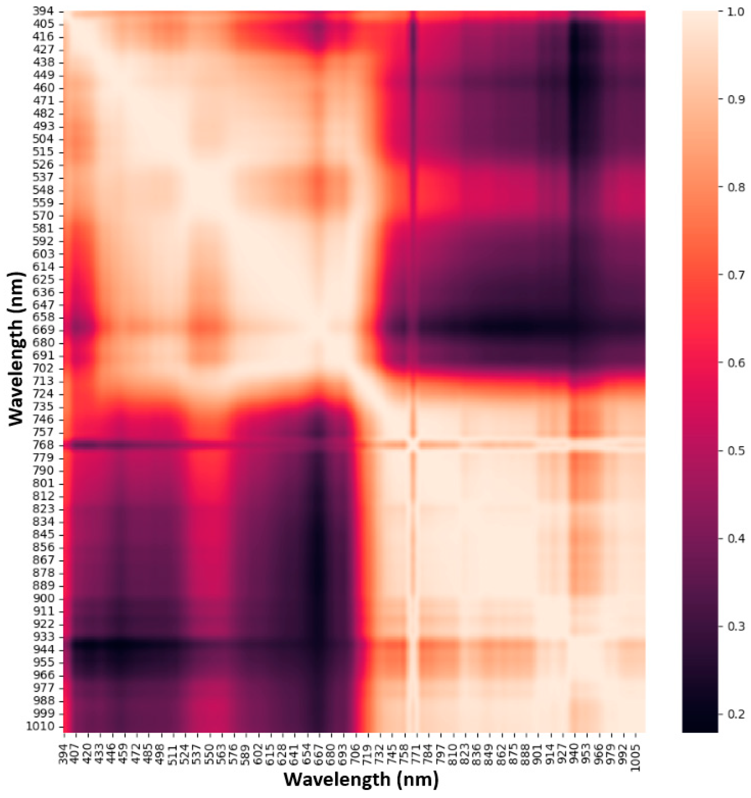
Spectral band pair correlation is the correlation analysis between two specific spectral wavelengths. It aids in understanding the interactions of different spectral bands, providing insights into the characteristics of the observed traits. In HSI data, a significant portion of the spectrum suffers from multicollinearity, which refers to the presence of strong correlations or dependencies between spectral wavelengths in a hyperspectral dataset. Figure 7 is a colormap showing the correlation between all pairs of wavebands of the data, providing a visual representation of how spectral features across a wide range of wavelengths are interrelated, indicating potential areas of redundancy or key spectral. The lighter color bands across the colormap suggest that certain wavelength ranges have high correlations with each other, while darker regions indicate lower correlations, suggesting that spectral features in these areas do not share much information or are not related linearly. The patterns off the diagonal (away from the central diagonal line) represent cross-wavelength correlations. Large blocks of uniform color off the diagonal indicate that features at one wavelength range are consistently correlated with features at another range. It is observed that the band pair correlation within the NIR region (700–1015 nm) follows a general pattern: adjacent bands had a strong tendency to correlate with one another. For example, around 394–450 nm, 740–790 nm, and 920–1015 nm, there are regions where spectral features are strongly correlated. However, among the highly correlated spectral bands in this region, a few bands had low correlations with their adjacent bands (940–953 nm). Spectral bands within the visible range (394–650 nm) had a low correlation between adjacent wavebands. However, bands between 511 nm and 576 nm were highly correlated to each other and to bands between 702 nm and 746 nm, showing the redundancy of some of these spectral features.
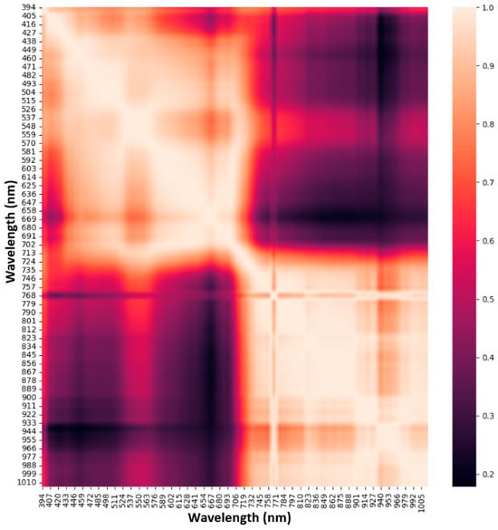
Figure 7.
A colormap image of the correlation between all pairs of spectral features from 394 to 1015 nm.
3.4.2. Output of the Ensemble Model Waveband Selection
Feature selection is critical in hyperspectral imaging analysis to enhance model performance by reducing overfitting, interpretability, and computational complexity [36]. The high correlation between the different spectral wavebands shows the significance of feature selection in eliminating redundant information while keeping the relevant data. Each model in this study selected the sensitive spectral features based on the order of importance. Table 3 reports the top ten spectral wavelengths selected by the ensemble model. The chi-square method selected most of the top features within the green spectrum from 555–570 nm and the rest within the red regions (670–675 nm). The top ten features using the ReliefF method were within the red (674–690 nm), red edge (722 nm), and infrared (949–957 nm) regions. The CFS selection method identified the top ten features within the green regions (542–547 nm), the red region (669–671 nm), and the infrared regions (939–957 nm). Generally, all three selection methods identified wavelength 674 nm as one of the most informative features. Also, the ReliefF and CFS identified 669, 949, 940, and 957 nm as the most sensitive features.

Table 3.
The top 10 wavelengths selected by the different machine learning models.
The output of the individual models was integrated with the Boruta SHAP model to improve the selection process and reduce the dimensions of the selected features. The output of the Boruta model was ranked in order of importance using the RF-RFE model. The ReliefF model ranked wavelengths in the green region as the top two (553 nm and 557 nm), followed by the red wavelengths (669 nm and 674 nm). Wavelength in the near-infrared region followed as the fifth most important feature. The 542 nm wavelength was selected as the tenth most important feature.
3.4.3. Proposed Drought Stress Indices
The selected wavelengths were combined in different forms using the RDI, NDDI, and DDI equations to obtain the proposed drought stress indices. To analyze the relationship between the drought stress and the proposed indices, the indices with high R2 values were selected. From supplementary information (Table S2), the NDDI and RDI produced the best indices that correlated highly with the gas exchange measurements (Pn and gs). Figure 8 is a correlation heatmap showing the relationship between the top ten proposed indices and the gas exchange measurements (Pn and gs). Based on the R2 values, the NDDI with wavelengths ( and ) had the best correlation for Pn (r = −0.78), whereas RDI with wavelengths ( and and ), and NDDI with wavelengths ( and ) produced the best correlation (r = 0.67) with gs.
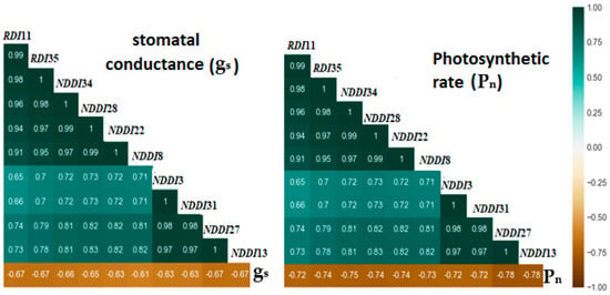
Figure 8.
Correlations between the proposed indices and the Pn and gs measurements.
3.5. Machine Learning-Based Drought Detection
This section evaluated the performance of the three traditional classification models (RF, SVM, and DNN) on identifying plants with drought stress with different nitrogen levels. Four different training features were used: known VIs, proposed VIs, combined VIs (proposed and known VIs), and PCA-transformed features. The performances of the models were evaluated based on the type of training features used.
3.5.1. Drought Stress Identification Using Machine Learning Models
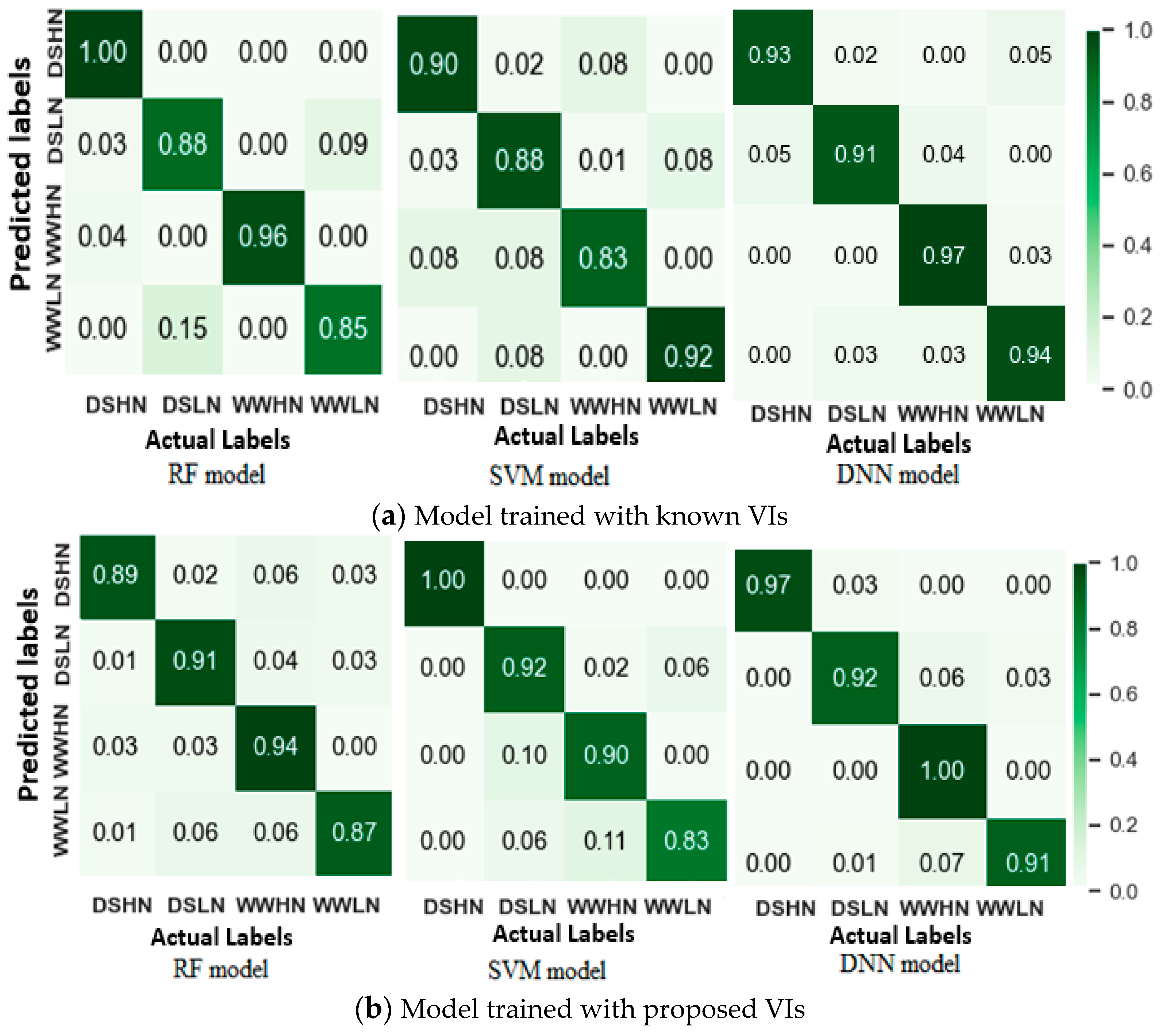
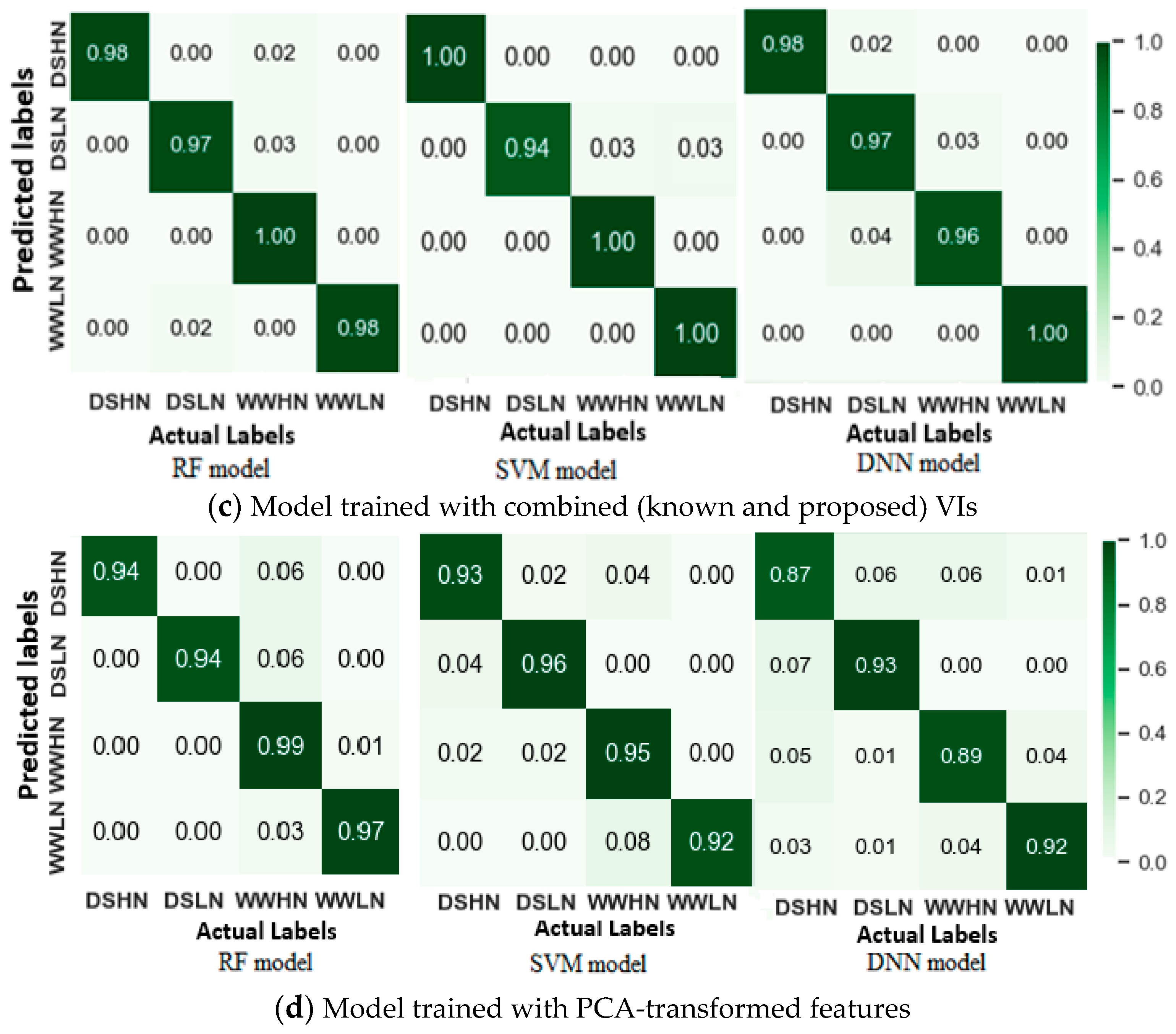
Table 4 shows the performance of the models when trained with the known, proposed, combined Vis and PCA extracted features. Figure 9 depicts the confusion matrices of the three models on the test dataset. This depicts the performance of the models in classifying the treatments: WWHN, WWLN, DSHN, and DHLN, which correspond to the different nitrogen and drought stress levels. The confusion matrices are displayed as heatmaps, with the classification accuracy increasing with the depth of color. The number of predictions made by the model for each class is shown by the cells in the heatmap. The x-axis shows the actual class, while the y-axis displays the predicted class.

Table 4.
Performance metrics for RF, SVM, and DNN models for identification of drought-stressed plants (metrics include average accuracy (AA), F1-score, and Kappa score).
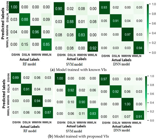
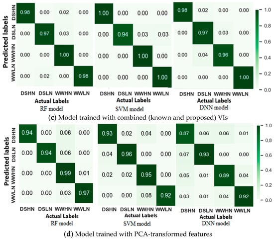
Figure 9.
Confusion matrices depicting the performance of the SVM, RF, and DNN classifiers trained with (a) known VIs, (b) proposed VIs, (c) combined Vis, and (d) PCA-transformed features.
Figure 9a shows the performance of the various models trained with the known Vis, with the DNN model showing the best results. All the models had high accuracies in identifying the high N-based treatments (DSHN and WWHN), with the RF model achieving a perfect accuracy score for the DSHN treatment identification. However, the SVM model had low accuracy for WWHN treatment. For drought-stressed plants in low N-based treatments, particularly DSLN, increased misclassification of treatments was observed. All the models had high F1-scores and above 0.80 Cohen kappa scores, which shows good agreement between predicted and actual class labels. The study demonstrates a performance improvement in the SVM and DNN models when trained with the proposed models, with the DNN achieving the best performance (Figure 9b). The SVM and DNN had a perfect accuracy score for WWHN and SVM while having low misclassification for other treatments. A high F1-score (0.911) and relatively low Kappa score (0.881) for the RF model shows that the model has resulted in false positives in contrast to false negatives for classifying the treatments. From Figure 9c, all the models performed well when trained with the combined Vis, as evidenced by the high percentage of correctly predicted cases in the diagonal elements of the confusion matrices. The RF model performed best, followed by the SVM and DNN models. However, a one-way ANOVA test on the F1-scores shows no significant variation in the performance of the models (Supplementary Information, Table S3). However, all the models showed comparably high misclassification for drought-based treatments. From the confusion matrices in Figure 9d, the three models had above 87% accuracy when trained with the PCA-transformed features. The RF model outperformed the others, producing above 0.90 accuracy scores in all four classes. However, it struggled to identify DSHN, as 6% of the treatment was classified as WWLN. The SVM model followed the RF model, recording the best performance in DSLN classification with a 4% misclassification error.
3.5.2. Multivariate Model Analysis for Stomatal Conductance and Photosynthetic Rate Predictions
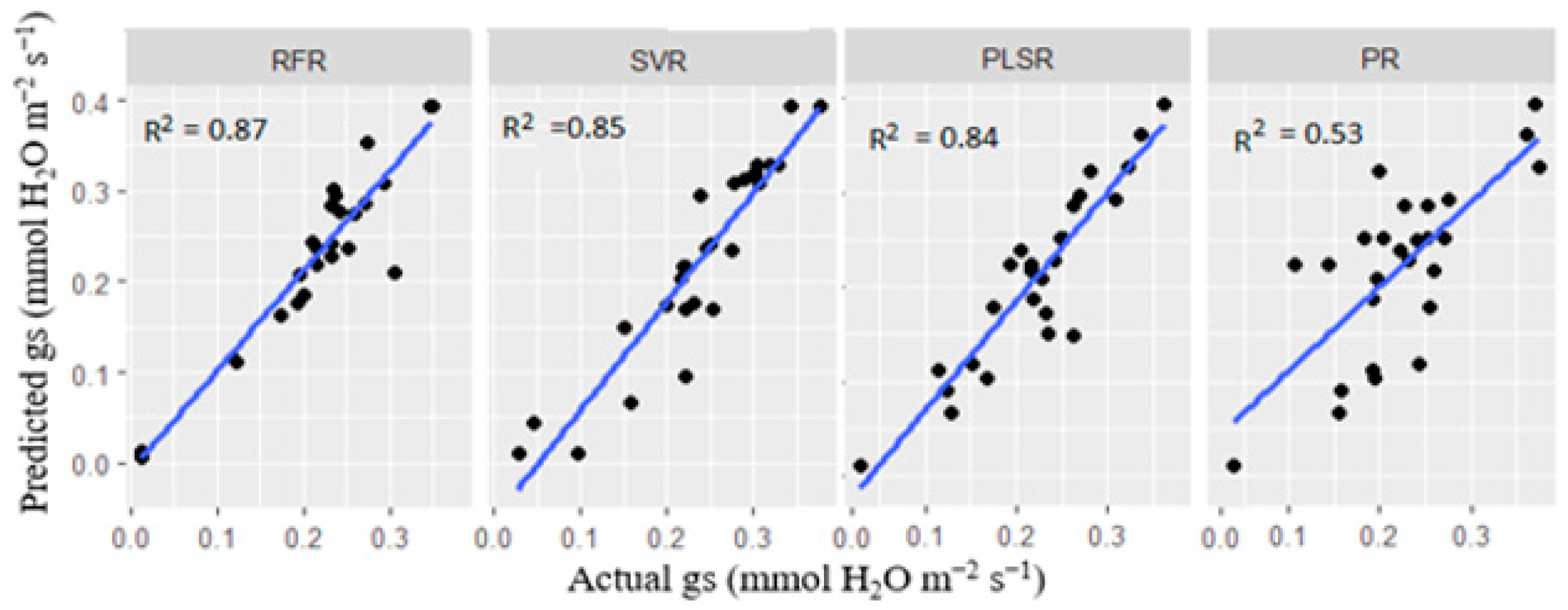
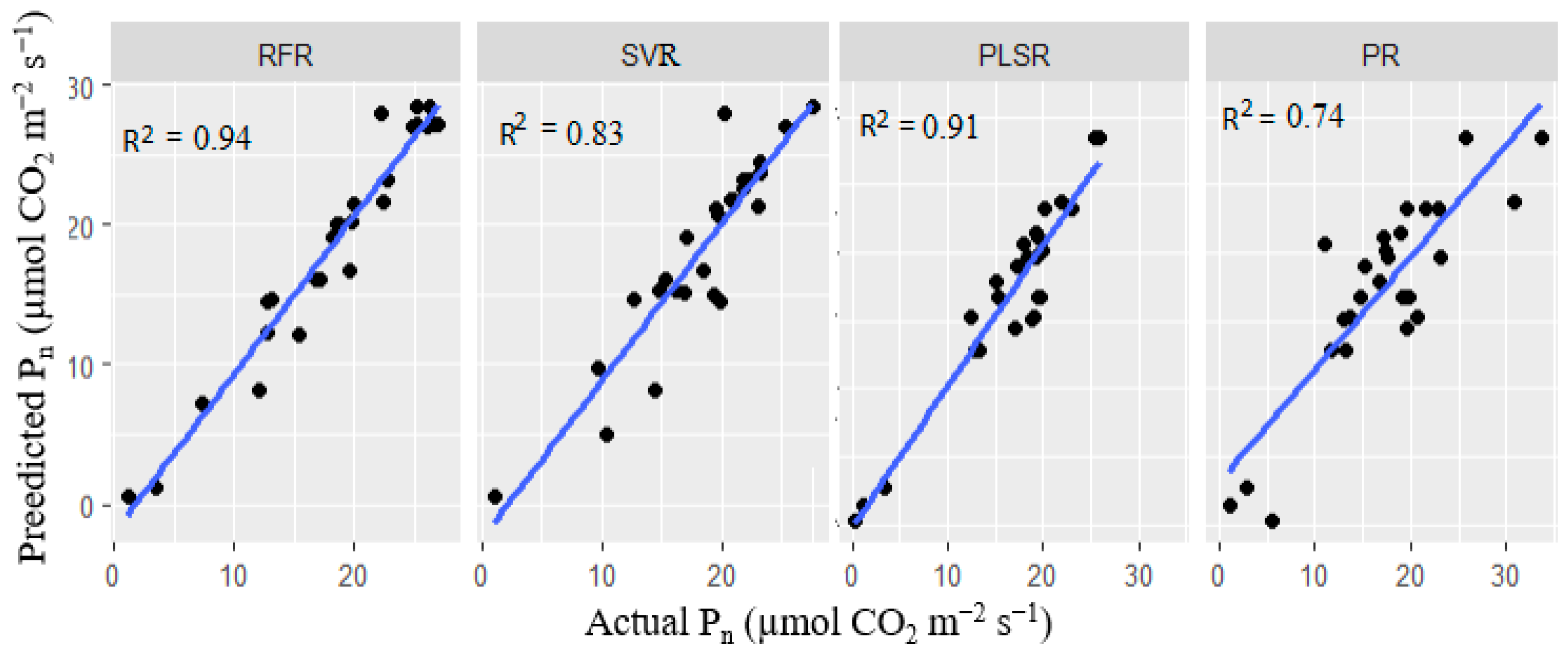
Figure 10 and Figure 11 are scatter plots illustrating the relationship between the actual and predicted gs and Pn. Table 5 also summarizes R2, RMSE, and MAE, depicting the performance of the regression models. It was observed in Figure 10 that most of the models achieved high prediction accuracy, with the random forest regression (RFR) outperforming the others with R2 = 0.87, RMSE = 0.035, and MAE = 0.015. The high R2 and low RMSE suggest that the RFR model is robust and insensitive to noise. In contrast, the PR model with an average R2 of 0.53 and RMSE of 0.52 was the least accurate in predicting the gs values. During the PLSR modeling using the whole spectrum, optimal latent features were selected to train the model to avoid the curse of dimensionality. In this case, fewer latent variables with maximum R2 and minimum RMSE were selected. For the gs-based PLSR models, 20 latent variables were selected. The PLSR model exhibited a high prediction score with a mean R2 of 0.842 ± 0.02 for the test scores. Although the RFR and SVR were trained with a limited number of features (10 sensitive spectral features), their performances were as good as the PLSR model.
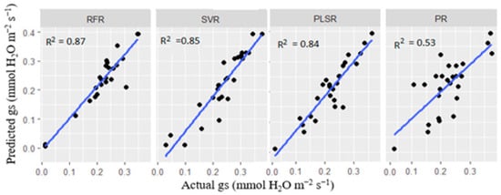
Figure 10.
Prediction of plant gs using four models (RF, SVR, PLSR, and PR). All the models were trained with the combined VIs except the PLSR, which were trained with the whole spectrum.
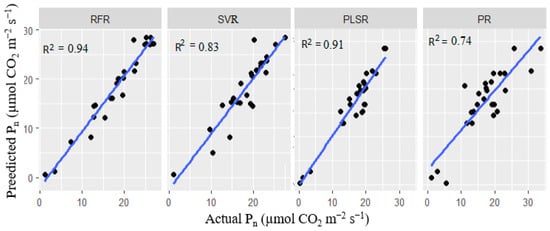
Figure 11.
Prediction of plant Pn using four models (random forest regression (RF), support vector regression (SVR), partial least square regression (PLSR), and polynomial regression (PR)). All the models were trained with the combined VIs except the PLSR, which was trained with the whole spectrum.

Table 5.
Performance of regression models for gs and Pn.
Figure 11 shows that all the models achieved considerably high performance in predicting the Pn values except the PR model, which had R2 = 0.74. The RFR model exhibited the highest score with R2 = 0.940 ± 0.05, RMSE = 0.015, and MAE = 0.004. Also, the PR model underperformed when trained with the combined VIs, achieving 0.740 ± 0.01 (R2), 0.144 ± 0.281 (RMSE), and 0.127 ± 0.04 (MAE). Similarly, to the PLSR model for predicting gs, 25 sensitive latent variables were selected for training the Pn-based PLSR model, which performed well with R2 = 0.910±0.04, RMSE = 0.015, and MAE = 0.004.
4. Discussion
This study utilized spectral information from hyperspectral imaging combined with different machine-learning models to identify drought stress in wheat species supplied with varying N levels. Since gas exchange measurements such as gs and pn are good indicators for drought stress monitoring, they were measured and analyzed in this study. From the results, the gs detected drought stress on the three DADS since the control group (WWHN) and the DS treatments significantly differed on this day. Drought stress was detectable on the six DADS using the Pn measurements, indicating the viability of using gas exchange measurements to track drought dynamics in wheat species. This supports the findings of [63], who analyzed the dynamics of plant water stress and recovery using the photosynthetic parameters, as gs and mesophyll conductance CO2 (gm), where the gs declined to 0.1 and less than 0.05 mol CO2 m−2 s−1 in moderately and severely water-stressed plants, respectively.
Analysis of the spectral curves of the hyperspectral data reveals differences in treatments in the visible and near-infrared regions. The low reflectance of all the treatments in the visible regions was expected due to the strong chlorophyll absorption of the plants. This agrees with multiple studies that stipulate that healthy plants have low reflectance in the visible region, while high reflectance is normally observed in chlorophyll-depleted plants [64,65]. Although the low N treatments had a relatively low N content, they could not cause high reflectance, probably because the plants had a high concentration of chlorophyll at the start of the experiments. Nitrogen affects the overall plant health and leaf cellular structure of plants, where adequate N content builds strong cellular structure while degraded structure is observed in the plants with low N. The treatments with high N (WWHN and DSHN) with a strong cellular structure scattered light more effectively, which was evidenced in high reflectance in the red edge regions. The red edge region for these treatments is because of the leaf internal structure, which caused a rapid transition from strong absorption in the visible region to strong reflectance in the NIR region [66]. The high reflectance of the DSHN and WWLN treatments in the visible regions on the six DADS could be attributed to the decreased leaf pigments caused by the drought stress and low N level, respectively, which affected the leaf chlorophyll content [67]. The DSLN showing a relatively low reflectance in the NIR region shows that plants under drought stress with low nitrogen experience significant stress, which leads to reduced NIR reflectance. The drought and low N levels causes a cellular structural degradation, leading to a low reflectance in the NIR region.
Twenty-five known VIs were extracted, with some VIs (RVSI, SAVI, NDVI705, NDVI750, and EVI) revealing high correlations with the two gas exchange measurements. From previous studies [68,69], some of these VIs are associated with plant N, which shows that these indices may not be effective for drought stress analysis. Hence, further analysis proposing drought spectral indices was performed. Due to the high dimensionality of HSI, spectral averaging and sensitivity analysis were performed to select the wavebands responsive to drought stress and nitrogen deficiency. Over 600 features were discarded during the feature selection process, revealing that a small subset of spectral features could capture a significant amount of the most valuable information. In contrast, most of the remaining features were typically redundant or contributed to noise [70]. The selection of sensitive spectral features in the red edge and green spectral regions shows the responsiveness of the wavelengths in these regions to both N variations and drought stress. Additionally, the selection and ranking of the 553 nm wavelength by the ensemble model as the most sensitive shows that it could decipher a physical meaning hidden in the high-dimensional spectral data of drought-stressed plants irrespective of the nitrogen level present.
The evaluation of the proposed VIs using a spectral combination of the sensitive features selected revealed that the NDDI and RDI-based indices had strong relationships with drought stress, with NDDI30 and NDI20 having the strongest R2 values of 0.78 and 0.69, respectively. The proposed indices were primarily derived from wavelengths in the blue (500, 550, and 580 nm) and near-infrared (710, 760, 770, and 783 nm) regions, which are reported as wavebands commonly used to measure drought stress and plant N status [71]. This finding is confirmed by the work of Colovic et al. [72], who identified the double difference index (DDI) produced from the near-infrared regions (749, 720, and 701 nm) as the best-performing index in explaining the variation in plant water levels. This shows the relatively important function of the near-infrared spectrum in drought stress analysis and that a single band might not be practical to evaluate plant health (drought stress) due to lant fluctuating nitrogen status and the dynamic nature of the drought stress.
Three models (SVM, RF, and DNN) were developed to identify stressed plants using the known VIs, the proposed Vis, and the combined VIs and PCA-transformed dataset. Generally, all three classifiers had outstanding performances. This shows that traditional machine learning models such as SVM and RF perform well in detecting drought stress in wheat species with the right feature selection. Although the models performed well when trained with the known or proposed VIs, their performance significantly improved when the two sets of VIs were combined. This could be because the combined VIs features cover the spectral areas strongly linked to both nitrogen and drought stress. For instance, indices such as OSAVI, RVSI, and NDDI30 are derived from the green and near-infrared regions, which strongly correlate to nitrogen concentration and drought stress. The PCA method reduced the dimensionality of the hyperspectral dataset (622 wavebands) to two feature sets representing the principal components. While PCA produces new feature components that maximize data variance, ignoring the lower-order PC components may have resulted in information loss, which affected the performance of the models [73].
Finally, while previous studies show that gas exchange measurements can monitor drought stress dynamics in plants, the process is costly and has low throughput. This study demonstrates the capability of training regression models using the combined VIs to accurately predict gs and Pn, as shown in Section 3.5.2; however, it is essential to note some limitations. The combined VIs were formulated from different spectral data, resulting in non-linear and complex data. Due to the non-linear and non-addictive nature of the data, the PR model was unable to learn the non-linear trend in the data.
This study contributes to the advancement of precision agriculture demonstrating the effectiveness of combined VIs with machine learning models for drought stress monitoring and gas exchange measurement prediction. The high accuracy in identifying stress despite the variable N levels shows the potential for precise and reliable stress monitoring. This study offers insights into the interactions between variable N levels and drought stress dynamics. The methodology has strong potential for large-scale application in agriculture, becoming a baseline for large-scale drought stress monitoring and management. This can enhance high crop yield by optimizing irrigation and nutrient application Although the study was conducted in a glasshouse, the scalability of hyperspectral imaging combined with machine learning modeling means that this method can be deployed in large-scale agricultural monitoring systems for high-throughput phenotyping.
5. Conclusions
In the field, crops can suffer multiple stresses, such as drought and nutrient deficiencies, affecting their yield and overall production cost. While these stresses have separate effects on plants, they also interact and have some common responses. Hence, identifying key traits to monitor drought-stressed plants at variable N status is crucial to improving crop yield. This study utilized spectral information from HSI combined with machine learning to identify drought stress and predict gas exchange measurements (gs and Pn) in wheat species. The experimental results demonstrated the capability of our proposed ensemble model in selecting spectral features that are highly responsive to drought dynamics in plants. A combination of the selected features resulted in proposed VIs, which achieved high accuracy in identifying the drought-stressed plants compared to using known VIs when used to train traditional machine learning models. However, the performance of the models improved significantly when tey were trained with a combination of proposed and known VIs, where DNN, RF, and SVM improved by 2.5%, 1.2%, and 1.8%, respectively, compared to the models trained with the known VIs. In addition to identifying drought stress by classification, the combined VIs were also used to train three regression models to predict gs and Pn measurements. The RF regression model outperformed the others in accurately predicting gs and Pn with error margins of 0.8 and 0.4, respectively. Although excellent results were obtained, more research is required to validate the conclusions on a larger spatial scale, exploring the potential application of the models for other plant species.
Supplementary Materials
The following supporting information can be downloaded at: https://www.mdpi.com/article/10.3390/rs16183446/s1, Figure S1: Pseudo RGB image9 (R: 650 nm, G: 550 nm, and B: 450 nm) and corresponding Segmented image (R: 600 nm, G: 500 nm, and B: 420 nm); Table S1: Machine learning models for the identification of drought stress in wheat under variable nitrogen levels. This shows the characteristics of each model and why they were chosen for this study; Table S2: Correlation coefficients of proposed indices with gs and Pn; Table S3: A one-way ANOVA test on the F1-score for all the models.
Author Contributions
Conceptualization, F.G.O. and D.K.C.; methodology, F.G.O.; software, F.G.O.; validation, M.J.H., F.M. and D.S.; formal analysis, F.G.O.; investigation, N.V. and L.G.; resources, M.C. and A.B.R.; data curation, F.G.O. and D.K.C.; writing—original draft preparation, F.G.O.; writing—review and editing, M.J.H., N.V., F.M., D.S. and L.G.; visualization and supervision, M.J.H. and F.M.; project administration, M.M.; funding acquisition, M.J.H. All authors have read and agreed to the published version of the manuscript.
Funding
This research was supported by the OCP S.A. under the University of Mohammed VI Polytechnic, Rothamsted Research and Cranfield University project (FP04). Rothamsted Research receives grant-aided support from the Biotechnology and Biological Sciences Research Council (BBSRC) through the Delivering Sustainable Wheat program (BB/X011003/1).
Data Availability Statement
The original contributions presented in the study are included in the article/Supplementary Material, further inquiries can be directed to the corresponding author.
Conflicts of Interest
The authors declare no conflicts of interest.
References
- Pirasteh-Anosheh, H.; Saed-Moucheshi, A.; Pakniyat, H.; Pessarakli, M. Stomatal responses to drought stress. In Water Stress and Crop Plants: A Sustainable Approach; Wiley: Hoboken, NJ, USA, 2016; Volume 1–2, pp. 24–40. [Google Scholar] [CrossRef]
- Duan, L.; Han, J.; Guo, Z.; Tu, H.; Yang, P.; Zhang, D.; Fan, Y.; Chen, G.; Xiong, L.; Dai, M.; et al. Novel digital features discriminate between drought resistant and drought sensitive rice under controlled and field conditions. Front. Plant Sci. 2018, 9, 492. [Google Scholar] [CrossRef]
- Xu, L.; Baldocchi, D. Seasonal trends in photosynthetic parameters and stomatal conductance of blue oak (Quercus douglasii) under prolonged summer drought and high temperature. Tree Physiol. 2003, 23, 865–877. [Google Scholar] [CrossRef] [PubMed]
- Leone, M. Advances in fiber optic sensors for soil moisture monitoring: A review. Results Opt. 2022, 7, 100213. [Google Scholar] [CrossRef]
- Grant, M.; Ochagavía, H.; Baluja, J.; Diago, P.; Tardáguila, J. Thermal imaging to detect spatial and temporal variation in the water status of grapevine (Vitis vinifera L.). J. Hortic. Sci. Biotechnol. 2016, 91, 43–54. [Google Scholar] [CrossRef]
- Zhang, Y.; Zha, Y.; Jin, X.; Wang, Y.; Qiao, H. Changes in Vertical Phenotypic Traits of Rice (Oryza sativa L.) Response to Water Stress. Front. Plant Sci. 2022, 13, 942110. [Google Scholar] [CrossRef]
- Mertens, S.; Verbraeken, L.; Sprenger, H.; Demuynck, K.; Maleux, K.; Cannoot, B.; De Block, J.; Maere, S.; Nelissen, H.; Bonaventure, G.; et al. Proximal Hyperspectral Imaging Detects Diurnal and Drought-Induced Changes in Maize Physiology. Front. Plant Sci. 2021, 12, 640914. [Google Scholar] [CrossRef]
- Proctor, C.; Dao, P.D.; He, Y. Close-range, heavy-duty hyperspectral imaging for tracking drought impacts using the PROCOSINE model. J. Quant. Spectrosc. Radiat. Transf. 2021, 263, 107528. [Google Scholar] [CrossRef]
- Peñuelas, J.; Filella, L. Technical focus: Visible and near-infrared reflectance techniques for diagnosing plant physiological status. Trends Plant Sci. 1998, 3, 151–156. [Google Scholar] [CrossRef]
- Satterwhite, M.; Henley, J. Hyperspectral Signatures (400 to 2500 nm) of Vegetation, Minerals, Soils, Rocks, and Cultural Features: Laboratory and Field Measurements. 1990, p. 478. Available online: http://hdl.handle.net/11681/11316 (accessed on 23 September 2023).
- Asaari, M.S.M.; Mertens, S.; Dhondt, S.; Inzé, D.; Wuyts, N.; Scheunders, P. Analysis of hyperspectral images for detection of drought stress and recovery in maize plants in a high-throughput phenotyping platform. Comput. Electron. Agric. 2019, 162, 749–758. [Google Scholar] [CrossRef]
- Jay, S.; Gorretta, N.; Morel, J.; Maupas, F.; Bendoula, R.; Rabatel, G.; Dutartre, D.; Comar, A.; Baret, F. Estimating leaf chlorophyll content in sugar beet canopies using millimeter- to centimeter-scale reflectance imagery. Remote Sens. Environ. 2017, 198, 173–186. [Google Scholar] [CrossRef]
- Ihuoma, S.O.; Madramootoo, C.A. Recent advances in crop water stress detection. Comput. Electron. Agric. 2017, 141, 267–275. [Google Scholar] [CrossRef]
- Sun, Y.; Todorovic, S.; Goodison, S. Local-learning-based feature selection for high-dimensional data analysis. IEEE Trans. Pattern Anal. Mach. Intell. 2010, 32, 1610–1626. [Google Scholar] [CrossRef] [PubMed]
- Chutia, D.; Bhattacharyya, D.K.; Sarma, J.; Raju, P.N.L. An effective ensemble classification framework using random forests and a correlation based feature selection technique. Trans. GIS 2017, 21, 1165–1178. [Google Scholar] [CrossRef]
- Rady, A.; Ekramirad, N.; Adedeji, A.A.; Li, M.; Alimardani, R. Hyperspectral imaging for detection of codling moth infestation in GoldRush apples. Postharvest Biol. Technol. 2017, 129, 37–44. [Google Scholar] [CrossRef]
- Nagasubramanian, K.; Jones, S.; Singh, A.K.; Singh, A.; Ganapathysubramanian, B.; Sarkar, S. Explaining Hyperspectral Imaging Based Plant Disease Identification: 3D CNN and Saliency Maps. arXiv 2018, arXiv:1804.08831. [Google Scholar]
- Yang, P.; Liu, W.; Zhou, B.B.; Chawla, S.; Zomaya, A.Y. Ensemble-based wrapper methods for feature selection and class imbalance learning. In Advances in Knowledge Discovery and Data Mining, Proceedings of the 17th Pacific-Asia Conference, PAKDD 2013, Gold Coast, Australia, 14–17 April 2013; Springer: Berlin/Heidelberg, Germany, 2013; pp. 544–555. [Google Scholar] [CrossRef]
- Remeseiro, B.; Bolon-Canedo, V. A review of feature selection methods in medical applications. Comput. Biol. Med. 2019, 112, 103375. [Google Scholar] [CrossRef]
- Damodaran, B.B.; Courty, N.; Lefevre, S. Sparse Hilbert Schmidt Independence Criterion and Surrogate-Kernel-Based Feature Selection for Hyperspectral Image Classification. IEEE Trans. Geosci. Remote Sens. 2017, 55, 2385–2398. [Google Scholar] [CrossRef]
- Pandey, P.; Ge, Y.; Stoerger, V.; Schnable, J.C. High throughput in vivo analysis of plant leaf chemical properties using hyperspectral imaging. Front. Plant Sci. 2017, 8, 1348. [Google Scholar] [CrossRef]
- Anas, M.; Liao, F.; Verma, K.K.; Sarwar, M.A.; Mahmood, A.; Chen, Z.-L.; Li, Q.; Zeng, X.-P.; Li, Y.-R. Fate of nitrogen in agriculture and environment: Agronomic, eco-physiological and molecular approaches to improve nitrogen use efficiency. Biol. Res. 2020, 53, 47. [Google Scholar] [CrossRef]
- Gastal, F.; Lemaire, G.; Durand, J.-L.; Louarn, G. Quantifying crop responses to nitrogen and avenues to improve nitrogen-use efficiency. In Crop Physiology, 2nd ed.; Sadras, V.O., Calderini, D., Eds.; Academic Press: San Diego, CA, USA, 2015; pp. 161–206. [Google Scholar] [CrossRef]
- Lawlor, D.W. Limitation to photosynthesis in water-stressed leaves: Stomata vs. Metabolism and the role of ATP. Ann. Bot. 2002, 89, 871–885. [Google Scholar] [CrossRef]
- Gastal, F.; Lemaire, G. N uptake and distribution in crops: An agronomical and ecophysiological perspective. J. Exp. Bot. 2002, 53, 789–799. [Google Scholar] [CrossRef]
- Seleiman, M.F.; Al-Suhaibani, N.; Ali, N.; Akmal, M.; Alotaibi, M.; Refay, Y.; Dindaroglu, T.; Abdul-Wajid, H.H.; Battaglia, M.L. Drought stress impacts on plants and different approaches to alleviate its adverse effects. Plants 2021, 10, 259. [Google Scholar] [CrossRef] [PubMed]
- Masters-Clark, E.; Shone, E.; Paradelo, M.; Hirsch, P.R.; Clark, I.M.; Otten, W.; Brennan, F.; Mauchline, T.H. Development of a defined compost system for the study of plant-microbe interactions. Sci. Rep. 2020, 10, 1–9. [Google Scholar]
- Thameur, A.; Lachiheb, B.; Ferchichi, A. Drought effect on growth, gas exchange and yield, in two strains of local barley Ardhaoui, under water deficit conditions in southern Tunisia. J. Environ. Manag. 2012, 113, 495–500. [Google Scholar] [CrossRef]
- Keshtiban, R.K.; Carvani, V.; Imandar, M. Effects of salinity stress and drought due to different concentrations of sodium chloride and polyethylene glycol 6000 on germination and seedling growth characteristics of pinto bean (Phaseolus vulgaris L.). Adv. Environ. Biol. 2015, 237, 229–235. [Google Scholar]
- Nguyen, N.T.; Mohapatra, P.K.; Fujita, K.; Nakabayashi, K.; Thompson, J. Effect of nitrogen deficiency on biomass production, photosynthesis, carbon partitioning, and nitrogen nutrition status of Melaleuca and Eucalyptus species. Soil Sci. Plant Nutr. 2003, 49, 99–109. [Google Scholar] [CrossRef][Green Version]
- Virlet, N.; Sabermanesh, K.; Sadeghi-Tehran, P.; Hawkesford, M.J. Field Scanalyzer: An automated robotic field phenotyping platform for detailed crop monitoring. Funct. Plant Biol. 2016, 44, 143–153. [Google Scholar] [CrossRef] [PubMed]
- Sadeghi-Tehran, P.; Virlet, N.; Hawkesford, M.J. A neural network method for classification of sunlit and shaded components of wheat canopies in the field using high-resolution hyperspectral imagery. Remote Sens. 2021, 13, 898. [Google Scholar] [CrossRef]
- LemnaTec. Digital Field Phenotyping. 2015, pp. 35–37. Available online: https://www.researchgate.net/publication/283706879_Digital_Field_Phenotyping_by_LemnaTec (accessed on 15 February 2023).
- Zhu, F.; Zhang, D.; He, Y.; Liu, F.; Sun, D.W. Application of Visible and Near Infrared Hyperspectral Imaging to Differentiate Between Fresh and Frozen-Thawed Fish Fillets. Food Bioprocess Technol. 2013, 6, 2931–2937. [Google Scholar] [CrossRef]
- Rinnan, A.; Van den Berg, F.; Engelsen, S.B. Review of the most common pre-processing techniques for near-infrared spectra. TrAC Trends Anal. Chem. 2009, 28, 1201–1222. [Google Scholar] [CrossRef]
- Koh, J.C.O.; Banerjee, B.P.; Spangenberg, G.; Kant, S. Automated hyperspectral vegetation index derivation using a hyperparameter optimisation framework for high-throughput plant phenotyping. New Phytol. 2022, 233, 2659–2670. [Google Scholar] [CrossRef] [PubMed]
- Tucker, C.J. Red and photographic infrared linear combinations for monitoring vegetation. Remote Sens. Environ. 1979, 8, 127–150. [Google Scholar] [CrossRef]
- Gitelson, A.A.; Gritz, Y.; Merzlyak, M.N. Relationships between leaf chlorophyll content and spectral reflectance and algorithms for non-destructive chlorophyll assessment in higher plant leaves. J. Plant Physiol. 2003, 160, 271–282. [Google Scholar] [CrossRef] [PubMed]
- Sims, D.A.; Gamon, J.A. Relationships between leaf pigment content and spectral reflectance across a wide range of species, leaf structures and developmental stages. Remote Sens. Environ. 2002, 81, 337–354. [Google Scholar] [CrossRef]
- Haboudane, D.; Miller, J.R.; Pattey, E.; Zarco-Tejada, P.J.; Strachan, I.B. Hyperspectral vegetation indices and novel algorithms for predicting green LAI of crop canopies: Modeling and validation in the context of precision agriculture. Remote Sens. Environ. 2004, 90, 337–352. [Google Scholar] [CrossRef]
- Gamon, J.A.; Penuelas, J.; Field, C.B. A Narrow-Waveband Spectral Index That Tracks Diurnal Changes in Photosynthetic Efficiency. Remote Sens. Environ. 1992, 6, 22–42. [Google Scholar]
- Penuelas, J.; Baret, F.; Filella, I. Semi-empirical indices to assess carotenoids/chlorophyll a ratio from leaf spectral reflectance. Photosynthetica 1995, 31, 221–230. [Google Scholar]
- Blackburn, G.A. Spectral indices for estimating photosynthetic pigment concentrations: A test using senescent tree leaves. Int. J. Remote Sens. 1998, 19, 657–675. [Google Scholar] [CrossRef]
- Podani, J.; Czárán, T. Individual-centered analysis of mapped point patterns representing multi-species assemblages. J. Veg. Sci. 1997, 8, 259–270. [Google Scholar] [CrossRef]
- Xu, H.R.; Ying, Y.B.; Fu, X.P.; Zhu, S.P. Near-infrared Spectroscopy in detecting Leaf Miner Damage on Tomato Leaf. Biosyst. Eng. 2007, 96, 447–454. [Google Scholar] [CrossRef]
- Rondeaux, G.; Steven, M.; Baret, F. Optimization of soil-adjusted vegetation indices. Remote Sens. Environ. 1996, 55, 95–107. [Google Scholar] [CrossRef]
- Buschmann, C.; Nagel, E. In vivo spectroscopy and internal optics of leaves as basis for remote sensing of vegetation. Int. J. Remote Sens. 1993, 14, 711–722. [Google Scholar] [CrossRef]
- Qi, J.; Chehbouni, A.; Huete, A.R.; Kerr, Y.H.; Sorooshian, S. A modified soil adjusted vegetation index. Remote Sens. Environ. 1994, 48, 119–126. [Google Scholar] [CrossRef]
- Datt, B. A new reflectance index for remote sensing of chlorophyll content in higher plants: Tests using Eucalyptus leaves. J. Plant Physiol. 1999, 154, 30–36. [Google Scholar] [CrossRef]
- McFeeters, S.K. NDWI by McFEETERS. Remote Sens. Environ. 1996, 25, 687–711. [Google Scholar]
- Perry, C.R.; Lautenschlager, L.F. Functional equivalence of spectral vegetation indices. Remote Sens. Environ. 1984, 14, 169–182. [Google Scholar] [CrossRef]
- White, D.C.; Williams, M.; Barr, S.L. Detecting sub-surface soil disturbance using hyperspectral first derivative band ratios of associated vegetation stress. Int. Arch. Photogramm. Remote Sens. Spat. Inf. Sci. ISPRS Arch. 2008, 37, 243–248. [Google Scholar]
- Okyere, F.G.; Cudjoe, D.; Sadeghi-Tehran, P.; Virlet, N.; Riche, A.B.; Castle, M.; Greche, L.; Simms, D.; Mhada, M.; Mohareb, F.; et al. Modeling the spatial-spectral characteristics of plants for nutrient status identification using hyperspectral data and deep learning methods. Front. Plant Sci. 2023, 14, 1209500. [Google Scholar] [CrossRef]
- Manikandan, G.; Pragadeesh, B.; Manojkumar, V.; Karthikeyan, A.L.; Manikandan, R.; Gandomi, A.H. Classification models combined with Boruta feature selection for heart disease prediction. Inform. Med. Unlocked 2024, 44, 101442. [Google Scholar] [CrossRef]
- Jackson, R.D.; Huete, A.R. Interpreting vegetation indices. Prev. Vet. Med. 1991, 11, 185–200. [Google Scholar] [CrossRef]
- Rodriguez-Galiano, V.F.; Ghimire, B.; Rogan, J.; Chica-Olmo, M.; Rigol-Sanchez, J.P. An assessment of the effectiveness of a random forest classifier for land-cover classification. ISPRS J. Photogramm. Remote Sens. 2012, 67, 93–104. [Google Scholar] [CrossRef]
- Breiman, L. RFRSF: Employee Turnover Prediction Based on Random Forests and Survival Analysis. In Web Information Systems Engineering–WISE 2020, Proceedings of the 21st International Conference, Amsterdam, The Netherlands, 20–24 October 2020; Lecture Notes in Computer Science; Springer: Cham, Switzerland, 2020; Volume 12343, pp. 503–515. [Google Scholar] [CrossRef]
- Rumelhart, D.E.; Hinton, G.E.; Williams, R.J. Learning representations by back-propagating errors. Nature 1986, 323, 533–536. [Google Scholar] [CrossRef]
- Helmholz, P.; Rottensteiner, F.; Heipke, C. Semi-automatic verification of cropland and grassland using very high resolution mono-temporal satellite images. ISPRS J. Photogramm. Remote Sens. 2014, 97, 204–218. [Google Scholar] [CrossRef]
- Buitinck, L.; Louppe, G.; Blondel, M.; Pedregosa, F.; Mueller, A.; Grisel, O.; Niculae, V.; Prettenhofer, P.; Gramfort, A.; Grobler, J.; et al. API Design for Machine Learning Software: Experiences from the Scikit-Learn Project. arXiv 2013, arXiv:1309.0238. [Google Scholar]
- Bergstra, J.; Bengio, Y. Random search for hyper-parameter optimization. J. Mach. Learn. Res. 2012, 13, 281–305. [Google Scholar]
- Brochu, E.; Cora, V.M.; De Freitas, E. A Tutorial on Bayesian Optimization of Expensive Cost Functions, with Application to Active User Modeling and Hierarchical Reinforcement Learning. arXiv 2010, arXiv:1012.2599. [Google Scholar]
- Flexas, J.; Flexas, J.; Barón, M.; Bota, J.; Ducruet, J.M.; Gallé, A.; Galmés, J.; Jiménez, M.; Pou, A.; Ribas-Carbó, M.; et al. Photosynthesis limitations during water stress acclimation and recovery in the drought-adapted Vitis hybrid Richter-110 (V. berlandieri × V. rupestris). J. Exp. Bot. 2009, 60, 2361–2377. [Google Scholar] [CrossRef] [PubMed]
- Hansen, P.M.; Schjoerring, J.K. Reflectance measurement of canopy biomass and nitrogen status in wheat crops using normalized difference vegetation indices and partial least squares regression. Remote Sens. Environ. 2003, 86, 542–553. [Google Scholar] [CrossRef]
- Ayala-Silva, T.; Beyl, C.A. Changes in spectral reflectance of wheat leaves in response to specific macronutrient deficiency. Adv. Space Res. 2005, 35, 305–317. [Google Scholar] [CrossRef]
- Knipling, E.B. Physical and physiological basis for the reflectance of visible and near-infrared radiation from vegetation. Remote Sens. Environ. 1970, 1, 155–159. [Google Scholar] [CrossRef]
- Debnath, S.; Paul, M.; Motiur Rahaman, D.M.; Debnath, T.; Zheng, L.; Baby, T.; Schmidtke, L.M.; Rogiers, S.Y. Identifying individual nutrient deficiencies of grapevine leaves using hyperspectral imaging. Remote Sens. 2021, 13, 3317. [Google Scholar] [CrossRef]
- Gao, B. NDWI—A normalized difference water index for remote sensing of vegetation liquid water from space. Remote Sens. Environ. 1996, 58, 257–266. [Google Scholar] [CrossRef]
- Haboudane, D.; Miller, J.R.; Tremblay, N.; Zarco-Tejada, P.J.; Dextraze, L. Integrated narrow-band vegetation indices for prediction of crop chlorophyll content for application to precision agriculture. Remote Sens. Environ. 2002, 81, 416–426. [Google Scholar] [CrossRef]
- Moghimi, A.; Yang, C.; Marchetto, P.M. Integrating Hyperspectral Imaging and Artificial Intelligence to Develop Automated Frameworks for High-Throughput Phenotyping in Wheat. Ph.D. Thesis, University of Minnesota, Minneapolis, MN, USA, 2019. [Google Scholar]
- Thenkabail, P.S.; Smith, R.B.; Wiegand De Pauw, E. Richardson, † International Center for Agricultural Research in the Dry Areas 1990), natural vegetation (Friedl et al., 1994), and in (ICARDA). Environ 1995, 71, 158–182. [Google Scholar]
- Colovic, M.; Yu, K.; Todorovic, M.; Cantore, V.; Hamze, M.; Albrizio, R.; Stellacci, A.M. Hyperspectral Vegetation Indices to Assess Water and Nitrogen Status of Sweet Maize Crop. Agronomy 2022, 12, 2181. [Google Scholar] [CrossRef]
- Cheriyadat, A. Limitations of Principal Component Analysis for Dimensionality-Reduction for Classification of Hyperspectral Data. No. December. 2003. Available online: https://hdl.handle.net/11668/19123 (accessed on 12 September 2023).
Disclaimer/Publisher’s Note: The statements, opinions and data contained in all publications are solely those of the individual author(s) and contributor(s) and not of MDPI and/or the editor(s). MDPI and/or the editor(s) disclaim responsibility for any injury to people or property resulting from any ideas, methods, instructions or products referred to in the content. |
© 2024 by the authors. Licensee MDPI, Basel, Switzerland. This article is an open access article distributed under the terms and conditions of the Creative Commons Attribution (CC BY) license (https://creativecommons.org/licenses/by/4.0/).

