Abstract
The retrieval of continuous snow water equivalent (SWE) directly from passive microwave observations is hampered by ambiguity, which can potentially be mitigated by incorporating knowledge on snow hydrological processes. In this paper, we present a data assimilation (DA)-based SWE retrieval framework coupling the QCA-Mie scattering (DMRT-QMS) model (a dense medium radiative transfer (RT) microwave scattering model) and a one-dimensional column-based multiple-layer snow hydrology model. The snow hydrology model provides realistic estimates of the snowpack physical parameters required to drive the DMRT-QMS model. This paper devises a strategy to specify those internal parameters in the snow hydrology and RT models that lack observational records. The modeled snow depth is updated by assimilating brightness temperatures (Tbs) from the X, Ku, and Ka bands using an ensemble Kalman filter (EnKF). The updated snow depth is then used to predict the SWE. The proposed framework was tested using the European Space Agency’s Nordic Snow Radar Experiment (ESA NoSREx) dataset for a snow field experiment from 2009 to 2012 in Sodankylä, Finland. The achieved SWE retrieval root mean square error of 34.31 mm meets the requirements of NASA and ESA snow missions and is about 70% less than the open-loop SWE. In summary, this paper introduces a novel SWE retrieval framework that leverages the combined strengths of a snow hydrology model and a radiative transfer model. This approach ensures physically realistic retrievals of snow depth and SWE. We investigated the impact of various factors on the framework’s performance, including observation time intervals and combinations of microwave observation channels. Our results demonstrate that a one-week observation interval achieves acceptable retrieval accuracy. Furthermore, the use of multi-channel and multi-polarization Tbs is preferred for optimal SWE retrieval performance.
1. Introduction
Understanding the distribution and dynamics of snow water equivalent (SWE) is important for meteorology, hydrology, the water cycle, and global climate change [1,2,3]. SWE retrieval plays an important role in streamflow estimation, water resource management, and flood control in snowmelt-dominated watersheds [4,5]. As part of global water cycles, the knowledge of seasonal snow distribution and its dynamics is limited [6]. SWE estimation strongly relies on remote sensing technologies due to the wide distribution of seasonal snow in distant regions. Among existing remote sensing technologies, microwave remote sensing is unique in that it is less affected by weather and illumination from the sun, and it has been widely used to make established observations about the earth [1,2,7].
Continuous efforts are made to derive SWE from microwave remote sensing observations based on volume scattering at the X, Ku, and Ka bands. Chang et al. proposed an empirical snow retrieval method [8] using horizontally polarized microwave brightness temperatures (Tbs) at 18 GHz and 37 GHz. Using this method, a simple linear relationship between snow depths and Tbs differences was established with limited accuracy. There were also studies on SWE retrieval using microwave radiative transfer (RT) models. Pulliainen et al. developed the Helsinki University of Technology (HUT) model [9] and applied it to SWE retrieval through an optimization method [10,11]. This has been shown to be more accurate than Chang’s empirical method. There are also some efforts to apply advanced data-driven methods to derive snow information from microwave observations. Pan et al. adopted the microwave emission model of layered snowpacks (MEMLS) to link passive microwave observations with snow states and applied the Monte Carlo Markov chain (MCMC) numerical method to retrieve the snow depth [12]. This method was tested with experimental tundra snow data and was shown to be effective [13]. Forman et al. used machine learning methods to analyze microwave remote sensing data and retrieve various snow state variables using artificial neural networks (ANNs) and support vector machines (SVMs) [14,15,16]. The above studies used only microwave remote sensing data to retrieve SWE. However, due to complex environmental conditions in different regions of the world, the retrieval of SWE from microwave remote sensing observations suffers from ill-posed problems and low sensitivity issues under various snow conditions, such as thin, thick, and wet snow [17,18]. The uncertainty in SWE retrieval comes from the fact that there is limited knowledge about snow vertical profiles, snow/soil interfaces, plant coverages, and other snow hydrological processes, which leads to the ambiguity issue.
On the other hand, snow hydrology models [19,20,21] can simulate the spatial distribution and temporal evolution of SWE. However, there are large uncertainties in weather affecting datasets and snow hydrological processes, leading to unreliable forecasts of SWE dynamics in space and time. Microwave remote sensing observations can help reduce uncertainties in the physical properties of snow forecasted by hydrology models. Andreadis et al. coupled a distributed snow hydrology model, the variable infiltration capacity (VIC) model [20], with the quasi-crystalline approximation (QCA) dense medium radiative transfer (DMRT) model using an ensemble Kalman filter (EnKF) assimilation algorithm [22,23] for snow retrieval. However, in the adopted VIC model, the number of snow layers and the snow grain size are constant and limited, while both vary over time in reality. Therefore, the simulated brightness temperature is likely to be inaccurate, which ultimately affects the assimilation results. This hindered its applicability to realistic SWE estimations. There have also been some previous works on snow data assimilation (DA) [24,25]. Durand et al. improved Andreadis’s work, as they formulated a Bayesian SWE reconstruction method that combines time series of remote sensing estimations of the snow-covered area (SCA) with a land surface model (LSM) [26]. They also tried a retrospective DA scheme to estimate the SWE distribution in a storm, which used an LSM that considered three layers of snow and applied Tbs at 18.7 GHz and 36.5 GHz to retrieve the snow depth [27]. Che et al. also assimilated passive microwave remote sensing data into the LSM to improve estimation of the snow depth [28]. The errors due to neglecting stratigraphy in forward and inverse passive microwave modeling of snow are characterized in [29]. Kim et al. recently demonstrated snow modeling efforts to evaluate the uncertainties of SWE simulations in North America [30]. Huang et al. [31] recently evaluated snow DA using the EnKF for seasonal streamflow prediction in the western US. However, in [31], the hydrology model’s forecasted snow grain size was directly fed into the RT models, while recent studies [32] showed that the hydrology model-derived grain sizes could be different from the grain sizes suitable for RT inputs, and this can yield significant errors in the Tb forecasts. Recently, Kang et al. evaluated the sensitivity of Tbs to the physical properties of the snowpack by coupling a column-based multilayer snow physics model with three different microwave RT models: HUT, MEMLS, and DMRT [32]. These studies showed that it is beneficial to combine a multilayer snow hydrology model with an RT model in SWE retrieval for improved SWE retrieval performance. Thus, there is a need for a systematic SWE retrieval framework that can connect advanced snow hydrology models with state-of-the-art RT models.
This paper presents a novel snow retrieval framework that leverages the combined strengths of a snow hydrology model, DMRT-QMS model, and the EnKF for data assimilation [33]. By coupling the hydrology model with RT-based microwave retrieval, we ensure that the retrieved snowpack properties remain physically realistic throughout the process. Unlike in previous studies (e.g., [22,23,24,25,26,27,28]), our framework offers enhanced flexibility by readily accommodating different combinations of snow hydrology and RT models. In this study, we demonstrate its capabilities using the well-established multilayer DMRT-QMS RT model [34] and a column-based snow hydrology model for realistic snowpack evolution [35,36]. Both models have been previously validated [32,37]. The hydrology model accounts for the evolution of snowpack properties (grain size, density, depth, and liquid water content) within a multilayer structure, ensuring a close representation of real-world conditions [35,36]. To explore the framework’s potential, we investigate the impact of several factors on retrieved SWE: the observation time interval frequency, combinations of microwave observation channels, and the EnKF ensemble size. Finally, we validate the framework’s performance using comprehensive data from the Nordic Snow Radar Experiment (NoSREx) in Finland, which includes weather forcing data, ground snow measurements, and ground-based passive microwave observations [38].
This paper is organized as follows. Section 2 presents a detailed description of the EnKF-based framework for snow depth and SWE retrieval. It introduces the principles behind each component of the framework and the experimental data used for validation. Section 3 presents the model configuration and the evaluation of our framework. It specifically discusses the selection of the grain size scaling factor that relates the hydrological model to the DMRT mode and other built-in parameters for each model. It also presents the evaluation of the proposed retrieval framework, including the impact of different observation frequencies, intervals, and EnKF ensemble sizes and a comparison with a commonly used SWE retrieval algorithm. Section 4 delves into three key aspects: the influence of the observation quality on snow depth and SWE retrieval over three years, the impact of the assimilated snow depth on Tb predictions, and the potential application capabilities of the proposed framework. The final section reports the key conclusions of this paper.
2. Materials and Methods
2.1. The NoSREx Experiment
In this study, the NoSREx data from the European Space Agency and the Finnish Meteorological Institute [38] were used to test the performance of the SWE retrieval framework. This was carried out in Sodankyla, Finland (Figure 1) during the snow seasons (from 1 October to 30 September) of 2009–2012 to assess the potential of terrestrial snow remote sensing with active and passive microwave observations to evaluate cold land hydrological processes. There were three microwave sensors deployed in the intensive observation area (IOA), including the SnowScat, Elbara II, and SodRad. SodRad is a passive microwave radiometer operating from the X band to the W band (10.65, 18.7, 36.5, and 90 GHz). On the ground, soil and snow were consistently sampled throughout the campaign’s duration. Weather forcing datasets from ground-based weather stations were used as input for the snow hydrology model. Observed snow depths from the automated snow sensors and SWE from a manual snow survey were used to evaluate the results. In the snow pit observations, snow grain sizes and snow microstructures were also recorded.
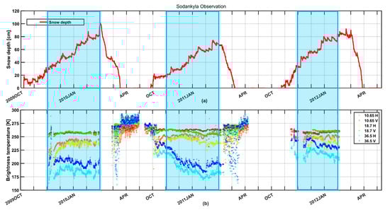
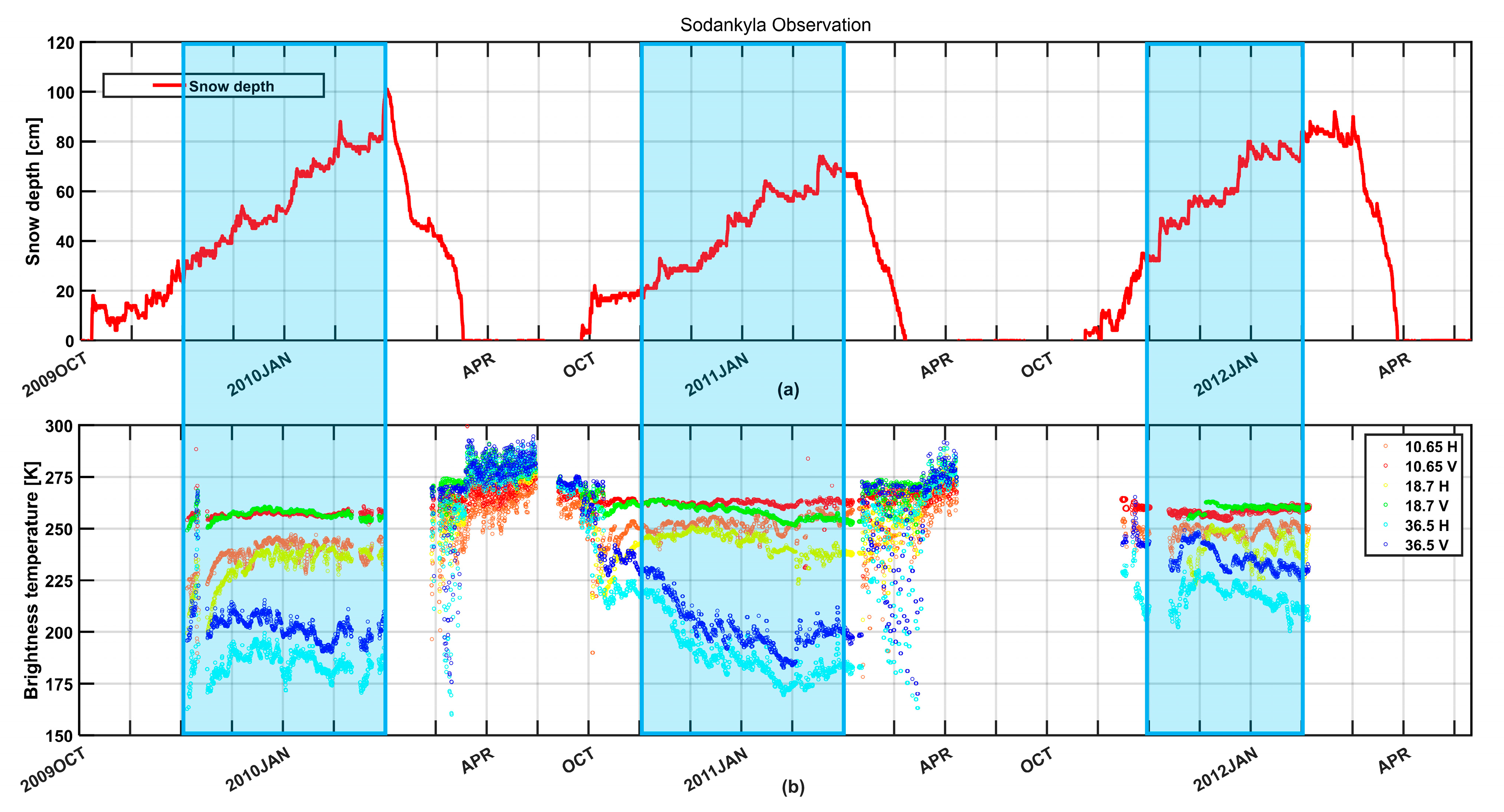
Figure 1.
The observed snow depth and passive microwave data in the NoSREx dataset. The blue-shaded areas are the dry snow periods studied in this experiment. (a) Snow depth (cm) from automated snow sensors in Sodankyla from 2009 to 2012. (b) The SodRad Tbs (K) with vertical and horizontal polarization at the X (10.65 GHz), Ku (18.7 GHz), and Ka (36.5 GHz) bands.
In this paper, the SodRad Tbs with observations every 3 h in 2009–2010 and every 4 h in 2010–2012 was used to test the retrieval framework. The observation angle was 50°. The six data channels taken included SodRad Tbs of the vertical and horizontal polarizations at 10.65, 18.7, and 36.5 GHz, which have been proven to reflect changes in snow cover in recent studies [32]. Figure 1 depicts the snow depth and SWE over three years, as well as the corresponding Tb measurements at the X, Ku, and Ka bands. The blue-shaded periods (mainly from 1 November to 31 March) represent the snow accumulation phases with dry snow as examined in this paper.
2.2. Proposed SWE Retrieval Framework
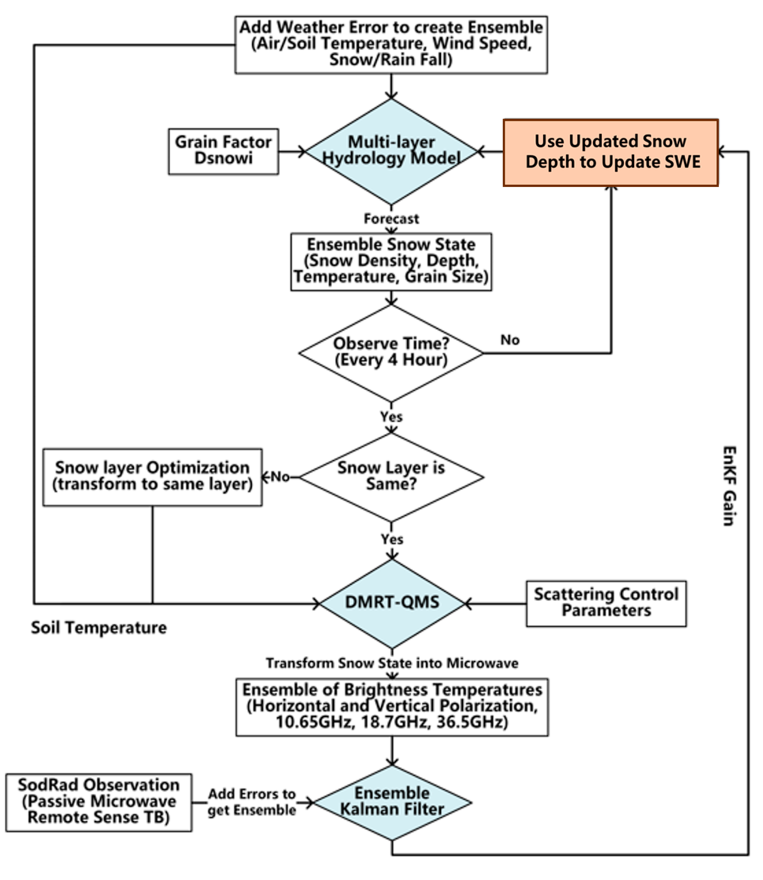
The framework of the coupled retrieval approach is illustrated in Figure 2. In this framework, every hydrological year (from November to May of the following year, hereafter, only the first three characters of the month (e.g., from NOV to MAY)) can be divided into three periods: the disturbance period, the assimilation period, and the snowmelt period. During the disturbance period, weather-driven variables (including snowfall, rainfall, wind speed, and air temperature) were perturbed before input into the snow hydrology model [35,36] to generate the initial ensembles of random snow states. The perturbations followed a normal distribution with zero means and the specified standard deviations listed in Table 1. The range of uncertainty was based on the NoSREx dataset. The number of ensembles was 100, which is determined in Section 3.3.3, to make the framework statistically efficient and accurate.

Figure 2.
The proposed SWE retrieval framework.

Table 1.
Weather forcing dataset error.
Next, these ensembles were used to drive the DMRT model [34] to simulate Tb ensembles at three frequency bands: 10.65 GHz, 18.7 GHz, and 36.5 GHz with both vertical and horizontal polarizations, for a total of six channels. Meanwhile, microwave remote sensing observations from these six channels were periodically introduced from the microwave radiometer observations into the DA system. The original observation interval for microwave observations was three or four hours. The number of observed Tb ensembles, generated from the NoSREx Tb standard deviation data, was 100, the same as the number of snow state ensembles. Finally, the forecasted snow depth ensembles from the hydrology model were improved by the radiometric measurements using the EnKF algorithm. The EnKF learned the linear relationship between the differences in snow depth and the differences in Tbs and applied this relationship to generate the posterior snow depth and Tb ensembles. Afterward, the updated snow depth ensembles from the EnKF were used as the initial conditions for the snow hydrology model in the next time step. With the update in snow depths, the other snow state ensembles, including the snow density, grain size, and temperature, would also be adjusted within the snow hydrology model in the next time step. The updated snow depth and adjusted snow density were used to adjust the SWE. The average values of the snow state ensembles were taken as final retrieval results at each time step.
2.2.1. Multilayer Snow Hydrology Model
This framework utilized the multilayer snow hydrology model developed by Kang et al. [35,36]. The model has several applications to demonstrate the year-round behavior of snowpack evolution [32,37]. Figure 3 shows a schematic view of a multilayered snowpack. The properties of each snow layer include the layer thickness (), snow temperature (), SWE, volumetric liquid water content (), bulk snow density (), and snow grain size (), which are also required inputs for the RT models. Heat and energy balance equations are used to evaluate the temperature and mass quantities (snow depth, density, and SWE) based on how the top layer interacts with the rest of the atmosphere.
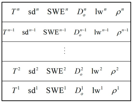
Figure 3.
Illustration of a multilayered snowpack. Notations are the IDs of different layers in bottom-first order.
The basic procedure for the adopted hydrology model is illustrated as follows. When snowfall or precipitation occurs below 0 , new snow accumulates on top of the uppermost layer of the snowpack. After the SWE reaches a threshold, the top layer is divided into two layers to retain a fine vertical resolution. By solving the energy balance equation as a function of the air temperature and heat conductivity of the top layer of snow, the temperature of the top snow layer is determined. Subsequently, the temperatures of the lower snow layers are governed by the heat conductivity of the snow medium and its interaction with the soil temperature. When the top layer’s snow temperature is above the melting point at 0, liquid water is released. When melting occurs, the mass balance equation allows the movement of liquid water from the top to the lower snow layers. For the snow microstructure, Jordan formulated the snow grain size using a grain growth function [39]. The derivative of the grain growth rate is defined as follows:
where is an adjustable grain growth factor, which is a hyperparameter, and is the mean snow grain size. To characterize the temporal dynamics of , its initial value, represented in Figure 2 as , is also needed. Changes in the snow grain growth factor and the initial grain size lead to variations in snow grain sizes and affect the microwave responses to a given multilayered snowpack [39].
The inputs of the hydrology model were the weather forcing data and the initial snow states at this time. Based on the mass and energy balances, the model calculated the snow state at the next time.
2.2.2. DMRT-QMS Model
DMRT-QMS [40,41,42] is a physical scattering model that is widely adopted for active and passive microwave modeling of snowpacks based on the dense media radiative transfer theory (DMRT) [34]. The DMRT theory predicts the microwave intensity scattering, absorption, and propagation in a dense random media. In DMRT-QCA, the approach of quasi-crystal approximation (QCA) [34] is applied to characterize snow scattering characteristics by solving the multiple scattering of densely packed sticky spheres with moderate grain sizes. The QCA approach provides a broad range of frequency-, size-, and density-dependent scattering characteristics with moderate forward scattering patterns. The size of the snow grains, the stickiness of the snow, the snow density or equivalently the ice volume fraction, and the temperature of the snow all affect these characteristics. In DMRT-QMS, the discrete ordinate method with eigenvalue analysis is used to solve the radiative transfer equation with multiple scattering effects among ice particles. DMRT-QMS computes both the Tbs and the backscattering coefficients of a snowpack. In this paper, the DMRT-QMS model was adopted to simulate the Tbs of the snowpack as synthesized by the snow hydrology model.
2.2.3. EnKF Algorithm
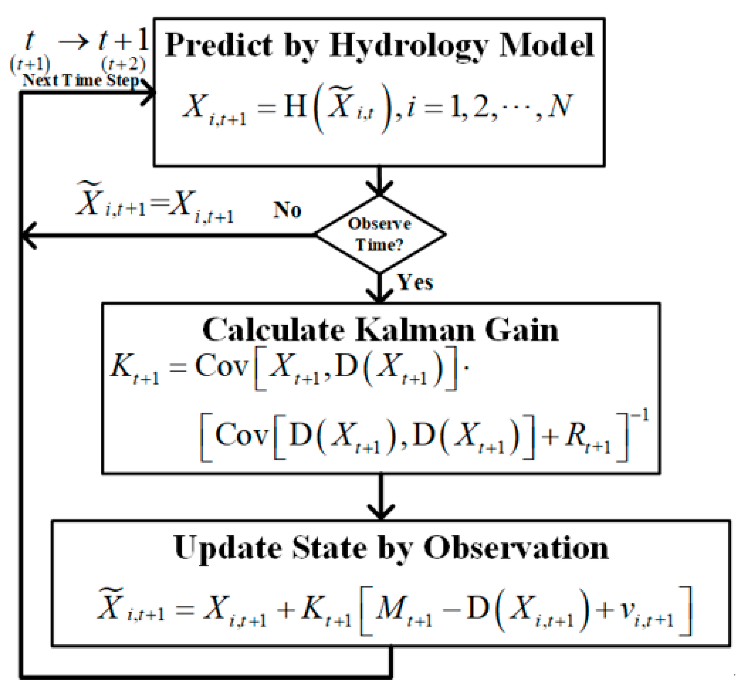
The EnKF [43,44,45,46] is an assimilation method that is widely used to fuse multi-source data in fields such as meteorology and hydrology [47,48]. The principle of the EnKF is to minimize the autocovariance matrix of the forecasted ensembles by coupling observations so that we can find the updated (i.e., posterior) ensembles [43,44,45,46]. This paper applies the EnKF algorithm to combine weather forcing data with microwave observations through a hydrology model in cascade with a RT model . The flowchart is illustrated in Figure 3.
As shown in Figure 4, in our framework, the snow state was first forecasted by the snow hydrology model as follows:
where each time step is 1 h. The th snow state ensemble forecasted by the snow hydrology model at this time step is represented by , and is a column vector, with a dimension of the total number of snow layers times the amount of snow depth to describe each layer. To maintain the physical constraints among multiple snow state variables, we opted to only update the snow depth of each layer in the EnKF algorithm. The other variables were automatically determined by the hydrology model following the updated snow depths. is the number of random samples in the ensemble. The larger is, the more accurate the result is, while leading to a longer calculation time. is the operator representing the snow hydrology model. is the snow state updated by the EnKF at time step . The update at this time step , as driven by microwave observations of the Tb, is illustrated as follows:
where is a vector that represents the microwave remote sensing observations at this time step , is the operator representing DMRT to convert the snowpack state into its corresponding microwave observations, and is the th observation error at this time step, which is assumed to be a Gaussian random variable with a standard deviation that characterizes the microwave sensor accuracy [38]. The Kalman gain at this time step is calculated as follows [46]:
where Rt+1 denotes the observation error covariance matrix. If microwave observations are not available at this time step, the EnKF correction is skipped until the next observation time. In the EnKF algorithm, the Kalman gain matrix is estimated as shown in Equation (4) from , the covariance matrix of the snow state ensembles and their corresponding Tb simulations, and , which is the autocovariance matrix of the simulated Tbs. Equations (5) and (6) provide estimations of the covariance matrices, and they converge as the ensemble size increases. This method is widely used to solve nonlinear numerical assimilation problems [43,44,45,46].
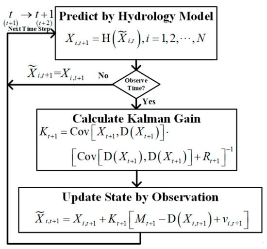
Figure 4.
The EnKF flow chart in the proposed framework.
2.2.4. Snow Layer Adjustment
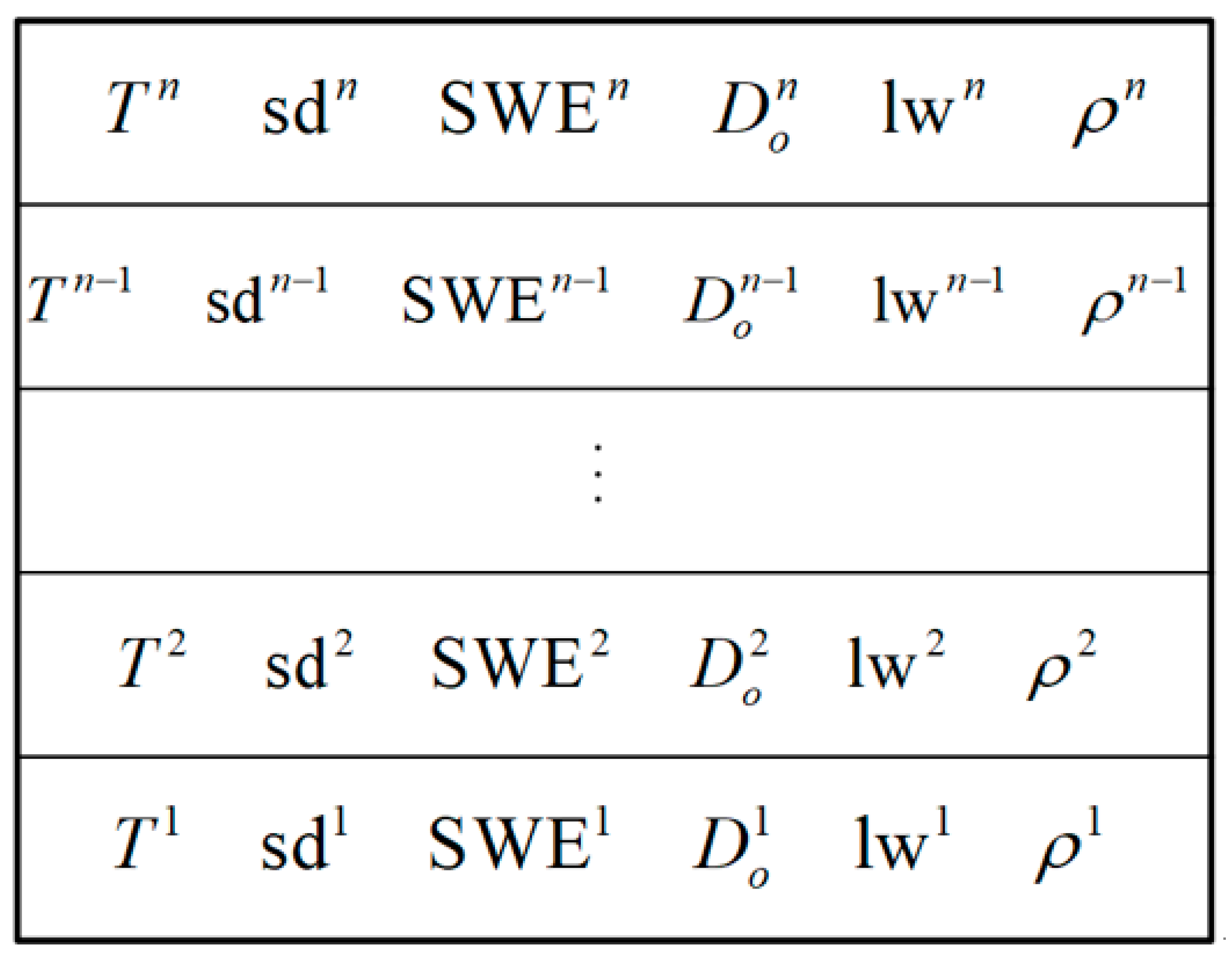
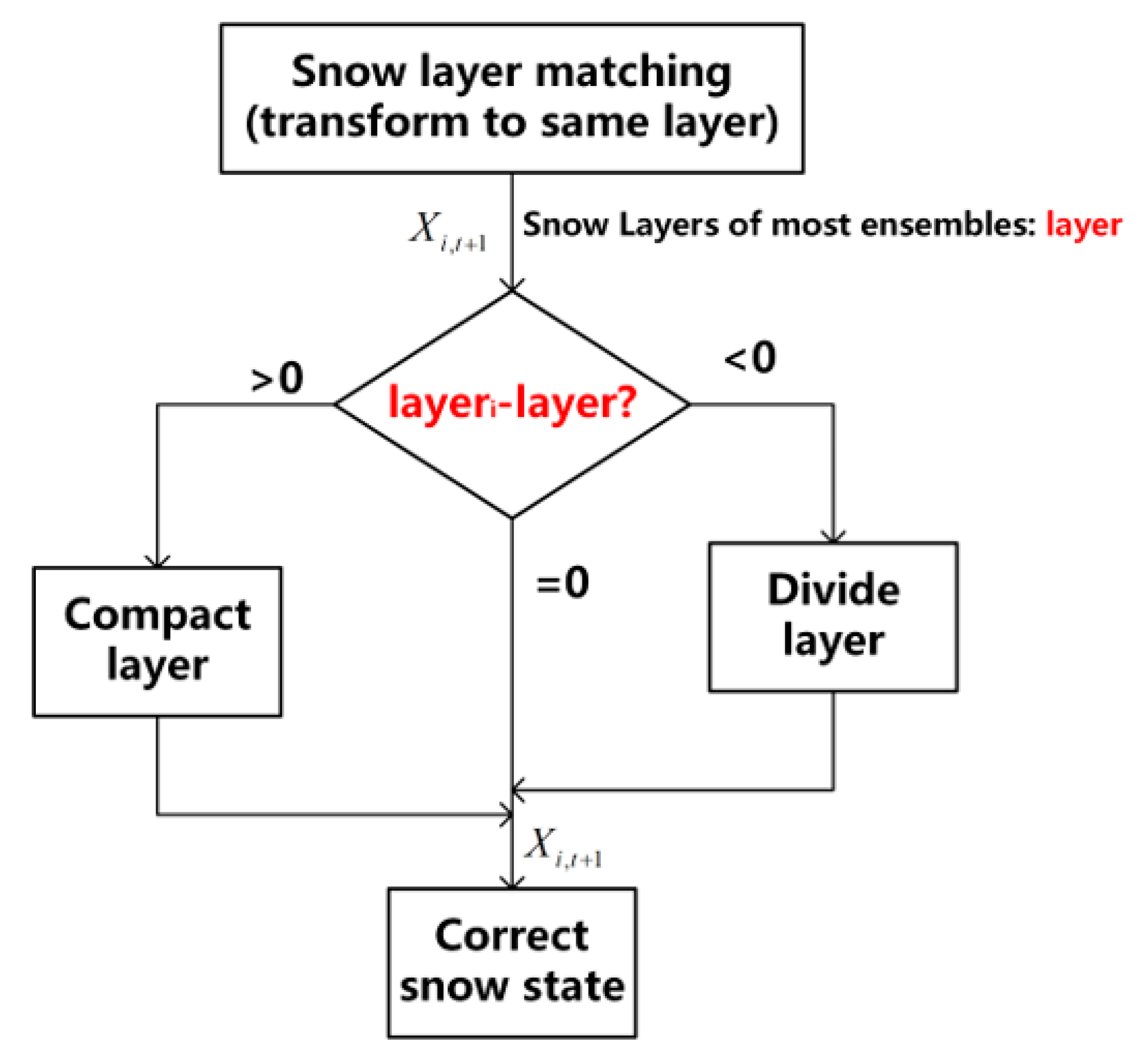
Since this framework uses a time-varying multilayer snow hydrology model, the introduction of disturbances may lead to inconsistencies in the number of snow layers between different ensembles at the same time point, which causes the matrix to have a dissatisfaction rank. While the calculation of the Kalman gains with Equation (4) requires matrix inversion, we propose an optimization to make the snow layers consistent in each ensemble. The idea of layer optimization is shown in Table 2 and Figure 5, which refer to the compact and divided snow layer logic of the snow hydrology model [35,36]. The top layer determines the number of layers of compacted or divided snow.
Table 2.
Optimization of snow ensemble layers.
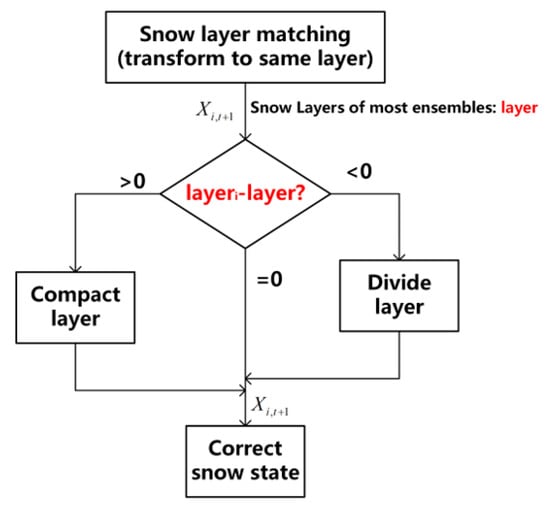
Figure 5.
Logic diagram for snow layer number optimization. The th layer is the number of snow layers for the th ensemble. The red ‘layer’ is the number of snow layers for the general ensemble, and layeri-layer means the layer from each ensemble minus the snow layer from most ensembles.
2.3. Selection of Undetermined Model Parameters
There are several remaining issues to be addressed to streamline the retrieval framework. First, the snow hydrology model has input parameters (e.g., the grain size parameters and ) which are not directly available from measurements. Second, the DMRT model requires more inputs than those provided by the hydrology model. For example, the snow/soil interface roughness parameters and the soil moisture are neither predicted by the hydrology model nor fully available from in situ observations. However, all of these parameters will affect the Tb predictions by the DMRT model, and we need a systematic approach to specify these parameters. This is converted into an optimization problem by tuning the hydrology model outputs to match the in-situ observations while minimizing the error between the DMRT-predicted Tbs and microwave observations [28].
Specifically, these undetermined parameters include the effective snow grain size, grain growth rate, and adjustment factor from the snow hydrology model, as well as the snow/soil interface roughness parameters and soil moisture volumetric fraction value from the DMRT-QMS model. First, we will establish appropriate ranges for these parameters using a combination of a literature review, empirical studies, and sensitivity analysis. To initiate the optimization process, the known parameters and initial values for undetermined parameters (e.g., grain size and growth rate) are fed into the framework. These initial values are chosen from within the established ranges for each undetermined parameter. The optimization algorithm will then iteratively adjust the parameters within their defined ranges by minimizing the root mean square error (RMSE) between the simulated Tbs from the DMRT-QMS model and the actual observed Tbs from the NoSREx dataset. In essence, this approach establishes a link between the undetermined parameters and the accuracy of the Tb simulation.
2.4. Evaluation of Porposed Framework
This section covers more detailed evaluation of the proposed framework. More comparisons are made regarding how changing the built-in parameters affects the assimilation results: the combination of observation frequencies, the time intervals between observations, and the number of ensembles. Also, in order to evaluate the feasibility of this framework, the assimilation results will be compared with the commonly used SWE retrieval algorithm.
3. Results
3.1. The Grain Size Scaling Factor and Internal Parameters of the Model
This framework was established such that the outputs of the snow hydrology model could drive the DMRT model, which converted the snow states obtained from the snow hydrology model into simulated Tbs so that they could be compared with the microwave observations. Among the key parameters that affect the Tb are the snow grain size , snow depth , and snow density . Inspired by earlier works [34,35,36], we adopted a linear factor to link the snow grain size predicted by the hydrology model to the snow grain size taken by the DMRT model :
This is to account for the fact that the hydrology model and the DMRT model assumed different conventions in defining the grain sizes. The coefficient is a parameter to be determined.
Aside from those standard variables, which the two models share, the other internal parameters of the two models are equally important. Among the input variables of the snow hydrology model are two control parameters: the snow grain factor and the initial snow grain size, which are called in Figure 3. These two factors are used to calculate the snow grain size for the snow hydrology model. The former is to control the growth rate of the grain size, and the latter is to set the initial snow grain size. The ranges of these two values were taken from previous works [35,36] and could update themselves at each time step. On the other hand, the DMRT-QMS model also has some internal hyperparameters for the surface roughness parameters and and soil moisture . For the snow/soil surface roughness parameters, we adopted a / model [34] to represent the effects of roughness on microwave emission, yielding another two free parameters, and , to be determined. The details of these parameters were presented in a previous work [32]. In this paper, the soil moisture is referenced to the average value shown in the NoSREx [38]. This value ought to vary with time, but we only took the more desirable average value from experience in this paper.
Figure 6a,d,g shows that the Tb decreased with increasing snow depths at each frequency band and was almost linear at 10.65 GHz and 18.7 GHz. While 36.5 GHz was more sensitive to light snow, which is less than 50 cm, the sensitivity decreased with increasing snow depths, which does not reflect the variation of deep snow. This is because when the snow is deeper (), the scattering effect of the snow saturates the high-frequency Tbs so that the information on the surface under the snow is not available. Meanwhile, different snow grain size scaling factors had a significant effect on the Tb. When , it was equivalent to directly substituting the snow grain size of the snow hydrology model into the DMRT model to obtain simulated Tbs. As decreased, the sensitivity of the Tb to the variation in snow depth at low frequencies decreased, and the sensitivity of deep snow at high frequencies increased, which was gradually consistent with the changes in the NoSREx data [38].
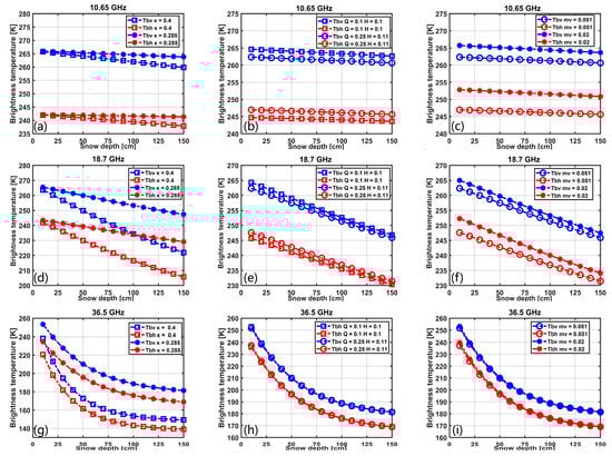
Figure 6.
Single-variable model parameter testing. (a,d,g) The effect of various snow grain size scaling parameters on the Tb. Tbs were simulated via DMRT-QMS at three bands, with both polarizations for different snow grain size scale factors with increasing snow depths. Fixed parameters: snow grain size , snow density , ground temperature , snow temperature , incidence angle , surface roughness , and soil moisture . (b,e,h) The effect of different roughness parameters on the Tb. Fixed parameters: , and the rest of the parameters are the same as above. (c,f,i) The effect of various soil moistures on the Tb. Fixed parameters: the same as above.
Figure 6b,c,e,f,h,i shows that the effects of the surface roughness (,) and soil moisture on the Tb decreased with increasing snow depths. Because of the deep snow, snow scattering accounted for most of the Tbs, weakening the effects of surface roughness on the Tbs. And we can see that the effect of these two parameters on the Tb at 36.5 GHz was negligible. These two parameters’ effect was only about at 10.65 GHz and 18.7 GHz, which is smaller compared with the effect of the scaling factor and is insensitive to the snow depth.
These experiments also showed that Tbs at different frequency bands could vary with the snow depth, and thus it is a reasonable choice to improve the snow depth estimation through microwave remote sensing of Tbs. Meanwhile, the scaling factor had a great influence on the Tb. It is significant to choose a suitable scaling factor so that the Tbs simulated by DMRT can be the same as the microwave observation Tbs when the forecasted snow depth from the hydrology model is the same as the observation of the snow depth. To determine this scaling factor , we chose the period at the beginning of the second year, when the snow depth forecasted by the snow hydrology model was generally the same as the observed snow depth. A suitable scaling factor was optimized when the Tbs simulated by DMRT closely matched the observed Tbs. It was appropriate to use this period to determine the best scaling factor and the other internal parameters for these two models, and these parameters would remain constant throughout the entire snow season. An example from the 2010–2011 snow year is shown in Figure 7.
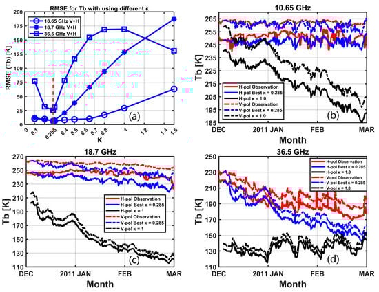
Figure 7.
Optimal hyperparameter experiment. (a) RMSE for Tbs using various values. (b) V-pol and H-pol of 10.65 GHz. (c) V-pol and H-pol of 18.7 GHz. (d) V-pol and H-pol of 36.5 GHz. The DMRT model simulated three frequencies (10.65, 18.7, and 36.5 GHz) compared with the observed Tbs. The blue line is the best match for the observations. Best parameters: scaling factor , surface roughness , and soil moisture .
Figure 7 illustrates the procedure to determine the grain size scaling factor in the retrieval framework. Figure 7a shows the RMSE of using the different scaling factor , which is the difference between the DMRT-simulated determination of these optimal parameters, the simulated Tbs, and the observed Tbs for each band. It can be seen that at the red dashed line, where , the RMSEs of all three bands was at its minimum value. When in the 10.65 GHz and 18.7 GHz bands, the RMSE increased when increased, while at 36.5 GHz, when , the RMSE decreased instead, which was different from the other two bands. Figure 7b–d shows the Tbs simulated by DMRT compared with the observed Tbs when choosing the best scaling factor and internal parameters. It shows that when no scaling factor () was used, there was a large gap between the simulated Tbs and the observed Tbs, during which the forecasted snow depth was the same as the observed snow depth. Therefore, it was necessary to use the scaling factor and to determine the internal parameters of the two models so that the simulated Tbs could correspond to the observed Tbs well. After several tests and comparisons, the best scaling factor and internal parameters were obtained (scaling factor , surface roughness and ). It can be seen that after determining these optimal parameters, the simulated Tbs coincided with the observed Tbs such that the snow depth could be improved using our framework through the microwave remote sensing observation of the Tb. Finally, the internal parameters of the snow hydrology model and DMRT are shown in Table 3.
Table 3.
The optimized internal parameters of the snow hydrology model and DMRT.
3.2. Assimilation Results for Snow Depth and SWE
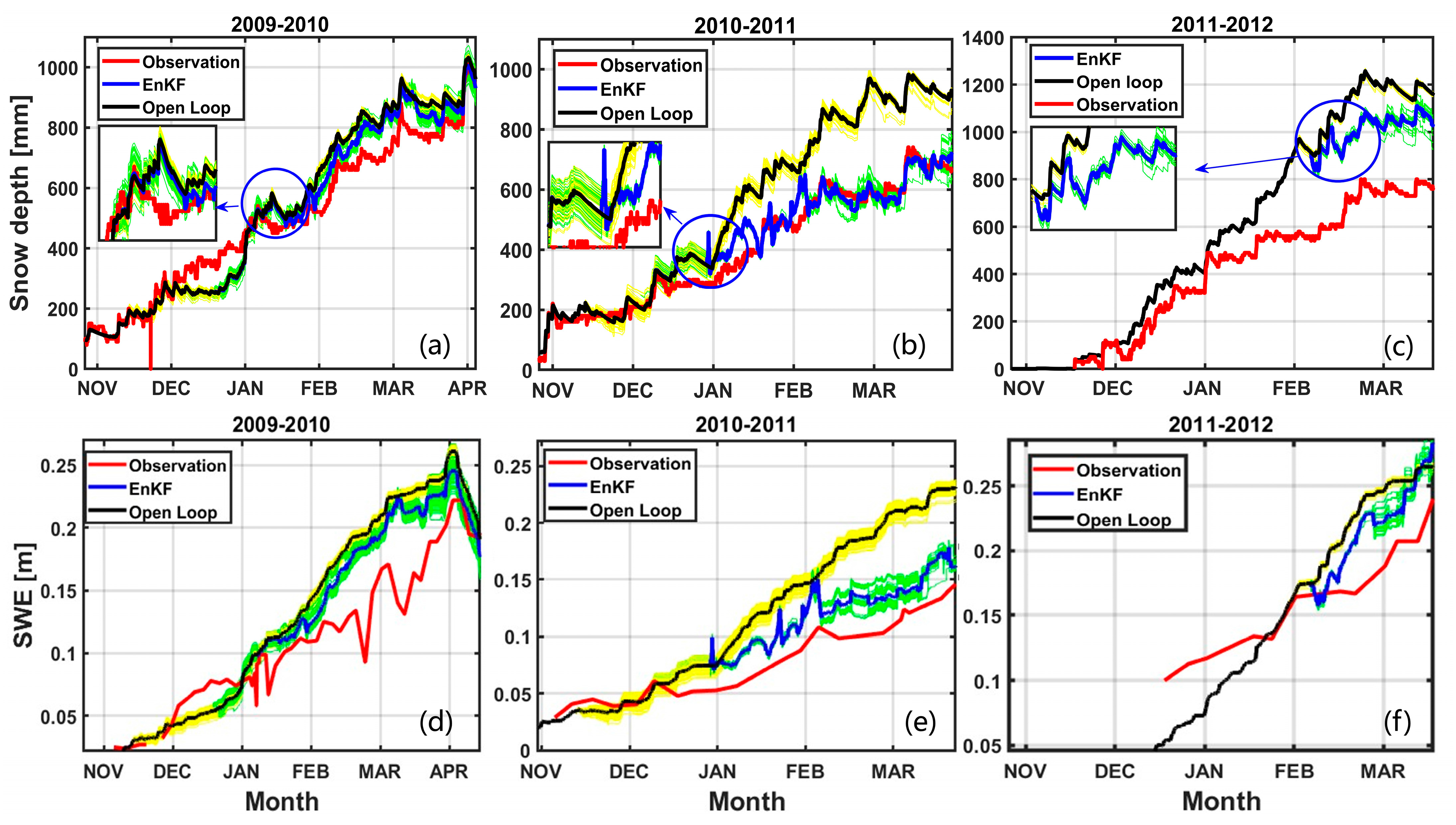
In this section, we conduct a comprehensive analysis of snow depth and SWE disparities across three key components: hydrologic model forecasts, framework enhancements, and actual observations. Employing an optimized model parameter and rigorous testing, the assimilation periods were strategically chosen based on meticulous considerations. During 2009–2011, the disturbance period predominantly spanned from November to December, with assimilation exclusively occurring between December and March. As the DMRT-QMS model cannot simulate wet snow, the snowmelt period from March to May was excluded from consideration during this time frame. From 2011 to 2012, the disturbance period shifted from November to February, constraining assimilation opportunities to the period from February to March. Therefore, the refined temporal alignment ensured that assimilation activities were synchronized with the relevant climatic conditions, enhancing the accuracy and applicability of the results.
Figure 8 presents the comparison of the best assimilation results for snow depth and SWE through the EnKF with the hydrologic model forecast and actual observation. It shows that the forecast ensemble range (yellow) was consistent with the range of the improved ensemble (green) during the disturbance period (NOV–DEC) and that this period was just preparation for the initial data of the framework in the next stage. During the assimilation period, each forecast ensemble was adjusted at the observed time points when microwave observation was available. In the period from 2009 to 2011, it is shown that the error range (green) of the improved posterior ensembles shrunk rapidly while the error range (yellow) of the forecasted prior ensembles was unchanged, which is shown in the details in the blue circle. This implies that the EnKF algorithm reduced the error range of the ensemble through microwave observation. During 2011–2012, the Tb observations were missing in the early period, which led to less information about the environment in the early snow season. The results were, therefore, worse compared with the first two years. It can be seen that the assimilated snow depth and SWE using the EnKF method were closer to the observations than the forecasted snow depth and SWE.
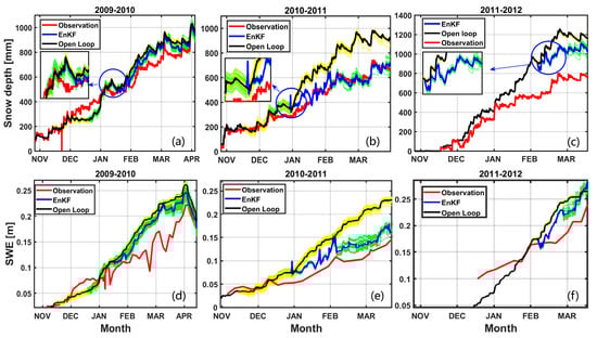
Figure 8.
Snow depth and SWE assimilation results (only in the snow accumulation period) in Sodankyla for the hydrological years during 2009–2012. (a,d) 2009–2010. (b,e) 2010–2011. (c,f) 2011–2012. The blue line shows the posterior ensembles’ mean after being improved by the EnKF and observations, and the green area is the range of the posterior ensembles. The black line shows the prior ensembles’ mean from the open-loop hydrology model, and the yellow area is the range of the prior ensembles. The red line shows the real observation. The small panel on the left side shows the details at the beginning of the assimilation circled in blue.
Table 4 shows the comparison statistics of the assimilated snow depth and SWE over the dry snow periods (JAN–APR) of three years. The following RMSEs were computed from the ensembles’ mean snow depth and SWE through the EnKF or open-loop model (blue line and black line, respectively, in Figure 8) with actual observations. All the RMSEs of the improved snow state decreased compared with the RMSEs of the open-loop snow hydrology model. During 2010–2011, the EnKF showed the RMSE of the snow depth decreasing to 28.12 mm and the SWE RMSE decreasing to 12.43 mm. Due to the most comprehensive microwave observations in this year with limited missing observations, it achieved the best performance. However, the results from 2011 to 2012 are not reliable because of the snow hydrology model forecast and extensive missing microwave data for this year. Overall, the SWE retrieval was better than the snow depth retrieval because the improved snow density was adaptively calculated by the hydrology model using the improved snow depth in the next time step. In these three years, the achieved SWE retrieval average RMSE was 34.31 mm, which meets the reference requirements of NASA SCLP and ESA CoReH2O [49,50], and it was about 70% lower than the open-loop snow hydrology model’s forecast error.
Table 4.
RMSE of snow depth and SWE compared with actual observations over dry snow periods (JAN–APR) of three years.
3.3. Evaluation of Proposed Framework
3.3.1. Combination of Different Observation Frequencies
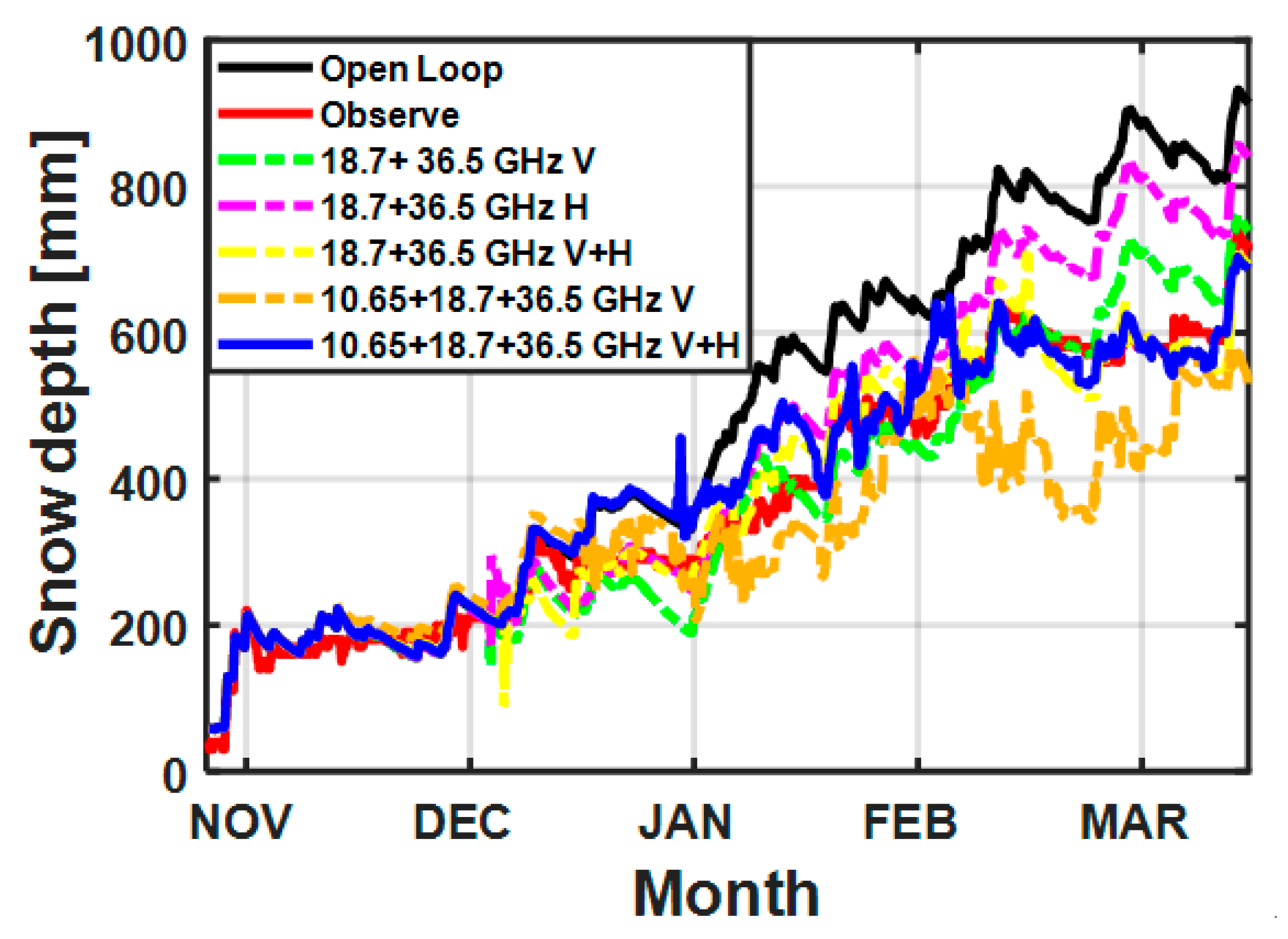
According to the analysis in Section 3.1, the sensitivity of different frequency bands corresponds to different snow depths. Previous studies also used different combinations of frequency bands, such as Chang’s work using a combination of 18.7 and 36.5 GHz V-pol to retrieve the SWE [8]. This section tests the effect of different polarization combinations at different frequency bands on the assimilated snow depth results in 2010–2011. Partially successful results are shown in Figure 9.
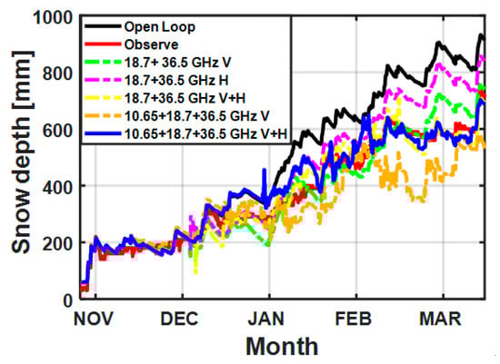
Figure 9.
The effect of different frequency band combinations on snow depth results during 2010–2011. V = V-pol; H = H-pol.
Figure 9 demonstrates that when using only 18.7 and 36.5 GHz, the retrieval of snow depth performed well in shallow snow but not in deep snow because the Ku (18.7 GHz) and Ka (36.5 GHz) bands were more sensitive to snow depth changes in the shallow snow case and less sensitive to snow depth changes in the deep snow case. This finding is consistent with the previous analysis in Section 3.1. In addition, V-pol reflects changes in snow depth more quickly than H-pol, which is why V-pol was mostly used in the previous works. To improve the low sensitivity of deep snow, we added the 10.65 GHz band (X band) to the combination because the band at 10.65 GHz had a similar linear trend to the change in snow depth. In Table 5, we also find that only using V-pol may have overestimated the change in snow depth, resulting in results lower than the observations. While H-pol may reflect some features that V-pol does not reflect, which can reduce noise, it can also make use of sensitivity to changes in snow density after new snowfall. Therefore, it was necessary to combine the respective characteristics of V-pol and H-pol to obtain the new observation combination (i.e., V-pol and H-pol at 10.65 + 18.7 + 36.5 GHz). The RMSEs of the above experiments were calculated as shown in Table 5. The results show that the RMSE of 28.12 mm was the lowest when using 10.65 + 18.7 + 36.5 GHz V-pol and H-pol. When other band combinations were used, the retrieval was not as good, but the retrieval results were improved compared with the open-loop forecast. This again shows that combining microwave observations can improve the snow depth forecast.
Table 5.
RMSEs of snow state compared with observations for different frequency combinations.
3.3.2. Observation Time Intervals
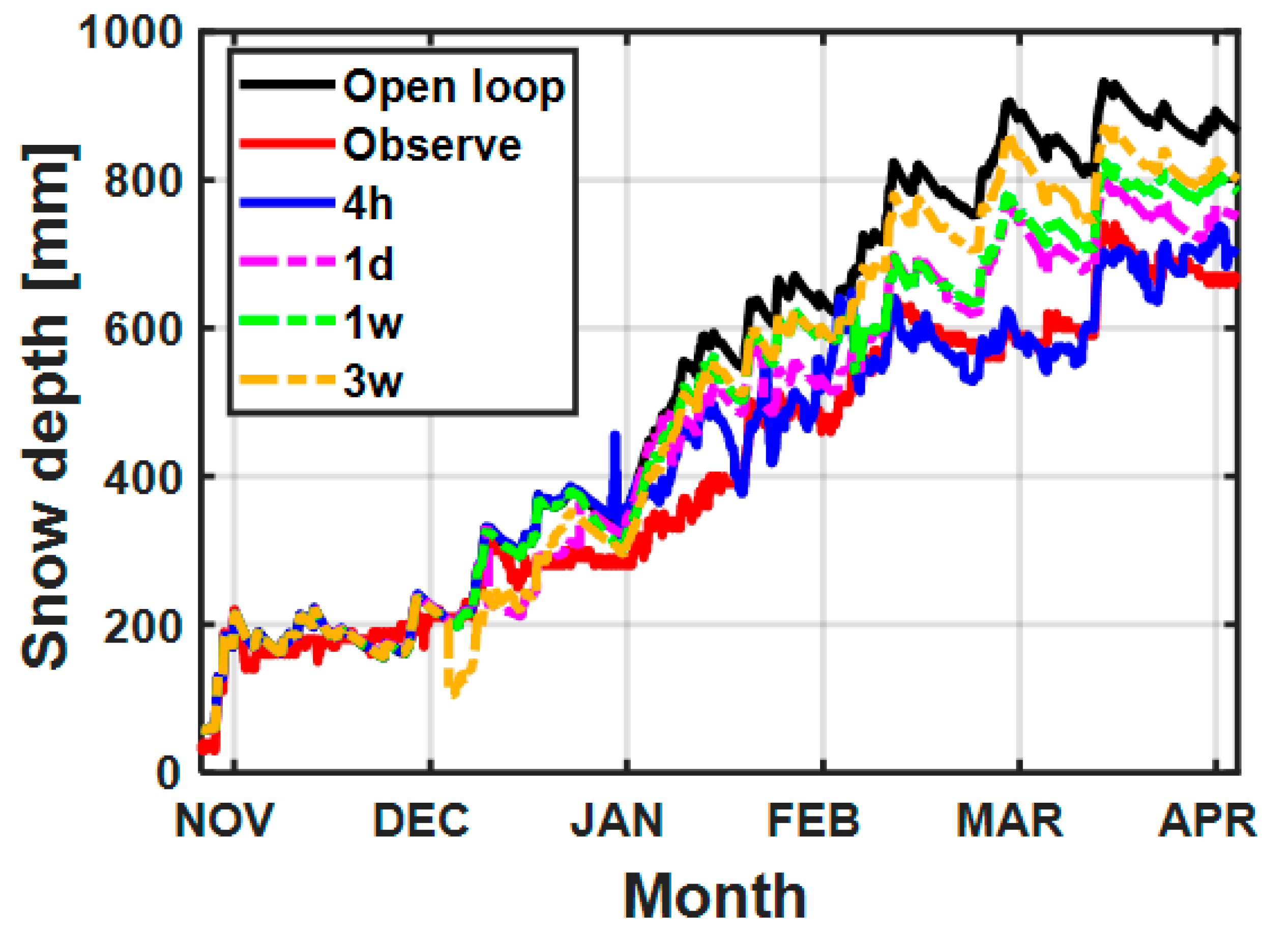
Garnaud et al. noted that the improvement in snow depth retrieval by the EnKF is sensitive to observation time intervals [51]. Common microwave observation by satellite does not have such short time intervals as the NoSREx ground-truth observations, and it is likely to observe an area only once every few days or even several weeks. It is necessary to discuss the effect of the observation time interval on the results in the framework. According to the principle of the EnKF algorithm, the revisit time may affect the effectiveness of the assimilation results. Shorter observation time intervals indicate that the EnKF combines microwave observations to update the snow depth more frequently. The short time interval directly affects the final assimilation results. This section shows experiments conducted to discuss the effect of the observation time interval on the results during 2010–2011. It thus discusses different time intervals from 4 h to 3 weeks and compares the differences among them, as shown in Figure 10.
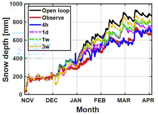
Figure 10.
The effect of different microwave observation time intervals on the results during 2010–2011. Legend: 4 h means every 4 hours, 1 d means every 1 day, and 1 w and 3 w mean every 1 week and 3 weeks, respectively.
Figure 10 shows that the assimilation results became worse as the observation time interval increased, which would result in the snow depth not being adjusted timely according to the microwave remote sensing observation. Meanwhile, a large time interval resulted in only the snow hydrology model dominating between two observation moments. As the time interval changed from 4 h to 3 weeks, the assimilation results approached the open-loop forecast. This implies that the information obtained from the microwave observations became weaker, and the forecast part of the snow hydrology model gradually became the dominant part. Table 6 shows the RMSEs for the four sets of time interval experiments. It implies that although the RMSEs increased with increasing observation time intervals, they were still improved and closer to the actual observations than the open-loop forecast using the hydrology model alone. Therefore, the framework can still optimize for snow states even at a larger observation time interval, which can be used for reality retrieval in the future. Moreover, the shorter the observation time interval chosen, the longer the calculation time, but the more accurately the assimilation was achieved.
Table 6.
RMSEs of snow state compared with different microwave observation intervals.
3.3.3. The Size of the Ensemble
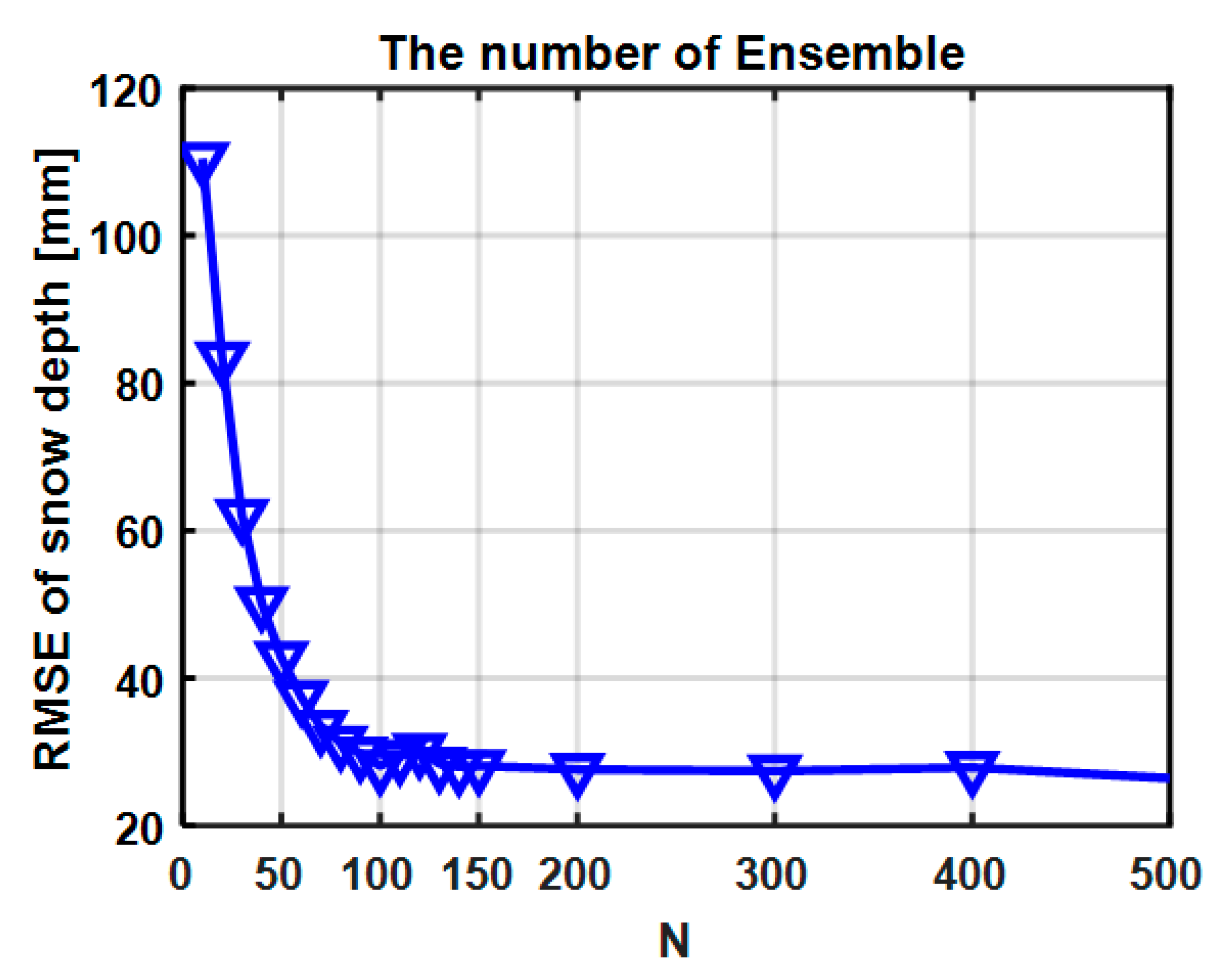
The number of ensembles in the EnKF affects the accuracy and computational efficiency of the assimilation results. Since the goal of the EnKF is to minimize the covariance matrix of the assimilation results, a larger value is desired to yield results closer to the real situation according to the central limit theorem (i.e., the principle of estimating the total from a sample). However, a larger value also affects computational efficiency, and thus there is a trade-off between efficiency and accuracy. This part discusses how the number of ensembles affects the RMSE of the final assimilation snow depth. Figure 11 shows that when was rather small, the RMSE of the snow depth estimation was larger, while when , the RMSE of the snow depth tended to be stable. When , the RMSE also decreased slightly, and the calculation became overburdened. Thus, from a computational efficiency perspective, the suitable number of ensembles in the framework we chose was .
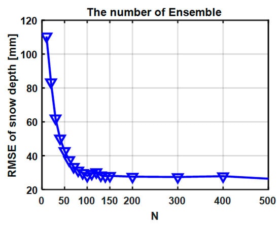
Figure 11.
The effect of different ensemble sizes on the RMSEs of snow depth estimation. The RMSEs were calculated between the posterior ensembles’ mean after being improved by the EnKF and actual observations.
3.3.4. Comparison of EnKF Approach with the Commonly Used SWE Retrieval Algorithm
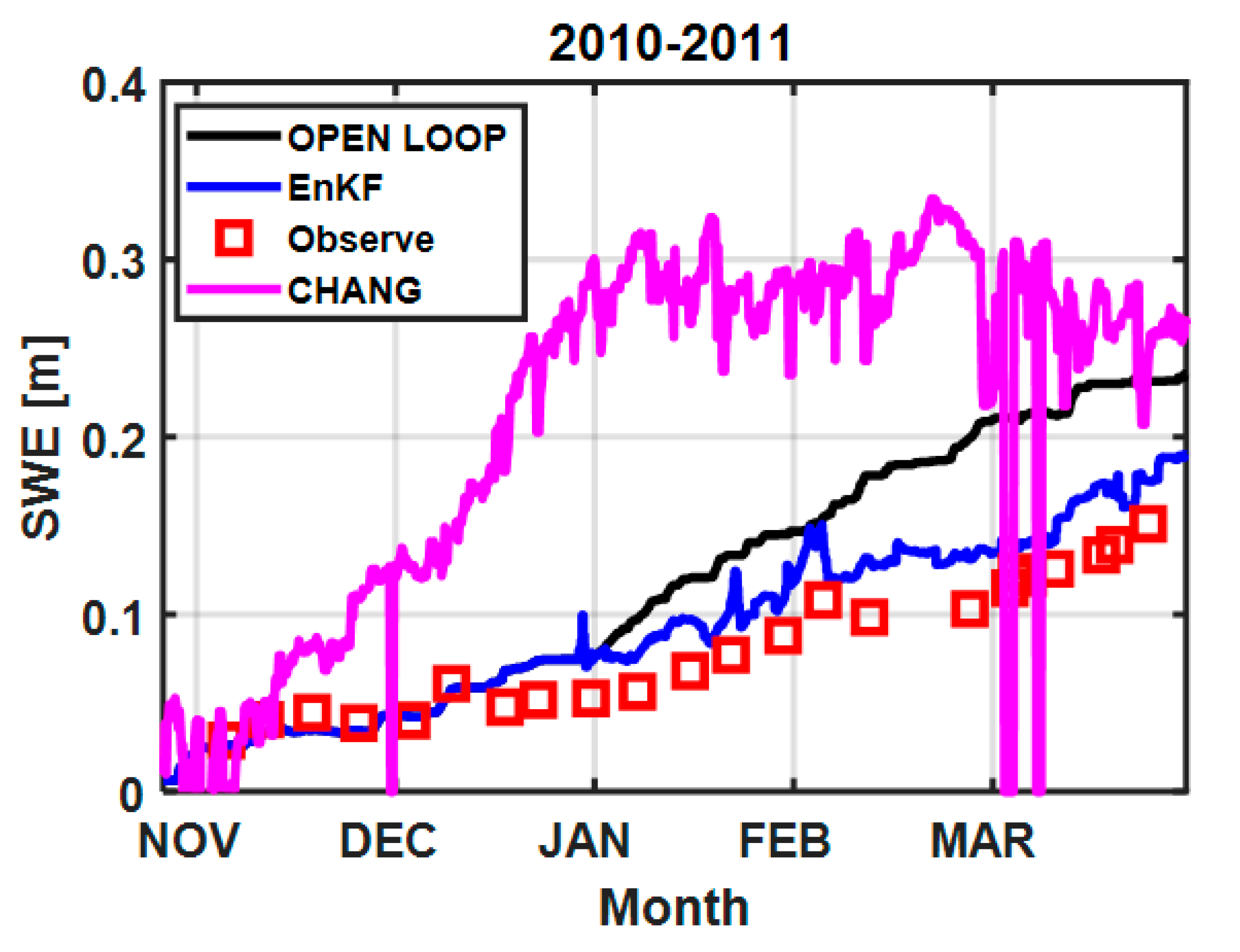
As the measurements for snow pits and microwave observations were intensive during 2010–2011, the SWE assimilation results from 2010–2011 were compared with Chang’s retrieval algorithm (Equation (9)), which has been widely used in global SWE retrieval [8]:
Figure 12 shows that Chang’s algorithm overestimated the SWE in the early snow accumulation season and underestimated the SWE in the late snow accumulation season due to lack of consideration of snow grain growth. This suggests the disadvantage of retrieving SWE through Tbs observations only. SWE from the proposed framework that combined the snow hydrology model with microwave observations matched better with the observation than the commonly used Chang’s algorithm.

Figure 12.
A comparison of SWE retrieval results from 2010 to 2011.
4. Discussion
4.1. Impact of Observation Quality on Snow Depth and SWE Retrieval over Three Years
The precision of the in situ and ground-based remote sensing observations utilized plays a crucial role in influencing the accuracy of the proposed framework’s retrieval of SWE. Specifically, it was expected that the passive microwave Ku and Ka bands would exhibit a more pronounced negative correlation with increasing snow depths in contrast to the X band. However, this relationship was primarily evident during the 2010–2011 period in the NoSREx. In the preceding year (2009–2010), while there existed a general negative correlation between the Ka and Ku bands and snow depth, the strength of this correlation was not as pronounced as that observed in 2010–2011. This is potentially linked to the year-to-year variations in snow grain size likely contributing to the varying sensitivity of the microwave observations of snow depths. In the work by Kang et al. [32], the evolution of the snow grain size in the snow seasons (as reported in Figure 6 of the paper) indicated that the winter of 2009–2010 in general had smaller grain sizes than those in the winter of 2010–2011. Thus, the volume scattering in the years 2009–2010 was weaker, leading to reduced correlation between the brightness temperatures and snow depths. It is also imperative to acknowledge that issues with the Tb measuring device were reported between 2011 and 2012, introducing potential errors and uncertainties into the collected Tb data [28]. Consequently, the variability in Tb observations across different bands became unstable during this period, raising concerns about potential data contamination.
The EnKF algorithm updates the modeled snow depth from the Kalman gain and the differences between the modeled and observed Tbs. The covariance of the modeled Tbs and snow depth is one of the key components in computing the Kalman gain. Thus, the accuracy of snow depth and SWE retrieval using the EnKF method relies on the accuracy of the Tbs observations and the actual relationship between the Tbs and snow depths. In 2010–2011, the observed Tbs and snow depths showed similar negative correlations (Figure 1) to the modeled correlation (Figure 6), resulting in good retrieval results for the snow depth. In contrast, the relationships between the observed Tbs and snow depths were not obvious in 2009–2010 or 2011–2012, resulting in limited improvement in the snow depth retrieval results in these two years.
Further examinations are needed when generalizing the approach to handling satellite observations. Satellite observations entail more complexities that are not present in ground measurements, including a coarse resolution, intricate terrain features, forest cover, atmospheric attenuation at high frequencies, frozen ground conditions, and mixed pixels [28,52,53]. Testing the performance of the proposed approach in such scenarios is needed, with potential improvements in the modeling capability and observation channel diversity.
4.2. The Impact of the Assimilated Snow Depth on Tb Predictions
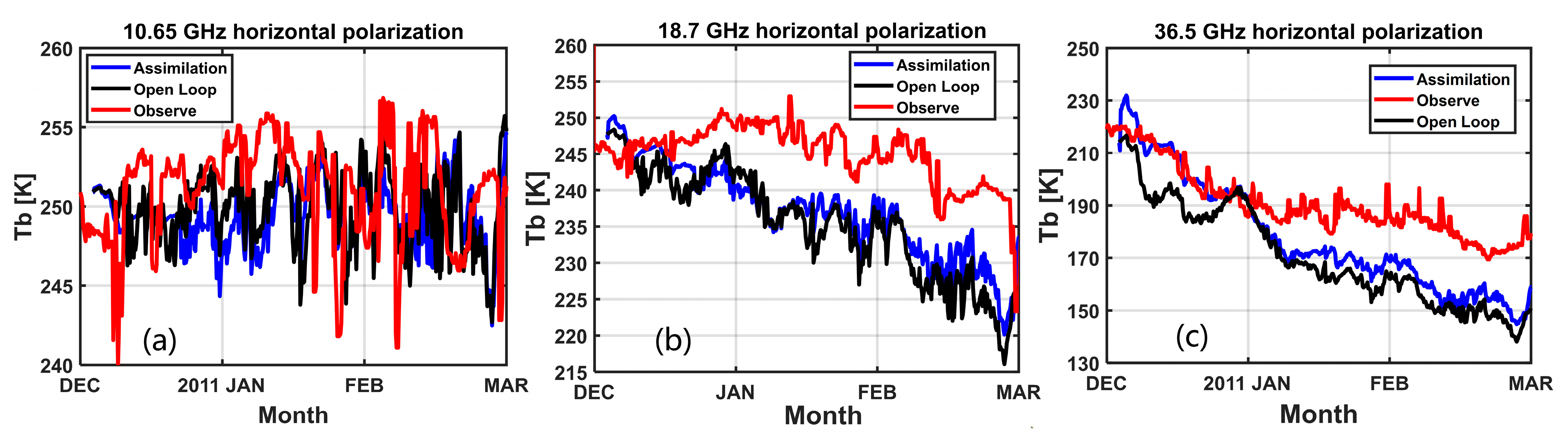
To assess the extent to which an updated snow depth improved the Tbs’ simulation, the Tbs were updated by running the DMRT model using the assimilated snow depth. Figure 13 displays a comparison of the horizontal polarization brightness temperatures (Tbs) for 2010–2011. Given the similarity of the changes between vertical polarization and horizontal polarization, we present analysis solely for the horizontal polarization. The updated Tbs represent Tbs computed from the updated snow depth. Notably, the updated Tbs (depicted by the blue line) exhibited a slightly closer alignment with the observed values (indicated by the red line) when compared with the open-loop Tbs (illustrated by the black line). However, it is worth noting that the improvement at 10.65 GHz was negligible. This was attributed to the lower sensitivity of the X band (10.65 GHz) to variations in snow depth when κ = 0.285, aligning with the diminished sensitivity of the observed values, as demonstrated in Figure 6 (Left column). In contrast, the Tbs at both 18.7 GHz (Ku) and 36.5 GHz (Ka) exhibited improvements over time, with 36.5 GHz showing a better enhancement. Nevertheless, a notable disparity persisted between the observed and simulated Tbs. While the model can provide a reasonable approximation of the relationship between Tbs and variations in snow depth, imperfect model accuracy may introduce errors in the reconstructed snow cover parameters. Further, the snow depth is not the sole snow property that the Tb is sensitive to. The snow grain size and density may have more impact on the Tb response during snow accumulation.
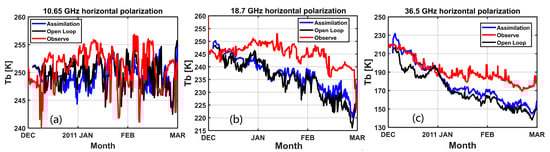
Figure 13.
Forecasted Tbs by hydrology model and posterior Tb (improved by EnKF) in 2010–2011 compared with observed Tbs. (a) H-pol. at 10.65 GHz, (b) 18.7 GHz, and (c) 36.5 GHz. The black line is the forecast Tbs, which is DMRT simulating through the average of the ensembles of the forecast snow states. The blue line is the posterior Tbs, which is from the average of the DMRT simulations using the posterior ensembles of the snow states. The red line is the observed Tbs.
The snow hydrology model parameters can potentially impact the accuracy of snow retrievals. Kang et al. [28] performed separate calibrations of the snow hydrology model for each year in the ESA NoSREx dataset to account for variations in snow properties. These dataset-specific calibrations might lead to overfitting and limit generalizability of the data assimilation framework. For real applications, the dataset to calibrate the snow hydrology model each year might not be available. Thus, the calibrated parameters in 2011 were used for the snow hydrology model over all three years in this paper. It is worth noting that fixed parameters within the DMRT model and the lack of year-specific calibration for these snow hydrology model parameters could impact the framework performance across different years, allowing us to examine the sensitivity of the DA framework to model parameter tuning.
5. Conclusions
This paper presented a retrieval framework that adopted the DA algorithm and the EnKF to improve the accuracy of SWE estimation by combining the 1D multilayer snow hydrology model and the passive microwave forward model (one of the available RT models: DMRT-QMS). The framework can reduce the RMSE in the SWE predicted by the hydrology model. The principle of the framework is to take into consideration the variation of forecast ensembles and the variation of observation ensembles to minimize the variance of the final assimilation ensembles, which leads to an optimal estimation combining all the information at each observation time. We used the ESA NoSREx dataset to verify the performance of the framework. The assimilation results showed that the achieved SWE retrieval RMSE averaged over the three years was 34.31 mm, which exceeded the reference requirements of the NASA SCLP and ESA CoReH2O missions and was about 70% lower than the open-loop snow hydrology model’s forecast. In general, this paper presented a novel framework for retrieving SWE that leverages the combined strengths of a snow hydrology model and a radiative transfer model. This approach ensures physically realistic snowpack properties throughout the retrieval process. We further investigated the impact of several factors on the framework’s performance, including the observation time intervals, combinations of microwave observation channels, and size of the ensemble. A few detailed findings of these applications are summarized as follows:
- The relationship of the snow grain size between the snow hydrology model and the DMRT model can be established by a scaling factor . In this framework, the established parameter was from the ESA NoSREx dataset analysis. In this study, a constant soil moisture and surface roughness parameters were assumed.
- The framework presented more flexibility in choosing the appropriate passive microwave observation channel combinations. The six channel observations (V- and H-pol at 10.65 GHz, 18.7 GHz, and 36.5 GHz), when applied together, worked better than other combinations for SWE retrieval.
- Different observation time intervals affected the assimilation results, and the longer the time interval, the more the assimilation results were biased toward the open-loop forecast values. In our test, the framework performed well for observation intervals less than seven days.
- The presented 1D framework can be extended to a wide spatial domain using a large spatial coverage of experimental data (for example, Environment Canada data [54] and NASA data [55]), where a distributed snow hydrology model is required [56,57]. Moreover, a more advanced RT model such as the DMRT-bicontinuous media model [58] can be adopted in the framework to improve the retrieval accuracy of SWE. The framework can also improve the performance of SWE retrieval for future applications that use both active and passive microwave observations.
Author Contributions
Conceptualization, S.T.; methodology, Y.C. and C.L.; results, Y.C. and C.L.; discussion, Y.C. and Y.F.; data curation, Y.C. and C.L.; writing—original draft preparation, Y.C., C.L., and Y.F.; visualization, Y.C. and C.L.; supervision, S.T.; manuscript revision: Y.C., Y.F., J.P. and D.-H.K.; Y.C. and C.L. contributed equally to this work. D.-H.K. provided the dataset and hydrology model scripts. All authors have read and agreed to the published version of the manuscript.
Funding
This work was supported by the National Key Research and Development Program of China under grant 2022YFB3903300 and grant 2022YFB3903303. It was also supported by the startup funds from Zhejiang University. Dr. Do-Hyuk Kang is partially supported by the Korea Environment Industry and Technology Institute through the Water Management Research Program, funded by the Korea Ministry of Environment (grant number: 79622). Dr. Jinmei Pan is partially supported by the Strategic Priority Research Program of the Chinese Academy of Sciences (grant number XDA20100300). This work was led by Principal Supervisor Dr. Shurun Tan.
Data Availability Statement
The NoSREx (-I -II and -III) dataset can be accessed through https://earth.esa.int/eogateway/campaigns/nosrex-i-ii-and-iii (accessed on 8 November 2023). Further details are available from the corresponding author upon reasonable request.
Conflicts of Interest
The authors declare no conflicts of interest.
References
- Sturm, M.; Goldstein, M.A.; Parr, C. Water and Life from Snow: A Trillion Dollar Science Question. Water Resour. Res. 2017, 53, 3534–3544. [Google Scholar] [CrossRef]
- Tsai, Y.-L.S.; Dietz, A.; Oppelt, N.; Kuenzer, C. Remote Sensing of Snow Cover Using Spaceborne SAR: A Review. Remote Sens. 2019, 11, 1456. [Google Scholar] [CrossRef]
- Barnett, T.P.; Adam, J.C.; Lettenmaier, D.P. Potential Impacts of a Warming Climate on Water Availability in Snow-Dominated Regions. Nature 2005, 438, 303–309. [Google Scholar] [CrossRef]
- Pomeroy, J.; de Boer, D.; Martz, L.W. Hydrology and Water Resources of Saskatchewan; Centre for Hydrology, University Saskatchewan: Saskatoon, Saskatchewan, 2005. [Google Scholar]
- Déry, S.J.; Stahl, K.; Moore, R.D.; Whitfield, P.H.; Menounos, B.; Burford, J.E. Detection of Runoff Timing Changes in Pluvial, Nival, and Glacial Rivers of Western Canada. Water Resour. Res. 2009, 45. [Google Scholar] [CrossRef]
- Kim, E.; Gatebe, C.; Hall, D.; Newlin, J.; Misakonis, A.; Elder, K.; Marshall, H.P.; Hiemstra, C.; Brucker, L.; De Marco, E. NASA’s SnowEx Campaign: Observing Seasonal Snow in a Forested Environment. In Proceedings of the 2017 IEEE International Geoscience and Remote Sensing Symposium (IGARSS), Fort Worth, TX, USA, 23–28 July 2017; IEEE: Piscataway, NJ, USA, 2017; pp. 1388–1390. [Google Scholar]
- Armstrong, R.L.; Chang, A.; Rango, A.; Josberger, E. Snow Depths and Grain-Size Relationships with Relevance for Passive Microwave Studies. Ann. Glaciol. 1993, 17, 171–176. [Google Scholar] [CrossRef]
- Chang, A.T.; Foster, J.L.; Hall, D.K. Nimbus-7 SMMR Derived Global Snow Cover Parameters. Ann. Glaciol. 1987, 9, 39–44. [Google Scholar] [CrossRef]
- Pulliainen, J.T.; Grandell, J.; Hallikainen, M.T. Retrieval of Surface Temperature in Boreal Forest Zone from SSM/I Data. IEEE Trans. Geosci. Remote Sens. 1997, 35, 1188–1200. [Google Scholar] [CrossRef]
- Pulliainen, J.T.; Grandell, J.; Hallikainen, M.T. HUT Snow Emission Model and Its Applicability to Snow Water Equivalent Retrieval. IEEE Trans. Geosci. Remote Sens. 1999, 37, 1378–1390. [Google Scholar] [CrossRef]
- Luojus, K.; Pulliainen, J.; Takala, M.; Lemmetyinen, J.; Mortimer, C.; Derksen, C.; Mudryk, L.; Moisander, M.; Hiltunen, M.; Smolander, T. GlobSnow v3. 0 Northern Hemisphere Snow Water Equivalent Dataset. Sci. Data 2021, 8, 163. [Google Scholar] [CrossRef]
- Pan, J.; Durand, M.T.; Vander Jagt, B.J.; Liu, D. Application of a Markov Chain Monte Carlo Algorithm for Snow Water Equivalent Retrieval from Passive Microwave Measurements. Remote Sens. Environ. 2017, 192, 150–165. [Google Scholar] [CrossRef]
- Saberi, N.; Kelly, R.; Pan, J.; Durand, M.; Goh, J.; Scott, K.A. The Use of a Monte Carlo Markov Chain Method for Snow-Depth Retrievals: A Case Study Based on Airborne Microwave Observations and Emission Modeling Experiments of Tundra Snow. IEEE Trans. Geosci. Remote Sens. 2020, 59, 1876–1889. [Google Scholar] [CrossRef]
- Xue, Y.; Forman, B.A. Comparison of Passive Microwave Brightness Temperature Prediction Sensitivities over Snow-Covered Land in North America Using Machine Learning Algorithms and the Advanced Microwave Scanning Radiometer. Remote Sens. Environ. 2015, 170, 153–165. [Google Scholar] [CrossRef]
- Forman, B.A.; Xue, Y. Machine Learning Predictions of Passive Microwave Brightness Temperature over Snow-Covered Land Using the Special Sensor Microwave Imager (SSM/I). Phys. Geogr. 2017, 38, 176–196. [Google Scholar] [CrossRef]
- Ahmad, J.A.; Forman, B.A.; Kwon, Y. Analyzing Machine Learning Predictions of Passive Microwave Brightness Temperature Spectral Difference over Snow-Covered Terrain in High Mountain Asia. Front. Earth Sci. 2019, 7, 212. [Google Scholar] [CrossRef]
- Cui, Y.; Xiong, C.; Lemmetyinen, J.; Shi, J.; Jiang, L.; Peng, B.; Li, H.; Zhao, T.; Ji, D.; Hu, T. Estimating Snow Water Equivalent with Backscattering at X and Ku Band Based on Absorption Loss. Remote Sens. 2016, 8, 505. [Google Scholar] [CrossRef]
- Oveisgharan, S.; Esteban-Fernandez, D.; Waliser, D.; Friedl, R.; Nghiem, S.; Zeng, X. Evaluating the Preconditions of Two Remote Sensing Swe Retrieval Algorithms over the Us. Remote Sens. 2020, 12, 2021. [Google Scholar] [CrossRef]
- Lawrence, D.M.; Fisher, R.A.; Koven, C.D.; Oleson, K.W.; Swenson, S.C.; Bonan, G.; Collier, N.; Ghimire, B.; van Kampenhout, L.; Kennedy, D. The Community Land Model Version 5: Description of New Features, Benchmarking, and Impact of Forcing Uncertainty. J. Adv. Model. Earth Syst. 2019, 11, 4245–4287. [Google Scholar] [CrossRef]
- Liang, X.; Wood, E.F.; Lettenmaier, D.P. Surface Soil Moisture Parameterization of the VIC-2L Model: Evaluation and Modification. Glob. Planet. Change 1996, 13, 195–206. [Google Scholar] [CrossRef]
- Niu, G.-Y.; Yang, Z.-L.; Mitchell, K.E.; Chen, F.; Ek, M.B.; Barlage, M.; Kumar, A.; Manning, K.; Niyogi, D.; Rosero, E. The Community Noah Land Surface Model with Multiparameterization Options (Noah-MP): 1. Model Description and Evaluation with Local-scale Measurements. J. Geophys. Res. Atmos. 2011, 116. [Google Scholar] [CrossRef]
- Andreadis, K.M.; Lettenmaier, D.P. Assimilating Remotely Sensed Snow Observations into a Macroscale Hydrology Model. Adv. Water Resour. 2006, 29, 872–886. [Google Scholar] [CrossRef]
- Andreadis, K.M.; Lettenmaier, D.P. Implications of Representing Snowpack Stratigraphy for the Assimilation of Passive Microwave Satellite Observations. J. Hydrometeorol. 2012, 13, 1493–1506. [Google Scholar] [CrossRef]
- Slater, A.G.; Clark, M.P. Snow Data Assimilation via an Ensemble Kalman Filter. J. Hydrometeorol. 2006, 7, 478–493. [Google Scholar] [CrossRef]
- Sun, C.; Walker, J.P.; Houser, P.R. A Methodology for Snow Data Assimilation in a Land Surface Model. J. Geophys. Res. Atmos. 2004, 109. [Google Scholar] [CrossRef]
- Durand, M.; Molotch, N.P.; Margulis, S.A. A Bayesian Approach to Snow Water Equivalent Reconstruction. J. Geophys. Res. Atmos. 2008, 113. [Google Scholar] [CrossRef]
- Durand, M.; Kim, E.J.; Margulis, S.A. Radiance Assimilation Shows Promise for Snowpack Characterization. Geophys. Res. Lett. 2009, 36. [Google Scholar] [CrossRef]
- Che, T.; Li, X.; Jin, R.; Huang, C. Assimilating Passive Microwave Remote Sensing Data into a Land Surface Model to Improve the Estimation of Snow Depth. Remote Sens. Environ. 2014, 143, 54–63. [Google Scholar] [CrossRef]
- Durand, M.; Kim, E.J.; Margulis, S.A.; Molotch, N.P. A First-Order Characterization of Errors from Neglecting Stratigraphy in Forward and Inverse Passive Microwave Modeling of Snow. IEEE Geosci. Remote Sens. Lett. 2011, 8, 730–734. [Google Scholar] [CrossRef]
- Kim, R.S.; Kumar, S.; Vuyovich, C.; Houser, P.; Lundquist, J.; Mudryk, L.; Durand, M.; Barros, A.; Kim, E.J.; Forman, B.A. Snow Ensemble Uncertainty Project (SEUP): Quantification of Snow Water Equivalent Uncertainty across North America via Ensemble Land Surface Modeling. Cryosphere 2021, 15, 771–791. [Google Scholar] [CrossRef]
- Huang, C.; Newman, A.J.; Clark, M.P.; Wood, A.W.; Zheng, X. Evaluation of Snow Data Assimilation Using the Ensemble Kalman Filter for Seasonal Streamflow Prediction in the Western United States. Hydrol. Earth Syst. Sci. 2017, 21, 635–650. [Google Scholar] [CrossRef]
- Kang, D.H.; Tan, S.; Kim, E.J. Evaluation of Brightness Temperature Sensitivity to Snowpack Physical Properties Using Coupled Snow Physics and Microwave Radiative Transfer Models. IEEE Trans. Geosci. Remote Sens. 2019, 57, 10241–10251. [Google Scholar] [CrossRef]
- Luo, C.; Tan, S.; Kang, D.-H. A Snow Water Equivalent Retrieval Framework Coupling Microwave Remote Sensing and Hydrology Model. In Proceedings of the 2021 IEEE International Geoscience and Remote Sensing Symposium IGARSS, Brussels, Belgium, 11–16 July 2021; IEEE: Piscataway, NJ, USA, 2021; pp. 7256–7259. [Google Scholar]
- Tsang, L.; Chen, C.-T.; Chang, A.T.; Guo, J.; Ding, K.-H. Dense Media Radiative Transfer Theory Based on Quasicrystalline Approximation with Applications to Passive Microwave Remote Sensing of Snow. Radio Sci. 2000, 35, 731–749. [Google Scholar] [CrossRef]
- Kang, D.H.; Barros, A.P. Observing System Simulation of Snow Microwave Emissions over Data Sparse Regions—Part I: Single Layer Physics. IEEE Trans. Geosci. Remote Sens. 2011, 50, 1785–1805. [Google Scholar] [CrossRef]
- Kang, D.H.; Barros, A.P. Observing System Simulation of Snow Microwave Emissions over Data Sparse Regions—Part II: Multilayer Physics. IEEE Trans. Geosci. Remote Sens. 2011, 50, 1806–1820. [Google Scholar] [CrossRef]
- Kang, D.H.; Barros, A.P.; Dery, S.J. Evaluating Passive Microwave Radiometry for the Dynamical Transition from Dry to Wet Snowpacks. IEEE Trans. Geosci. Remote Sens. 2013, 52, 3–15. [Google Scholar] [CrossRef]
- Lemmetyinen, J.; Kontu, A.; Pulliainen, J.; Vehviläinen, J.; Rautiainen, K.; Wiesmann, A.; Mätzler, C.; Werner, C.; Rott, H.; Nagler, T. Nordic Snow Radar Experiment. Geosci. Instrum. Methods Data Syst. 2016, 5, 403–415. [Google Scholar] [CrossRef]
- Jordan, R.E. A One-Dimensional Temperature Model for a Snow Cover: Technical Documentation for SNTHERM. 89. 1991; pp. 5. Available online: https://erdc-library.erdc.dren.mil/jspui/handle/11681/11677 (accessed on 15 November 2023).
- Tsang, L.; Pan, J.; Liang, D.; Li, Z.; Cline, D.W.; Tan, Y. Modeling Active Microwave Remote Sensing of Snow Using Dense Media Radiative Transfer (DMRT) Theory with Multiple-Scattering Effects. IEEE Trans. Geosci. Remote Sens. 2007, 45, 990–1004. [Google Scholar] [CrossRef]
- Liang, D.; Xu, X.; Tsang, L.; Andreadis, K.M.; Josberger, E.G. The Effects of Layers in Dry Snow on Its Passive Microwave Emissions Using Dense Media Radiative Transfer Theory Based on the Quasicrystalline Approximation (QCA/DMRT). IEEE Trans. Geosci. Remote Sens. 2008, 46, 3663–3671. [Google Scholar] [CrossRef]
- Chang, W.; Tan, S.; Lemmetyinen, J.; Tsang, L.; Xu, X.; Yueh, S.H. Dense Media Radiative Transfer Applied to SnowScat and SnowSAR. IEEE J. Sel. Top. Appl. Earth Obs. Remote Sens. 2014, 7, 3811–3825. [Google Scholar] [CrossRef]
- Evensen, G. The Ensemble Kalman Filter: Theoretical Formulation and Practical Implementation. Ocean. Dyn. 2003, 53, 343–367. [Google Scholar] [CrossRef]
- Evensen, G. Data Assimilation: The Ensemble Kalman Filter; Springer: Berlin/Heidelberg, Germany, 2009; ISBN 978-3-642-03710-8. [Google Scholar]
- Burgers, G.; van Leeuwen, P.J.; Evensen, G. Analysis Scheme in the Ensemble Kalman Filter. Mon. Weather. Rev. 1998, 126, 1719–1724. [Google Scholar] [CrossRef]
- Houtekamer, P.L.; Mitchell, H.L. Data Assimilation Using an Ensemble Kalman Filter Technique. Mon. Wea. Rev. 1998, 126, 796–811. [Google Scholar] [CrossRef]
- Pan, M.; Wood, E.F. Data Assimilation for Estimating the Terrestrial Water Budget Using a Constrained Ensemble Kalman Filter. J. Hydrometeorol. 2006, 7, 534–547. [Google Scholar] [CrossRef]
- Zhang, H.; Hendricks Franssen, H.-J.; Han, X.; Vrugt, J.A.; Vereecken, H. State and Parameter Estimation of Two Land Surface Models Using the Ensemble Kalman Filter and the Particle Filter. Hydrol. Earth Syst. Sci. 2017, 21, 4927–4958. [Google Scholar] [CrossRef]
- Elder, K.; Cline, D.; Liston, G.E.; Armstrong, R. NASA Cold Land Processes Experiment (CLPX 2002/03): Field Measurements of Snowpack Properties and Soil Moisture. J. Hydrometeorol. 2009, 10, 320–329. [Google Scholar] [CrossRef]
- Rott, H.; Duguay, C.; Essery, R.; Haas, C.; Macelloni, G.; Malnes, E. ESA SP-1313/3 Candidate Earth Explorer Core Missions Report for Assessment: CoReH20—Cold Regions Hydrology High Resolution Observatory. ESA Commun. Prod. Off. 2009. [Google Scholar]
- Garnaud, C.; Bélair, S.; Carrera, M.L.; Derksen, C.; Bilodeau, B.; Abrahamowicz, M.; Gauthier, N.; Vionnet, V. Quantifying Snow Mass Mission Concept Trade-Offs Using an Observing System Simulation Experiment. J. Hydrometeorol. 2019, 20, 155–173. [Google Scholar] [CrossRef]
- Xiao, X.; He, T.; Liang, S.; Zhao, T. Improving Fractional Snow Cover Retrieval From Passive Microwave Data Using a Radiative Transfer Model and Machine Learning Method. IEEE Trans. Geosci. Remote Sens. 2022, 60, 1–15. [Google Scholar] [CrossRef]
- Zschenderlein, L.; Luojus, K.; Takala, M.; Venäläinen, P.; Pulliainen, J. Evaluation of passive microwave dry snow detection algorithms and application to SWE retrieval during seasonal snow accumulation. Remote Sens. Environ. 2023, 288, 113476. [Google Scholar] [CrossRef]
- Carrera, M.L.; Bélair, S.; Bilodeau, B. The Canadian Land Data Assimilation System (CaLDAS): Description and Synthetic Evaluation Study. J. Hydrometeorol. 2015, 16, 1293–1314. [Google Scholar] [CrossRef]
- Kwon, Y.; Forman, B.A.; Ahmad, J.A.; Kumar, S.V.; Yoon, Y. Exploring the Utility of Machine Learning-Based Passive Microwave Brightness Temperature Data Assimilation over Terrestrial Snow in High Mountain Asia. Remote Sens. 2019, 11, 2265. [Google Scholar] [CrossRef]
- Girotto, M.; Musselman, K.N.; Essery, R.L.H. Data Assimilation Improves Estimates of Climate-Sensitive Seasonal Snow. Curr. Clim. Chang. Rep. 2020, 6, 81–94. [Google Scholar] [CrossRef]
- Lehning, M.; Völksch, I.; Gustafsson, D.; Nguyen, T.A.; Stähli, M.; Zappa, M. ALPINE3D: A Detailed Model of Mountain Surface Processes and Its Application to Snow Hydrology. Hydrol. Process. 2006, 20, 2111–2128. [Google Scholar] [CrossRef]
- Tan, S.; Chang, W.; Tsang, L.; Lemmetyinen, J.; Proksch, M. Modeling Both Active and Passive Microwave Remote Sensing of Snow Using Dense Media Radiative Transfer (DMRT) Theory With Multiple Scattering and Backscattering Enhancement. IEEE J. Sel. Top. Appl. Earth Obs. Remote Sens. 2015, 8, 4418–4430. [Google Scholar] [CrossRef]


Disclaimer/Publisher’s Note: The statements, opinions and data contained in all publications are solely those of the individual author(s) and contributor(s) and not of MDPI and/or the editor(s). MDPI and/or the editor(s) disclaim responsibility for any injury to people or property resulting from any ideas, methods, instructions or products referred to in the content. |
© 2024 by the authors. Licensee MDPI, Basel, Switzerland. This article is an open access article distributed under the terms and conditions of the Creative Commons Attribution (CC BY) license (https://creativecommons.org/licenses/by/4.0/).