Abstract
The remove–compute–restore (RCR) approach is widely used in local quasi-geoid modeling. However, the classical RCR approach usually does not take into account the noise of the satellite-only global gravity field model (GGM), which may lead to a suboptimal result. This paper presents an approach for local quasi-geoid modeling based on spherical radial basis functions that combines local noisy datasets and a noisy satellite-only GGM. This approach includes an RCR procedure using a satellite-only GGM. This is a direct approach that takes the spherical harmonic coefficients of satellite-only GGM as a noisy dataset and includes the corresponding full-noise covariance matrix in the least-squares estimation, aiming to obtain a statistically optimal local quasi-geoid model. The direct approach goes beyond the indirect approach, which treats the height anomalies generated from the satellite-only GGM as a noisy dataset. However, the generated GGM height anomaly dataset is not an equivalent representation of the satellite-only GGM, which may result in the loss of information from the satellite-only GGM. Through mathematical deduction, we demonstrate the theoretical consistency between the direct approach and the indirect approach. The direct approach also has an advantage over the indirect approach in terms of computational complexity due to the simpler algorithm. We conducted a synthetic closed-loop test with a real data distribution in Colorado, and numerical results demonstrated the advantage of the direct approach in local quasi-geoid modeling. In terms of the root mean square of the differences between the predicted values and the true reference values, the direct approach provided an improvement of approximately 14% compared to the indirect approach.
1. Introduction
Exploring high-precision methods for local quasi-geoid modeling is of great significance for the realization of the International Height Reference System (IHRS) [1]. This is because the disturbing potential values at reference stations need to be determined using the appropriate quasi-geoid modeling method, which is crucial for calculating the geopotential numbers of the IHRS reference stations [2].
Over the past two decades, the Gravity Recovery and Climate Experiment (GRACE) and GRACE Follow-On missions and the Gravity Field and Steady-State Ocean Circulation Explorer (GOCE) mission have collected a large amount of satellite-to-satellite tracking (SST) data and gravity gradient data, respectively. Based on these satellite data, many satellite-only global gravity field models (GGMs) have been established, providing the middle- to long-wavelength signal of the Earth’s gravity field. Moreover, with the use of post-fit residual analysis [3], an effective tool for analyzing the noise model of satellite data, the latest satellite-only GGMs are equipped with reliable full-noise covariance matrices (NCMs), such as GOCO05s [4] and GOCO06s [5]. To this day, the remove–compute–restore (RCR) approach [6] is still frequently used in local quasi-geoid modeling. However, the classical RCR approach does not use the satellite-only GGM in the same way as local datasets such as terrestrial and airborne data, thereby neglecting the noise in the satellite-only GGM, which may result in a suboptimal model [7].
Based on the theory of the geodetic boundary-value problems, commonly used methods for local quasi-geoid modeling can be summarized as three types: Stokes/Molodensky integral and its various modified formulas, least-squares collocation (LSC), and the spherical radial basis function (SRBF) method [8,9,10]. In theory, for all three types of methods, some publications have already considered the combination of local datasets with a noisy GGM in the RCR procedure. The spectral combination approach [11,12,13] includes the modified Stokes kernel and employs the error degree variances of the GGM, but generally does not employ the full NCM of the GGM. The recently proposed residual LSC (RLSC) approach [14,15] is an improvement upon the standard LSC approach, and the modified formula of LSC includes the full NCM of the GGM. Compared to covariance matrices derived from error degree variances or empirical covariance fitting, using an anisotropic and location-dependent full NCM in local quasi-geoid modeling facilitates realistic error model estimation. In this paper, we focus on the combination of local datasets with a noisy GGM in the SRBF method.
SRBFs have good localization properties, and it is easy to combine heterogeneous datasets using SRBFs. Therefore, SRBFs are a powerful tool for local quasi-geoid modeling. In particular, when using least-squares techniques to estimate the SRBF model, it is possible to include the NCMs of the datasets and provide the NCM of the estimated parameters, which is of significant importance for uncertainty analysis of the geopotential numbers at the IHRS reference stations. For the SRBF method, there are currently two statistically optimal ways to combine local datasets and a noisy satellite-only GGM (or satellite datasets): (1) directly using the original satellite datasets along with their NCMs [16]; (2) using the height anomalies computed on the Earth’s surface via spherical harmonic (SH) synthesis from the satellite-only GGM, with the corresponding NCM propagated from the NCM of the satellite-only GGM’s SH coefficients [7,17,18]. In the first approach, the complex functional model and the huge amount of data tend to constrain the use of low-low and high-low SST data. The second approach (referred to as the “indirect approach” for brevity) has been recently proposed. The indirect approach first computes the height anomalies using a satellite-only GGM at pre-defined grid points on the Earth’s surface, treating them as a low-resolution GGM dataset. Then, by combining the GGM dataset and the high-resolution local datasets, a two-scale SRBF model is established. There are two main problems with the indirect approach: (1) the generated GGM height anomaly dataset is not an equivalent representation of the satellite-only GGM, making this conversion non-lossless; (2) it is necessary to sufficiently expand the local data area to compute the coarse-scale model, whereas, in practice, it cannot be guaranteed that the neighboring area of the target area has available high-resolution datasets. Moreover, the NCM of the GGM height anomaly dataset is extremely ill-conditioned, increasing the difficulty of parameter estimation [17].
In this study, we propose a direct approach for combining local datasets and a noisy satellite-only GGM. In the direct approach, the SH coefficients of the satellite-only GGM and their full NCM are directly treated as a noisy dataset. Compared to the first two approaches, the direct approach is simpler and more efficient. This is because SRBFs are constructed based on SHs, and there exists a close theoretical connection between them [19]. Moreover, the SRBF coefficients and SH coefficients have an explicit analytical relationship [20]. To the best of our knowledge, no publication has studied the direct approach. One important reason may be that the analytical relationship between the SRBF coefficients and the SH coefficients relies on the orthogonality of the surface SHs over the unit sphere. If the target area is on a global scale, the direct approach can certainly be adopted. However, can the direct approach still be adopted if the target area is on a local scale? Furthermore, what is the connection between the direct approach and the indirect approach? This paper aims to address the two research questions.
This paper is organized as follows. In Section 2, we present the direct approach and revisit the indirect approach, demonstrating their theoretical consistency. In Section 3, we conduct a synthetic closed-loop test. In Section 4, we analyze and discuss the experimental results. Finally, we provide the conclusion and give the outlook in Section 5.
2. Methodology
2.1. SHs and SRBFs
Let x be a three-dimensional coordinate vector of any point outside the sphere with reference radius R, and denotes the normalized vector of x. The disturbing potential of point x has the following approximate SH expansion:
where GM denotes the product of the gravitational constant and mass of the Earth, and L denotes the maximum SH degree. and denote the 4π fully normalized SH coefficients and the surface SH of degree l and order m, respectively. We can rewrite Equation (1) as
wherein
Let z be a three-dimensional coordinate vector of a point on the sphere with radius r, uniformly covering the whole sphere , and the sphere is completely enclosed by the topographic masses. The disturbing potential at any point x outside the sphere can be approximated by a series expansion of the SRBFs:
where denotes the SRBF coefficient. SRBF is defined as
where and denote the Legendre coefficient and the Legendre polynomial of degree l, respectively. Based on the orthogonality relations of the surface SHs on the unit sphere, the following SHs addition theorem holds [21]:
Substituting Equations (6) and (7) into Equation (5) yields the following equation:
which can be rewritten as
wherein
Define as a vector, and
Due to the orthogonality of surface SHs on the unit sphere, the integral over the sphere of the product of and is a unit matrix, namely
where denotes the surface element of the sphere . Now, calculate the integral of the product of and over the sphere :
Substituting Equation (2) into Equation (16) yields the following equation:
where is a diagonal matrix, and
Substituting Equation (9) into Equation (16) yields the following equation:
where diagonal matrix , and
By comparing Equation (17) and Equation (19), the analytical relationship between the SH coefficients and the SRBF coefficients can be obtained:
wherein
is a matrix. If the SRBF coefficients are known, Equation (21) can be used to determine the SH coefficients. It should be noted that in this case, I should be larger than , i.e., the number of SRBFs is “admissible” [19].
2.2. Direct Approach
Since Equation (21) relies on the orthogonality of surface SHs on the unit sphere, the SRBF model should be considered at a global scale. However, in local modeling, SRBFs are constrained within the local parameterization area of the sphere , and the SRBFs outside the area are ignored, which is equivalent to setting the SRBF coefficients outside the area to zero [22]. By merging the zero coefficients and the coefficients inside the area , the overall SRBF model is defined on the whole sphere . In the synthesis step, zero coefficients automatically vanish, therefore no additional setup is required in practice. The SRBF coefficient vectors inside and outside the area are denoted as and , respectively, where is a zero vector. Thus, we have
where k is the number of SRBFs inside the area . Substituting Equation (23) into Equation (5), Equation (21) is replaced by
wherein
In fact, Equation (24) has been used in previous studies. For example, Wittwer [23] employed Equation (24) to analyze the noise spectrum of the terrestrial dataset and compared it with the noise spectrum from the satellite-only GGM dataset, demonstrating the improvement of GRACE data for the local gravity field model; Bucha et al. [22] used Equation (24) to convert band-limited SRBF coefficients into SH coefficients (also known as the correction signal) and added the correction signal to the original GGM, resulting in an SH model specifically tailored for the Slovak Republic. However, Equation (24) is used in reverse in the direct approach, i.e., the SH coefficients are used to estimate the SRBF coefficients. When using the RCR approach, the modeling object is the residual disturbing potential, as the middle- to long-wavelength signal provided by the satellite-only GGM is removed from the disturbing potential. It is also for this reason that, in the direct approach, the mathematical expectations of the residual SH coefficients of the residual disturbing potential are zero within the corresponding spectral band. Thus, the following functional model can be obtained:
where denotes the residual SH coefficient vector, denotes the expectation operator, and denotes the dispersion operator. The NCM of the residual SH coefficient vector is none other than the NCM of the SH coefficients of the satellite-only GGM. By combining Equation (26) and the functional models of the local datasets, the overall linear Gauss–Markov model is obtained for estimating the SRBF coefficients.
2.3. Indirect Approach
In the indirect approach, the satellite-only GGM is first used to compute the height anomalies at pre-defined grid points on the Earth’s surface. According to Bruns’ formula [21], the height anomaly is defined as
where denotes the normal gravity of point x on the telluroid. According to Equation (2), the height anomaly computed using the satellite-only GGM can be expressed as
Based on Equation (9), the following observation equation can be established:
Obviously, Equation (29) implicitly includes a constraint condition that sets the vector of the SRBF coefficients outside the area to a zero vector, i.e., .
Calculating the integral of the product of and over the sphere based on Equation (17) and Equation (19), respectively, we have
For any , Equation (30) holds. Since Equation (24) can also be derived from Equation (30), the direct approach and the indirect approach are theoretically equivalent. However, the computational procedure of the indirect approach is complex.
3. Experiment Settings
To validate the performance of the direct approach, we conducted a simulation experiment with Colorado (USA) as the core area and compared the results with the classical RCR approach and the indirect approach. The reason for conducting the simulation experiment is that noise-free control data are advantageous for interpreting the results.
3.1. Datasets
The study area (also referred to as the data area) belongs to the Rocky Mountains, and it is bound by 100.8°W to 111.2°W and 33.8°N to 41.2°N. The rugged terrain increases the difficulty of the quasi-geoid modeling. We use the high-resolution EIGEN-6C4 [24] model complete to degree 2190 to generate gravity disturbance data and add white Gaussian noise with a standard deviation (STD) of 1 mGal to simulate the local dataset. Due to the knowledge of the actual terrestrial dataset within the area between 102°W and 110°W and 35°N and 40°N, the 20,000 data points within this area simulate the distribution of the actual dataset [2]. Furthermore, there are an additional 9000 data points randomly distributed in other areas of the study area. Figure 1 illustrates the topography of the study area as well as the distribution of data points.
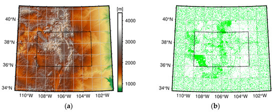
Figure 1.
(a) The topography of the study area and the target area (black rectangle); (b) the distribution of the local data points.
3.2. Classical RCR Approach
To better understand this section, please first read Appendix A to learn about the two-scale SRBF model used in the indirect approach. This is because the single-scale model shown in Equation (A5) is the model established using the classical RCR approach. Therefore, the main task of the classical RCR approach is the estimation of the coefficient set .
RCR procedure. To reduce the errors of linearization and spherical approximation, we removed the GOCO05s model complete to degree 280 and the XGM2016 [25] model from degree 281 to 719 from the local gravity disturbance data. In mountainous areas, topographic effects also play an important role [22,26], so we further removed the topographic model dV_ELL_Earth2014 [27] from degree 720 to 2190 from the local gravity disturbance data. After the GGM reduction and topographic reduction, the STD of the local gravity disturbance dataset is reduced from 37.80 mGal to 8.11 mGal. Figure 2 shows the spatial pattern of the local gravity disturbance data.
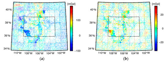
Figure 2.
(a) The original local gravity disturbance data; (b) the local gravity disturbance data after the GGM reduction and topographic reduction.
Parameterization area. To control edge effects, we refer to [9,28] to set the width between the parameterization area (the area covered by SRBFs) and the data area to . Thus, the parameterization area is bound by to and to .
Basis functions. In this study, the Shannon function is employed, with the Legendre coefficients defined as , ensuring that the signal is not smoothed within the corresponding spectral band. The maximum SH degree L of the basis functions is set to 2190, consistent with the SH degree of the local gravity disturbance data. The SRBFs are placed at the commonly used Reuter grid [20,29] points and the control parameter of the Reuter grid is set to 2190.
Model estimation. The functional model of the local gravity disturbance data can be represented as a linear Gauss–Markov model:
where denotes the vector of the local gravity disturbance dataset. and denote the design matrix and the NCM of the vector of the local gravity disturbance dataset, respectively. The vector consists of the model coefficient set , which is estimated using zero-order Tikhonov regularization [30]. Once the model coefficient set has been estimated, the single-scale model of the residual disturbing potential is given by Equation (A5). The residual height anomaly at any point within the target area can be computed based on the Bruns’ formula. To obtain the full signal of the height anomaly, it is necessary to restore the height anomaly signal from (1) the GOCO05s model complete to degree 280, (2) the XGM2016 model from degree 281 to 719, and (3) the dV_ELL_Earth2014 model from degree 720 to 2190.
3.3. Direct Approach
The experimental settings of the direct approach are the same as the classical RCR approach, except for the addition of a noisy satellite-only GGM dataset. Although the GOCO05s model complete to degree 280 is employed in the RCR procedure, the noisy GGM dataset consists of the SH coefficients of the GOCO05s model up to degree 230 and the corresponding NCMs. The purpose of this setup is to make the noisy GGM dataset used in the direct approach and the indirect approach consistent (see Section 3.4).
According to Equations (24) and (26), the functional model of the residual SH coefficients can be represented as a linear Gauss–Markov model:
where denotes the design matrix of the residual SH coefficients. Combining Equations (31) and (32) yields an overall linear Gauss–Markov model:
wherein
The model coefficients are still estimated using zero-order Tikhonov regularization.
3.4. Indirect Approach
The experimental settings of the indirect approach are inspired by [17,18]. The first step of the indirect approach is to estimate a single-scale model using the local gravity disturbance dataset and the classical RCR approach. The second step is to estimate a coarse-scale model using two datasets: one dataset consists of the height anomalies generated from the low-pass filtered GOCO05s model, and the other dataset consists of the height anomalies generated from the low-pass filtered single-scale model. The NCMs of the two datasets are both calculated according to the law of covariance propagation. It is worth noting that the generated GGM height anomalies do not contain any signal higher than degree 230. The reason is that the commission error of the GOCO05s model increases exponentially with the degree, and truncating the GOCO05s model at degree 230 is a compromise selection (see [7,18] for more details). Finally, the high-pass filtered single-scale model [18] is merged with the coarse-scale model to obtain an overall two-scale SRBF model. More details on the experimental settings of the indirect approach can be found in Appendix B.
4. Results and Discussion
4.1. Results
The height anomalies generated from the EIGEN-6C4 model up to degree 2190 are defined as truth values, with a resolution of distributed in the target area (between and and and ). We compare the quasi-geoid models calculated by different approaches with the truth values. Table 1 lists the statistics of the differences between the local quasi-geoid models and the truth values, while Figure 3 displays the spatial patterns of the differences. The numerical results show that the direct approach has superior performance. Compared to the classical RCR approach, the direct approach reduces the root-mean-square (RMS) error of the quasi-geoid model from 1.82 cm to 1.49 cm, which means that the model accuracy is improved by 18.1%. Figure 3a shows that in the northwest, northeast, and southeast of the target area, the quasi-geoid model calculated by the classical RCR approach exhibits large errors, which are caused by the sparse data distribution in these sub-areas (see Figure 1b). Instead, Figure 3b shows that the quasi-geoid model calculated by the direct approach effectively controls the prediction errors in the northwest and northeast of the target area and shows minor improvements in other areas as well, except for the southeast of the target area. The improvements of the direct approach on the local quasi-geoid model reflect the benefit of using satellite-only GGM as a noisy dataset.

Table 1.
Statistics of the differences between the quasi-geoid models and truth values (unit: cm).
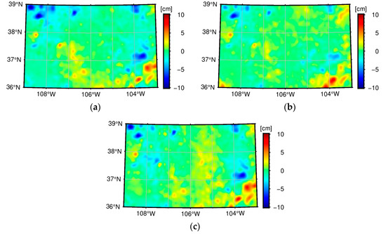
Figure 3.
Differences between the local quasi-geoid models and truth values. (a) Classical RCR approach; (b) direct approach; (c) indirect approach.
In terms of the RMS error of the quasi-geoid model, the indirect approach shows a slight improvement compared to the classical RCR approach (from 1.82 cm to 1.73 cm). Figure 3a,c show that in the northwest and northeast of the target area, the quasi-geoid model calculated by the indirect approach is slightly better than the quasi-geoid model calculated by the classical RCR approach. However, the situation is reversed in the central part of the target area. The indirect approach does not show the significant advantage of using satellite-only GGM as a noisy dataset. Figure 3b,c indicate that the quality of the quasi-geoid model calculated by the indirect approach is inferior to that calculated by the direct approach, especially in the central and eastern parts of the target area. In terms of the RMS error of the quasi-geoid model, the indirect approach is also inferior to the direct approach (1.73 cm vs. 1.49 cm).
4.2. Discussion
In Section 2, we demonstrated the theoretical equivalence of the direct approach and the indirect approach. However, in this study, the numerical results show that the direct approach outperforms the indirect approach. Slobbe et al. [18] attributed the poor performance of the indirect approach to the unreasonable relative weights between heterogeneous datasets. However, we tried different relative weights, but the results of the indirect approach were still not as good as the direct approach. The reason why the indirect approach does not perform as well as the direct approach may be related to the generation of the height anomaly dataset using satellite-only GGM. We generated very dense GGM height anomaly data and sufficiently expanded the parameterization area of the SRBFs, as shown in Appendix B. Nevertheless, the RMS of the differences between the height anomalies derived from the residual disturbing potential model estimated using the generated GGM height anomaly data and the control data is still greater than 0.3 cm. This may be related to the rough topography within the study area. Therefore, the generated height anomaly data are not an equivalent representation of the satellite-only GGM, which may lead to the loss of information from the satellite-only GGM. Instead, the direct approach directly uses the SH coefficients of the satellite-only GGM as a noisy dataset, effectively utilizing the information from the satellite-only GGM, which significantly improves the quality of the local quasi-geoid model.
5. Conclusions
In this study, we proposed an approach that directly uses the SH coefficients and the corresponding NCM of the satellite-only GGM as a noisy dataset and combines the GGM dataset and the local datasets to estimate the local quasi-geoid model. We have theoretically demonstrated the feasibility of the direct approach through mathematical deduction. Compared to the classical RCR approach, the direct approach achieves the optimal combination of local datasets with a noisy satellite-only GGM. We revisited the indirect approach and revealed the theoretical consistency between the direct approach and the indirect approach. However, compared to the indirect approach, the direct approach is more attractive due to its reliable results and low computational complexity. In the future, we will apply the direct approach to actual quasi-geoid modeling.
Author Contributions
Conceptualization, G.C.; methodology, G.C. and H.Y.; software, H.Y.; validation, H.Y.; formal analysis, H.Y. and G.C.; investigation, H.Y. and G.C.; resources, S.Z. and Y.Y.; data curation, H.Y. and Y.Y.; writing—original draft preparation, H.Y. and G.C.; writing—review and editing, H.Y. and G.C.; visualization, H.Y; supervision, G.C.; project administration, G.C. and S.Z.; funding acquisition, G.C., S.Z., and Y.Y. All authors have read and agreed to the published version of the manuscript.
Funding
This research was funded by the National Natural Science Foundation of China (Grant Nos. 42271460 and 42074001).
Data Availability Statement
The actual terrestrial gravity data and DEM of the study area are freely available at https://geodesy.noaa.gov/GEOID/research/co-cm-experiment/ (accessed on 22 January 2024).
Acknowledgments
The authors acknowledge the reviewers and editors for their comments, which helped us to greatly improve the manuscript significantly. The figures presented in this study were mainly generated using the Generic Mapping Tool [31].
Conflicts of Interest
The authors declare no conflicts of interest.
Appendix A. Two-Scale SRBF Model
The two-scale SRBF model has been described in detail in [7,18]. It is repeated here for the sake of completeness. After removing GGMs and topographic effects, the modeling object of the local gravity field is the residual disturbing potential. The residual disturbing potential can be represented by a two-scale SRBF model:
where and denote the number of SRBFs in the coarse-scale model and detailed-scale model, respectively. and denote the coefficient sets that need to be estimated. The basis functions and are given by
where is the maximum SH degree of the satellite-only GGM and . The filter coefficients are given by
where Equation (A4) is used as a low-pass filter, with parameters and determining the characteristics of the filter.
Given the particularity of the two-scale SRBF model, it is recommended to estimate the coefficient sets and in two steps to minimize signal leakage.
(1) Step 1: Based on the local gravity disturbance dataset, the detailed-scale model coefficient set is estimated using the classical RCR approach through the weighted least squares estimator. Furthermore, the coefficient set is also a coefficient set of the single-scale residual disturbing potential model estimated using the local gravity disturbance dataset, which is
The basis function in Equation (A5) is defined as
Note that the model coefficient set in Equation (A5) is identical to that in Equation (A1); however, the basis functions are different (cf. Equations (A3) and (A6)).
(2) Step 2: Calculate the weighted least squares estimation of the coarse-scale model coefficient set . The coarse-scale model is defined as
The model coefficient set is estimated based on two datasets: (1) the height anomaly dataset computed using the low-pass filtered satellite-only GGM; (2) the height anomaly dataset generated by the low-pass filtered single-scale model (cf. Equation (A5)). The low-pass filter coefficients are as shown in Equation (A4).
Appendix B. Experimental Settings of the Indirect Approach
Compared to the classical RCR approach and the direct approach, the computational procedure of the indirect approach is the most complex. We have configured the computation of the indirect approach following [17,18]. The first step of the indirect approach involves utilizing the local gravity disturbance dataset and employing the classic RCR approach to estimate the model coefficient set , which has already been completed. In the second step, the model coefficients set in (A7) will be estimated, and the computational details are as follows.
GGM height anomaly dat set. In the second step, it is necessary to redefine a data area and a parameterization area, both of which are specially customized for this step. The data area is bound by to and to , which is equivalent to extending the target area by . To compute the GGM height anomaly dataset, the filter coefficients from (A4) are first used to perform a low-pass filtering on the SH coefficients of the GOCO05s model. Here, the parameters and . Using SH synthesis, the filtered SH coefficients are used to calculate the height anomalies at the nodes within the data area. The NCM of the GGM height anomaly dataset is calculated from the NCM of the SH coefficients using the law of covariance propagation. The components of the GOCO05s model complete to degree 150 are removed from the height anomaly dataset, which is equivalent to using the GOCO05s model up to degree 150 as the reference GGM. The nodes of the height anomalies are located on the Reuter grid points on the Earth’s surface.
To reduce model errors (differences between the height anomalies derived from the SRBF model of the residual disturbing potential and control data), the control parameter of the Reuter grid and the extension of the parameterization area with respect to the data area need to be carefully defined. Klees et al. [17] showed that the model errors can be ignored when the control parameter of the Reuter grid is set to and the extension is . However, in this study, the terrain of the study area is extremely rugged, thus requiring a redefinition of these parameters through experiments. We placed the Shannon functions with a maximum SH degree of 230 on a Reuter grid with a control parameter of 230 and estimated residual disturbing potential models using the GGM height anomaly dataset generated at the nodes of a Reuter grid with different control parameters. To define the control data, we calculated a set of height anomaly data using the low-pass filtered GOCO05s model from degree 151 to 280 on an equal-angular grid of within the target area. We compared height anomalies derived from the residual disturbing potential models and the control data. Table A1 presents the statistics of model errors for different parameter settings. The numerical results indicate that the STD of the model errors is minimized when the extension of the parameterization area is and the control parameter of the Reuter grid is 690. At this time, the STD of the model errors is 0.33 cm, and the maximum absolute error of the model is comparable to the STDs of the GGM height anomaly data (1.4 cm to 1.5 cm). Figure A1 shows the spatial distribution of the model errors. It can be seen that there is a significant correlation between model errors and topography. The above findings indicate that it is difficult for the generated height anomaly dataset to preserve all the information of satellite-only GGM in mountainous areas with rough terrain. Therefore, the generated height anomaly dataset is not an equivalent representation of the satellite-only GGM. In statistical terms, the generated height anomaly dataset is not a sufficient statistic of the satellite-only GGM [32]. Based on the numerical results of the experiments, the parameterization area is bound by to and to , and the control parameter of the Reuter grid is set to 690.
Local height anomaly dataset. To compute the local height anomaly dataset, the filter coefficients from (A4) are first used to perform a low-pass filtering on the single-scale model shown in (A5). Here, the parameters and . Subsequently, the height anomalies are synthesized at the nodes within the data area, with the node positions being the same as those of the GGM height anomaly dataset. Due to the use of different reference GGMs in the first and second steps, we need to restore the low-pass filtered height anomaly signal of the GOCO05s model from degree 151 to 280. The NCM of the local height anomaly dataset is calculated from the NCM of the estimated model coefficient set using the law of covariance propagation.
Basis functions. In the second step, the Shannon function is still employed. The maximum SH degree of the basis functions is set to 230, consistent with the parameter . The SRBFs are still placed at the Reuter grid points and the control parameter of the Reuter grid is set to 230.
Model estimation. Due to the extreme ill-conditioning of the NCM of the GGM height anomaly dataset, the inversion-free weighted least-squares estimator [33] is introduced (see [18] for more details). Once the model coefficient sets and have been estimated, the two-scale SRBF model of the residual disturbing potential is given by (A1). The residual height anomaly at any point within the target area can be computed using the Bruns’ formula. To obtain the full signal of the height anomaly, it is necessary to restore the height anomaly signal from (1) the GOCO05s model up to degree 150, (2) the high-pass filtered GOCO05s model from degree 151 to 280, (3) the XGM2016 model from degree 281 to 719, and (4) the dV_ELL_Earth2014 model from degree 720 to 2190.
Table A1.
Statistics of model errors for different parameter settings. The control parameter of the Reuter grid is set to .
Table A1.
Statistics of model errors for different parameter settings. The control parameter of the Reuter grid is set to .
| Extension | SRBFs | Data Points | STD (cm) | Max (cm) | Min (cm) | Mean (cm) | |
|---|---|---|---|---|---|---|---|
| 1 | 92 | 92 | 1.09 | 4.20 | −3.73 | −0.15 | |
| 148 | 92 | 0.99 | 3.69 | −3.65 | −0.01 | ||
| 264 | 92 | 0.96 | 3.45 | −3.50 | 0.02 | ||
| 450 | 92 | 0.96 | 3.46 | −3.46 | −0.02 | ||
| 1.5 | 92 | 199 | 1.20 | 4.30 | −3.79 | 0.04 | |
| 148 | 199 | 0.38 | 1.49 | −2.28 | −0.05 | ||
| 264 | 199 | 0.37 | 1.42 | −2.11 | 0.04 | ||
| 450 | 199 | 0.38 | 1.51 | −2.05 | 0.05 | ||
| 2 | 92 | 364 | 1.53 | 5.66 | −5.51 | −0.03 | |
| 148 | 364 | 0.38 | 1.44 | −1.96 | −0.06 | ||
| 264 | 364 | 0.36 | 1.29 | −1.78 | −0.03 | ||
| 450 | 364 | 0.34 | 1.63 | −1.73 | 0.03 | ||
| 3 | 92 | 793 | 1.34 | 3.48 | −4.61 | −0.16 | |
| 148 | 793 | 0.37 | 1.53 | −2.11 | −0.02 | ||
| 264 | 793 | 0.34 | 1.53 | −1.84 | 0.03 | ||
| 5° | 450 | 793 | 0.33 | 1.41 | −1.68 | −0.01 |
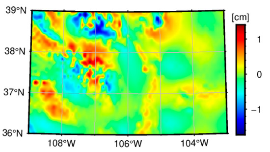
Figure A1.
Spatial distribution of the model errors.
References
- Ihde, J.; Sanchez, L.; Barzaghi, R.; Drewes, H.; Foerste, C.; Gruber, T.; Liebsch, G.; Marti, U.; Pail, R.; Sideris, M. Definition and Proposed Realization of the International Height Reference System (IHRS). Surv. Geophys. 2017, 38, 549–570. [Google Scholar] [CrossRef]
- Wang, Y.M.; Sanchez, L.; Agren, J.; Huang, J.L.; Forsberg, R.; Abd-Elmotaal, H.A.; Ahlgren, K.; Barzaghi, R.; Basic, T.; Carrion, D.; et al. Colorado geoid computation experiment: Overview and summary. J. Geod. 2021, 95, 127. [Google Scholar] [CrossRef]
- Farahani, H.H.; Ditmar, P.; Klees, R.; Liu, X.; Zhao, Q.; Guo, J. The static gravity field model DGM-1S from GRACE and GOCE data: Computation, validation and an analysis of GOCE mission’s added value. J. Geod. 2013, 87, 843–867. [Google Scholar] [CrossRef]
- Mayer-Gürr, T.; Pail, R.; Gruber, T.; Fecher, T.; Rexer, M.; Schuh, W.D.; Kusche, J.; Brockmann, J.M.; Rieser, D.; Zehentner, N.; et al. The combined satellite gravity field model GOCO05s. In Proceedings of the EGU General Assembly 2015, Vienna, Austria, 12–17 April 2015. [Google Scholar] [CrossRef]
- Kvas, A.; Brockmann, J.M.; Krauss, S.; Schubert, T.; Gruber, T.; Meyer, U.; Mayer-Gurr, T.; Schuh, W.D.; Jaggi, A.; Pail, R. GOCO06s-a satellite-only global gravity field model. Earth Syst. Sci. Data 2021, 13, 99–118. [Google Scholar] [CrossRef]
- Forsberg, R.; Tscherning, C.C. The use of height data in gravity field approximation by collocation. J. Geophys. Res. Solid Earth 1981, 86, 7843–7854. [Google Scholar] [CrossRef]
- Klees, R.; Slobbe, D.C.; Farahani, H.H. A methodology for least-squares local quasi-geoid modelling using a noisy satellite-only gravity field model. J. Geod. 2018, 92, 431–442. [Google Scholar] [CrossRef]
- Lin, M.; Denker, H.; Muller, J. A comparison of fixed- and free-positioned point mass methods for regional gravity field modeling. J. Geodyn. 2019, 125, 32–47. [Google Scholar] [CrossRef]
- Liu, Q.; Schmidt, M.; Sanchez, L.; Willberg, M. Regional gravity field refinement for (quasi-) geoid determination based on spherical radial basis functions in Colorado. J. Geod. 2020, 94, 99. [Google Scholar] [CrossRef]
- Li, X.P. Using radial basis functions in airborne gravimetry for local geoid improvement. J. Geod. 2018, 92, 471–485. [Google Scholar] [CrossRef]
- Denker, H. Regional Gravity Field Modeling: Theory and Practical Results. In Sciences of Geodesy—II: Innovations and Future Developments; Xu, G., Ed.; Springer: Berlin/Heidelberg, Germany, 2013; pp. 185–291. [Google Scholar] [CrossRef]
- Jiang, T.; Wang, Y.M. On the spectral combination of satellite gravity model, terrestrial and airborne gravity data for local gravimetric geoid computation. J. Geod. 2016, 90, 1405–1418. [Google Scholar] [CrossRef]
- Jiang, T.; Dang, Y.; Zhang, C. Gravimetric geoid modeling from the combination of satellite gravity model, terrestrial and airborne gravity data: A case study in the mountainous area, Colorado. Earth Planets Space 2020, 72, 189. [Google Scholar] [CrossRef]
- Willberg, M.; Zingerle, P.; Pail, R. Residual least-squares collocation: Use of covariance matrices from high-resolution global geopotential models. J. Geod. 2019, 93, 1739–1757. [Google Scholar] [CrossRef]
- Willberg, M.; Zingerle, P.; Pail, R. Integration of airborne gravimetry data filtering into residual least-squares collocation: Example from the 1 cm geoid experiment. J. Geod. 2020, 94, 75. [Google Scholar] [CrossRef]
- Lieb, V.; Schmidt, M.; Dettmering, D.; Boerger, K. Combination of various observation techniques for regional modeling of the gravity field. J. Geophys. Res. Solid Earth 2016, 121, 3825–3845. [Google Scholar] [CrossRef]
- Klees, R.; Slobbe, D.C.; Farahani, H.H. How to deal with the high condition number of the noise covariance matrix of gravity field functionals synthesised from a satellite-only global gravity field model? J. Geod. 2019, 93, 29–44. [Google Scholar] [CrossRef]
- Slobbe, C.; Klees, R.; Farahani, H.H.; Huisman, L.; Alberts, B.; Voet, P.; De Doncker, F. The Impact of Noise in a GRACE/GOCE Global Gravity Model on a Local Quasi-Geoid. J. Geophys. Res. Solid Earth 2019, 124, 3219–3237. [Google Scholar] [CrossRef]
- Schmidt, M.; Fengler, M.; Mayer-Gurr, T.; Eicker, A.; Kusche, J.; Sanchez, L.; Han, S.C. Regional gravity modeling in terms of spherical base functions. J. Geod. 2007, 81, 17–38. [Google Scholar] [CrossRef]
- Eicker, A. Gravity Field Refinement by Radial Basis Functions from In-Situ Satellite Data. Ph.D. Thesis, Bonn University, Bonn, Germany, 2008. [Google Scholar]
- Heiskanen, W.A.; Moritz, H. Physical Geodesy; W.H. Freeman and Company: San Francisco, CA, USA, 1967. [Google Scholar]
- Bucha, B.; Janak, J.; Papco, J.; Bezdek, A. High-resolution regional gravity field modelling in a mountainous area from terrestrial gravity data. Geophys. J. Int. 2016, 207, 949–966. [Google Scholar] [CrossRef]
- Wittwer, T. Regional Gravity Field Modelling with Radial Basis Functions. Ph.D. Thesis, Delft University of Technology, Delft, The Nederland, 2009. [Google Scholar]
- Förste, C.; Bruinsma, S.L.; Abrikosov, O.; Lemoine, J.M.; Marty, J.C.; Flechtner, F.; Balmino, G.; Barthelmes, F.; Biancale, R. EIGEN-6C4 the Latest Combined Global Gravity Field Model Including GOCE Data up to Degree and Order 2190 of GFZ Potsdam and GRGS Toulouse. GFZ Data Services, 2014. [Google Scholar] [CrossRef]
- Pail, R.; Fecher, T.; Barnes, D.; Factor, J.F.; Holmes, S.A.; Gruber, T.; Zingerle, P. Short note: The experimental geopotential model XGM2016. J. Geod. 2018, 92, 443–451. [Google Scholar] [CrossRef]
- Yu, H.P.; Chang, G.B.; Zhang, S.B.; Zhu, Y.H.; Yu, Y.J. Application of Sparse Regularization in Spherical Radial Basis Functions-Based Regional Geoid Modeling in Colorado. Remote Sens. 2023, 15, 4870. [Google Scholar] [CrossRef]
- Rexer, M.; Hirt, C.; Claessens, S.; Tenzer, R. Layer-Based Modelling of the Earth’s Gravitational Potential up to 10-km Scale in Spherical Harmonics in Spherical and Ellipsoidal Approximation. Surv. Geophys. 2016, 37, 1035–1074. [Google Scholar] [CrossRef]
- Ma, Z.; Yang, M.; Liu, J. Regional Gravity Field Modeling Using Band-Limited SRBFs: A Case Study in Colorado. Remote Sens. 2023, 15, 4515. [Google Scholar] [CrossRef]
- Reuter, R. Über Integralformeln der Einheitssphäre und Harmonische Splinefunktionen. Ph.D. Thesis, RWTH Aachen University, Aachen, Germany, 1982. [Google Scholar]
- Tikhonov, A.N. Solution of incorrectly formulated problems and the regularization method. Sov. Math. Dokl. 1963, 4, 1035–1038. [Google Scholar]
- Wessel, P.; Luis, J.F.; Uieda, L.; Scharroo, R.; Wobbe, F.; Smith, W.H.F.; Tian, D. The Generic Mapping Tools Version 6. Geochem. Geophy. Geosy. 2019, 20, 5556–5564. [Google Scholar] [CrossRef]
- Kay, S.M. Fundamentals of Statistical Signal Processing, Volume I: Estimation Theory; Pearson Education: New York, NY, USA, 2013. [Google Scholar]
- Grafarend, E.W.; Schaffrin, B. Ausgleichungsrechnung in Linearen Modellen; BI-Wissenschaftsverlag: Mannheim, Germany, 1993. [Google Scholar]
Disclaimer/Publisher’s Note: The statements, opinions and data contained in all publications are solely those of the individual author(s) and contributor(s) and not of MDPI and/or the editor(s). MDPI and/or the editor(s) disclaim responsibility for any injury to people or property resulting from any ideas, methods, instructions or products referred to in the content. |
© 2024 by the authors. Licensee MDPI, Basel, Switzerland. This article is an open access article distributed under the terms and conditions of the Creative Commons Attribution (CC BY) license (https://creativecommons.org/licenses/by/4.0/).