
Trend Classification of InSAR Displacement Time Series Using SAE–CNN


Abstract
:
1. Introduction
2. Materials and Methods
2.1. Predefined Types of Displacement Time Series
- Stable: This trend represents areas where no significant deformation is observed. This class contains non-moving targets (green points in Figure 2).
- Linear: This class contains points with deformation that constantly increase or decrease over time. These points have a constant velocity in the time series (yellow points in Figure 2).
- Accelerating: The accelerating class shows continuous movements and can be characterized by an increasing deformation rate in the time series (red trend in Figure 2). The deformation time series can be approximated by two linear sub-periods with different rates or a second-order polynomial.
- Decelerating: The decelerating displacement class is also nonlinear, with a decreasing deformation rate over time. The final deformation rate can be reduced to zero, that is, stable.
- Phase unwrapping error (PUE): This trend includes TS affected by abnormal deformation jumps caused by PUE in InSAR processing (black points in Figure 2). The PUE value, a multiple of half the wavelength, approximately 28.3 mm in Sentinel-1 SAR images, may change with the noise. TSs affected by vertical jumps greater than 15 mm are classified as PUE [23].
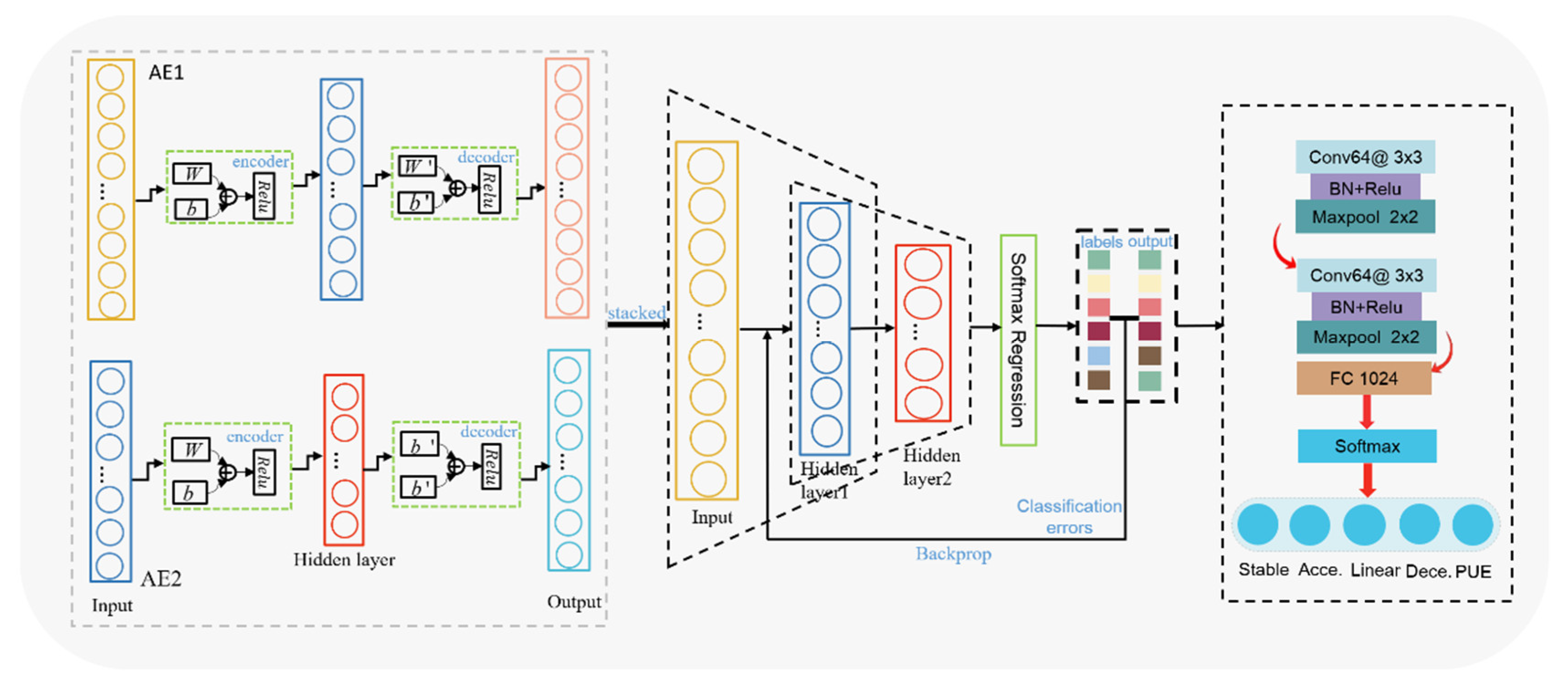
2.2. The Classification Network That Combines the Optimal SAE and CNN
2.3. Accuracy Assessments
3. Study Area and Datasets
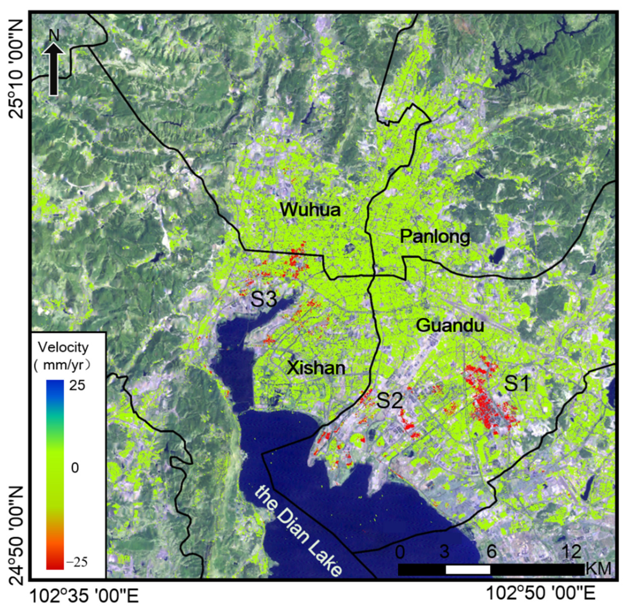
3.1. Study Area
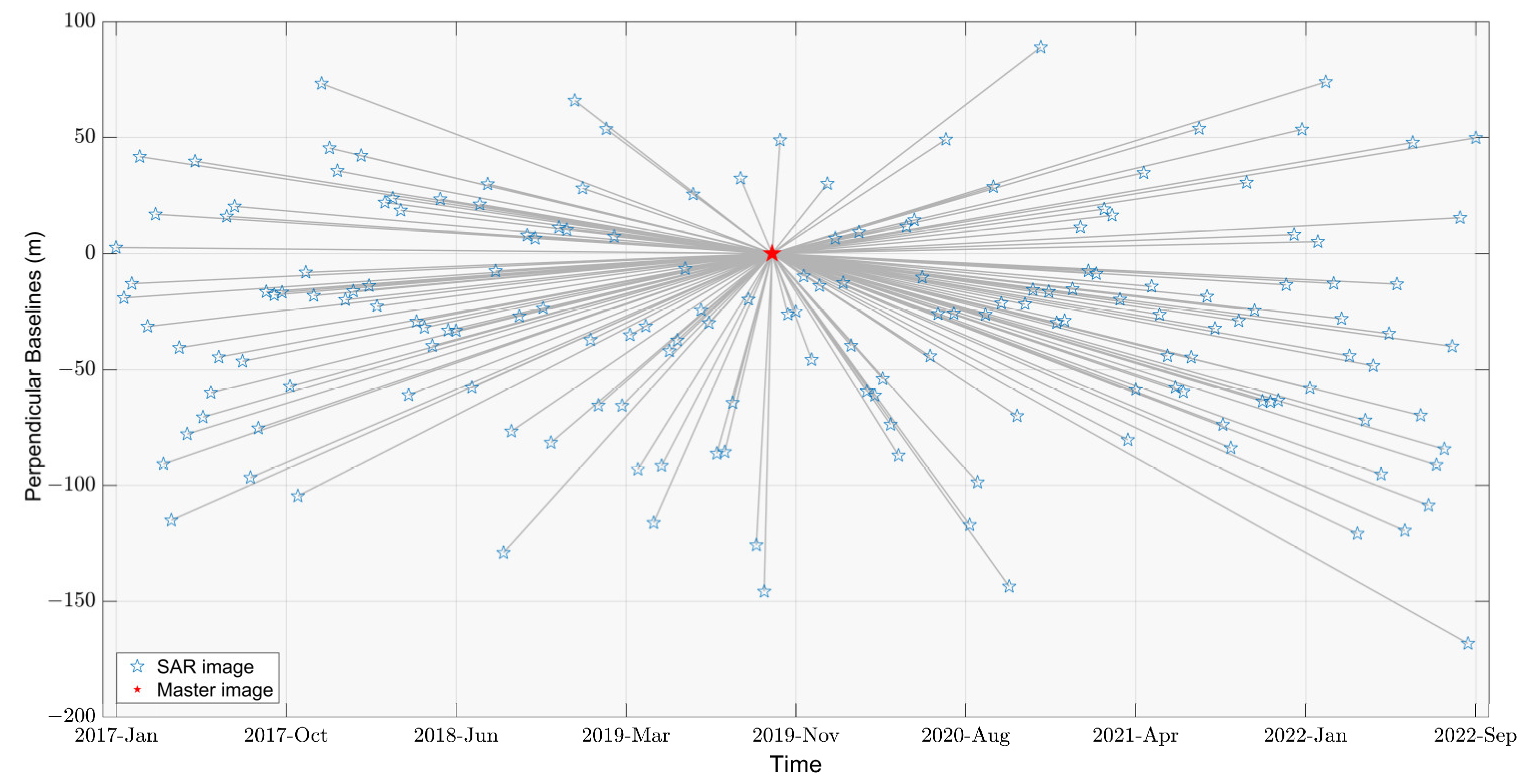
3.2. Datasets
4. Results and Analysis
4.1. Validation of the Proposed Classifier
4.2. SAE Model Analysis
4.3. Classification of the InSAR TS in Kunming
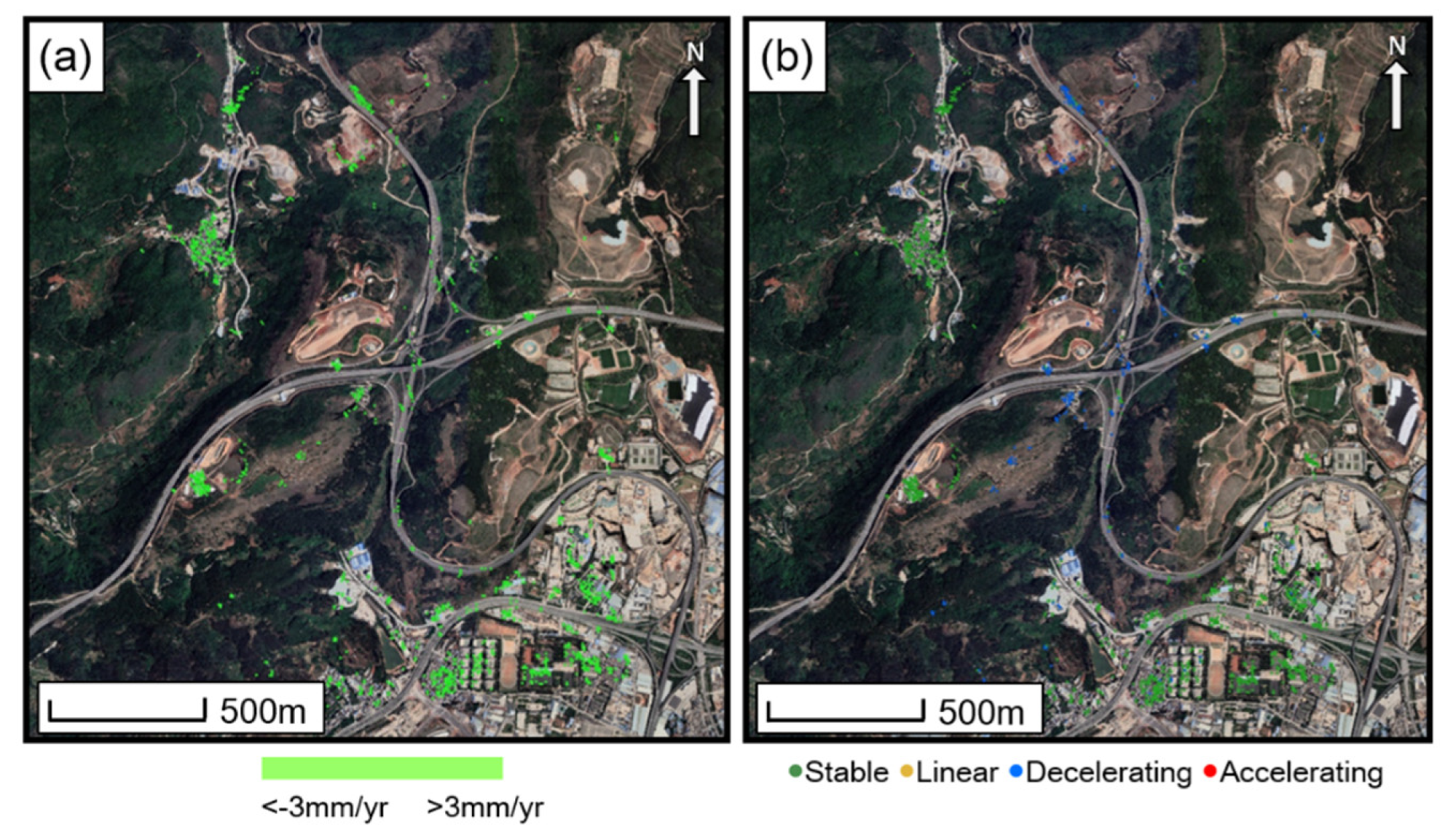
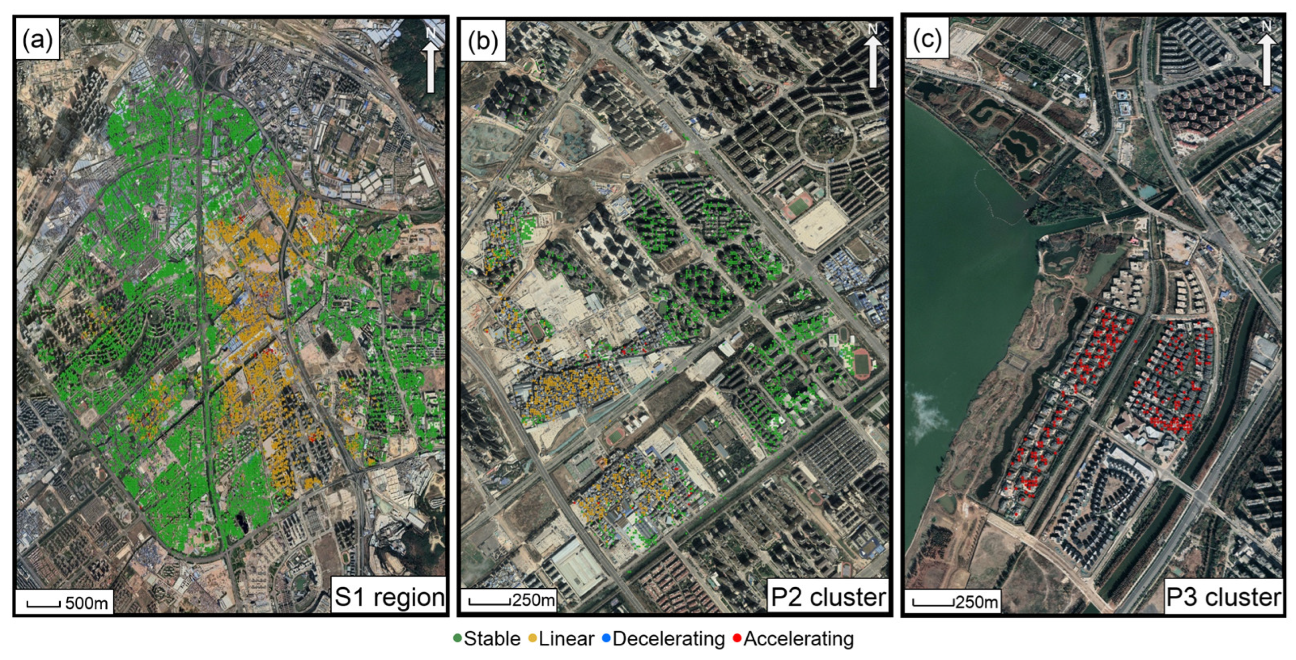
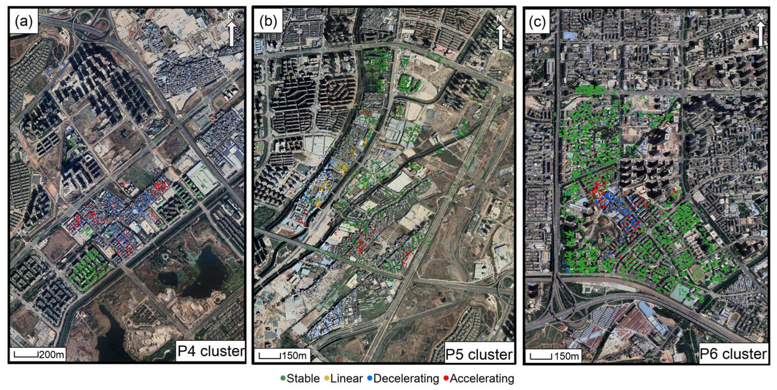
4.4. Analysis of the InSAR Classification Map
5. Discussion
6. Conclusions
Author Contributions
Funding
Data Availability Statement
Conflicts of Interest
References
- Crosetto, M.; Monserrat, O.; Cuevas-González, M.; Devanthéry, N.; Crippa, B. Persistent Scatterer Interferometry: A review. ISPRS J. Photogramm. Remote Sens. 2016, 115, 78–89. [Google Scholar] [CrossRef]
- Li, S.; Xu, W.; Li, Z. Review of the SBAS InSAR Time-series algorithms, applications, and challenges. Geod. Geodyn. 2022, 13, 114–126. [Google Scholar] [CrossRef]
- Li, M.; Zhang, L.; Yang, M.; Liao, M. Complex surface displacements of the Nanyu landslide in Zhouqu, China revealed by multi-platform InSAR observations. Eng. Geol. 2023, 317, 107069. [Google Scholar] [CrossRef]
- Yang, M.; Wang, R.; Li, M.; Liao, M. A PSI targets characterization approach to interpreting surface displacement signals: A case study of the Shanghai metro tunnels. Remote Sens. Environ. 2022, 280, 113150. [Google Scholar] [CrossRef]
- Cigna, F.; Tapete, D.; Casagli, N. Semi-automated extraction of Deviation Indexes (DI) from satellite Persistent Scatterers time series: Tests on sedimentary volcanism and tectonically-induced motions. Nonlinear Process Geophys. 2012, 19, 643–655. [Google Scholar] [CrossRef]
- Berti, M.; Corsini, A.; Franceschini, S.; Iannacone, J.P. Automated classification of Persistent Scatterers Interferometry time series. Nat. Hazards Earth Syst. Sci. 2013, 13, 1945–1958. [Google Scholar] [CrossRef]
- Tomás, R.; Li, Z.; Lopez-Sanchez, J.M.; Liu, P.; Singleton, A. Using wavelet tools to analyse seasonal variations from InSAR time-series data: A case study of the Huangtupo landslide. Landslides 2016, 13, 437–450. [Google Scholar] [CrossRef]
- Chang, L.; Hanssen, R.F. A Probabilistic Approach for InSAR Time-Series Postprocessing. IEEE Trans. Geosci. Remote Sens. 2016, 54, 421–430. [Google Scholar] [CrossRef]
- Bovenga, F.; Pasquariello, G.; Refice, A. Statistically-Based Trend Analysis of MTInSAR Displacement Time Series. Remote Sens. 2021, 13, 2302. [Google Scholar] [CrossRef]
- Refice, A.; Pasquariello, G.; Bovenga, F. Model-Free Characterization of SAR MTI Time Series. IEEE Geosci. Remote Sens. Lett. 2022, 19, 1–5. [Google Scholar] [CrossRef]
- Brengman, C.M.J.; Barnhart, W.D. Identification of Surface Deformation in InSAR Using Machine Learning. Geochem. Geophys. Geosystems 2021, 22, e2020GC009204. [Google Scholar] [CrossRef]
- Rouet-Leduc, B.; Jolivet, R.; Dalaison, M.; Johnson, P.A.; Hulbert, C. Autonomous extraction of millimeter-scale deformation in InSAR time series using deep learning. Nat. Commun. 2021, 12, 6480. [Google Scholar] [CrossRef] [PubMed]
- Novellino, A.; Cesarano, M.; Cappelletti, P.; Di Martire, D.; Di Napoli, M.; Ramondini, M.; Sowter, A.; Calcaterra, D. Slow-moving landslide risk assessment combining Machine Learning and InSAR techniques. Catena 2021, 203, 105317. [Google Scholar] [CrossRef]
- Zhou, H.; Dai, K.; Pirasteh, S.; Li, R.; Xiang, J.; Li, Z. InSAR Spatial-Heterogeneity Tropospheric Delay Correction in Steep Mountainous Areas Based on Deep Learning for Landslides Monitoring. IEEE Trans. Geosci. Remote Sens. 2023, 61, 1–14. [Google Scholar] [CrossRef]
- Shakeel, A.; Walters, R.J.; Ebmeier, S.K.; Moubayed, N.A. ALADDIn: Autoencoder-LSTM-Based Anomaly Detector of Deformation in InSAR. IEEE Trans. Geosci. Remote Sens. 2022, 60, 4706512. [Google Scholar] [CrossRef]
- Ansari, H.; Rubwurm, M.; Ali, M.; Montazeri, S.; Parizzi, A.; Zhu, X.X. InSAR Displacement Time Series Mining: A Machine Learning Approach. In Proceedings of the 2021 IEEE International Geoscience and Remote Sensing Symposium IGARSS, Brussels, Belgium, 11–16 July 2021; pp. 3301–3304. [Google Scholar]
- Martin, G.; Selvakumaran, S.; Marinoni, A.; Sadeghi, Z.; Middleton, C. Structural Health Monitoring on Urban Areas by Using Multi Temporal Insar and Deep Learning. In Proceedings of the 2021 IEEE International Geoscience and Remote Sensing Symposium IGARSS, Brussels, Belgium, 11–16 July 2021; pp. 176–179. [Google Scholar]
- van de Kerkhof, B.; Pankratius, V.; Chang, L.; van Swol, R.; Hanssen, R.F. Individual Scatterer Model Learning for Satellite Interferometry. IEEE Trans. Geosci. Remote Sens. 2020, 58, 1273–1280. [Google Scholar] [CrossRef]
- Festa, D.; Novellino, A.; Hussain, E.; Bateson, L.; Casagli, N.; Confuorto, P.; Del Soldato, M.; Raspini, F. Unsupervised detection of InSAR time series patterns based on PCA and K-means clustering. Int. J. Appl. Earth Obs. Geoinf. 2023, 118, 103276. [Google Scholar] [CrossRef]
- Rygus, M.; Novellino, A.; Hussain, E.; Syafiudin, F.; Andreas, H.; Meisina, C. A clustering approach for the analysis of InSAR Time Series: Application to the Bandung Basin (Indonesia). Remote Sens. 2023, 15, 3776. [Google Scholar] [CrossRef]
- Kulshrestha, A.; Chang, L.; Stein, A. Use of LSTM for sinkhole-related anomaly detection and classification of InSAR deformation time series. IEEE J. Sel. Top. Appl. Earth Obs. Remote Sens. 2022, 15, 4559–4570. [Google Scholar] [CrossRef]
- Mirmazloumi, S.M.; Gambin, A.F.; Palamà, R.; Crosetto, M.; Wassie, Y.; Navarro, J.A.; Barra, A.; Monserrat, O. Supervised Machine Learning Algorithms for Ground Motion Time Series Classification from InSAR Data. Remote Sens. 2022, 14, 3821. [Google Scholar] [CrossRef]
- Mirmazloumi, S.M.; Wassie, Y.; Navarro, J.A.; Palamà, R.; Krishnakumar, V.; Barra, A.; Cuevas-González, M.; Crosetto, M.; Monserrat, O. Classification of ground deformation using sentinel-1 persistent scatterer interferometry time series. GIScience Remote Sens. 2022, 59, 374–392. [Google Scholar] [CrossRef]
- Wang, C.; Han, F.; Zhang, Y.; Lu, J. An SAE-based resampling SVM ensemble learning paradigm for pipeline leakage detection. Neurocomputing 2020, 403, 237–246. [Google Scholar] [CrossRef]
- Kingma, D.P.; Ba, J. Adam: A Method for Stochastic Optimization. arXiv 2014, arXiv:1412.6980. [Google Scholar]
- Yang, B.; Liu, H. Automatic identification of insomnia based on single-channel EEG labelled with sleep stage annotations. IEEE Access 2020, 8, 104281–104291. [Google Scholar] [CrossRef]
- Jung, W.; Jung, D.; Kim, B.; Lee, S.; Rhee, W.; Ahn, J.H. Restructuring batch normalization to accelerate CNN training. Proc. Mach. Learn. Syst. 2019, 1, 14–26. [Google Scholar]
- Novaković, J.D.; Veljović, A.; Ilić, S.S.; Papić, Ž.; Tomović, M. Evaluation of classification models in machine learning. Theory Appl. Math. Comput. Sci. 2017, 7, 39. [Google Scholar]
- Li, Y.; Yang, X.; Wu, B.; Zhao, J.; Jiang, W.; Feng, X.; Li, Y. Spatio-temporal evolution and prediction of carbon storage in Kunming based on PLUS and InVEST models. PeerJ 2023, 11, e15285. [Google Scholar] [CrossRef]
- Zhu, W.; Li, W.L.; Zhang, Q.; Yang, Y.; Zhang, Y.; Qu, W.; Wang, C.S. A Decade of Ground Deformation in Kunming (China) Revealed by Multi-Temporal Synthetic Aperture Radar Interferometry (InSAR) Technique. Sensors 2019, 19, 4425. [Google Scholar] [CrossRef]
- Li, M.; Yin, X.; Tang, B.-H.; Yang, M. Accuracy Assessment of High-Resolution Globally Available Open-Source DEMs Using ICESat/GLAS over Mountainous Areas, A Case Study in Yunnan Province, China. Remote Sens. 2023, 15, 1952. [Google Scholar] [CrossRef]
- Hooper, A.; Zebker, H.; Segall, P.; Kampes, B. A new method for measuring deformation on volcanoes and other natural terrains using InSAR persistent scatterers. Geophys. Res. Lett. 2004, 31, 1–5. [Google Scholar] [CrossRef]
- Hooper, A.; Segall, P.; Zebker, H. Persistent scatterer interferometric synthetic aperture radar for crustal deformation analysis, with application to Volcán Alcedo, Galápagos. J. Geophys. Res. 2007, 2156–2202, 2156–2202. [Google Scholar] [CrossRef]
- Li, S.; Wang, Z.; Yuan, L.; Li, X.; Huang, Y.; Guo, R. Mechanism of Land Subsidence of Plateau Lakeside Kunming City Cluster (China) by MT-InSAR and Leveling Survey. J. Coast. Res. 2020, 115, 666–675. [Google Scholar] [CrossRef]
- Wang, J.; Li, M.; Yang, M.; Tang, B.-H. Deformation Detection and Attribution Analysis of Urban Areas near Dianchi Lake in Kunming Using the Time-Series InSAR Technique. Appl. Sci. 2022, 12, 10004. [Google Scholar] [CrossRef]
- Shao, J.; Li, J.; Yang, K. Time-Series Analysis of Land Subsidence in Kunming. In Proceedings of the 2018 Eighth International Conference on Instrumentation & Measurement, Computer, Communication and Control (IMCCC), Harbin, China, 19–21 July 2018; pp. 295–298. [Google Scholar] [CrossRef]
- Belkina, A.C.; Ciccolella, C.O.; Anno, R.; Halpert, R.; Spidlen, J.; Snyder-Cappione, J.E. Automated optimized parameters for T-distributed stochastic neighbor embedding improve visualization and analysis of large datasets. Nat. Commun. 2019, 10, 5415. [Google Scholar] [CrossRef]
- Guo, S.; Kang, W.; Zhang, T.; Li, Y. The Study on Land Subsidence in Kunming by Integrating PS, SBAS and DS InSAR. Remote Sens.Technol. Appl. 2022, 37, 460–473. [Google Scholar] [CrossRef]


| Description | Value |
|---|---|
| Number of hidden layers | 3 |
| Number of neurons in each hidden layer | 256/128/64 |
| Activation function | Relu |
| Learning rate | 1e−4 |
| Batch size | 128 |
| Layer Type | Filter_Num | Kernel Size | Region Size | Output Size | |
|---|---|---|---|---|---|
| Part1 | 1D-CNN | 64 | 3 × 3 | - | (64, 64) |
| BatchNorm | 64 | - | - | (64, 64) | |
| MaxPool | - | - | 2 × 2 | (32, 64) | |
| Part2 | 1D-CNN | 64 | 3 × 3 | - | (32, 64) |
| BatchNorm | 64 | - | - | (32, 64) | |
| MaxPool | - | - | 2 × 2 | (16, 64) | |
| FC | Flatten | - | - | 1024 | 1024 |
| Softmax | - | - | 5 | 5 |
| Model | Accuracy | Precision | Recall | F1-Score | |
|---|---|---|---|---|---|
| 1 | the proposed | 0.951 | 0.953 | 0.952 | 0.952 |
| 2 | CNN | 0.887 | 0.897 | 0.887 | 0.891 |
| 3 | RF | 0.878 | 0.889 | 0.879 | 0.883 |
| 4 | SVC | 0.832 | 0.858 | 0.836 | 0.846 |
| Model | Time (s) |
|---|---|
| the Proposed | 32.18 |
| CNN | 3.36 |
| RF | 1.69 |
| SVC | 413.46 |
Disclaimer/Publisher’s Note: The statements, opinions and data contained in all publications are solely those of the individual author(s) and contributor(s) and not of MDPI and/or the editor(s). MDPI and/or the editor(s) disclaim responsibility for any injury to people or property resulting from any ideas, methods, instructions or products referred to in the content. |
© 2023 by the authors. Licensee MDPI, Basel, Switzerland. This article is an open access article distributed under the terms and conditions of the Creative Commons Attribution (CC BY) license (https://creativecommons.org/licenses/by/4.0/).
Share and Cite
Li, M.; Wu, H.; Yang, M.; Huang, C.; Tang, B.-H. Trend Classification of InSAR Displacement Time Series Using SAE–CNN. Remote Sens. 2024, 16, 54. https://doi.org/10.3390/rs16010054
Li M, Wu H, Yang M, Huang C, Tang B-H. Trend Classification of InSAR Displacement Time Series Using SAE–CNN. Remote Sensing. 2024; 16(1):54. https://doi.org/10.3390/rs16010054
Chicago/Turabian StyleLi, Menghua, Hanfei Wu, Mengshi Yang, Cheng Huang, and Bo-Hui Tang. 2024. "Trend Classification of InSAR Displacement Time Series Using SAE–CNN" Remote Sensing 16, no. 1: 54. https://doi.org/10.3390/rs16010054
APA StyleLi, M., Wu, H., Yang, M., Huang, C., & Tang, B.-H. (2024). Trend Classification of InSAR Displacement Time Series Using SAE–CNN. Remote Sensing, 16(1), 54. https://doi.org/10.3390/rs16010054