
Characterizing the Water Storage Variation of Kusai Lake by Constructing Time Series from Multisource Remote Sensing Data

 ,
,  and
and
Abstract
:
1. Introduction
2. Materials
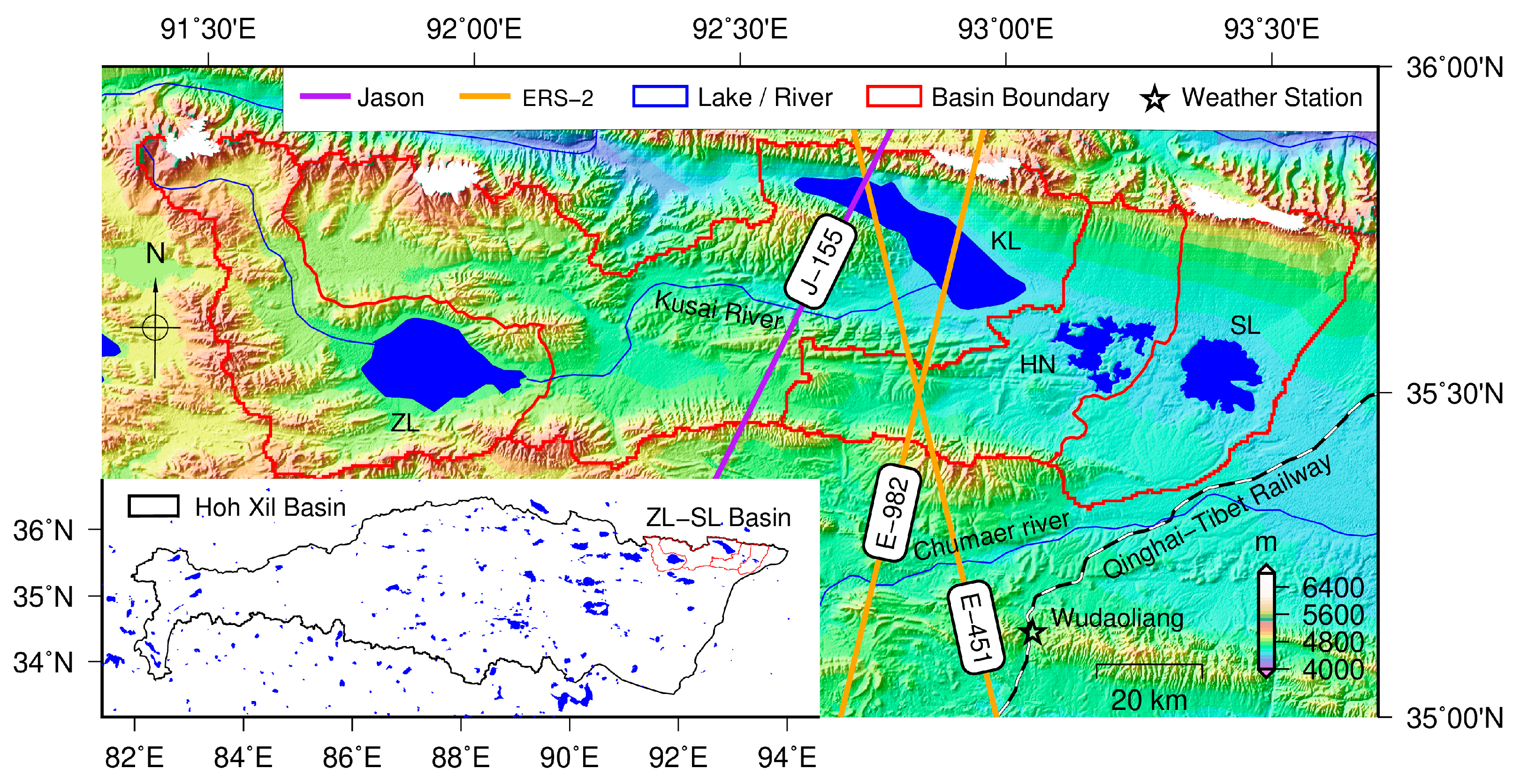
2.1. Study Area
2.2. Data
2.2.1. Satellite Altimeter Data
2.2.2. Remote Sensing Images
2.2.3. Topographic Data
2.2.4. Ancillary Data
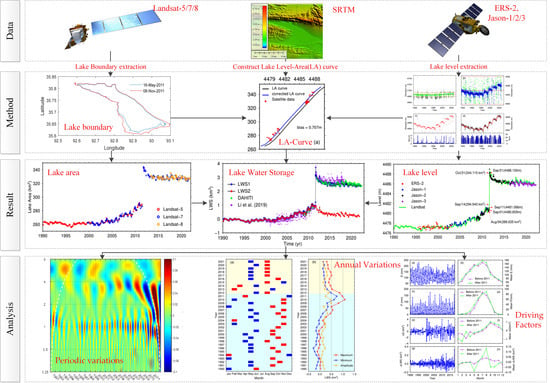
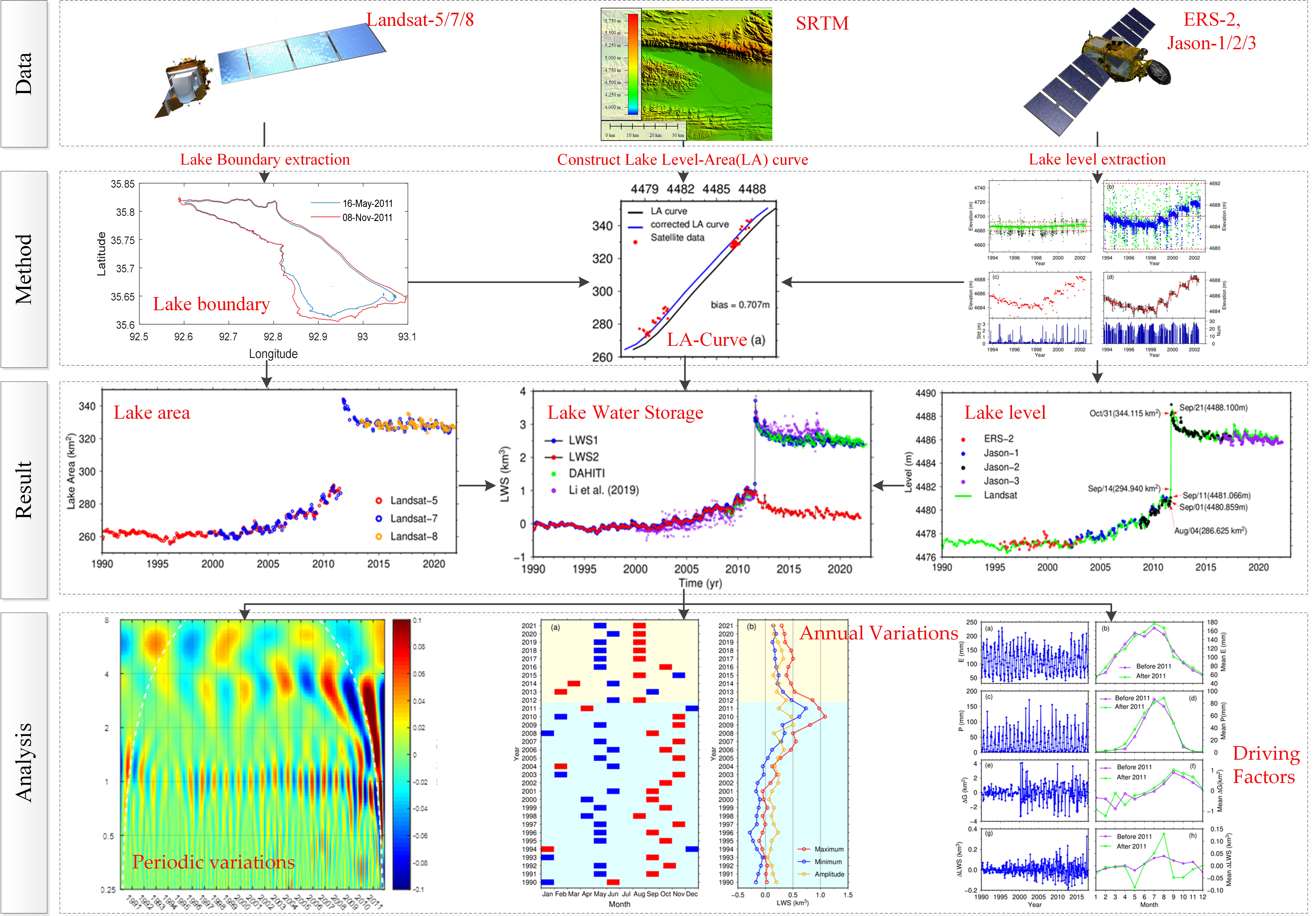
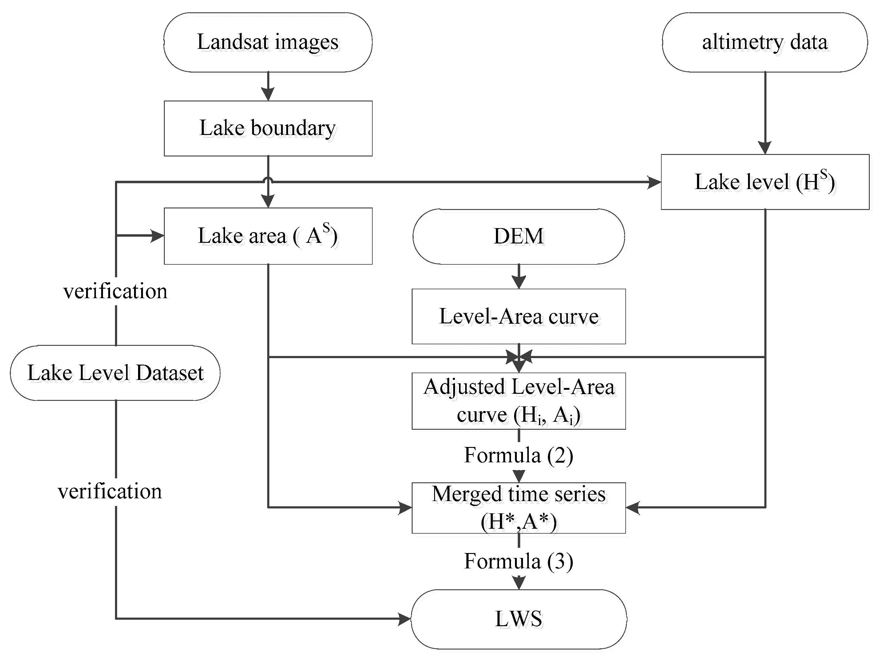
3. Methods
3.1. Monitoring Lake Changes Based on Satellite Technology
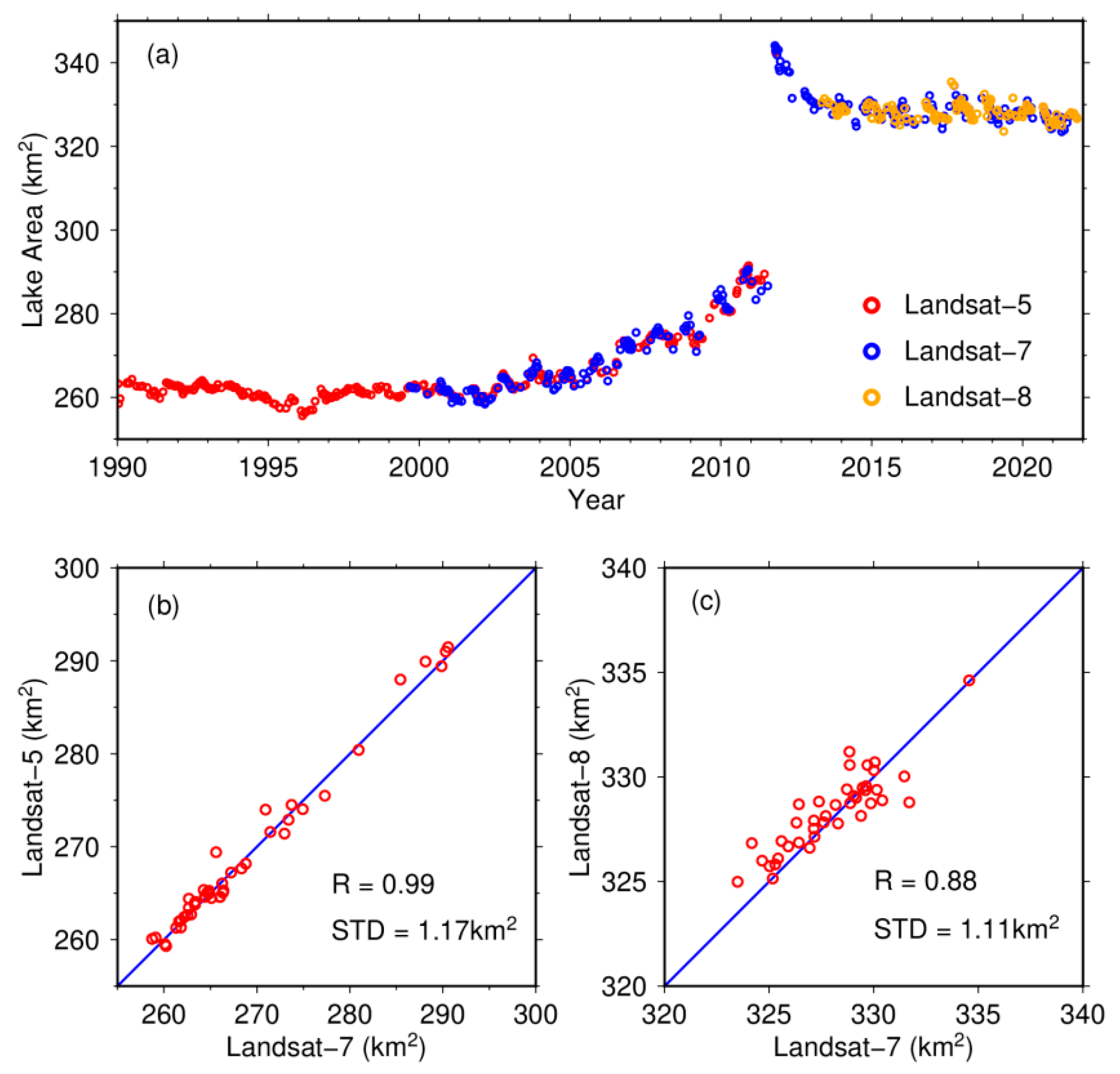
3.1.1. Estimation of Lake Areas from Landsat Images
3.1.2. Extraction of Lake Levels from Altimeter Data
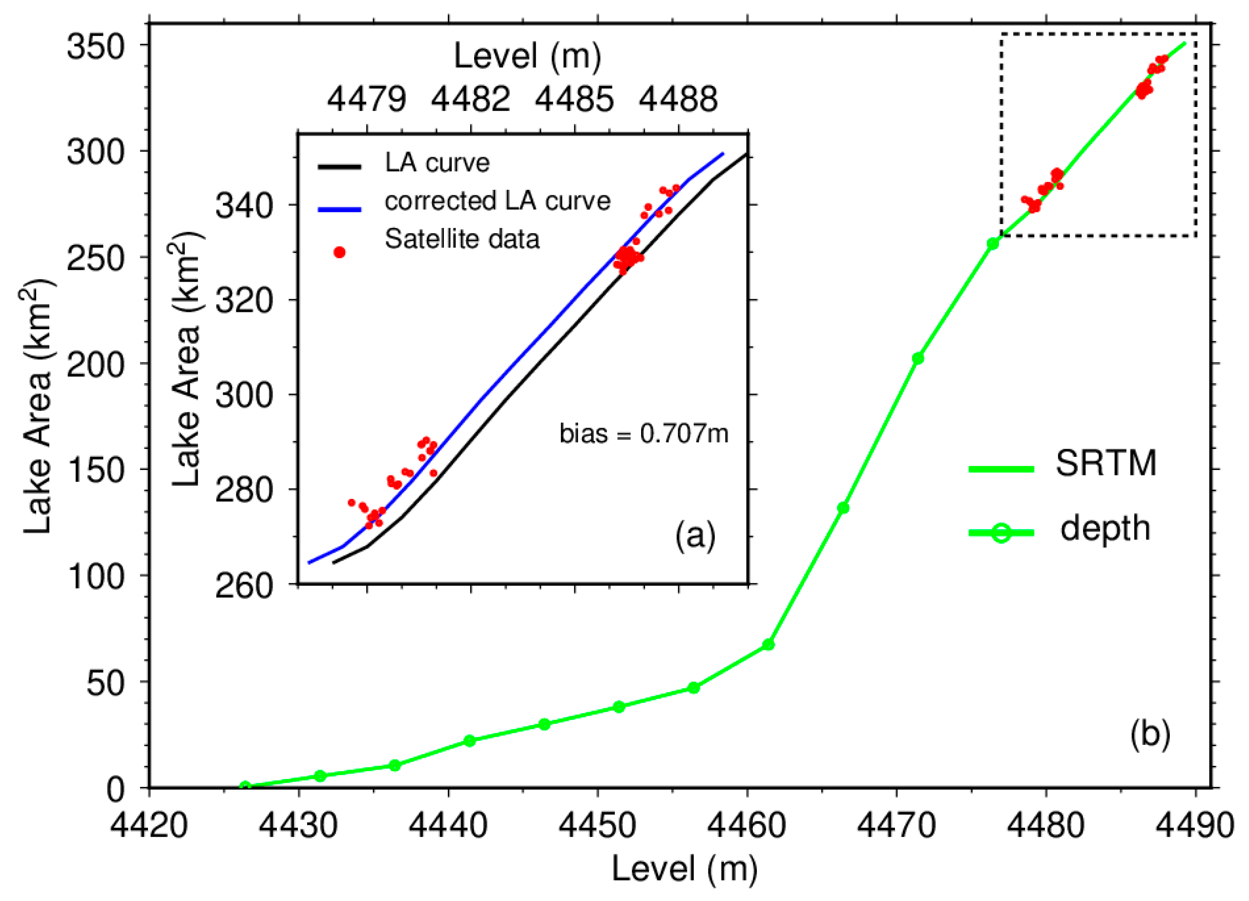
3.2. Construction of Lake Water Level-Area (LA) Curve
3.3. Interpolation between Lake Level and Area
3.4. Computation of Lake Water Storage (LWS)
4. Results and Validations
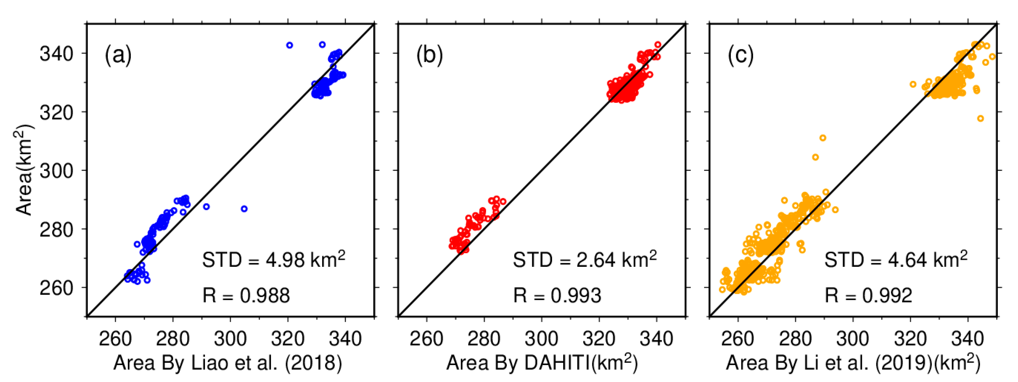
4.1. Lake Area
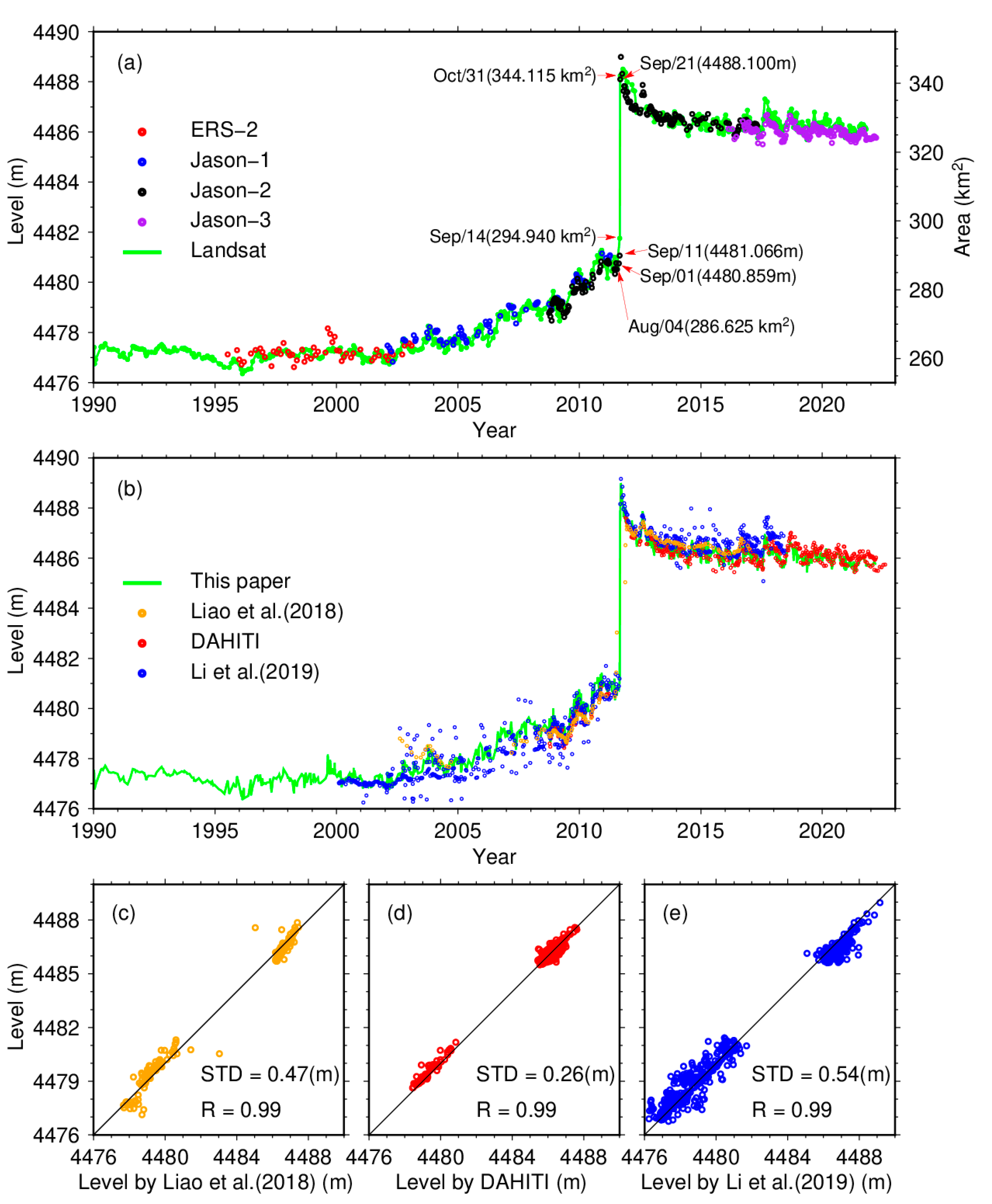
4.2. Lake Level
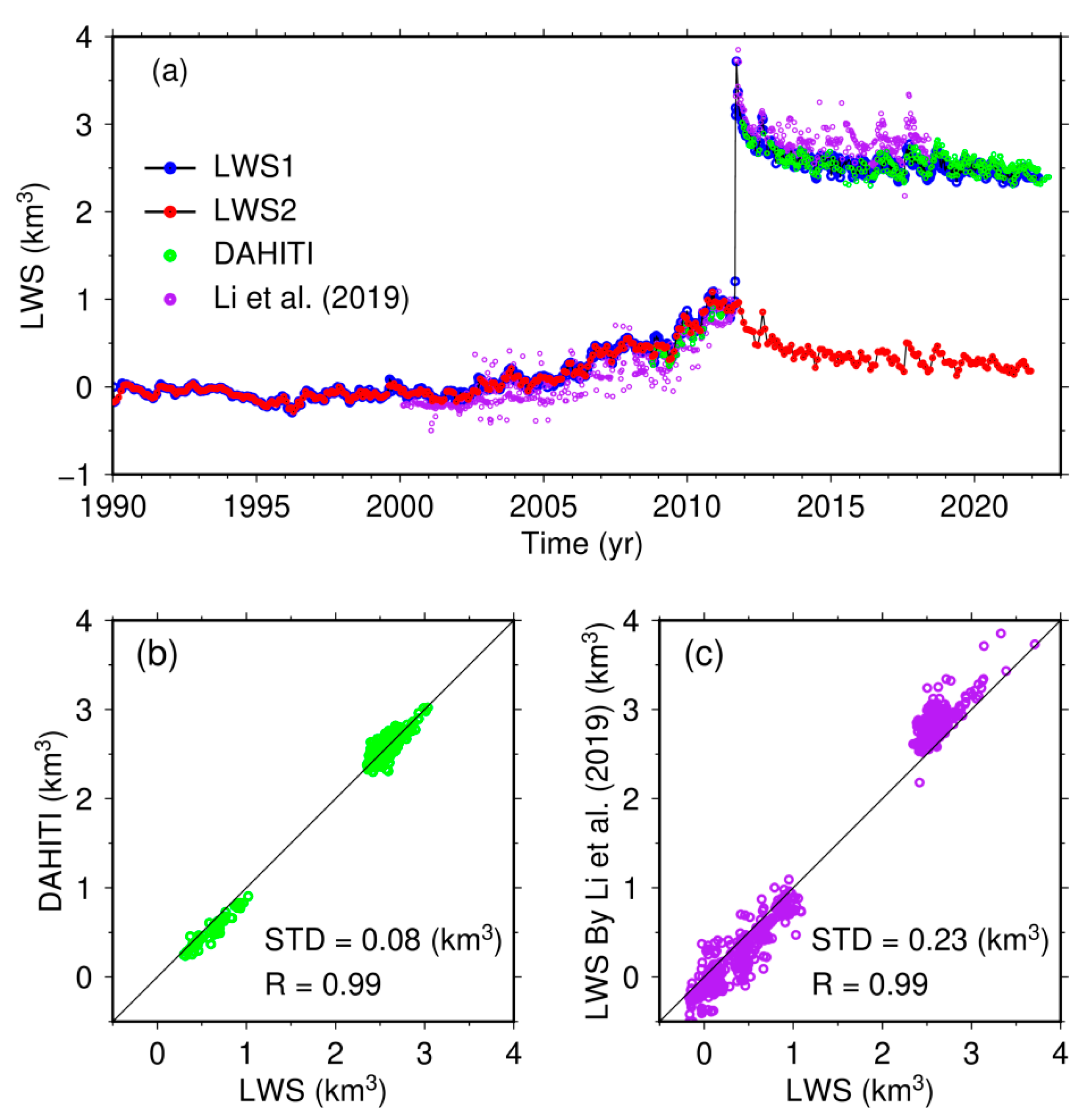
4.3. The LWS Time Series of the KL
5. Discussion
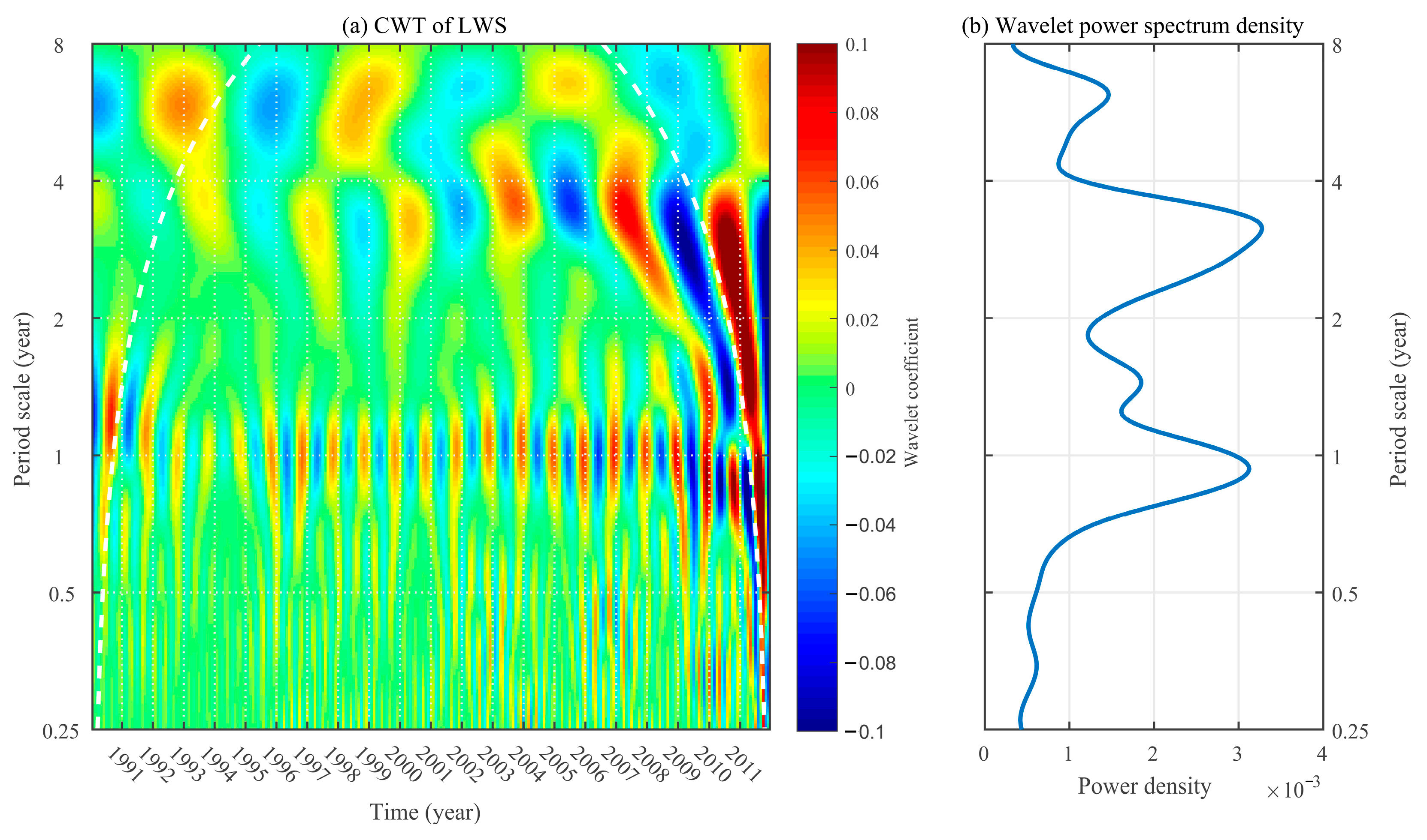
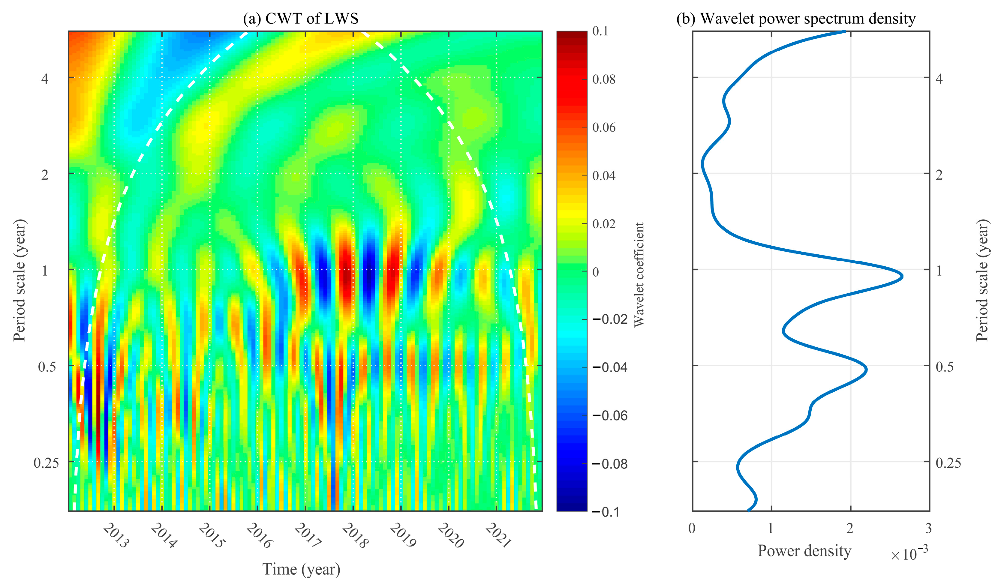
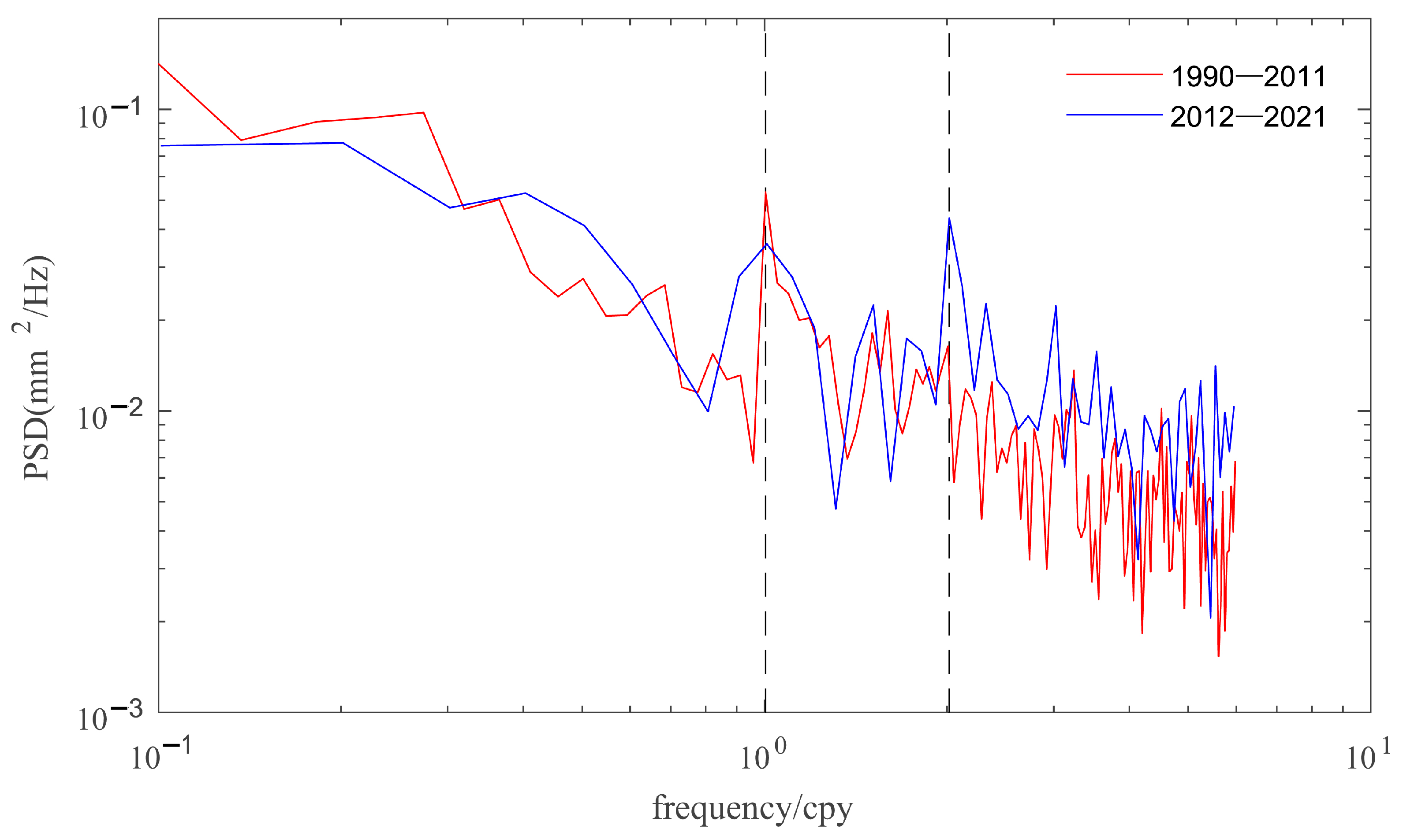
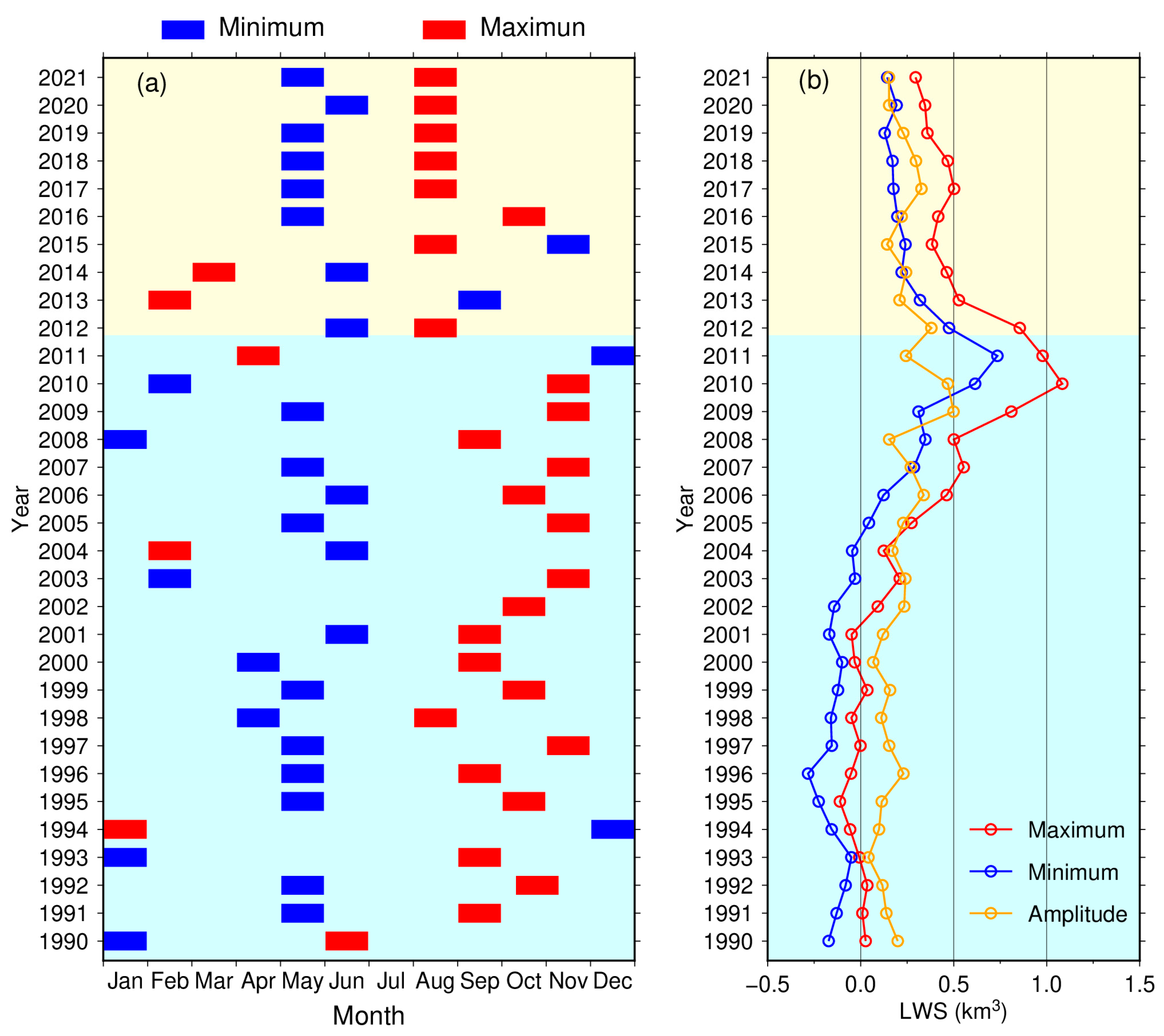
5.1. Periodic Variations of the LWS of KL before and after the Outburst
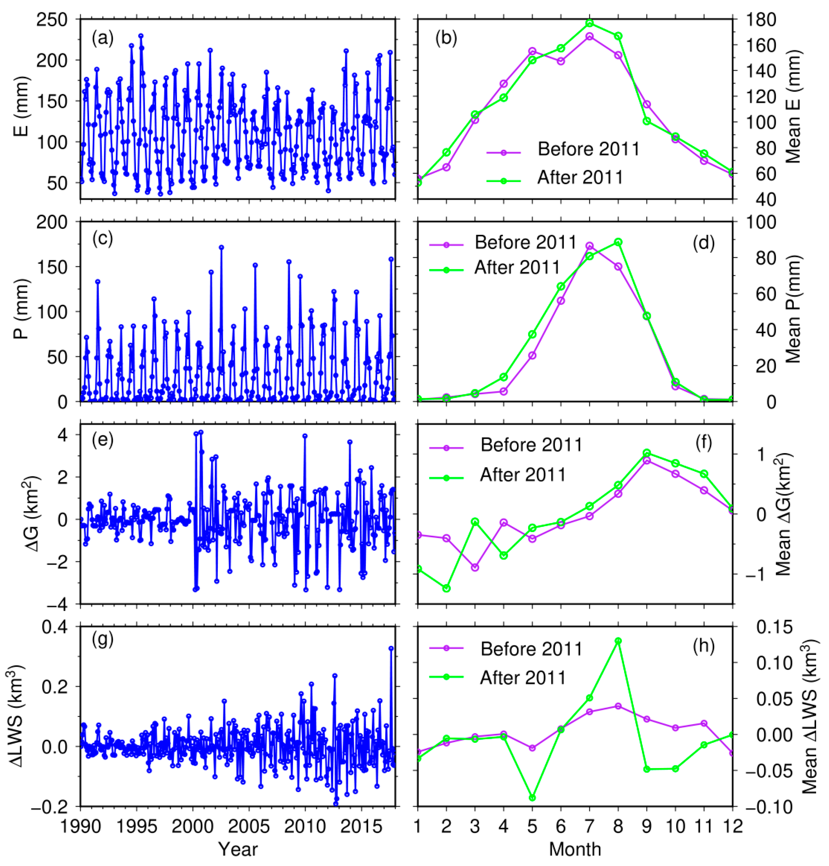
5.2. Annual LWS Variations before and after the Outburst
5.3. Possible Driving Factors of Pattern Change in the TWS Variation
6. Conclusions
Author Contributions
Funding
Data Availability Statement
Acknowledgments
Conflicts of Interest
References
- Yang, K.; Lu, H.; Yue, S.; Zhang, G.Q.; Lei, Y.B.; La, Z.; Wang, W. Quantifying recent precipitation change and predicting lake expansion in the Inner Tibetan Plateau. Clim. Chang. 2018, 147, 149–163. [Google Scholar] [CrossRef]
- Zhang, G.Q.; Yao, T.D.; Shum, C.K.; Yi, S.; Yang, K.; Xie, H.J.; Feng, W.; Bolch, T.; Wang, L.; Behrangi, A.; et al. Lake volume and groundwater storage variations in Tibetan Plateau’s endorheic basin. Geophys. Res. Lett. 2017, 44, 5550–5560. [Google Scholar] [CrossRef]
- Zhang, X.L.; Xu, B.Q.; Xie, Y.; Li, J.L.; Li, Y.N. Continuous mass loss acceleration of Qiangyong Glacier, southern Tibetan plateau, since the mid-1880s inferred from glaciolacustrine sediments. Quat. Sci. Rev. 2017, 301, 107937. [Google Scholar] [CrossRef]
- Lei, Y.B.; Yang, K. The cause of rapid lake expansion in the Tibetan Plateau: Climate wetting or warming? Wiley Interdiscip. Rev. Water 2017, 4, e1236. [Google Scholar] [CrossRef]
- Liu, W.H.; Xie, C.W.; Zhao, L.; Li, R.; Liu, G.Y.; Wang, W.; Liu, H.R.; Wu, T.H.; Yang, G.Q.; Zhang, Y.X.; et al. Rapid expansion of lakes in the endorheic basin on the Qinghai-Tibet Plateau since 2000 and its potential drivers. Catena 2021, 197, 104942. [Google Scholar] [CrossRef]
- Huang, Z.K. Lake Water Storage Changes over the Qinghai-Tibetan Plateau from Multi-Mission Satellite Data and Its Influencing Factors Analysis. Ph.D. Thesis, Wuhan University, Wuhan, China, 2018. [Google Scholar]
- Liu, B.K.; Du, Y.E.; Li, L.; Feng, Q.S.; Xie, H.J.; Liang, T.G.; Hou, F.J.; Ren, J.Z. Outburst flooding of the moraine-dammed Zhuonai Lake on Tibetan plateau: Causes and impacts. IEEE Geosci. Remote Sens. Lett. 2016, 13, 570–574. [Google Scholar] [CrossRef]
- Liu, K.; Ke, L.H.; Wang, J.D.; Jiang, L.; Richards, K.S.; Sheng, Y.W.; Zhu, Y.Q.; Fan, C.Y.; Zhan, P.F.; Luo, S.X.; et al. Ongoing drainage reorganization driven by rapid lake growths on the Tibetan Plateau. Geophys. Res. Lett. 2021, 48, e2021GL095795. [Google Scholar] [CrossRef]
- Lu, S.L.; Jin, J.M.; Zhou, J.F.; Li, X.D.; Ju, J.T.; Li, M.Y.; Chen, F.; Zhu, L.P.; Zhao, H.L.; Yan, Q.; et al. Drainage basin reorganization and endorheic-exorheic transition triggered by climate change and human intervention. Glob. Planet. Chang. 2021, 201, 103494. [Google Scholar] [CrossRef]
- Liu, W.H.; Xie, C.W.; Zhao, L.; Wu, T.H.; Wang, W.; Zhang, Y.X.; Yang, G.Q.; Zhu, X.F.; Yue, G.Y. Dynamic changes in lakes in the Hoh Xil region before and after the 2011 outburst of Zonag Lake. J. Mt. Sci. 2019, 16, 1098–1110. [Google Scholar] [CrossRef]
- Lu, P.; Han, J.P.; Li, Z.S.; Xu, R.G.; Li, R.X.; Hao, T.; Qiao, G. Lake outburst accelerated permafrost degradation on Qinghai-Tibet Plateau. Remote Sens. Environ. 2020, 249, 112011. [Google Scholar] [CrossRef]
- Fu, C.C.; Li, X.Q.; Cheng, X. Unraveling the mechanisms underlying lake expansion from 2001 to 2020 and its impact on the ecological environment in a typical alpine basin on the Tibetan Plateau. China Geol. 2023, 6, 216–227. [Google Scholar] [CrossRef]
- Yao, X.J.; Liu, S.Y.; Sun, M.P.; Guo, W.Q.; Zhang, X. Changes of Kusai Lake in Hoh Xil Region and Causes of Its Water Overflowing. Acta Geogr. Sin. 2012, 67, 689–698. [Google Scholar]
- Hu, Z.K.; Tan, D.B.; Wen, X.F.; Chen, B.Q.; Shen, D.T. Investigation of dynamic lake changes in Zhuonai Lake—Salt Lake Basin, Hoh Xil, using remote sensing images in response to climate change (1989–2018). J. Water Clim. Chang. 2021, 12, 2199–2216. [Google Scholar] [CrossRef]
- Hwang, C.W.; Cheng, Y.S.; Han, J.; Kao, R.; Huang, C.Y.; Wei, S.H.; Wang, H. Multi-Decadal Monitoring of Lake Level Changes in the Qinghai-Tibet Plateau by the TOPEX/Poseidon-Family Altimeters: Climate Implication. Remote Sens. 2016, 8, 446. [Google Scholar] [CrossRef]
- Guo, H.; Nie, B.; Yuan, Y.; Yang, H.; Dai, W.; Wang, X.; Qiao, B. Continuous Intra-Annual Changes of Lake Water Level and Water Storage from 2000 to 2018 on the Tibetan Plateau. Remote Sens. 2023, 15, 893. [Google Scholar] [CrossRef]
- Hwang, C.W.; Cheng, Y.S.; Yang, W.H.; Zhang, G.Q.; Huang, Y.R.; Shen, W.B.; Pan, Y.J. Lake level changes in the Tibetan Plateau from Cryosat-2, SARAL, ICESat, and Jason-2 altimeters. Terr. Atmos. Ocean. Sci. 2019, 30, 33–50. [Google Scholar] [CrossRef]
- Li, X.D.; Long, D.; Han, P.F.; Zhao, F.Y.; Wada, Y. Densified multi-mission observations by developed optical water levels show marked increases in lake water storage and overflow floods on the Tibetan Plateau. Earth Syst. Sci. Data Discuss. 2019, 2, 1–34. [Google Scholar]
- Hwang, C.W.; Peng, M.F.; Ning, J.S.; Luo, J.; Sui, C.H. Lake level variations in China from TOPEX/Poseidon altimetry: Data quality assessment and links to precipitation and ENSO. Geophy. J. Int. 2005, 161, 1–11. [Google Scholar] [CrossRef]
- Wang, H.H.; Chu, Y.H.; Huang, Z.K.; Hwang, C.W.; Chao, N.F. Robust, long-term lake level change from multiple satellite altimeters in Tibet: Observing the rapid rise of Ngangzi Co over a new wetland. Remote Sens. 2019, 11, 558. [Google Scholar] [CrossRef]
- Zhang, G.Q.; Xie, H.J.; Kang, S.C.; Yi, D.H.; Ackley, S.F. Monitoring lake level changes on the Tibetan Plateau using ICESat altimetry data (2003–2009). Remote Sens. Environ. 2011, 115, 1733–1742. [Google Scholar] [CrossRef]
- Fernandes, M.J.; Lázaro, C.; Nunes, A.L.; Scharroo, R. Atmospheric Corrections for Altimetry Studies over Inland Water. Remote Sens. 2014, 6, 4952–4997. [Google Scholar] [CrossRef]
- Vieira, T.; Fernandes, M.J.; Lazaro, C. Analysis and retrieval of tropospheric corrections for CryoSat-2 over inland waters. Adv. Space Res. 2018, 62, 1479–1496. [Google Scholar] [CrossRef]
- Tseng, K.H.; Shum, C.K.; Yi, Y.; Emery, W.J.; Kuo, C.Y.; Lee, H.; Wang, H. The improved retrieval of coastal sea surface heights by retracking modified radar altimetry waveforms. IEEE Trans. Geosci. Remote Sens. 2013, 52, 991–1001. [Google Scholar] [CrossRef]
- Huang, Z.K.; Wang, H.H.; Luo, Z.C.; Shum, C.K.; Tseng, K.H.; Zhong, B. Improving Jason-2 Sea Surface Heights within 10 km Offshore by Retracking Decontaminated Waveforms. Remote Sens. 2017, 9, 1077. [Google Scholar] [CrossRef]
- Wang, H.H.; Huang, Z.K. Waveform decontamination for improving satellite radar altimeter data over nearshore area: Upgraded algorithm and validation. Front. Earth Sci. 2021, 9, 748401. [Google Scholar] [CrossRef]
- Bai, T.; Li, D.R.; Sun, K.M.; Chen, Y.P.; Li, W.Z. Cloud detection for high-resolution satellite imagery using machine learning and multi-feature fusion. Remote Sens. 2016, 8, 715. [Google Scholar] [CrossRef]
- Gu, L.J.; Ren, R.Z.; Zhang, S. Automatic Cloud Detection and Removal Algorithm for MODIS Remote Sensing Imagery. J. Soft. 2011, 6, 1289–1296. [Google Scholar] [CrossRef]
- Xie, F.Y.; Shi, M.Y.; Shi, Z.W.; Yin, J.H.; Zhao, D.P. Multilevel cloud detection in remote sensing images based on deep learning. IEEE J. Sel. Top. Appl. Earth Obs. Remote Sens. 2017, 10, 3631–3640. [Google Scholar] [CrossRef]
- Song, C.Q.; Huang, B.; Ke, L.H.; Richards, K.S. Remote sensing of alpine lake water environment changes on the Tibetan Plateau and surroundings: A review. ISPRS J. Photogramm. Remote Sens. 2014, 92, 26–37. [Google Scholar] [CrossRef]
- Wang, X.R.; Jin, R.; Lin, J.; Zeng, X.F.; Zhao, Z.B. Automatic Algorithm for Extracting Lake Boundaries in Qinghai-Tibet Plateau based on Cloudy Landsat TM/OLI Image and DEM. Remote Sens. Technol. Appl. 2020, 35, 882–892. [Google Scholar]
- Xiong, J.H.; Jiang, L.G.; Qiu, Y.L.; Wongchuig, S.; Guo, S.L.; Chen, J. On the capabilities of the SWOT satellite to monitor the lake level change over the Thrid Pole. Environ. Res. Lett. 2023, 18, 044008. [Google Scholar] [CrossRef]
- Li, X.D.; Long, D.; Huang, Q.; Han, P.; Zhao, F.; Wada, Y. High-temporal-resolution water level and storage change data sets for lakes on the Tibetan Plateau during 2000–2017 using multiple altimetric missions and Landsat-derived lake shoreline positions. Earth Syst. Sci. Data 2019, 11, 1603–1627. [Google Scholar] [CrossRef]
- Wang, H.H.; Huang, Z.K.; Wen, Z.Q.; Luo, Z.C. Lake Water Storage Changes in Northeast Hoh Xil Observed by Cryosat-2 and Landsat-5/7/8: Impact of the Outburst of Zhuonai Lake in 2011. IEEE Geosci. Remote Sens. Lett. 2022, 19, 1504205. [Google Scholar] [CrossRef]
- Cui, A.N.; Lu, H.Y.; Liu, X.Q.; Shen, C.M.; Xu, D.K.; Xu, B.Q.; Wu, N.Q. Tibetan plateau precipitation modulated by the periodically coupled westerlies and Asian monsoon. Geophys. Res. Lett. 2021, 48, e2020GL091543. [Google Scholar] [CrossRef]
- Jiang, L.G.; Nielsen, K.; Andersen, O.B.; Bauer-Gottwein, P. A bigger picture of how the Tibetan lakes have changed over the past decade revealed by CryoSat-2 altimetry. J. Geophys. Res. Atmos. 2020, 125, e2020JD033161. [Google Scholar] [CrossRef]
- Wan, J.; Liao, J.J.; Xu, T.; Shen, G.Z. Accuracy evaluation of SRTM data based on ICESat/GLAS altimeter data: A case study in the Tibetan Plateau. Remote Sens. Land Resour. 2015, 27, 100–105. [Google Scholar]
- Cowan, D.; Cooper, G. The Shuttle Radar Topography Mission-a new source of near-global digital elevation data. Explor. Geophys. 2005, 36, 334–340. [Google Scholar] [CrossRef]
- Zhang, J.; Hu, Q.W.; Li, Y.K.; Li, H.D.; Li, J.Y. Area, lake-level and volume variations of typical lakes on the Tibetan Plateau and their response to climate change, 1972–2019. Geo-Spat. Inf. Sci. 2021, 24, 458–473. [Google Scholar] [CrossRef]
- Liu, X.Q.; Yu, Z.T.; Dong, H.L.; Chen, H.F. A less or more dusty future in the Northern Qinghai-Tibetan Plateau? Sci. Rep. 2014, 4, 6672. [Google Scholar] [CrossRef]
- McFeeters, S.K. The use of the Normalized Difference Water Index (NDWI) in the delineation of open water features. Int. J. Remote Sens. 1996, 17, 1425–1432. [Google Scholar] [CrossRef]
- Li, X.; Zhang, F.; Chan, N.W.; Shi, J.; Liu, C.; Chen, D. High Precision Extraction of Surface Water from Complex Terrain in Bosten Lake Basin Based on Water Index and Slope Mask Data. Water 2022, 14, 2809. [Google Scholar] [CrossRef]
- Bolch, T.; Peters, J.; Yegorov, A.; Pardhan, B.; Buchroithner, M.; Blagoveshchensky, V. Identification of potentially dangerous glacial lakes in the northern Tien Shan. Nat. Hazards 2011, 59, 1691–1714. [Google Scholar] [CrossRef]
- Yang, Y.D.; Moore, P.; Li, Z.H.; Li, F. Lake level change from satellite altimetry over seasonally ice-covered lakes in the Mackenzie River basin. IEEE Trans. Geosci. Remote Sens. 2020, 59, 8143–8152. [Google Scholar] [CrossRef]
- Sun, M.; Guo, J.; Yuan, J.; Liu, X.; Wang, H.; Li, C. Detecting Lake Level Change from 1992 to 2019 of Zhari Namco in Tibet Using Altimetry Data of TOPEX/Poseidon and Jason-1/2/3 Missions. Front. Earth Sci. 2021, 9, 640553. [Google Scholar] [CrossRef]
- Hersbach, H.; Bell, B.; Berrisford, P.; Biavati, G.; Horányi, A.; Muñoz Sabater, J.; Nicolas, J.; Peubey, C.; Radu, R.; Rozum, I.; et al. ERA5 Hourly Data on Single Levels from 1940 to Present. Copernicus Climate Change Service (C3S) Climate Data Store (CDS). 2018. Available online: https://cds.climate.copernicus.eu/cdsapp#!/dataset/reanalysis-era5-single-levels?tab=overview (accessed on 10 May 2022).
- Zhang, Y.J.; Wang, N.L.; Yang, X.W.; Mao, Z.L. The Dynamic Changes of Lake Issyk-Kul from 1958 to 2020 Based on Multi-Ssource Satellite Data. Remote Sens. 2022, 14, 1575. [Google Scholar] [CrossRef]
- Zhan, P.F.; Liu, K.; Zhang, Y.C.; Ma, R.H.; Song, C.Q. A Comparative Study on the Changes of Typical Lakes in Different Climate Zones of the Tibetan Plateau at Multi-Timescales based on Remote Sensing Observations. Remote Sens. Technol. Appl. 2021, 36, 90–102. [Google Scholar]
- Zhang, G.Q.; Yao, T.D.; Xie, H.J.; Yang, K.; Zhu, L.P.; Shum, C.K.; Bolch, T.; Yi, S.; Allen, S.; Jiang, L.G.; et al. Response of Tibetan Plateau lakes to climate change: Trends, patterns, and mechanisms. Earth Sci. Rev. 2020, 208, 103269. [Google Scholar] [CrossRef]
- Liao, J.J.; Shen, G.Z.; Zhao, Y. Dataset of Global Lake Level Changes Using Multi-Altimeter Data (2002–2016). J. Glob. Chang. Data Discov. 2018, 2, 295–302. [Google Scholar]
- Schwatke, C.; Dettmering, D.; Bosch, W.; Seitz, F. DAHITI—An innovative approach for estimating water level time series over inland waters using multi-mission satellite altimetry. Hydrol. Earth Syst. Sci. 2015, 19, 4345–4364. [Google Scholar] [CrossRef]
- Shu, S.; Liu, H.X.; Beck, R.A.; Frappart, F.; Korhonen, J.; Lan, M.X.; Yang, B.; Huang, Y. Evaluation of historic and operational satellite radar altimetry missions for constructing consistent long-term lake water level records. Hydrol. Earth Syst. Sci. 2021, 25, 1643–1670. [Google Scholar] [CrossRef]
- Yao, X.J.; Liu, S.Y.; Li, L.; Sun, M.P.; Luo, J. Spatial-temporal characteristics of lake area variations in Hoh Xil region from 1970 to 2011. J. Geogr. Sci. 2014, 24, 689–702. [Google Scholar] [CrossRef]
- Guo, J.Y.; Li, W.; Liu, X.; Kong, Q.L.; Zhao, C.M.; Guo, B. Temporal-Spatial Variation of Global GPS-Derived Total Electron Content, 1999–2013. PLoS ONE 2015, 10, e0133378. [Google Scholar] [CrossRef] [PubMed]
- Welch, P. The use of fast Fourier transform for the estimation of power spectra: A method based on time averaging over short, modified periodograms. IEEE Trans. Audio Electr. 1967, 15, 70–73. [Google Scholar] [CrossRef]
- He, X.X.; Hua, X.H.; Yu, K.G.; Xuan, W.; Lu, T.D.; Zhang, W.; Chen, X.J. Accuracy enhancement of GPS time series using principal component analysis and block spatial filtering. Adv. Space Res. 2015, 55, 1316–1327. [Google Scholar] [CrossRef]
- Li, L.; Tan, D.B.; Wen, X.F.; Wang, Y.; Liu, X.S.; Wang, G. Impact of Climate Change on the Change of Lake Water Volume in the Hoh Xil Salt Lake Basin. J. Yangtze River Sci. Res. Inst. 2022, 39, 16–23. [Google Scholar]


| Satellite | Altimeter | Along-Track Resolution (20 Hz) | Repeat Cycle | Time Span | Available Cycles |
|---|---|---|---|---|---|
| ERS-2 | RA-1 | 330 m | 35 d | May 1995–February 2003 | 78 |
| Jason-1 | Poseidon-2 | 290 m | 9.91 d | February 2002–April 2011 | 100 |
| Jason-2 | Poseidon-3 | 290 m | 9.91 d | October 2008–May 2017 | 186 |
| Jason-3 | Poseidon-3B | 290 m | 9.91 d | March 2016–April 2022 | 208 |
| Satellite | Spatial Resolution | Repeat Cycle | Band | Time Span | No. of Images |
|---|---|---|---|---|---|
| Landsat-5 | 30 m | 16 d | Green\NIR(Band2\Band4) | January 1990–October 2011 | 275 |
| Landsat-7 | 30 m | 16 d | Green\NIR(Band2\Band4) | September 1999–August 2021 | 275 |
| Landsat-8 | 30 m | 16 d | Green\NIR(Band3\Band5) | May 2013–November 2021 | 134 |
| Literature | Dataset | Data Source | Time Range | Density of Data |
|---|---|---|---|---|
| This study | Level/Area/LWS | ERS-2, Jason-1/2/3, Landsat-5/7/8 | January 1990–December 2021 | 35.7/y |
| Liao et al. (2018) [50] | Level/-/- | Envisat, Jason-2, Cryosat-2 | August 2002–January 2017 | 10.6/y |
| DAHITI [51] | Level/-/- | Jason-2/3, Saral, Sentinel-3A | October 2008–August 2022 | 27.6/y |
| Li et al. (2019) [33] | Level/-/LWS | Envisat, Jason-1/2/3, ICESat, Cryosat-2 | February 2000–June 2018 | 38.8/y |
| No. of Samples | Average Interval | Min Interval | Max Interval | |
|---|---|---|---|---|
| Landsat-derived area | 582 | 16.49 d | 1 d | 153 d (26 May 2012–26 October 2012) |
| Altimeter-derived level | 469 | 20.47 d | 2.38 d | 175 d (8 January 2001–2 July 2001) |
| LWS | 1051 | 9.13 d | 1 d | 65 d (11 August 2008–15 October 2008) |
Disclaimer/Publisher’s Note: The statements, opinions and data contained in all publications are solely those of the individual author(s) and contributor(s) and not of MDPI and/or the editor(s). MDPI and/or the editor(s) disclaim responsibility for any injury to people or property resulting from any ideas, methods, instructions or products referred to in the content. |
© 2023 by the authors. Licensee MDPI, Basel, Switzerland. This article is an open access article distributed under the terms and conditions of the Creative Commons Attribution (CC BY) license (https://creativecommons.org/licenses/by/4.0/).
Share and Cite
Huang, Z.; Wu, X.; Wang, H.; Zhao, Z.; Du, L.; He, X.; Zhou, H. Characterizing the Water Storage Variation of Kusai Lake by Constructing Time Series from Multisource Remote Sensing Data. Remote Sens. 2024, 16, 128. https://doi.org/10.3390/rs16010128
Huang Z, Wu X, Wang H, Zhao Z, Du L, He X, Zhou H. Characterizing the Water Storage Variation of Kusai Lake by Constructing Time Series from Multisource Remote Sensing Data. Remote Sensing. 2024; 16(1):128. https://doi.org/10.3390/rs16010128
Chicago/Turabian StyleHuang, Zhengkai, Xin Wu, Haihong Wang, Zehui Zhao, Liting Du, Xiaoxing He, and Hangyu Zhou. 2024. "Characterizing the Water Storage Variation of Kusai Lake by Constructing Time Series from Multisource Remote Sensing Data" Remote Sensing 16, no. 1: 128. https://doi.org/10.3390/rs16010128
APA StyleHuang, Z., Wu, X., Wang, H., Zhao, Z., Du, L., He, X., & Zhou, H. (2024). Characterizing the Water Storage Variation of Kusai Lake by Constructing Time Series from Multisource Remote Sensing Data. Remote Sensing, 16(1), 128. https://doi.org/10.3390/rs16010128