
A Method for Detecting Ionospheric TEC Anomalies before Earthquake: The Case Study of Ms 7.8 Earthquake, February 06, 2023, Türkiye


Abstract
:1. Introduction
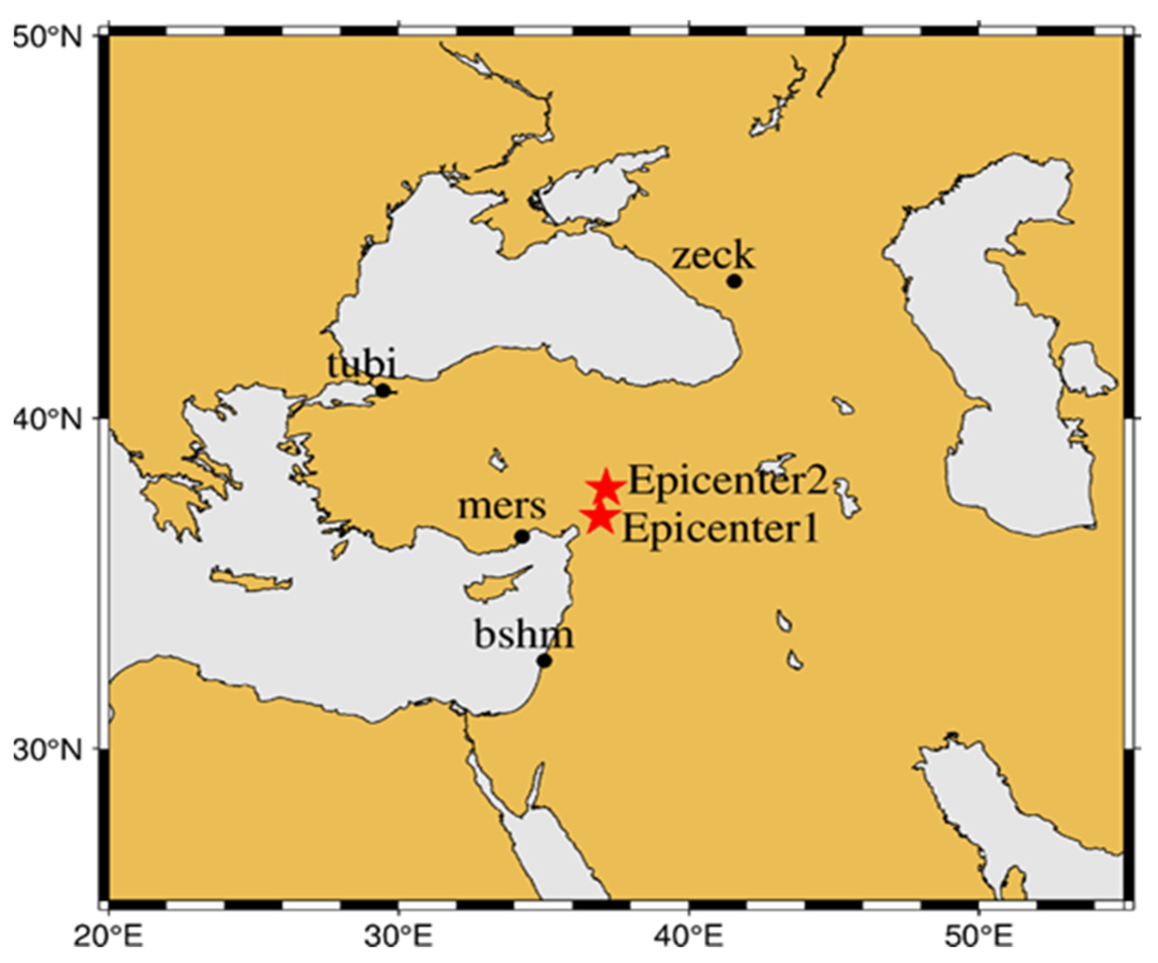
2. Data Sources
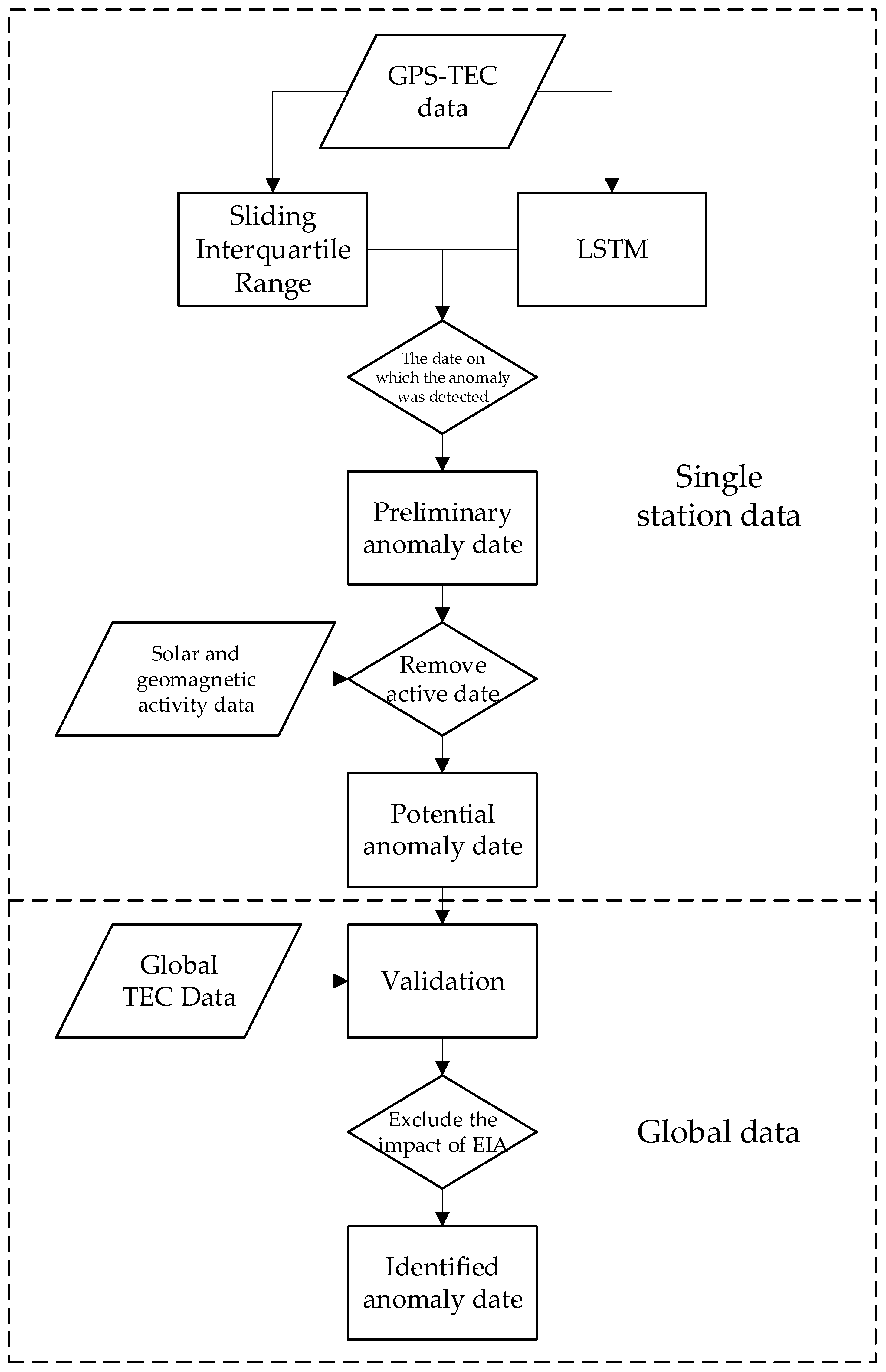
3. Method
4. Result Analysis and Discussion
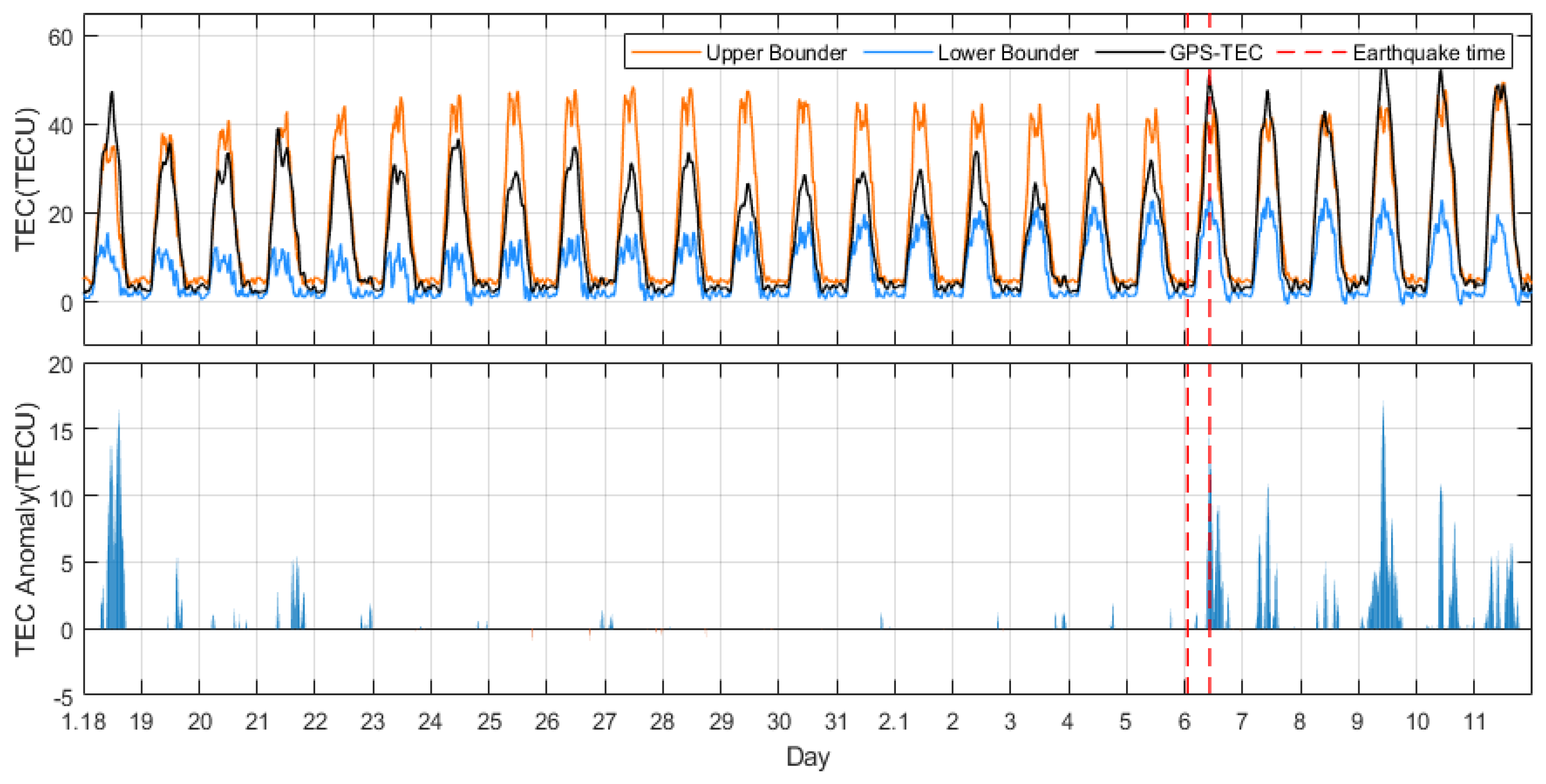
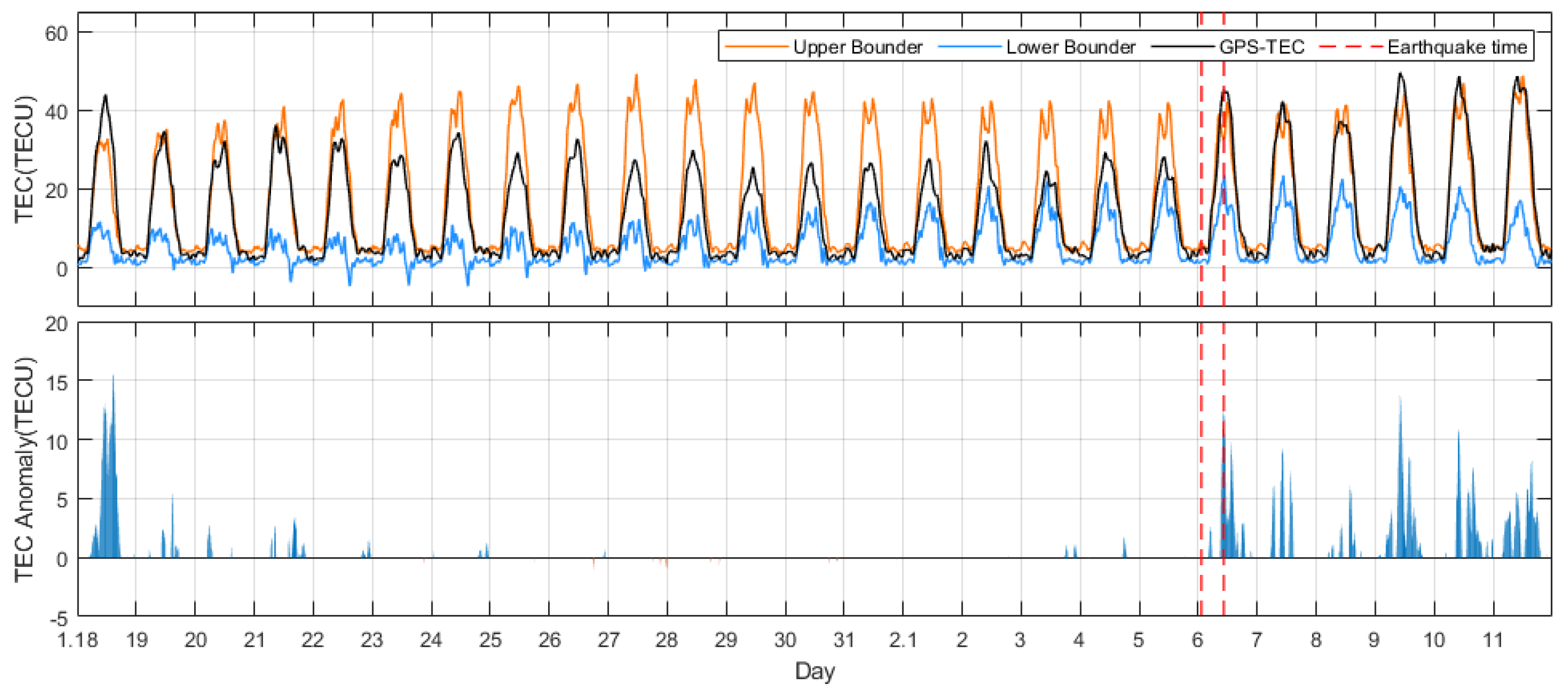
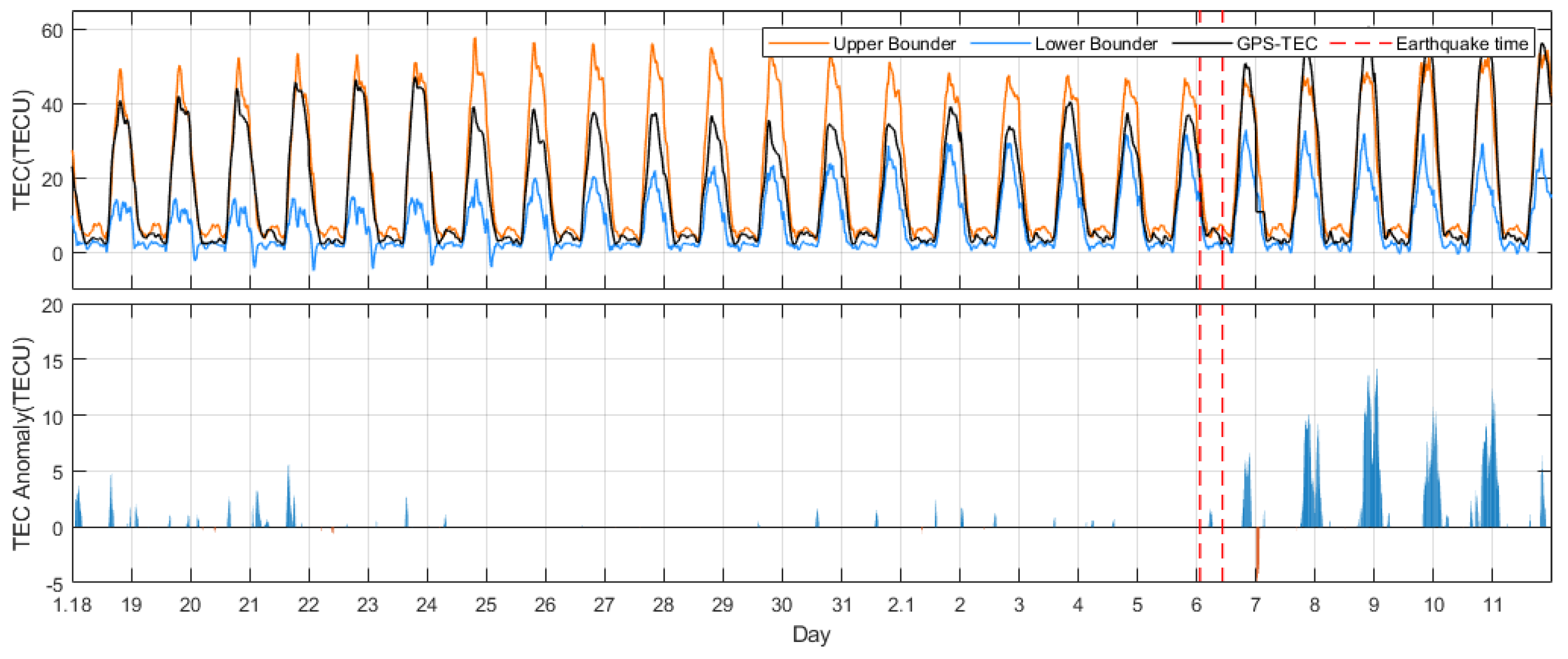
4.1. Sliding Interquartile Range Method Was Used to Analyze TEC Anomalies in a Single Station
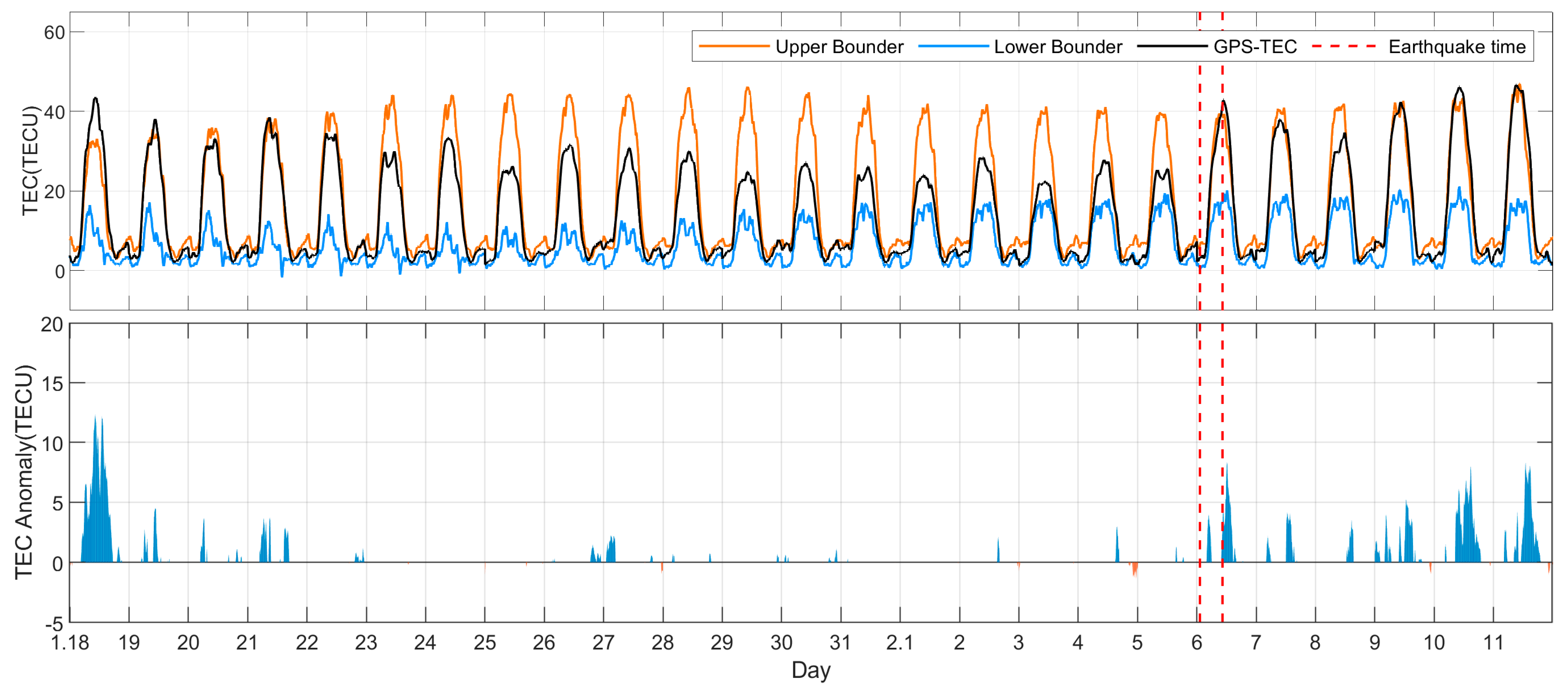
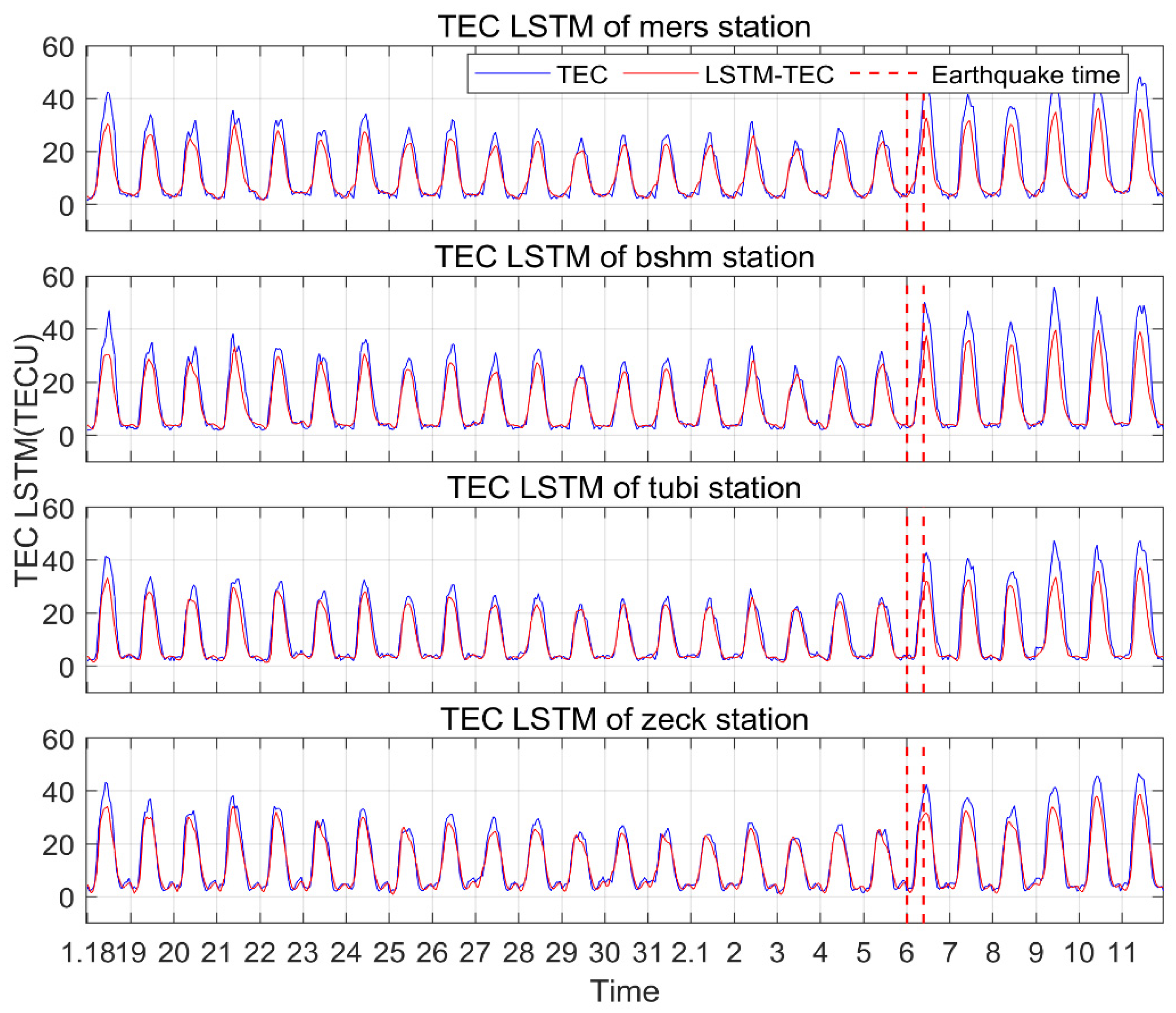
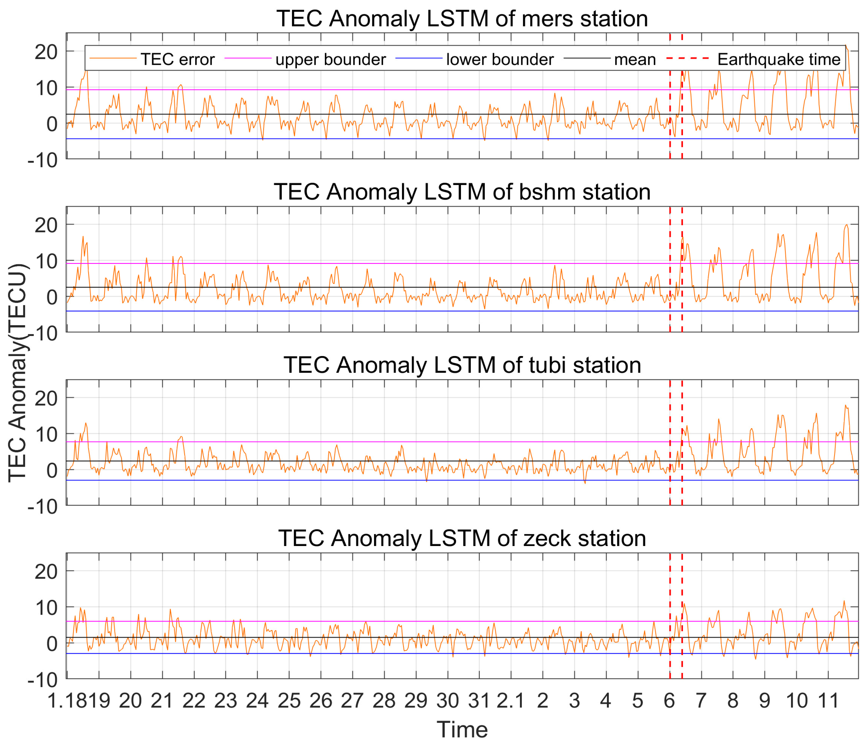
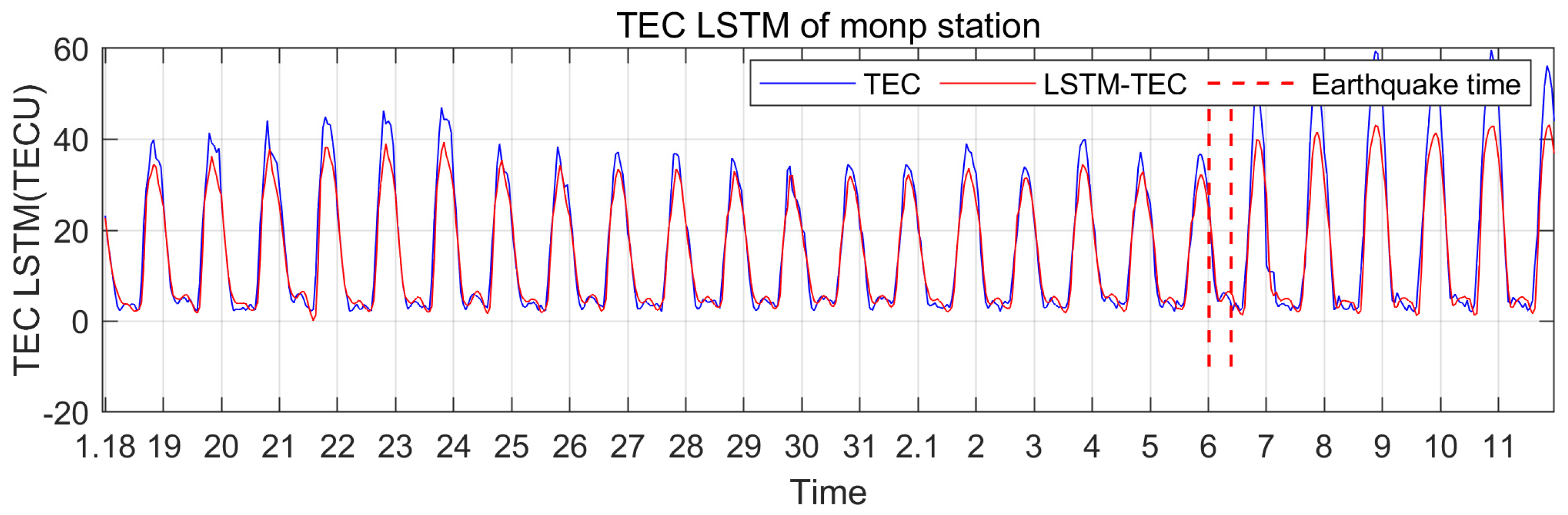
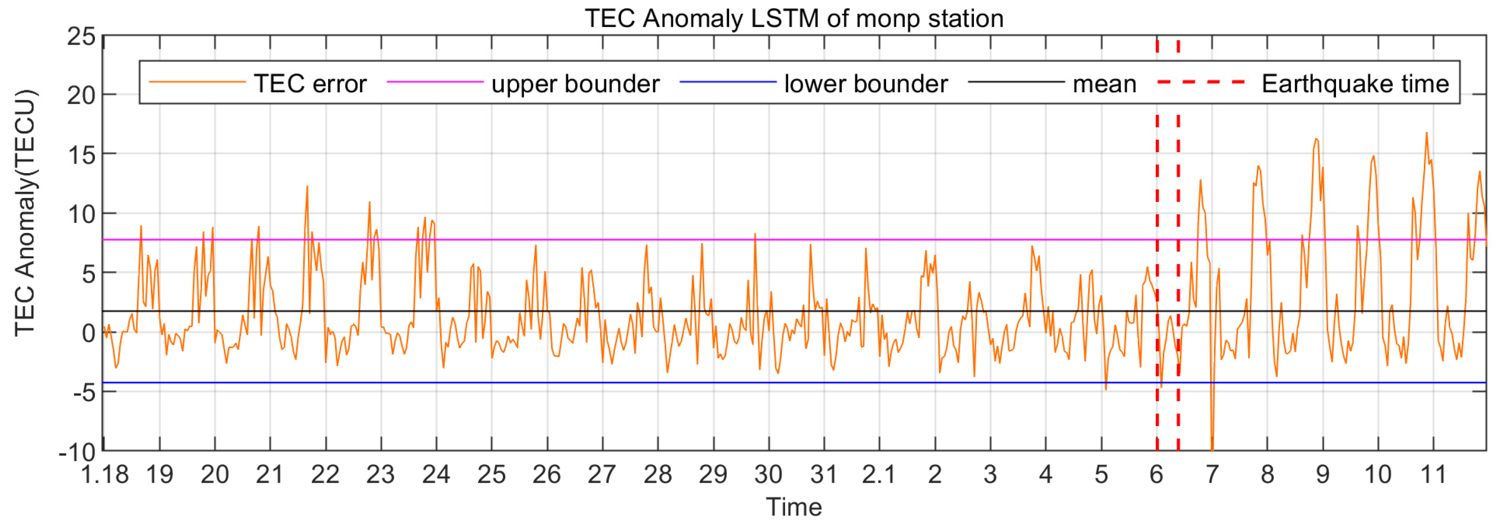
4.2. LSTM Was Used to Analyze Single-Station TEC Anomalies
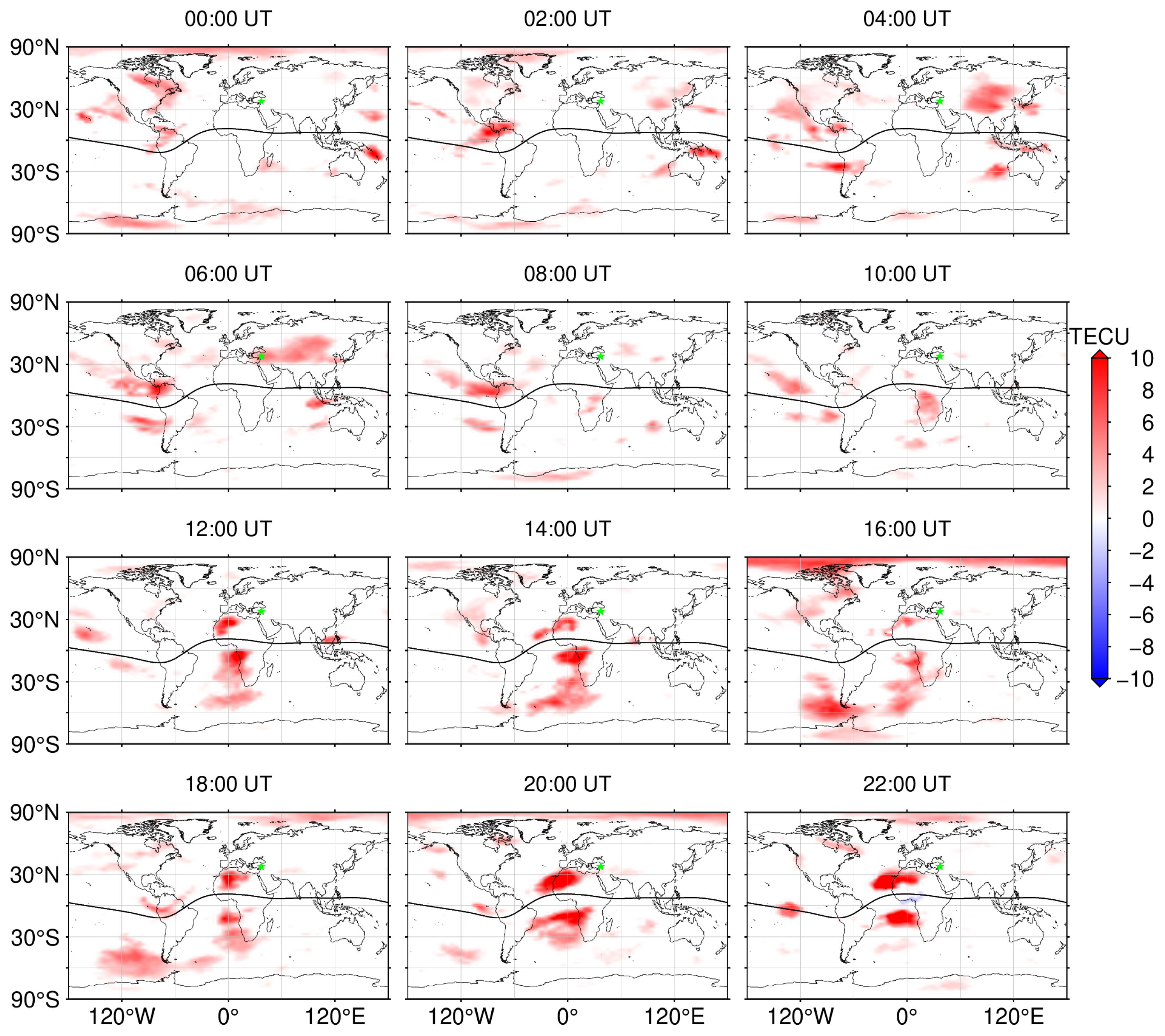
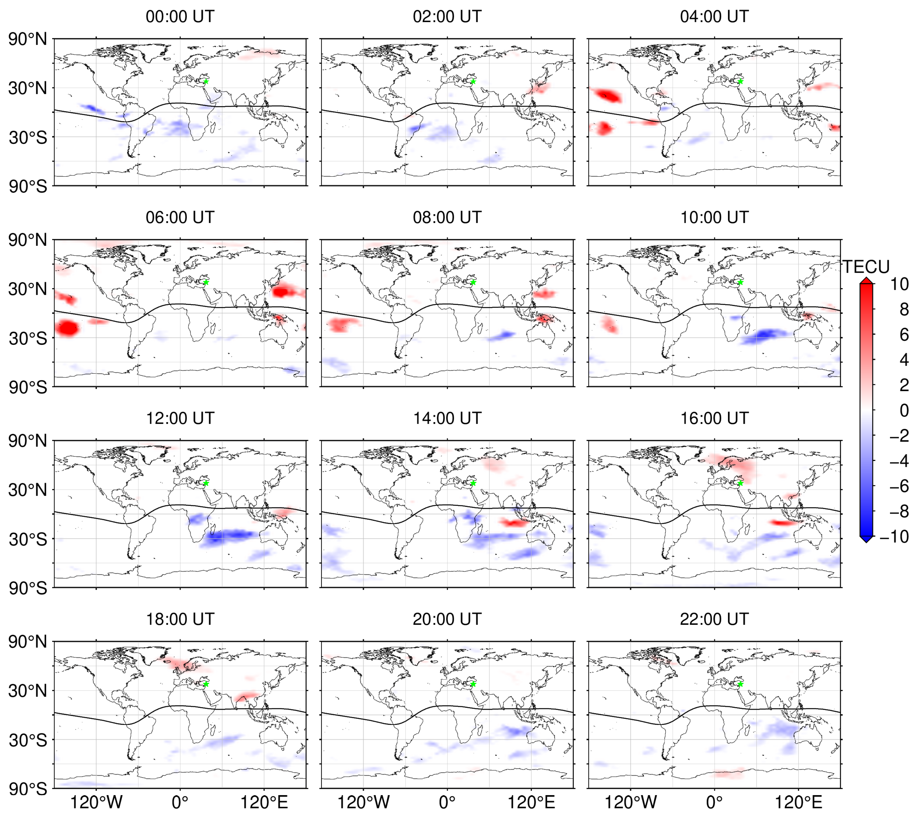
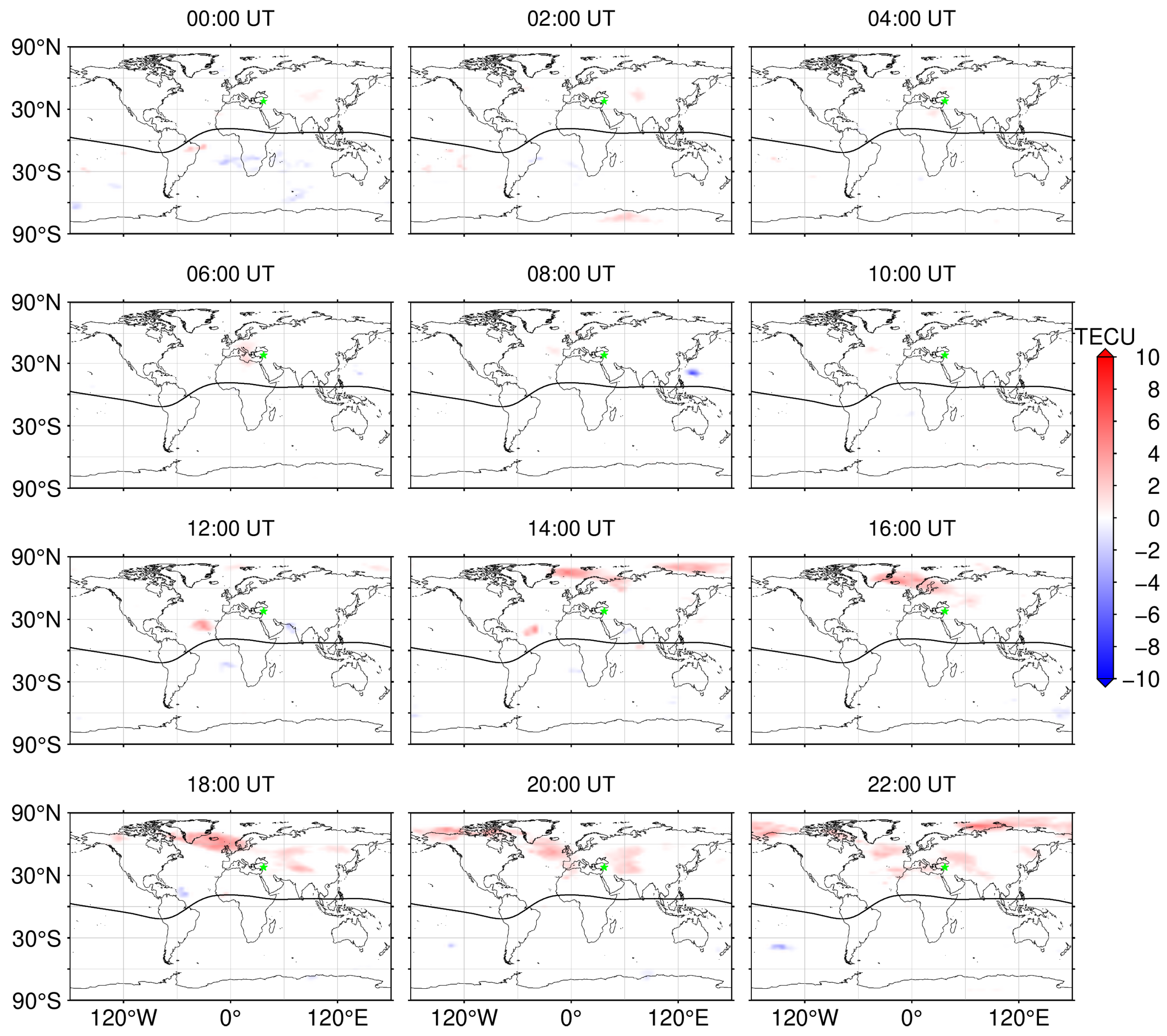
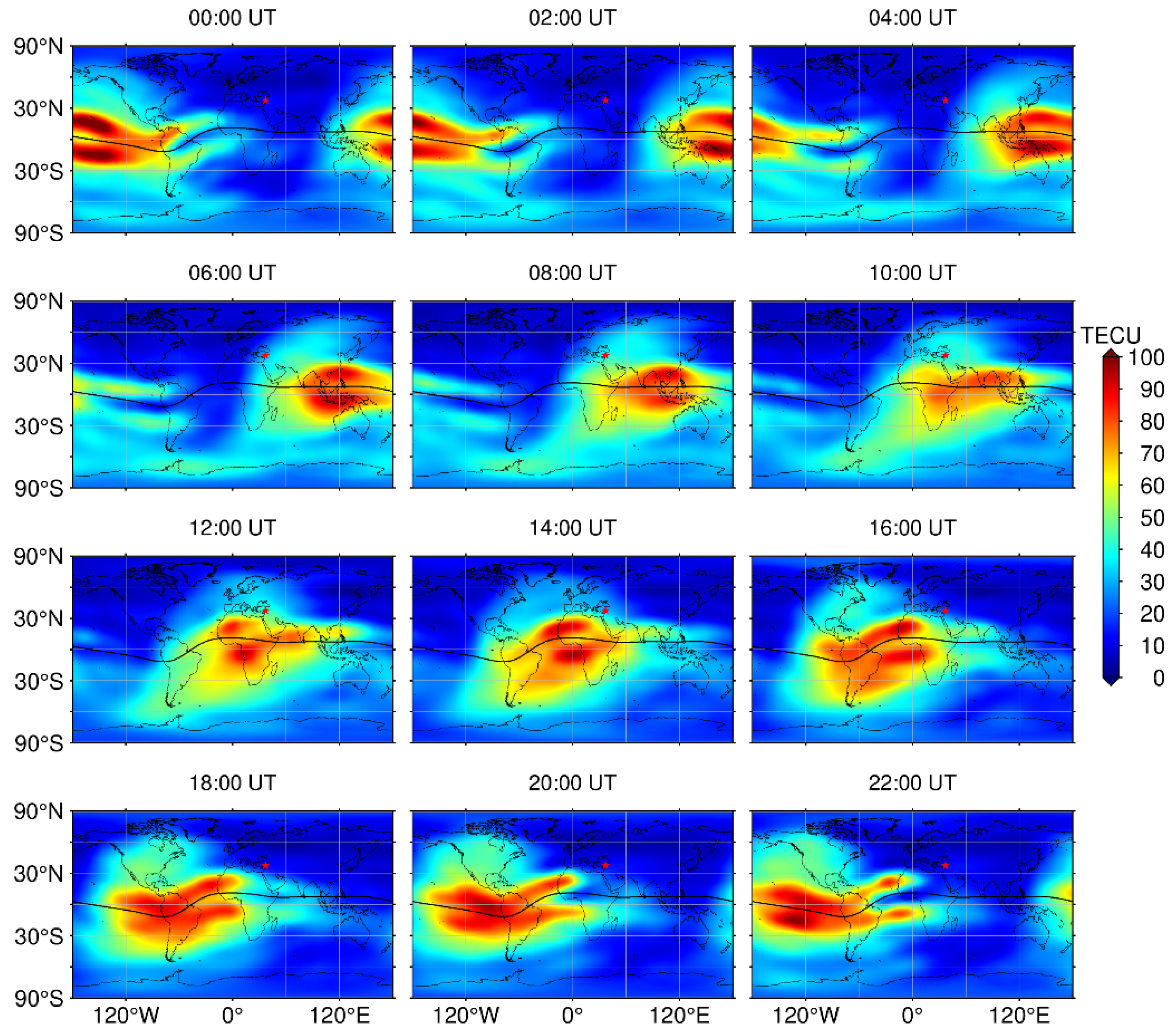
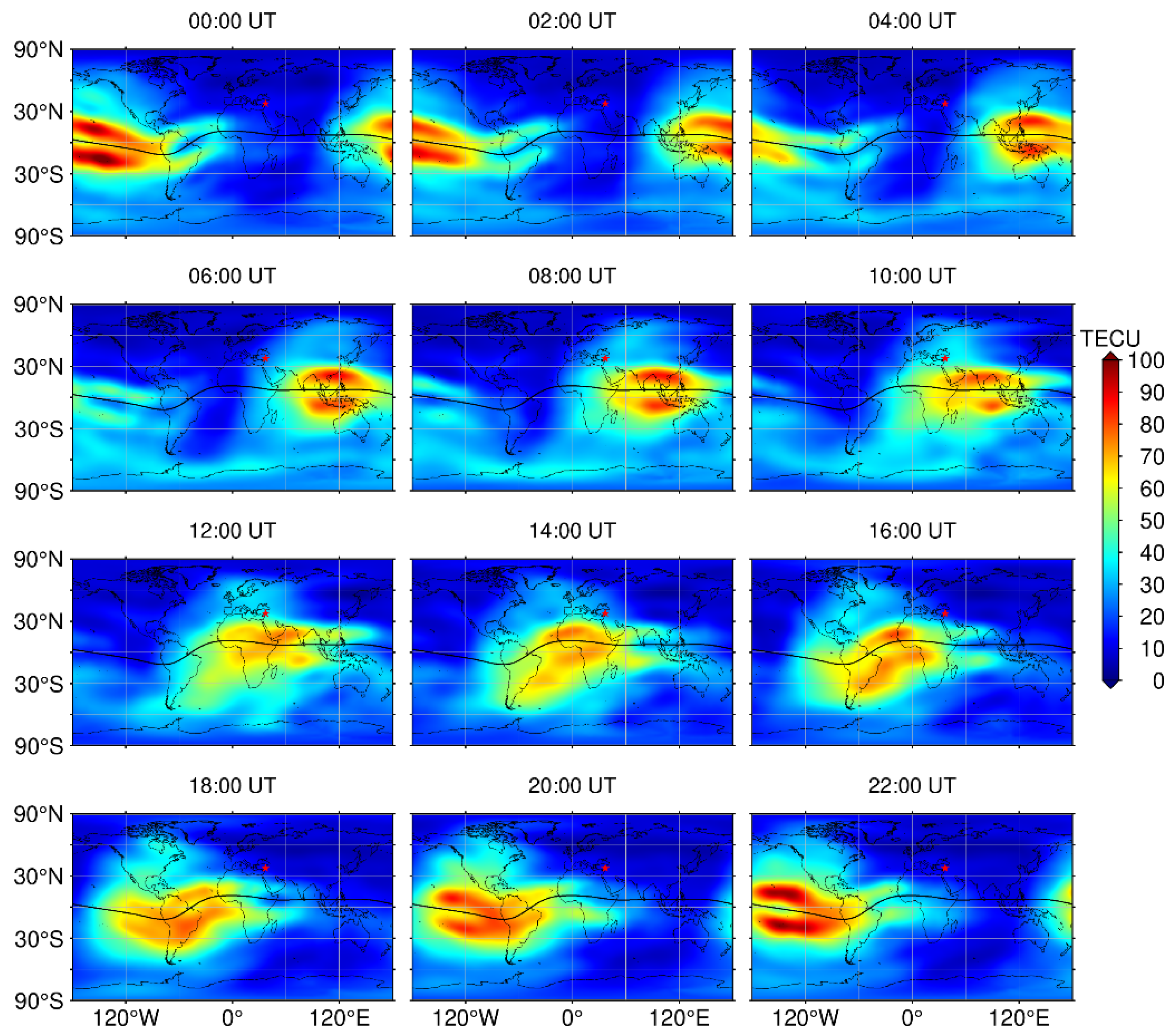
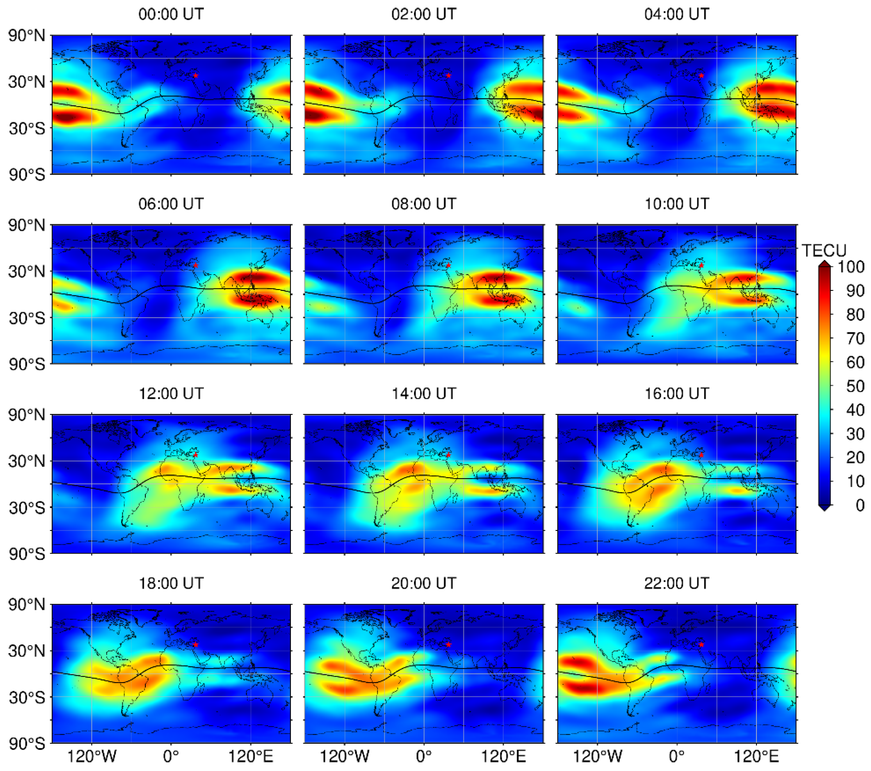
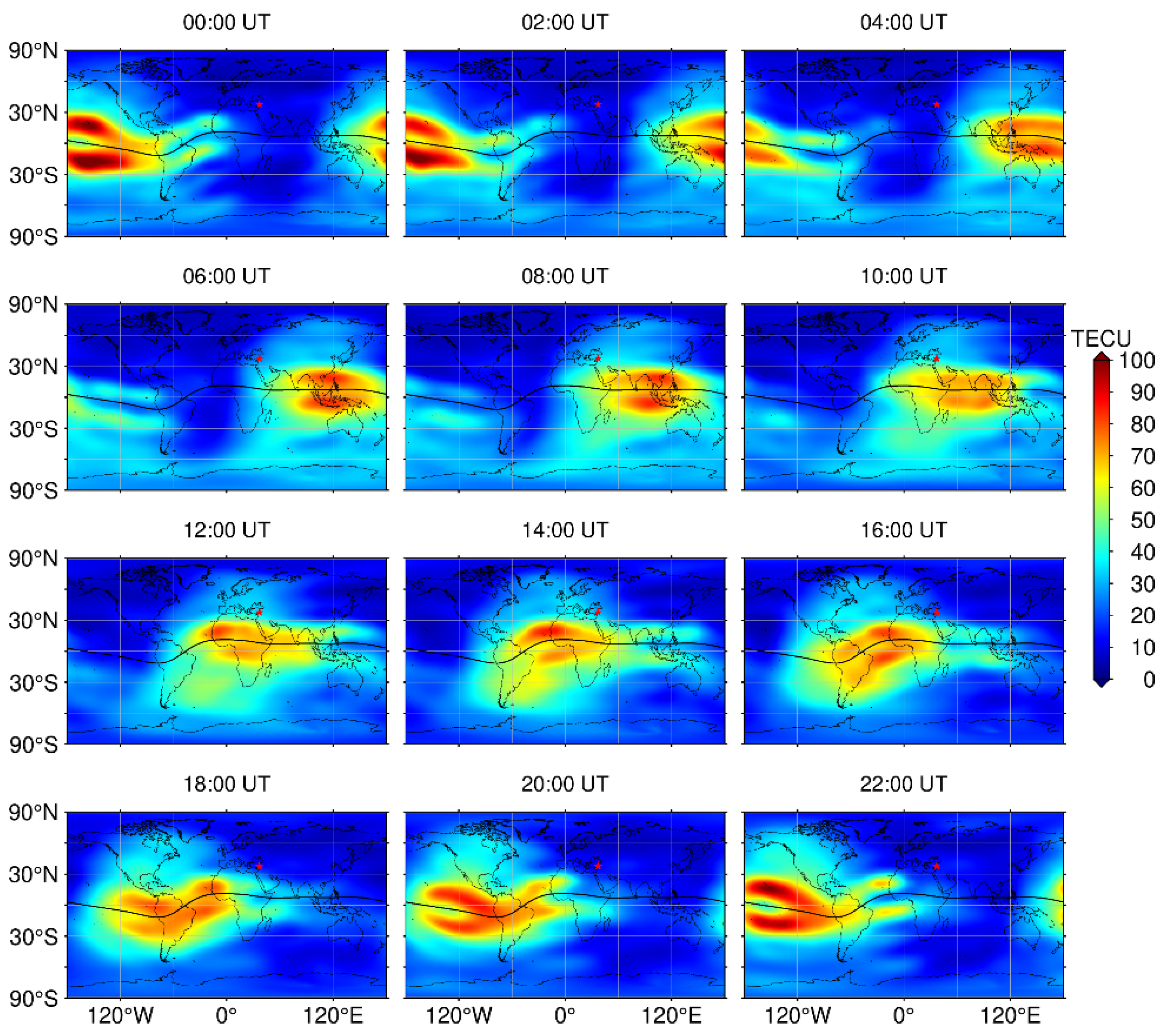
4.3. Global Ionospheric TEC Anomaly Analysis
5. Conclusions
Author Contributions
Funding
Data Availability Statement
Acknowledgments
Conflicts of Interest
References
- Jordan, T.; Chen, Y.-T.; Gasparini, P.; Madariaga, R.; Main, I.; Marzocchi, W.; Papadopoulos, G.; Yamaoka, K.; Zschau, J. Operational Earthquake Forecasting: State of Knowledge and Guidelines for Implementation. Ann. Geophys. 2011. [Google Scholar]
- Shalimov, S.; Gokhberg, M. Lithosphere–ionosphere coupling mechanism and its application to the earthquake in Iran on June 20, 1990. A review of ionospheric measurements and basic assumptions. Phys. Earth Planet. Inter. 1998, 105, 211–218. [Google Scholar] [CrossRef]
- Astafyeva, E.; Heki, K. Vertical TEC over seismically active region during low solar activity. J. Atmos. Sol.-Terr. Phys. 2011, 73, 1643–1652. [Google Scholar] [CrossRef]
- Leonard, R.S.; Barnes, R., Jr. Observation of ionospheric disturbances following the Alaska earthquake. J. Geophys. Res. 1965, 70, 1250–1253. [Google Scholar] [CrossRef]
- Wang, X.; Yang, D.; Zhou, Z.; Cui, J.; Zhou, N.; Shen, X. Features of topside ionospheric background over China and its adjacent areas obtained by the ZH-1 satellite. Chin. J. Geophys. 2021, 64, 391–409. [Google Scholar]
- Liu, J.; Chen, Y.; Pulinets, S.; Tsai, Y.; Chuo, Y. Seismo-ionospheric signatures prior to M ≥ 6.0 Taiwan earthquakes. Geophys. Res. Lett. 2000, 27, 3113–3116. [Google Scholar] [CrossRef]
- Antselevich, M. The influence of Tashkent earthquake on the Earth’s magnetic field and the ionosphere. Tashkent Earthq. 1966, 26, 187–188. [Google Scholar]
- Calais, E.; Minster, J.B. GPS detection of ionospheric perturbations following the January 17, 1994, Northridge earthquake. Geophys. Res. Lett. 1995, 22, 1045–1048. [Google Scholar] [CrossRef]
- Pulinets, S. Seismic activity as a source of the ionospheric variability. Adv. Space Res. 1998, 22, 903–906. [Google Scholar] [CrossRef]
- Zhang, X.; Qian, J.; Ouyang, X.; Cai, J.; Liu, J.; Shen, X.; Zhao, S. Ionospheric electro-magnetic disturbances prior to Yutian 7.2 earthquake in Xinjiang. Ionos. Electro-Magn. 2009, 29, 213–221. [Google Scholar] [CrossRef]
- Zhang, X.-M.; Liu, J.; Shen, X.H.; Parrot, M.; Qian, J.-D.; Ouyang, X.-Y.; Zhao, S.-F.; Huang, J.-P. Ionospheric perturbations associated with the M8. 6 Sumatra earthquake on 28 March 2005. Chin. J. Geophys. 2010, 53, 567–575. [Google Scholar]
- Zhang, Z.-X.; Li, X.-Q.; Wu, S.-G.; Ma, Y.-Q.; Shen, X.-H.; Chen, H.-R.; Wang, P.; You, X.-Z.; Yuan, Y.-H. DEMETER satellite observations of energetic particle prior to Chile earthquake. Chin. J. Geophys. 2012, 55, 1581–1590. [Google Scholar]
- Yan, R.; Wang, L.; Hu, Z.; Liu, D.; Zhang, X.; Zhang, Y. Ionospheric disturbances before and after strong earthquakes based on DEMETER data. Acta Seismol. Sin. 2013, 35, 498–511. [Google Scholar]
- Li, M.; Wang, F.-R.; Zhang, X.-D.; Tan, H.-D.; Kang, C.-L.; Xie, T. Time-spatial statistical characteristics of seismic influence on ionosphere. Prog. Geophys. 2014, 29, 498–504. (In Chinese) [Google Scholar]
- Tong, Y.-J.; Wen, D.-B.; Shu, M. The Discussion on Anomalous Response of Ionospheric VTEC before M7.2 Mexico Earthquake. J. Navig. Position. 2015, 3, 117–121. [Google Scholar]
- Zhang, X.; Liu, J.; Qian, J.; Shen, X.; Cai, J.; Ouyang, X.; Zhao, S. Ionospheric electromagnetic disturbance before Gaize earthquake with MS6. 9, Tibet. Earthquake 2008, 28, 14–22. [Google Scholar]
- Heki, K. Ionospheric electron enhancement preceding the 2011 Tohoku-Oki earthquake. Geophys. Res. Lett. 2011, 38. [Google Scholar] [CrossRef]
- Cahyadi, M.N.; Heki, K. Ionospheric disturbances of the 2007 Bengkulu and the 2005 Nias earthquakes, Sumatra, observed with a regional GPS network. J. Geophys. Res. Space Phys. 2013, 118, 1777–1787. [Google Scholar] [CrossRef]
- Heki, K.; Enomoto, Y. Mw dependence of the preseismic ionospheric electron enhancements. J. Geophys. Res. Space Phys. 2015, 120, 7006–7020. [Google Scholar] [CrossRef]
- Ding, J.; Suo, Y.; Yu, S. Phenomena of geomagnetic and ionospheric anomalies and their relation to earthquakes. Chin. J. Space Sci. 2005, 25, 536–542. [Google Scholar] [CrossRef]
- Zeng, Z.C.; Zhang, B.; Fang, G.Y.; Wang, D.F.; Yin, H.J. An analysis of ionospheric variations before the Wenchuan earthquake with DEMETER data. Chin. J. Geophys. 2009, 52, 13–22. [Google Scholar] [CrossRef]
- Zhang, X.; Liu, J.; Zhao, B.; Xu, T.; Shen, X.; Yao, L. Analysis on ionospheric perturbations before Yushu earthquake. Chin. J. Space Sci. 2014, 34, 822–829. [Google Scholar] [CrossRef]
- Xu, T.; Hu, Y.; Wu, J.; Li, C.; Wu, Z.; Suo, Y.; Feng, J. Statistical analysis of seismo-ionospheric perturbation before 14 Ms ≥ 7.0 strong earthquakes in Chinese subcontinent. Chin. J. Radio. Sci. 2012, 27, 507–512. [Google Scholar]
- Liu, J.; Chen, C.; Tsai, H.; Le, H. A statistical study on seismo-ionospheric anomalies of the total electron content for the period of 56 M ≥ 6.0 earthquakes occurring in China during 1998–2012. Chin. J. Space Sci. 2013, 33, 258–269. [Google Scholar]
- Liu, J.; Wan, W.; Shen, X.; Zhang, X. Spatial-temporal distribution of the ionospheric perturbations prior to Ms ≥ 6.0 earthquakes in China main land. In Proceedings of the EGU General Assembly Conference Abstracts, Vienna, Austria, 12–17 April 2015; p. 1683. [Google Scholar]
- Zou, B.; Guo, J.; Chang, J. Analysis of TEC anomalies before earthquake based on principal component analysis and the sliding inter quartile range method. GNSS World China 2016, 41, 63–69. [Google Scholar]
- Ke, F.; Wang, Y.; Wang, X.; Qian, H.; Shi, C. Statistical analysis of seismo-ionospheric anomalies related to Ms > 5.0 earthquakes in China by GPS TEC. J. Seismol. 2016, 20, 137–149. [Google Scholar] [CrossRef]
- Liu, C.-Y.; Liu, J.-Y.; Chen, Y.-I.; Qin, F.; Chen, W.-S.; Xia, Y.-Q.; Bai, Z.-Q. Statistical analyses on the ionospheric total electron content related to M ≥ 6.0 earthquakes in China during 1998–2015. Terr. Atmos. Ocean. Sci. 2018, 29, 485–498. [Google Scholar] [CrossRef]
- He, L.; Heki, K. Ionospheric anomalies immediately before Mw7.0–8.0 earthquakes. J. Geophys. Res. Space Phys. 2017, 122, 8659–8678. [Google Scholar] [CrossRef]
- Feng, J.; Yuan, Y.; Zhang, T.; Zhang, Z.; Meng, D. Analysis of Ionospheric Anomalies before the Tonga Volcanic Eruption on 15 January 2022. Remote Sens. 2023, 15, 4879. [Google Scholar] [CrossRef]
- Akhoondzadeh, M.; De Santis, A.; Marchetti, D.; Wang, T. Developing a Deep Learning-Based Detector of Magnetic, Ne, Te and TEC Anomalies from Swarm Satellites: The Case of Mw 7.1 2021 Japan Earthquake. Remote Sens. 2022, 14, 1582. [Google Scholar] [CrossRef]
- Yuan, Y. Study on Theories and Methods of Correcting Ionospheric Delay and Monitoring Ionosphere Based on GPS. Ph.D. Thesis, Institute of Geodesy and Geophysics Chinese Academy of Sciences, Wuhan, China, 2002. [Google Scholar]
- Yuan, Y.; Ou, J. Auto-covariance estimation of variable samples (ACEVS) and its application for monitoring random ionospheric disturbances using GPS. J. Geod. 2001, 75, 438–447. [Google Scholar] [CrossRef]
- Akhoondzadeh, M. Kalman Filter, ANN-MLP, LSTM and ACO Methods Showing Anomalous GPS-TEC Variations Concerning Turkey’s Powerful Earthquake (6 February 2023). Remote Sens. 2023, 15, 3061. [Google Scholar] [CrossRef]


| Station | Latitude | Longitude |
|---|---|---|
| bshm | 32.779°N | 35.020°E |
| zeck | 43.788°N | 41.565°E |
| tubi | 40.787°N | 29.451°E |
| mers | 36.566°N | 34.256°E |
| monp | 32.890°N | 116.420°W |
| Date | Sliding Interquartile Range (TECU) | LSTM | BZ (nT) | Kp | DSt (nT) | Ap (nT) | SW (km/s) | F10.7 (sfu) | Solar Activity | Geomagnetic Activity Level |
|---|---|---|---|---|---|---|---|---|---|---|
| 1.18 | +15 | Anomaly | 3.9 | 40 | −10 | 27 | 445 | 213 | Solar flare | Active |
| 1.19 | +5 | Anomaly | 3.8 | 27 | −6 | 12 | 423 | 219 | Solar flare | Active |
| 1.20 | +2.5 | Anomaly | 6 | 27 | 4 | 12 | 444 | 211 | None | Stable |
| 1.21 | +5 | Anomaly | 5.5 | 40 | 4 | 27 | 503 | 202 | None | Active |
| 1.22 | +2.5 | None | 4 | 33 | 1 | 18 | 445 | 192 | Solar flare | Active |
| 1.23 | −1 | None | 9 | 30 | 7 | 15 | 516 | 183 | Solar wind anomaly | Active |
| 1.24 | +2.5 | None | 4.1 | 13 | 3 | 5 | 446 | 175 | None | Stable |
| 1.25 | −1 | Anomaly | 6.7 | 30 | 4 | 15 | 431 | 167 | Solar flare | Active |
| 1.26 | +2.5 | None | 7.1 | 27 | 7 | 12 | 551 | 146 | Solar wind anomaly | Active |
| 1.27 | +2.5 | Anomaly | 6 | 33 | 4 | 18 | 574 | 141 | None | Stable |
| 1.28 | −1 | None | 2.8 | 30 | 7 | 15 | 552 | 133 | None | Active |
| 1.29 | −1 | None | 2.5 | 20 | 8 | 7 | 499 | 133 | None | Stable |
| 1.30 | −1 | Anomaly | 5.4 | 27 | 25 | 12 | 475 | 132 | Solar wind anomaly | Active |
| 1.31 | +2.5 | Anomaly | 3.1 | 33 | 7 | 18 | 484 | 133 | None | Active |
| 2.1 | −1 | None | 0.7 | 27 | 14 | 12 | 430 | 130 | Solar wind anomaly | Active |
| 2.2 | +2.5 | Anomaly | 3.7 | 33 | 0 | 18 | 413 | 131 | None | Active |
| 2.3 | +2.5 | Anomaly | 5.5 | 30 | 18 | 15 | 357 | 131 | None | Active |
| 2.4 | +2.5 | Anomaly | 2.9 | 27 | 2 | 12 | 382 | 135 | None | Stable |
| 2.5 | +2.5 | Anomaly | 6.4 | 20 | 26 | 7 | 358 | 140 | None | Stable |
Disclaimer/Publisher’s Note: The statements, opinions and data contained in all publications are solely those of the individual author(s) and contributor(s) and not of MDPI and/or the editor(s). MDPI and/or the editor(s) disclaim responsibility for any injury to people or property resulting from any ideas, methods, instructions or products referred to in the content. |
© 2023 by the authors. Licensee MDPI, Basel, Switzerland. This article is an open access article distributed under the terms and conditions of the Creative Commons Attribution (CC BY) license (https://creativecommons.org/licenses/by/4.0/).
Share and Cite
Feng, J.; Xiao, Y.; Chen, J.; Sun, S.; Ke, F. A Method for Detecting Ionospheric TEC Anomalies before Earthquake: The Case Study of Ms 7.8 Earthquake, February 06, 2023, Türkiye. Remote Sens. 2023, 15, 5175. https://doi.org/10.3390/rs15215175
Feng J, Xiao Y, Chen J, Sun S, Ke F. A Method for Detecting Ionospheric TEC Anomalies before Earthquake: The Case Study of Ms 7.8 Earthquake, February 06, 2023, Türkiye. Remote Sensing. 2023; 15(21):5175. https://doi.org/10.3390/rs15215175
Chicago/Turabian StyleFeng, Jiandi, Yuan Xiao, Jianghe Chen, Shuyi Sun, and Fuyang Ke. 2023. "A Method for Detecting Ionospheric TEC Anomalies before Earthquake: The Case Study of Ms 7.8 Earthquake, February 06, 2023, Türkiye" Remote Sensing 15, no. 21: 5175. https://doi.org/10.3390/rs15215175
APA StyleFeng, J., Xiao, Y., Chen, J., Sun, S., & Ke, F. (2023). A Method for Detecting Ionospheric TEC Anomalies before Earthquake: The Case Study of Ms 7.8 Earthquake, February 06, 2023, Türkiye. Remote Sensing, 15(21), 5175. https://doi.org/10.3390/rs15215175