Article

A Parallel-Cascaded Ensemble of Machine Learning Models for Crop Type Classification in Google Earth Engine Using Multi-Temporal Sentinel-1/2 and Landsat-8/9 Remote Sensing Data

by
Esmaeil Abdali
1,†,
Mohammad Javad Valadan Zoej
1,
Alireza Taheri Dehkordi
1,† and
Ebrahim Ghaderpour
2,*
1
Department of Photogrammetry and Remote Sensing, K. N. Toosi University of Technology, Tehran 19967-15433, Iran
2
Department of Earth Sciences & CERI Research Center, Sapienza University of Rome, P.le Aldo Moro, 5, 00185 Rome, Italy
*
Author to whom correspondence should be addressed.
These authors contributed equally to this work.
Remote Sens. 2024, 16(1), 127; https://doi.org/10.3390/rs16010127
Submission received: 3 December 2023 / Revised: 25 December 2023 / Accepted: 26 December 2023 / Published: 28 December 2023
(This article belongs to the Section Remote Sensing in Agriculture and Vegetation)

Abstract

:
The accurate mapping of crop types is crucial for ensuring food security. Remote Sensing (RS) satellite data have emerged as a promising tool in this field, offering broad spatial coverage and high temporal frequency. However, there is still a growing need for accurate crop type classification methods using RS data due to the high intra- and inter-class variability of crops. In this vein, the current study proposed a novel Parallel-Cascaded ensemble structure (Pa-PCA-Ca) with seven target classes in Google Earth Engine (GEE). The Pa section consisted of five parallel branches, each generating Probability Maps (PMs) for different target classes using multi-temporal Sentinel-1/2 and Landsat-8/9 satellite images, along with Machine Learning (ML) models. The PMs exhibited high correlation within each target class, necessitating the use of the most relevant information to reduce the input dimensionality in the Ca part. Thereby, Principal Component Analysis (PCA) was employed to extract the top uncorrelated components. These components were then utilized in the Ca structure, and the final classification was performed using another ML model referred to as the Meta-model. The Pa-PCA-Ca model was evaluated using in-situ data collected from extensive field surveys in the northwest part of Iran. The results demonstrated the superior performance of the proposed structure, achieving an Overall Accuracy (OA) of 96.25% and a Kappa coefficient of 0.955. The incorporation of PCA led to an OA improvement of over 6%. Furthermore, the proposed model significantly outperformed conventional classification approaches, which simply stack RS data sources and feed them to a single ML model, resulting in a 10% increase in OA.

Graphical Abstract

1. Introduction

The spatial distribution of crops has undergone significant changes on a global, national, and regional scale due to the combined impacts of climate change and anthropogenic activities [1]. Consequently, accurate and timely mapping of crop types is crucial for ensuring food security, effectively managing of agricultural fields, and achieving sustainable development goals. Additionally, crop type maps provide valuable inputs for environmental models used to study agricultural responses to environmental factors [2]. In contrast to traditional methods such as labor-intensive and time-consuming field surveys, Remote Sensing (RS) satellite data have emerged as a promising tool in crop type mapping by offering large spatial coverage, high temporal frequency, and diverse spatial resolutions [3,4].
RS satellite data can be divided into two main categories: Multispectral (MS) and Synthetic Aperture Radar (SAR) data. Many crop type mapping approaches primarily relied on MS data due to its strong ability to capture the spectral properties of crops and track vegetation phenology. Widely used MS RS data sources include the Moderate Resolution Imaging Spectroradiometer (MODIS) [5,6], Landsat (L) series (particularly L4, 5, 8, and 9) [7,8], and Sentinel-2 (S2) [9,10,11,12,13]. On the other hand, some studies focused solely on SAR data for crop type mapping, with Sentinel-1 (S1) being the most commonly utilized one due to its public availability [14]. This is because SAR data offer the advantage of providing data under various weather and lighting conditions [15]. Furthermore, the backscatter SAR signal is sensitive to surface parameters, such as crop humidity, crop biomass structure, soil conditions, and surface roughness [16,17]. It is worth emphasizing that in the reviewed literature, most papers utilized multi-temporal MS or SAR data to span the entire cropping year. This methodology enables a more comprehensive understanding of phenological changes throughout the growing season, leading to more precise identification of different crop types [9,18].
Synergistic approaches that combine various sources of MS data demonstrated higher overall accuracies than single source approaches in crop classification [19]. This is because MS satellites have different temporal resolutions, which provide enhanced phenological information and, consequently, lead to improved classification accuracy. The most common combination of MS data involves the synergistic use of S2 and L8/9 due to their similar characteristics [20,21]. Additionally, including S1 images in combination with MS data in classification models has the potential to enhance crop mapping accuracies [22]. As mentioned, SAR data capture the physical and structural properties of the crops, complementing the spectral information obtained from MS sensors. In this regard, scholars have commonly employed the combination of S1 with either S2 [23] or L8 [24]. However, there is a limited number of studies that have classified crop types using a multi-source combination of multi-temporal S1/2 and L8/9 data, followed by this article.
The development of multi-temporal multi-source approaches can pose serious challenges due to the substantial volume of RS data that must be stored and processed [25]. However, in recent years, the emergence of Google Earth Engine (GEE), a cloud-based processing platform, has greatly facilitated RS applications [26,27]. GEE has been extensively employed in various fields, including water resources management [28,29], long-term land cover change detection [30], land cover classification [31], insect and disease monitoring [32]. With GEE, users have convenient access to Java and Python Application Programming Interfaces (APIs), eliminating the need to download data for different tasks. As a result, harnessing the capabilities of GEE to develop novel classification approaches with improved accuracy can enable scientists to obtain more reliable results in near real-time earth observation purposes using RS data.
Accurately mapping crop types using RS data is a challenging task due to the high intra- and inter-class variability resulting from crop diversity, environmental conditions, and farming practices [31,33]. To tackle this challenge, most of the articles used pixel-based supervised Machine Learning (ML) classification algorithms which possess the ability to capture nonlinear relationships within the data [34,35]. A significant portion of the literature in this field relies on a single classifier to predict the target class. The commonly utilized models encompass Support Vector Machines (SVM) [36], Random Forests (RF) [37], and Artificial Neural Networks (ANNs) [38]. However, some scholars proposed the structure of an ensemble of ML models, leveraging the complementary information from different classifiers to address the aforementioned challenges, and achieved improved accuracy levels [10,39].
These proposed ensemble structures can be categorized into Parallel (Pa) and Cascaded (Ca) structures [40]. In Pa structures, there are multiple branches, each containing an ML model. To predict the final class of a sample, the predictions from each ML model are combined using simple techniques like majority voting [41]. In the existing literature, Pa structures have primarily been implemented either at the model level or the training data level [42]. At the model level, ML classifiers differ across branches, but input data are the same for each base model within each branch. However, it is important to note that some of the ML models employed in this approach may perform much better than others, resulting in serious uncertainties when they are combined in Pa structure. At the training data level, techniques such as the bagging algorithm (also known as bootstrap aggregation) are employed to train identical ML models using different training data in each branch [43]. While this approach aims to improve performance, the use of a subset of training samples/features prevents the ML models from fully utilizing all of the training data to learn the underlying patterns. Moreover, this strategy required hundreds of models to be trained. Previous scholars did not consider a Pa structure at input data level, in which not only are the entire training data used in each branch, but also the combination of different RS data sources can boost the classification accuracy.
In the reviewed literature, the Pa structure relied on simple techniques like majority voting to predict the class of a sample. However, these simple approaches encounter challenges when dealing with complex classification tasks. To address this, some of the articles proposed a Ca structure, where the outputs of a Pa structure were directly used by another classifier, mainly referred to Meta-model [43,44]. Since the Meta-model itself is an ML model, the process of feature engineering becomes crucial to enhance the final accuracy [45]. In the Ca structure, it is essential for the input features of the Meta-model to exhibit diversity [46]. However, a notable issue arises in which the generated Probability Maps (PM) within each branch exhibit a high correlation among the different classes. Consequently, the direct use of Pa structure’s outputs in the Ca structure can lower the performance of the ensemble model. Previous articles utilized feature extraction algorithms to handle the highly correlated input features of ML models, among which the Principal Component Analysis (PCA) technique exhibited promising performance [47,48]. However, these techniques were used in single-model methodologies and have not yet been employed in an ensemble model structure. Utilizing these techniques effectively mitigates undesired correlations during the learning process of the Meta-model by eliminating redundant and irrelevant features.
In the present work, a novel ensemble framework is proposed, namely a Parallel-PCA-Cascaded (Pa-PCA-Ca) ensemble structure for crop type mapping, with the entire methodology developed and implemented in GEE. In the proposed framework, the outputs of a Pa structure at input data level, after being fed to PCA for redundant information elimination, are used in a Ca structure by a Meta-model. Various ML models, such as RF, SVM, Gradient Boosting Tree (GBT), and Classification And Regression Tree (CART), were employed in the proposed methodology. Additionally, the methodology incorporates different sources of satellite imagery to map different crop types in Mahabad city, Iran. The main contributions of this work are summarized below:
(1)
A novel ensemble ML framework is proposed based on a Pa-Ca structure combined with PCA transformation, which integrates the outputs of MLs and multi-source satellite data for improved crop type classification.
(2)
Both MS and SAR RS satellite imageries (S1/2 and L8/9) were employed, and the proposed method was evaluated using the Ground Truth (GT) data of different crop types collected using extensive field surveys in Mahabad, Iran.
(3)
The study involved conducting a comparative analysis of multiple ML models within the proposed methodology, alongside a comparison between the proposed methodology and two conventional methods used for classifying crop types.

2. Study Area and Datasets
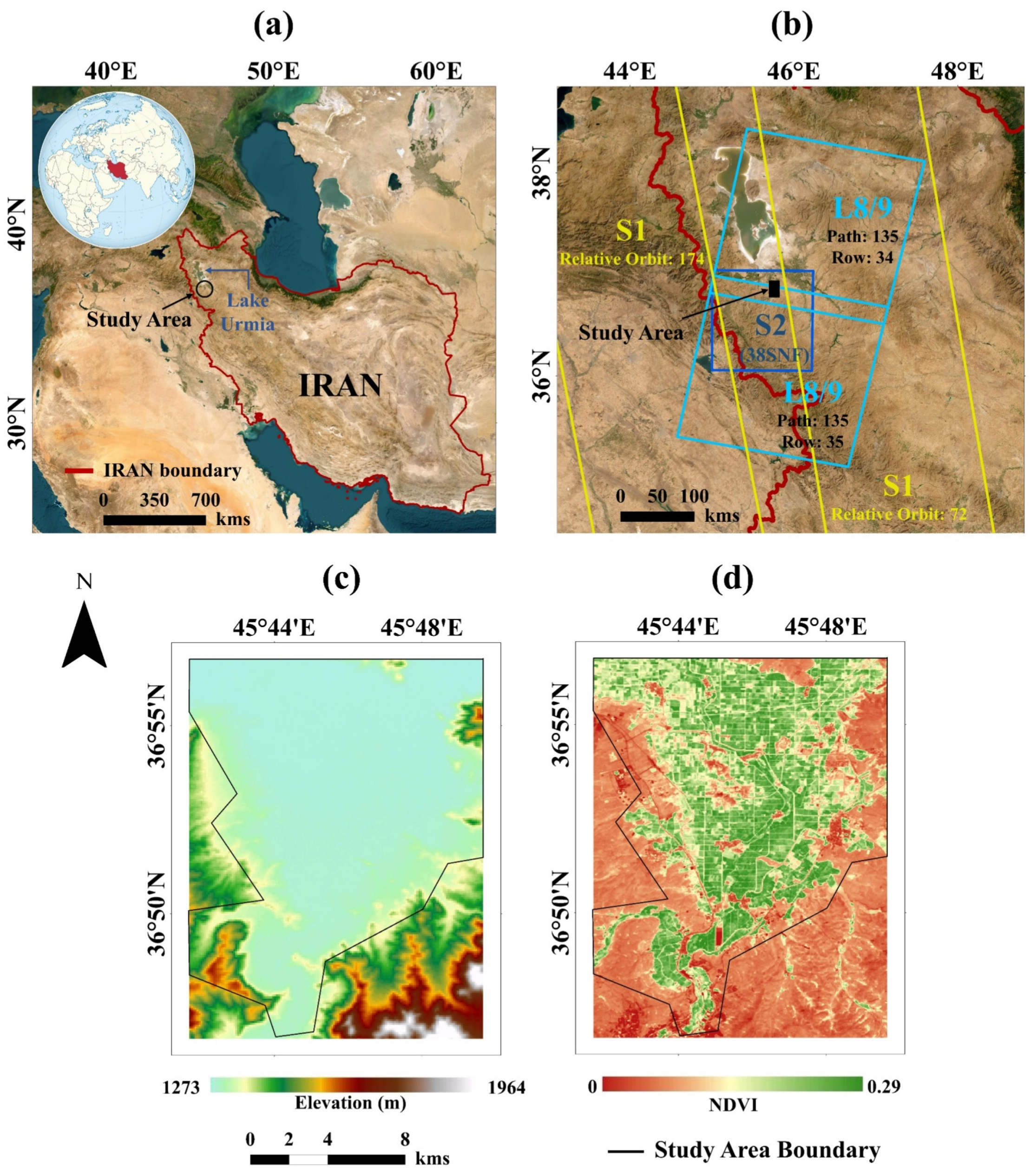
This section introduces the study area and the data sources utilized, which include RS satellite images and GT data.

2.1. Study Area

In this paper, the upstream agricultural lands of Mahabad city were selected for evaluating the proposed methodology. The study region is in the northwest part of Iran and lies south of Lake Urmia in a fertile plain (Figure 1a,b), approximately 1400 m above sea level (Figure 1c). The average annual temperature and rainfall of this region are 12 °C and 390 mm, respectively [49]. Considering the population living in the surrounding areas of the study site, about 200,000 people are influenced by the agricultural products of this region. Additionally, this region’s croplands directly impact the water dynamics of Lake Urmia, contributing to its gradual desiccation [50]. Figure 1d illustrates the 10-year average (2013–2023) of Normalized Difference Vegetation Index (NDVI) derived from L8/9 data. The surrounding regions of the area are mainly covered by rocks and mountains. Therefore, the inside region of the boundary depicted in Figure 1c,d was chosen as the study site. The majority of agricultural lands are situated in the central parts, whereas the surrounding regions are mainly related to bare lands and urban areas. So, there is a diverse ecosystem within the area, encompassing agricultural lands with various crop types, bare soil, and urban areas. Various agricultural products are cultivated in this region, including both autumn and spring crops. Wheat is the main autumn crop, while beet, alfalfa, corn, and onion are the main spring crops. Additionally, there are extensive garden lands of apple in this region. Following the agricultural calendar, the cultivation of autumn crops begins in November, while the harvesting of spring crops continues until the end of December. Consequently, the cropping year in this region spans from November of the previous year to December of the following year.

2.2. Datasets

Three sources of RS satellite data were utilized (S1, S2, and L8/9). Moreover, the proposed Pa-PCA-Ca ensemble structure is a supervised classification technique, meaning that it needed Ground Truth (GT) data for model calibration and validation.

2.2.1. Satellite RS Data

Satellite imageries of two MS Landsat (L) missions were one of the optical satellite data sources utilized in this study. When conducting this research, only L8 and L9 satellites were active, launched on February 11, 2013, and September 27, 2021, respectively [51]. This study utilized the Surface Reflectance (SR) products of L8/9, which are available after the Land SR Code (LaSRC) correction incorporating radiometric, terrain, and atmospheric corrections [52]. L8 and L9 missions have a spatial resolution of 30 m. Besides, both include six spectral bands, encompassing the visible, Near Infrared (NIR), and Shortwave Infrared (SWIR) regions, with a spectral range extending from 482 to 2200 nm (Table 1). It is important to mention that the coastal aerosol band of L8/9 was not utilized. Each of these missions provides a temporal resolution of 16 days, which is reduced to 8 days when combined. So, because of their similar spatial, spectral, and temporal characteristics, their combination was considered as a single dataset, hereafter referred to as L8/9. Figure 1b illustrates that the study site is covered by two L8/9 scenes (with a path number of 135 and row numbers 34 and 35).
In this paper, S2 MS images were used as another source of optical satellite data, which are acquired through a Multi-Spectral Instrument (MSI) sensor. The S2 mission consists of two identical satellites, S2-A and S2-B, launched on 23 June 2015, and 7 March 2017. Each satellite has a 10-day repeat cycle, which is reduced to 5 days when both are used. The MSI has 13 spectral bands, with three dedicated to atmospheric applications (with a spatial resolution of 60 m). The other ten bands cover the visible, Near Infrared (NIR), and Shortwave Infrared (SWIR) regions, spanning from 496 to 2200 nm, with spatial resolutions of 10 and 20 m [53]. This study utilized S2 level-2A data which provide SR values after radiometric, terrain, and atmospheric corrections using the Sen2Core algorithm [54]. As can be seen in Figure 1b, the study site is entirely covered by a single S2 image with a granule number of 38SNF.
This study also utilized the S1 satellite as an SAR data source. S1 is the first mission of the Copernicus program developed by the European Space Agency (ESA). This mission includes a constellation of two identical satellites: S1-A (launched on 3 April 2014) and S1-B (launched on 26 April 2016). The dual-satellite constellation provides a 6-day repeat cycle. The S1 satellites are equipped with a C-band (5.405 GHz) SAR instrument, which can collect data in any weather conditions and at any time of the day or night [55]. The S1 Ground Range Detected (GRD) product is used for this study, which provides two polarizations: Vertical-Vertical (VV) and Vertical-Horizontal (VH) in Interferometric Wide (IW) swath mode. This product is available through GEE after being preprocessed using the S1 Toolbox (S1TBX), providing a spatial resolution of 10 m [56]. The preprocessing includes thermal noise removal, radiometric calibration, and terrain correction. Since the majority of the available S1 images over the study site were acquired in an ascending orbit, this study only utilized S1 data acquired in an ascending orbit. The study site was entirely covered by two ascending orbits with relative orbit numbers of 72 and 174 (Figure 1b), resulting in multiple S1 scenes capturing the study site.

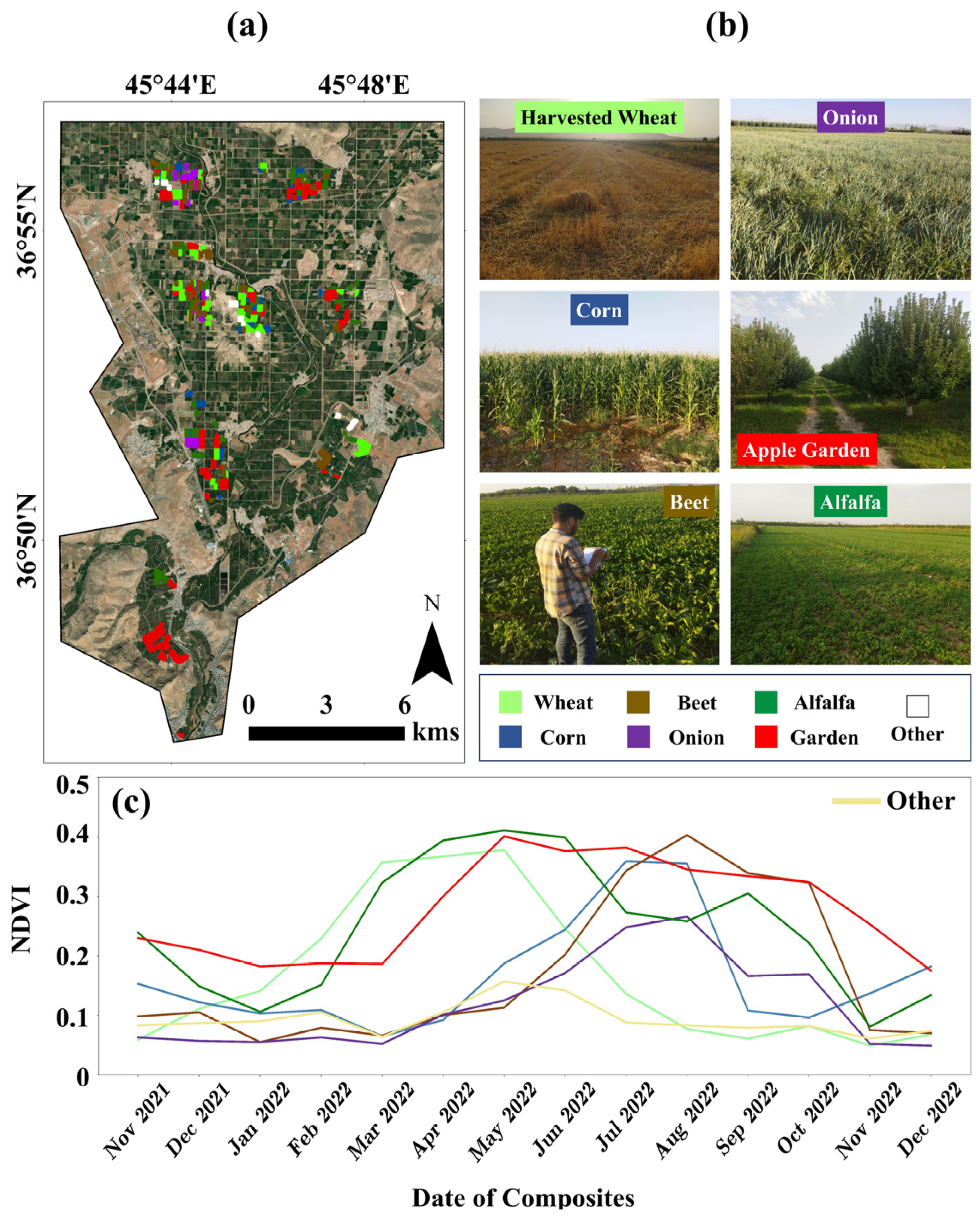
2.2.2. Reference GT Data

The proposed method relies on supervised classification, which requires training data of high reliability. Multiple field surveys were conducted in the study area between June 2022 and September 2022 to collect reliable GT data for model validation and calibration. This period coincides with the peak growth period of autumn and spring products in the study site. The distribution of GT samples and some images during field surveys can be seen in Figure 2. Field visits were done so that the ground data have appropriate distribution in the study site. During the field surveys, 315 polygons were recorded, which were related to various classes such as ‘Wheat’, ‘Corn’, ‘Beet’, ‘Onion’, ‘Alfalfa’, ‘Garden’, and ‘Other’. The ‘Other’ class encompasses bare soil, urban areas, and water bodies, while the ‘Garden’ class comprises apple gardens mostly. For each polygon, the corner coordinates of each field were recorded using a handheld GPS device (Garmin eTrex 20x) with a spatial accuracy of less than 5 m. To prevent the mixed pixels effect, the corner pixels were recorded with at least a 30 m distance from the surrounding landcover classes. Table 2 indicates the number of sample points (in a 30-m resolution) in each class derived from field surveys. Figure 2c also illustrates the NDVI behavior of randomly selected samples from each target class derived from the monthly medians of L8/9 (as mentioned in Section 3.1). The reference dataset was divided into two sections, 70% as training and 30% as validation. Training data were used for model calibration, while validation data were used in the accuracy assessment with no inference in the training phase.

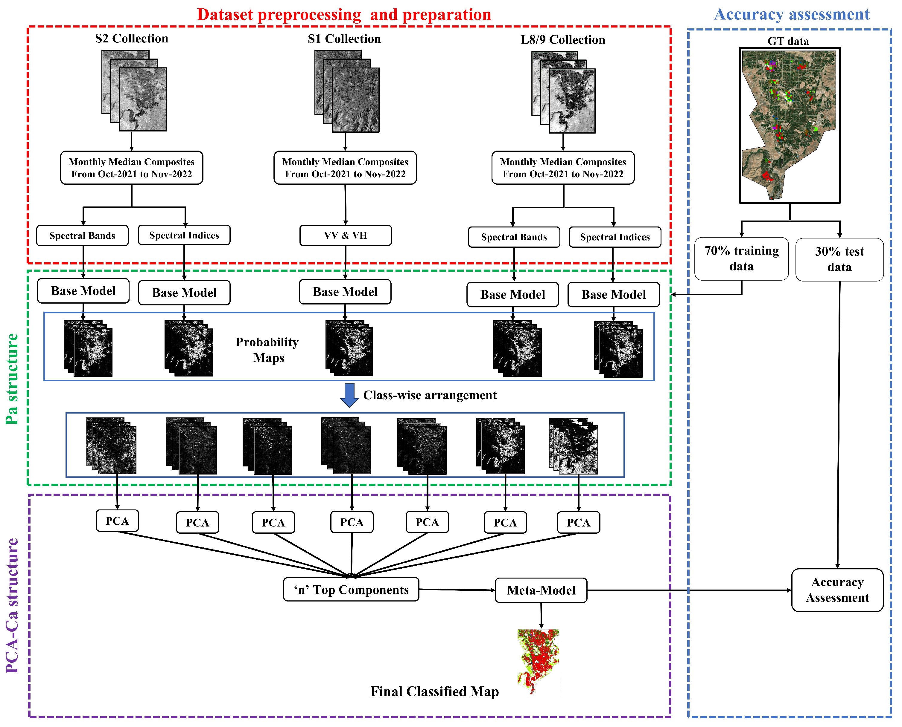
3. Proposed Framework

As mentioned in the introduction, this study aimed to propose a novel Pa-PCA-Ca ensemble structure for crop type classification in RS satellite data. The outline of the proposed methodology can be seen in Figure 3, which consists of four main steps: (1) dataset preprocessing and preparation, (2) Pa structure, (3) PCA-Ca structure, and (4) accuracy assessment. Each of the steps is going to be elaborated more fully in the following sections. It should be emphasized that the entire procedure was designed based on the capabilities of GEE and fully implemented within this cloud-based platform.

3.1. Dataset Preprocessing and Preparation

As mentioned earlier, three sources of satellite data were utilized in this study: S1, S2, and L8/9. S2 and L8/9 images belong to the optical type of satellite data, which face limitations due to cloud coverage, which hinders the full observation of the study site. Consequently, any images with a cloud coverage of more than 10% were excluded. Additionally, clouds and cloud shadows were eliminated from each scene by utilizing the pixel quality attributes which are available alongside each S2 or L8/9 image (‘QA60’ band for S2 and ‘QA_PIXEL’ for L8/9). However, the removal of cloudy pixels resulted in data gaps within some images across the study site. Furthermore, it is important to mention that the study area was covered with multiple image scenes in some satellite missions like S1 and L8/9, as depicted in Figure 1b. Consequently, this study used a monthly median compositing approach to generate the input satellite images for the ML models. This approach has been proved to be effective in similar studies [57]. The monthly composites ensure the gap-free images of the study site and also aid in reducing the possible sensor-related noises in optical datasets (S2 and L8/9) and speckle noise in S1 SAR data.
Note that multi-temporal satellite imageries were mainly utilized in the literature for crop type classification. This is because multi-temporal data take into account crop growth patterns and phenological information [37]. Therefore, images from ‘1 November 2021’ to ’30 December 2022’ were selected (based on the aforementioned conditions). This period covers the entire 2022 cropping year of the study site, which is the year of GT data collection. As a result, 14 monthly median composites were generated for each data collection (S1, S2, and L8/9). Considering the varying spatial resolutions among the satellite data sources, all the median composites were resampled using bilinear technique to a spatial resolution of 30 m, based on the lowest spatial resolution provided by L8/9 [58].
As mentioned in the introduction, the paper proposes a Pa structure at the data level. This means that each prepared multi-temporal composite of S1, S2, and L8/9 data was separately inputted into the ML models. However, for the optical datasets (S2 and L8/9), in addition to the spectral bands, Spectral Indices (SIs) were also utilized to enhance the classification accuracy. This is because previous studies have demonstrated that SIs can improve the identification of complex crop type classes [59,60], as they are designed to highlight specific objects of interest in optical data [61]. In this vein, five of the most commonly used SIs in the literature were employed: Normalized Difference Vegetation Index (NDVI) [62], Normalized Difference Water Index (NDWI) [63], Normalized Difference Built-up Index (NDBI) [64], Soil Adjusted Vegetation Index (SAVI) [65], and Enhanced Vegetation Index (EVI) [66]. All of these SIs were extracted from both the monthly composites of S2 and L8/9 data. The mathematical formulas for each index are provided in Table A1. It should be noted that no additional features were extracted from the S1 bands (VV and VH). This is because numerous studies have demonstrated that these specific bands contain sufficient information for land cover mapping, making additional feature extraction from them unnecessary [67]. In summary, five Feature Collections (FCs) were generated as inputs to the ML models, which are presented in Table 3.

3.2. Pa Structure

This study introduced a Pa structure at the data level. This means that, unlike previous studies, each prepared FC in Table 3 was fed to an ML model. This approach allows for the utilization of the strengths of different datasets simultaneously. Additionally, since there is a specific FC in each branch, the Pa structure can achieve higher accuracies compared to the conventional image stacking approach, which introduces unnecessary redundancy and reduces computational efficiency during the classification process. There is a total of five different FCs, resulting in five branches within the Pa structure.
In this study, four widely used ML models in crop classification, including CART, SVM, RF, and GBT, were assessed to find the optimal models in each branch of Pa structure. The CART algorithm is a statistical method which identifies target classes by finding the common characteristics of each class [68]. This method has been widely used in land cover classification due to its simple design and computational efficiency [69]. The tree Maximum Nodes (MN) and Minimum Leaf Population (MLP) are two of the main parameters of this method that must be set.
SVM is another ML method that determines the best possible hyperplane to classify different samples into specific classes based on the input features [70]. This approach offers remarkable advantages in dealing with complex problems, limited sample sizes, and high-dimensional data. When using SVM, the main parameters that need to be modified are the Gamma (G) value and the Cost (C) parameter. Based on the proven performance in the previous articles, the kernel function was set to ‘Radial Basis Function’ (RBF) [71].
RF is an ensemble method that creates multiple decision trees to make predictions. RF has a bagging approach, meaning each tree is built using a random subset of training samples. During prediction, each tree in the forest independently makes a prediction, and the final output is determined by majority voting. The Number of Trees (NT), the Maximum Nodes (MN), and the Variables Per Split (VPS) are the parameters that must be set in this method [72].
GBT is an ensemble algorithm that combines gradient boosting with decision trees. It builds trees sequentially to correct errors made by previous trees. GBT captures complex relationships, processes data sets, and handles missing values automatically [73]. The parameters needing to be set in this classifier are the Number of Trees (NT), the Shrinkage (SH), and the Maximum Nodes (MN).
To select the best model in each branch of the Pa structure, each of the aforementioned ML models is separately evaluated in each branch. The model that achieves the highest accuracy is chosen as the base model for that particular branch. This approach is adopted because some ML models exhibit poorer performance compared to others. Consequently, their simultaneous use alongside other ML models can negatively impact the results. To this end, the hyperparameters of each ML model in each branch were first determined using a five-fold cross-validation approach with the aid of a grid search technique. This involves randomly dividing the training data into five folds. During each iteration, one-fold is held out for validation, while the remaining k-1 folds are used to train the algorithms in each branch using the hyperparameters from the search space. This process is repeated k times, and the best hyperparameters are selected based on the average classification accuracy. The model that achieves the highest classification accuracy on the five-fold cross-validation, along with its optimal hyperparameters, is selected as the base model in each branch. It is important to mention that the same randomly selected five-folds of training data were utilized in all five branches of the Pa structure. Table 4 provides an overview of the hyperparameters of the ML models and their corresponding search space.
After selecting the best model in each branch, each ML model is trained with the same training dataset, which accounts for 70% of the reference dataset. The outcome of each branch in the classification process is a Probability Map (PM) for each class. These PMs contain bands equal to the number of classes (seven in this study). The pixel values in the PMs represent the probability of each pixel belonging to different classes. Since there are five branches in the proposed Pa structure, there are five sets of PMs, each consisting of seven bands. In the next step, these PMs are utilized in the PCA-Ca structure for the final classification.

3.3. PCA-Ca

The generated PMs from different branches within the Pa structure exhibit a strong correlation for each class. For example, the PMs corresponding to the ‘Wheat’ class across different branches show similarities. This can also be concluded from the previous articles in the literature, which suggests that different RS data sources often produce similar outcomes [74]. To address this issue, the current study incorporates Principal Component Analysis (PCA) on the PMs of the Pa structure for each class. PCA is a linear orthogonal transformation technique commonly used for high-dimensional datasets [75]. It involves transforming the input feature space into a new space where the features are uncorrelated. In this study, the bands corresponding to the same class from the five branches are stacked (referred to as class-wise arrangement in Figure 3), resulting in seven new PMs (number of target classes), each consisting of five bands (number of branches). PCA is then applied to the PMs of each class, generating seven new collections, each comprising five uncorrelated bands known as principal components. The top ‘n’ components from each new collection are stacked together to form a probability cube, which is utilized as an input to the Meta-model, referred to as the Ca structure, for classifying different crop types. The value of ‘n’ is determined through a grid search ranging from 1 to 5 (number of branches) using five-fold cross validation of training data.
For the selection of the best Meta-model, the same methodology was applied as in the Pa structure. Specifically, the PMs from the five Pa branches were fed to the four mentioned ML models (CART, SVM, RF, and GBT). It is worth noting that PCA was not employed on the PMs at this stage for a better evaluation of its effect on the Meta-model performance. Using the identical methodology as described in the Pa structure, the hyperparameters of each model were determined using a five-fold cross-validation technique and a grid search approach with the grid search space outlined in Table 4. The model that achieved the highest average classification accuracy was selected as the Meta-model. Once the best model was chosen, the Meta-model was trained using the entire training dataset, which accounted for 70% of the reference dataset. It is important to emphasize that the Meta-model was also trained using the same training data as the branches.
This study evaluated various model architectures to demonstrate the superior performance of the proposed methodology. These different model architectures are outlined in Table 5. Model No. 3 represents a conventional approach of crop type classification, where all input FCs (FC1–FC5) were simply stacked and a single ML model was used for classification. Additionally, to investigate the impact of PCA in traditional approaches, another model architecture was tested (Model No. 4). In this architecture, the top components resulting from the PCA transformation of the input FCs (FC1–FC5) were fed to a single ML model for the final classification.

3.4. Accuracy Assessment

To assess the performance of the proposed framework, the Confusion Matrix (CM) of the classification and various CM-derived parameters were utilized. These parameters included Overall Accuracy (OA), Kappa coefficient, Producer’s Accuracy (PA), and User’s Accuracy (UA). Figure A1 (in Appendix A) illustrates a hypothetical CM for n classes. Equations (A1)–(A4) (in Appendix A) also present the formulas for calculating the aforementioned metrics directly from the CM. It is important to highlight that the accuracy assessment was performed using a validation dataset (30% of the reference dataset). The validation dataset was not used during the training phase or model development. It should be highlighted that the Pearson Correlation Coefficient (PCC) was also utilized to investigate the correlation between the PMs of the Pa structure within each class. This analysis was conducted to justify the need for employing the PCA technique in the proposed methodology.

4. Results

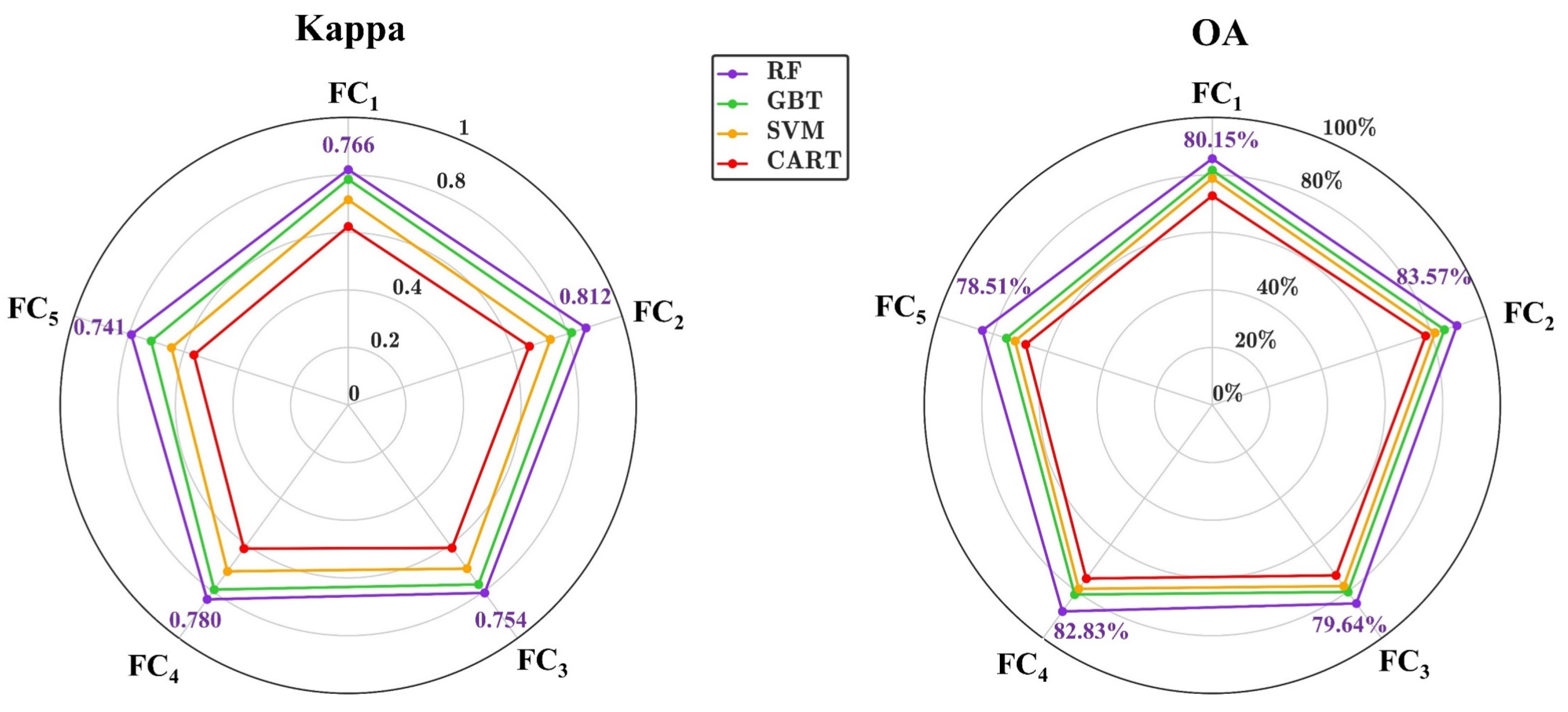
4.1. Base Model Selection in Pa Structure

As mentioned in Section 3.2, the best base model in each branch of Pa structure was determined through 5-fold cross-validation using the training data. The proposed Pa structure consisted of 5 branches, each utilizing different FCs (FC1–5) for model development. Figure 4 illustrates the averaged values of OA and Kappa for various ML models. The optimal hyperparameters of each model were found using the described approach in Section 3.2. It can be observed that the RF model outperformed other ML models in all branches. For instance, RF achieved OA values of 80.15%, 83.57%, 79.64%, 82.83%, and 78.51% in FC1–5 branches, respectively. Similarly, the Kappa values were 0.766, 0.812, 0.754, 0.780, and 0.741, respectively. Therefore, RF was selected as the base model for all Pa branches. Following RF, the GBT, SVM, and CART models ranked next. Moreover, among the branches, FC2 demonstrated the highest accuracy in terms of both OA and Kappa for each ML model. FC4, FC1, FC3, and FC5 were ranked next. The results also indicated that the optical FCs (FC1–4) performed better compared to the SAR FC (FC5). Similarly, the S2 FCs (FC1,2) exhibited better performance than the L8/9 FCs (FC3,4). Furthermore, the index-based FCs (FC2 and FC4) demonstrated superior performance compared to the spectral-based FCs (FC1 and FC3) in optical RS data. It should be noted that the optimal hyperparameters of RF in each branch were as follows: FC1 [NT: 200, MN: 1, VPS:], FC2 [NT: 100, MN: 2, VPS: 1], FC3 [NT:300, MN: 1, VPS: 1], FC4 [NT:200, MN: 1, VPS: 1], and FC5 [NT:200, MN: 2, VPS: 2].

4.2. Meta Model Selection in Ca Structure

After selecting the base model for each branch, the Meta-model in the Ca structure was determined using the same approach mentioned in Section 3.3. It is important to note that in this stage, PCA was not applied to the output PMs of each branch. In other words, PMs of all branches were directly fed to the ML model. This was done to better show the improvements caused by PCA technique in the next sections. Figure 5 illustrates the performance of different ML models in the Ca structure in terms of OA and Kappa. The optimal hyperparameters of each model were found using the described approach in Section 3.3. The RF algorithm outperformed other ML techniques as the Meta-model in the Ca structure. It achieved an OA of 92.56% and a Kappa of 0.911. The GBT and SVM classifiers ranked second and third, with OA values of 90.13% and 85.76%, respectively, and Kappa values of 0.893 and 0.819, respectively. The classifier with the lowest performance was the CART algorithm, which attained an OA of 77.32% and a Kappa of 0.726. Therefore, RF was selected as the Meta-model in the proposed ensemble structure of this article. It should be noted that the optimal hyperparameters of RF as the Meta-model were [NT: 300, MN: 1, VPS: 1].

4.3. Input Data Level Ensemble in Pa-Ca Structure

As mentioned in Section 3.1, the proposed methodology used five FCs (FC1–FC5) in the Pa structure. Figure 6 compares the performance of the Pa-Ca structure (without using PCA technique) for different FCs based on the validation dataset. It should be highlighted that based on the results of Section 4.1 and Section 4.2, RF was selected as the base model and Meta-model in the Pa-Ca structure. Moreover, when there is only a single FC, there would be no Ca structure, and RF is directly implemented to obtain the results. For example, when FC5 is used, only a single RF with optimized hyperparameters is used.
As can be seen (Figure 6), when only a single FC is used, the lowest classification accuracies were obtained. Among the cases of using a single FC, FC2 achieved the highest OA (81.87%) and Kappa (0.782). In contrast, the S1-related FC (FC5) achieved the lowest performance with an OA of 76.68% and a Kappa of 0.721. The results also indicate that among the single FCs, FCs of SIs (FC2, FC4) generally yield better accuracies than FCs of raw spectral bands (FC1, FC3). Additionally, S2-related FCs generally performed better than L8/9 FCs. The same results were also achieved in Figure 4.
All the single FC cases only used the RF model for classification. It can be seen in Figure 6 that when more FCs are used in a Pa-Ca structure, the OA and Kappa values showed significant improvements. This proves the performance of the proposed Pa-Ca structure, which benefits from using different satellite data sources in each branch for crop type classification. By keeping FC5 fixed and combining it with other FCs, the combination of FC2+FC5 in the Pa-Ca structure achieved the highest accuracy, with an OA of 87.58% and a Kappa of 0.851. The results also indicate that using the Pa-Ca approach with all five designed branches achieved the highest OA (91.13%) and Kappa (0.893). As a result, the best case (FC1+ FC2+ FC3+ FC4+ FC5) is selected as the input features of the proposed Pa-Ca ensemble structure in the rest of the paper. In the next step, the effect of employing the PCA technique on the outputs of the Pa section of the proposed methodology is further discussed.

4.4. Pa-PCA-Ca Structure

As mentioned in Section 3.3, the current study employed the PCA technique on the output PMs of different classes. This was done due to the high PCC observed between the output PMs of different branches within each class (Figure 7). For instance, in the ‘Wheat’ class, the PM map of the FC2 branch demonstrated a PCC of 0.89 with the PM of the FC1 branch. The PCC values were 0.85, 0.91, and 0.65 when comparing the PM of FC2 with FC3, FC4, and FC5, respectively. Notably, the optical FCs exhibited stronger correlation among themselves compared to the SAR-based FC (FC5). The PCCs between the output PMs of optical FCs (FC1–4) ranged from 0.71 (FC3 against FC2 and FC4 in the corn class) to 0.96 (FC3 against FC4 in the garden class). However, the PCCs between SAR-based FCs (FC5) and optical FCs (FC1–4) ranged from 0.58 (FC5 against FC1 and FC2 in the ‘Corn’ and ‘Alfalfa’ classes, respectively) to 0.85 (FC5 against FC3 in the ‘Garden’ class). Based on these PCCs, it can be concluded that the PMs of different branches exhibited a high correlation, leading to redundancy in the input FCs of the RF model in the Ca structure. Therefore, employing PCA on the outputs of the Pa structure was necessary to enhance the performance of the Meta-model.
To employ PCA on the output PMs of the Pa structure and feed them into the Ca structure, the top ‘n’ components were selected for each class. To determine the optimal value for ‘n’, as described in Section 3.3, a grid search was conducted using 5-fold cross-validation on the training data. Table 6 presents the effect of ‘n’ on OA and Kappa. As shown, when ‘n’ was set to 1 (using only the first output component of PCA for each class), the classification accuracy experienced a 4.88% increase in OA (from 92.56% to 97.44%) and 0.050 increase in Kappa (from 0.911 to 0.961) compared to the Pa-Ca structure. This indicated that PCA led to a significant improvement in Meta-model performance. Increasing the value of ‘n’ to values of more than 1 did not guarantee higher accuracies compared to the Pa-Ca case. Therefore, ‘n’ was set to 1 in the proposed methodology, and the remaining results in this article are based on this value.
Figure 8 compares the UA and PA of different target classes for the proposed methodology (Pa-PCA-Ca (n = 1)) with the Pa-Ca structure. As can be seen, considering the UA metric, in the Pa-Ca model, the ‘Beet’ class achieved the highest UA of 94.15%, while the ‘Onion’ class achieved the lowest UA of 86.31%. However, employing the PCA technique led to a significant increase in accuracy for all classes, where the ‘Wheat’ class achieved the highest UA of 97.54%, while the ‘Other’ class achieved the lowest UA of 91.97%. The highest increase was observed in the ‘Onion’ class, with an improvement of 9.29% from 86.31% to 95.60%.
The same conclusions can also be drawn for the PA metric (Figure 8). Employing PCA resulted in a significant improvement in accuracy for all classes, with the ‘Onion’ class showing the highest improvement of 6.55% from 90.11% to 96.66%. The results indicate that the PCA technique effectively improves the performance of the Meta-model in the Ca structure, which can also be supported by the OA and Kappa values obtained using 5-fold cross-validation of the training data in Table 6.
The final output PMs of the proposed Pa-PCA-Ca model were also compared with the output PMs of the Pa-Ca model to investigate the effect of the PCA technique. Figure 9 illustrates the “First Max” (refers to the highest probability of each pixel belonging to a specific target class), and the “Second Max” (refers to the second-highest probability of each pixel belonging to another target class), along with their difference. A model is considered to better discriminate the target classes when the highest probability of each pixel is significantly larger than the second-highest value. In other words, the model can assign higher certainty to each pixel when the highest probability is substantially greater than the second highest probability.
As shown in Figure 9, when PCA is applied in the proposed methodology, the "First Max" values increased in most of the study area, while the “Second Max” probabilities decreased substantially in the region. This is further supported by the comparison of the histogram plots of the “difference” maps. The absolute skewness value of 1.75 indicated that the majority of the data points were concentrated towards the right side in the Pa-PCA-Ca model, compared to the Pa-Ca model with an absolute skewness value of 0.19. This suggests that the “difference” map between these two cases indicated larger values for the Pa-PCA-Ca model, indicating that the PCA technique led to a decrease in classification uncertainty, which resulted in higher classification accuracies.
The final crop type maps of the study site are presented in Figure 10, showcasing the outcomes of the proposed method (Pa-PCA-Ca). The quantitative analysis revealed that the proposed method outperformed the Pa-Ca structure in terms of accuracy, thanks to the integration of PCA. The visual representations in Figure 10 also confirm the numerical findings, demonstrating the effectiveness of the proposed methodology (Pa-PCA-Ca) in generating more precise classification maps compared to the Pa-Ca structure. By employing PCA, the presence of noisy points in the pixel-based classification results was notably reduced, which can be attributed to the reduction in uncertainty, as depicted in Figure 9.

4.5. Comparison to Conventional Approaches

As mentioned in Section 3.3 (Table 5), two additional conventional model architectures were utilized to prove the superior performance of the proposed methodology. In these models, RF was chosen as the ML model for classification. Figure 11 displays the CMs of the four model architectures. It is evident that the proposed method achieved an OA that was approximately 10% and 9% higher compared to the conventional feature stacking approach without and with PCA, respectively. The results demonstrated that the proposed methodology displayed improved discrimination across all targets by correctly classifying a higher number of validation samples in each class (identified by the main diagonal elements) compared to the other methods. This indicates that the proposed method effectively accounted for both intra-class and inter-class variabilities of different crop types, resulting in its superior performance.

5. Discussion

5.1. Base Models and Meta-Model

This study introduces a novel ensemble structure for classifying crop types using multi-source and multi-temporal S1, S2, and L8/9 satellite data. The proposed structure consists of two parts: Pa and PCA-Ca. The Pa structure generates inputs for the second part, and accurate outputs from Pa enhance the inputs for PCA-Ca, leading to an improved classification performance. To ensure optimal outputs from the Pa structure, the best performing ML model was utilized in each branch for each specific FC (FC1–5 in Table 3). The selection of the best performing ML model in each branch of the Pa structure mitigates any negative impact from low-performing models when they are combined in the PCA-Ca part. The findings in Figure 4 demonstrated that the RF model outperformed GBT, SVM, and CART in all branches, indicating its superior accuracy in classifying crop types across various optical and SAR-based FCs (FC1–5 in Table 3). Previous studies have also recognized RF as the top-performing ML model for crop type classification [20,40,44,48].
Furthermore, the Meta-model within the Ca structure directly generates the final classification outcomes. Similar to the Pa part, the best performing model within the Ca structure was chosen from RF, GBT, SVM, and CART. The RF model also demonstrated superior performance among these ML models within the Ca structure as well, as indicated in Figure 5. As a result, RF was chosen as the base model in the Pa structure and as the Meta-model in the Ca structure. The same conclusion was mentioned by other articles in this field for selecting the Meta-model [44]. The superior performance of RF compared to other ML models in this study can be attributed to several reasons. Firstly, the ensemble nature of RF combines multiple decision trees to make predictions, reducing the impact of individual tree biases and variances [41,43,44]. Secondly, RF has the capability to capture non-linear relationships in the data by randomly selecting subsets of features and training decision trees on these subsets [34]. Lastly, the random feature selection and bootstrapping techniques employed in RF help to mitigate the impact of noisy or outlier observations and reduce the risk of overfitting to the training data [42].

5.2. Proposed Pa-PCA-Ca Structure

The proposed ensemble framework achieved higher OA and Kappa accuracies compared to conventional approaches that utilize a simple stacking of FC for classification, as shown in Figure 11. This is due to the fact that conventional approaches, which primarily rely on a single ML model, often suffer from redundancy and correlation among input features. This redundancy and correlation between input features leads to the occurrence of the Hughes Phenomenon, resulting in a deterioration of the performance of ML models [34]. Even when PCA is implemented in conventional approaches to address this issue, the proposed method of this article still achieved superior accuracies. The proposed method with an OA of 96.25% also demonstrated state-of-the-art performance in the existing literature. For instance, a novel multi-feature ensemble method based on SVM and RF was developed in [10] which achieved an OA of 90.96%. Convolutional Neural Networks in [11] and [38] also achieved OAs of 91.6%, and 94.6%, respectively. An iterative RF model in [14] also achieved a maximum OA of 89.81%. The adaptive stacking of ML models in [44] also achieved an OA of 88.53%. The superior performance of the proposed ensemble structure can be attributed to several reasons, described below.
Firstly, the Pa part consisted of five parallel branches, each corresponding to a specific FC (FC1–5 in Table 3). These parallel branches generate PMs for each target class, providing a multi-view representation of the data. This allows the model to leverage the complementary information present in each FC [54]. Additionally, it enables the model to potentially capture a broader range of patterns and characteristics relevant to the classification problem [57]. This finding is supported by the results in Figure 6, where the simultaneous use of the five FCs as five distinct branches in the Pa structure yielded the highest accuracy compared to other scenarios. By utilizing multi-source data, the number of satellite observations per cropland increases, providing more information about crops [21]. In other words, multi-source data contain different aspects of crop types, including spectral, phenological, physical, and structural characteristics [2,14]. All of these advantages enhance the model’s ability to discriminate between different classes and improve the classification accuracy. The improvement in classification accuracy by combining MS and SAR time series has also been reported in other studies [23,24,38,67].
Secondly, the classifier in the Ca structure directly identifies the target classes from the output PMs generated by the Pa part. As depicted in Figure 7, the output PMs from the Pa part were highly correlated in each class. Therefore, it is crucial to select an optimal set of PMs that effectively represents the entire PM [47]. In this regard, PCA was employed to reduce data redundancy while preserving the most relevant information [45]. PCA identifies the directions in the PMs where the data exhibit the most variation, known as principal components. By selecting the top ‘n’ components (Table 6), a significant portion of the original PMs can be retained while reducing dimensionality. This approach differs from feature selection techniques that may not capture potentially useful information from the entire set of features [48]. Furthermore, by utilizing PCA, complex relationships and interactions among the features can be captured, which may not be achievable with simple feature selection techniques [75]. The incorporation of PCA before the Ca structure significantly reduced uncertainty in classification, as illustrated in Figure 9. This led to a substantial increase in classification accuracy (Figure 11).
Thirdly, the Meta-model within the Ca structure utilized the collective knowledge from the parallel branches in Pa structure to make the final classification decision. In addition, the ML model in the Ca structure can take into account the underlying relationships among the inputs, unlike simple methods such as majority voting that were widely used in the literature [44]. The significance of employing a meta-model is also evident in Figure 6, where the lowest classification accuracies were obtained when only a single FC was utilized without the Ca structure.
The entire methodology was developed and executed based on the capabilities of GEE. This platform offers extensive RS datasets, substantial computational resources, and several algorithms [26,29]. GEE enables the processing of satellite data without requiring manual downloads. As the datasets and methods utilized in this study are publicly accessible within GEE, the proposed method has the potential to be implemented in large-scale and long-term studies thanks to the high-performance computing and parallel processing capabilities of GEE [31].

6. Conclusions

Crop type mapping is essential for ensuring food security and effective agricultural management. RS satellite data have emerged as a promising alternative to traditional methods, such as time-consuming field surveys, for generating crop type maps. However, accurately identifying different crops in satellite data poses challenges due to variations within and between crop classes caused by factors like crop diversity, environmental conditions, and farming practices. Consequently, there is an increasing demand for more accurate classification algorithms. Developing these algorithms in cloud processing platforms like GEE can facilitate the generation of crop type and land cover maps through online processing, eliminating the need to download large volumes of RS data. This paper proposed a novel ensemble structure of ML models, referred to as Pa-PCA-Ca, for crop type classification using GEE. The Pa structure incorporated three data sources: S1, S2, and L8/9. Within the Pa structure, PMs were generated for different target classes. These PMs demonstrated a high correlation within each target class. Consequently, PCA was employed to transform the PMs, and the resulting top components were inputted into the Ca structure. The Ca structure utilizes another ML model for the final classification decision. The proposed method demonstrated promising results, surpassing conventional crop type classification approaches. The results also indicated a significant reduction in the classification uncertainty of target classes compared to other structures. The proposed ensemble structure can be scaled up to national and global levels to generate highly accurate crop maps.

Supplementary Materials

The developed JavaScript code of the proposed ensemble structure of this paper in GEE and a portion of ground truth samples can be found at: https://github.com/ATDehkordi/Pa-PCA-Ca, accessed on 20 December 2023.

Author Contributions

Conceptualization, E.A., A.T.D., M.J.V.Z. and E.G.; methodology, E.A. and A.T.D.; software, E.A. and A.T.D.; validation, E.A. and A.T.D.; formal analysis, E.A. and A.T.D.; data curation, E.A. and A.T.D.; writing—original draft preparation, E.A. and A.T.D.; writing—review and editing, M.J.V.Z. and E.G.; supervision, M.J.V.Z. and E.G.; All authors have read and agreed to the published version of the manuscript.

Funding

This research received no external funding.

Data Availability Statement

A portion of the ground truth samples is included in the Supplementary Materials. The complete dataset is available upon request.

Acknowledgments

The authors sincerely appreciate ESA, NASA, and USGS for supporting the Sentinel and Landsat programs, which provide valuable earth-observed data for researchers and scientists worldwide. The authors express their gratitude to the GEE team for providing an online cloud processing platform with petabytes of remote sensing data. The authors would also like to thank the reviewers for their time and for providing constructive feedback.

Conflicts of Interest

The authors declare no conflict of interest.

Appendix A

The mathematical formulas of utilized SIs can be seen in Table A1.
Table A1. The mathematical formulas of utilized SIs.
IndexFormulaDescription
NDVI ρ N I R ρ R E D ρ N I R + ρ R E D ρNIR: SR values of NIR band in S2 or L8/9.
ρRED: SR values of R band in S2 or L8/9.
NDBI ρ S W I R ρ N I R ρ S W I R + ρ N I R ρSWIR: SR values of SWIR band in S2 or L8/9.
ρNIR: SR values of NIR band in S2 or L8/9.
NDWI ρ G R E E N ρ N I R ρ G R E E N + ρ N I R ρGREEN: SR values of G band in S2 or L8/9.
ρNIR: SR values of NIR band in S2 or L8/9.
SAVI ( ρ N I R ρ R E D ) ( 1 + L c o e f ) ( ρ N I R + ρ R E D + L c o e f ) ρNIR: SR values of NIR band in S2 or L8/9.
ρRED: SR values of R band in S2 or L8/9.
Lcoef = 0.5 (soil regulation factor) [65]
EVI2.5× ρ N I R ρ R E D ρ N I R + 6 × ρ R E D 7.5 × ρ B L U E + 1 ρNIR: SR values of NIR band in S2 or L8/9.
ρRED: SR values of R band in S2 or L8/9.
ρBLUE: SR values of R band in S2 or L8/9.
A sample CM with n classes (Figure A1), and four CM-derived metrics, including OA, Kappa, UA, and PA (Equations (A1)–(A4)), is presented below.
Figure A1. A sample CM with n classes.
Remotesensing 16 00127 g0a1
O A = i = 1 n a i i i = 1 n j = 1 n a i j
k a p p a = M i = 1 n j = 1 n a i j i = 1 n j = 1 n a i a j M 2 i = 1 n j = 1 n a i a j
P A = a i i j = 1 n a i j
U A = a j j i = 1 n a i j
where i represents the GT label and j the predicted label. a i j is the number of pixels that belong to the class i according to the ground truth but were classified to class j by the model. So, a i j is the number of correctly classified pixels for i = j . Also, n and M are the number of classes and total number of evaluation samples, respectively.

References

  1. Ortiz-Bobea, A.; Ault, T.R.; Carrillo, C.M.; Chambers, R.G.; Lobell, D.B. Anthropogenic climate change has slowed global agricultural productivity growth. Nat. Clim. Chang. 2021, 11, 306–312. [Google Scholar] [CrossRef]
  2. Guo, Y.; Xia, H.; Zhao, X.; Qiao, L.; Du, Q.; Qin, Y. Early-season mapping of winter wheat and garlic in Huaihe basin using Sentinel-1/2 and Landsat-7/8 imagery. IEEE J. Sel. Top. Appl. Earth Obs. Remote Sens. 2023, 16, 8809–8817. [Google Scholar] [CrossRef]
  3. Weiss, M.; Jacob, F.; Duveiller, G. Remote sensing for agricultural applications: A meta-review. Remote Sens. Environ. 2020, 236, 111402. [Google Scholar] [CrossRef]
  4. Karthikeyan, L.; Chawla, I.; Mishra, A.K. A review of remote sensing applications in agriculture for food security: Crop growth and yield, irrigation, and crop losses. J. Hydrol. 2020, 586, 124905. [Google Scholar] [CrossRef]
  5. Wardlow, B.D.; Egbert, S.L.; Kastens, J.H. Analysis of time-series MODIS 250 m vegetation index data for crop classification in the US Central Great Plains. Remote Sens. Environ. 2007, 108, 290–310. [Google Scholar] [CrossRef]
  6. Ghaderpour, E.; Mazzanti, P.; Mugnozza, G.S.; Bozzano, F. Coherency and phase delay analyses between land cover and climate across Italy via the least-squares wavelet software. Int. J. Appl. Earth Obs. Geoinf. 2023, 118, 103241. [Google Scholar] [CrossRef]
  7. Cai, Y.; Guan, K.; Peng, J.; Wang, S.; Seifert, C.; Wardlow, B.; Li, Z. A high-performance and in-season classification system of field-level crop types using time-series Landsat data and a machine learning approach. Remote Sens. Environ. 2018, 210, 35–47. [Google Scholar] [CrossRef]
  8. Zhang, C.; Zhang, H.; Tian, S. Phenology-assisted supervised paddy rice mapping with the Landsat imagery on Google Earth Engine: Experiments in Heilongjiang Province of China from 1990 to 2020. Comput. Electron. Agric. 2023, 212, 108105. [Google Scholar] [CrossRef]
  9. Vuolo, F.; Neuwirth, M.; Immitzer, M.; Atzberger, C.; Ng, W.-T. How much does multi-temporal Sentinel-2 data improve crop type classification? Int. J. Appl. Earth Obs. Geoinf. 2018, 72, 122–130. [Google Scholar] [CrossRef]
  10. Rahmati, A.; Zoej, M.J.V.; Dehkordi, A.T. Early identification of crop types using Sentinel-2 satellite images and an incremental multi-feature ensemble method (Case study: Shahriar, Iran). Adv. Space Res. 2022, 70, 907–922. [Google Scholar] [CrossRef]
  11. Taheri Dehkordi, A.; Valadan Zoej, M.J. Classification of croplands using sentinel-2 satellite images and a novel deep 3D convolutional neural network (case study: Shahrekord). Iran. J. Soil Water Res. 2021, 52, 1941–1953. [Google Scholar]
  12. Aghdami-Nia, M.; Shah-Hosseini, R.; Rostami, A.; Homayouni, S. Automatic coastline extraction through enhanced sea-land segmentation by modifying Standard U-Net. Int. J. Appl. Earth Obs. Geoinf. 2022, 109, 102785. [Google Scholar] [CrossRef]
  13. Arabi Aliabad, F.; Ghafarian Malmiri, H.; Sarsangi, A.; Sekertekin, A.; Ghaderpour, E. Identifying and Monitoring Gardens in Urban Areas Using Aerial and Satellite Imagery. Remote Sens. 2023, 15, 4053. [Google Scholar] [CrossRef]
  14. Woźniak, E.; Rybicki, M.; Kofman, W.; Aleksandrowicz, S.; Wojtkowski, C.; Lewiński, S.; Bojanowski, J.; Musiał, J.; Milewski, T.; Slesiński, P. Multi-temporal phenological indices derived from time series Sentinel-1 images to country-wide crop classification. Int. J. Appl. Earth Obs. Geoinf. 2022, 107, 102683. [Google Scholar] [CrossRef]
  15. Tamiminia, H.; Homayouni, S.; McNairn, H.; Safari, A. A particle swarm optimized kernel-based clustering method for crop mapping from multi-temporal polarimetric L-band SAR observations. Int. J. Appl. Earth Obs. Geoinf. 2017, 58, 201–212. [Google Scholar] [CrossRef]
  16. McNairn, H.; Shang, J. A Review of Multitemporal Synthetic Aperture Radar (SAR) for Crop Monitoring. In Multitemporal Remote Sensing; Ban, Y., Ed.; Remote Sensing and Digital Image Processing; Springer: Cham, Switzerland, 2016; Volume 20. [Google Scholar]
  17. Ustuner, M.; Balik Sanli, F. Polarimetric target decompositions and light gradient boosting machine for crop classification: A comparative evaluation. ISPRS Int. J. Geo-Inf. 2019, 8, 97. [Google Scholar] [CrossRef]
  18. Bégué, A.; Arvor, D.; Bellon, B.; Betbeder, J.; De Abelleyra, D.; Ferraz, R.P.D.; Lebourgeois, V.; Lelong, C.; Simões, M.; Verón, R.S. Remote sensing and cropping practices: A review. Remote Sens. 2018, 10, 99. [Google Scholar] [CrossRef]
  19. Forkuor, G.; Dimobe, K.; Serme, I.; Tondoh, J.E. Landsat-8 vs. Sentinel-2: Examining the added value of sentinel-2’s red-edge bands to land-use and land-cover mapping in Burkina Faso. GISci. Remote Sens. 2018, 55, 331–354. [Google Scholar] [CrossRef]
  20. Tariq, A.; Yan, J.; Gagnon, A.S.; Riaz Khan, M.; Mumtaz, F. Mapping of cropland, cropping patterns and crop types by combining optical remote sensing images with decision tree classifier and random forest. Geo-Spat. Inf. Sci. 2023, 26, 302–320. [Google Scholar] [CrossRef]
  21. Liu, X.; Xie, S.; Yang, J.; Sun, L.; Liu, L.; Zhang, Q.; Yang, C. Comparisons between temporal statistical metrics, time series stacks and phenological features derived from NASA Harmonized Landsat Sentinel-2 data for crop type mapping. Comput. Electron. Agric. 2023, 211, 108015. [Google Scholar] [CrossRef]
  22. Koley, S.; Chockalingam, J. Sentinel 1 and Sentinel 2 for cropland mapping with special emphasis on the usability of textural and vegetation indices. Adv. Space Res. 2022, 69, 1768–1785. [Google Scholar] [CrossRef]
  23. Cheng, G.; Ding, H.; Yang, J.; Cheng, Y. Crop type classification with combined spectral, texture, and radar features of time-series Sentinel-1 and Sentinel-2 data. Int. J. Remote Sens. 2023, 44, 1215–1237. [Google Scholar] [CrossRef]
  24. Demarez, V.; Helen, F.; Marais-Sicre, C.; Baup, F. In-season mapping of irrigated crops using Landsat 8 and Sentinel-1 time series. Remote Sens. 2019, 11, 118. [Google Scholar] [CrossRef]
  25. Tamiminia, H.; Salehi, B.; Mahdianpari, M.; Quackenbush, L.; Adeli, S.; Brisco, B. Google Earth Engine for geo-big data applications: A meta-analysis and systematic review. ISPRS J. Photogramm. Remote Sens. 2020, 164, 152–170. [Google Scholar] [CrossRef]
  26. Gorelick, N.; Hancher, M.; Dixon, M.; Ilyushchenko, S.; Thau, D.; Moore, R. Google Earth Engine: Planetary-scale geospatial analysis for everyone. Remote Sens. Environ. 2017, 202, 18–27. [Google Scholar] [CrossRef]
  27. Rostami, A.; Akhoondzadeh, M.; Amani, M. A fuzzy-based flood warning system using 19-year remote sensing time series data in the Google Earth Engine cloud platform. Adv. Space Res. 2022, 70, 1406–1428. [Google Scholar] [CrossRef]
  28. Taheri Dehkordi, A.; Valadan Zoej, M.J.; Ghasemi, H.; Ghaderpour, E.; Hassan, Q.K. A new clustering method to generate training samples for supervised monitoring of long-term water surface dynamics using Landsat data through Google Earth Engine. Sustainability 2022, 14, 8046. [Google Scholar] [CrossRef]
  29. Taheri Dehkordi, A.; Valadan Zoej, M.J.; Ghasemi, H.; Jafari, M.; Mehran, A. Monitoring Long-Term Spatiotemporal Changes in Iran Surface Waters Using Landsat Imagery. Remote Sens. 2022, 14, 4491. [Google Scholar] [CrossRef]
  30. Liu, H.; Gong, P.; Wang, J.; Clinton, N.; Bai, Y.; Liang, S. Annual dynamics of global land cover and its long-term changes from 1982 to 2015. Earth Syst. Sci. Data 2020, 12, 1217–1243. [Google Scholar] [CrossRef]
  31. Huang, H.; Chen, Y.; Clinton, N.; Wang, J.; Wang, X.; Liu, C.; Gong, P.; Yang, J.; Bai, Y.; Zheng, Y. Mapping major land cover dynamics in Beijing using all Landsat images in Google Earth Engine. Remote Sens. Environ. 2017, 202, 166–176. [Google Scholar] [CrossRef]
  32. Youssefi, F.; Zoej, M.J.V.; Hanafi-Bojd, A.A.; Dariane, A.B.; Khaki, M.; Safdarinezhad, A.; Ghaderpour, E. Temporal monitoring and predicting of the abundance of Malaria vectors using time series analysis of remote sensing data through Google Earth Engine. Sensors 2022, 22, 1942. [Google Scholar] [CrossRef] [PubMed]
  33. Dehkordi, A.T.; Beirami, B.A.; Zoej, M.J.V.; Mokhtarzade, M. Performance Evaluation of Temporal and Spatial-Temporal Convolutional Neural Networks for Land-Cover Classification (A Case Study in Shahrekord, Iran). In Proceedings of the 2021 5th International Conference on Pattern Recognition and Image Analysis (IPRIA), Kashan, Iran, 3–4 March 2021; pp. 1–5. [Google Scholar]
  34. Maxwell, A.E.; Warner, T.A.; Fang, F. Implementation of machine-learning classification in remote sensing: An applied review. Int. Remote Sens. 2018, 39, 2784–2817. [Google Scholar] [CrossRef]
  35. Dehkordi, A.T.; Zoej, M.J.V.; Chegoonian, A.M.; Mehran, A.; Jafari, M. Improved Water Chlorophyll-A Retrieval Method Based On Mixture Density Networks Using In-Situ Hyperspectral Remote Sensing Data. In Proceedings of the IGARSS 2023—2023 IEEE International Geoscience and Remote Sensing Symposium, Pasadena, CA, USA, 16–21 July 2023; pp. 3745–3748. [Google Scholar]
  36. Zheng, B.; Myint, S.W.; Thenkabail, P.S.; Aggarwal, R.M. A support vector machine to identify irrigated crop types using time-series Landsat NDVI data. Int. J. Appl. Earth Obs. Geoinf. 2015, 34, 103–112. [Google Scholar] [CrossRef]
  37. Fernando, W.A.M.; Senanayake, I. Developing a two-decadal time-record of rice field maps using Landsat-derived multi-index image collections with a random forest classifier: A Google Earth Engine based approach. Inf. Process. Agric. 2023, in press. [CrossRef]
  38. Kussul, N.; Lavreniuk, M.; Skakun, S.; Shelestov, A. Deep learning classification of land cover and crop types using remote sensing data. IEEE Geosci. Remote Sens. 2017, 14, 778–782. [Google Scholar] [CrossRef]
  39. Han, M.; Zhu, X.; Yao, W. Remote sensing image classification based on neural network ensemble algorithm. Neurocomputing 2012, 78, 133–138. [Google Scholar] [CrossRef]
  40. Jafarzadeh, H.; Mahdianpari, M.; Gill, E.; Mohammadimanesh, F.; Homayouni, S. Bagging and boosting ensemble classifiers for classification of multispectral, hyperspectral and PolSAR data: A comparative evaluation. Remote Sens. 2021, 13, 4405. [Google Scholar] [CrossRef]
  41. Saini, R.; Ghosh, S.K. Ensemble classifiers in remote sensing: A review. In Proceedings of the 2017 International Conference on Computing, Communication and Automation (ICCCA), Greater Noida, India, 5–6 May 2017; pp. 1148–1152. [Google Scholar]
  42. Zhang, Y.; Liu, J.; Shen, W. A review of ensemble learning algorithms used in remote sensing applications. Appl. Sci. 2022, 12, 8654. [Google Scholar] [CrossRef]
  43. Pham, B.T.; Tien Bui, D.; Prakash, I. Bagging based support vector machines for spatial prediction of landslides. Environ. Earth Sci. 2018, 77, 1–17. [Google Scholar] [CrossRef]
  44. Xu, D.; Zhang, M. Mapping paddy rice using an adaptive stacking algorithm and Sentinel-1/2 images based on Google Earth Engine. Remote Sens. Lett. 2022, 13, 373–382. [Google Scholar] [CrossRef]
  45. Zheng, A.; Casari, A. Feature Engineering for Machine Learning: Principles and Techniques for Data Scientists; O’Reilly Media, Inc.: Sebastopol, CA, USA, 2018. [Google Scholar]
  46. Mellor, A.; Boukir, S. Exploring diversity in ensemble classification: Applications in large area land cover mapping. ISPRS J. Photogramm. Remote Sens. 2017, 129, 151–161. [Google Scholar] [CrossRef]
  47. Rana, V.K.; Suryanarayana, T.M.V. Performance evaluation of MLE, RF and SVM classification algorithms for watershed scale land use/land cover mapping using sentinel 2 bands. Remote Sens. Appl. Soc. Environ. 2020, 19, 100351. [Google Scholar] [CrossRef]
  48. Palanisamy, P.A.; Jain, K.; Bonafoni, S. Machine Learning Classifier Evaluation for Different Input Combinations: A Case Study with Landsat 9 and Sentinel-2 Data. Remote Sens. 2023, 15, 3241. [Google Scholar] [CrossRef]
  49. Soltani, M.; Rahmani, O.; Ghasimi, D.S.; Ghaderpour, Y.; Pour, A.B.; Misnan, S.H.; Ngah, I. Impact of household demographic characteristics on energy conservation and carbon dioxide emission: Case from Mahabad city, Iran. Energy 2020, 194, 116916. [Google Scholar] [CrossRef]
  50. Eimanifar, A.; Mohebbi, F. Urmia Lake (northwest Iran): A brief review. Saline Syst. 2007, 3, 5. [Google Scholar] [CrossRef] [PubMed]
  51. Williams, D.L.; Goward, S.; Arvidson, T. Landsat. Photogramm. Eng. Remote Sens. 2006, 72, 1171–1178. [Google Scholar] [CrossRef]
  52. Liu, X.; Hu, G.; Chen, Y.; Li, X.; Xu, X.; Li, S.; Pei, F.; Wang, S. High-resolution multi-temporal mapping of global urban land using Landsat images based on the Google Earth Engine Platform. Remote Sens. Environ. 2018, 209, 227–239. [Google Scholar] [CrossRef]
  53. Campos-Taberner, M.; García-Haro, F.J.; Martínez, B.; Izquierdo-Verdiguier, E.; Atzberger, C.; Camps-Valls, G.; Gilabert, M.A. Understanding deep learning in land use classification based on Sentinel-2 time series. Sci. Rep. 2020, 10, 17188. [Google Scholar] [CrossRef]
  54. Liu, L.; Xiao, X.; Qin, Y.; Wang, J.; Xu, X.; Hu, Y.; Qiao, Z. Mapping cropping intensity in China using time series Landsat and Sentinel-2 images and Google Earth Engine. Remote Sens. Environ. 2020, 239, 111624. [Google Scholar] [CrossRef]
  55. Torres, R.; Snoeij, P.; Geudtner, D.; Bibby, D.; Davidson, M.; Attema, E.; Potin, P.; Rommen, B.; Floury, N.; Brown, M. GMES Sentinel-1 mission. Remote Sens. Environ. 2012, 120, 9–24. [Google Scholar] [CrossRef]
  56. Mullissa, A.; Vollrath, A.; Odongo-Braun, C.; Slagter, B.; Balling, J.; Gou, Y.; Gorelick, N.; Reiche, J. Sentinel-1 sar backscatter analysis ready data preparation in Google Earth Engine. Remote Sens. 2021, 13, 1954. [Google Scholar] [CrossRef]
  57. Hu, Y.; Zeng, H.; Tian, F.; Zhang, M.; Wu, B.; Gilliams, S.; Li, S.; Li, Y.; Lu, Y.; Yang, H. An interannual transfer learning approach for crop classification in the Hetao Irrigation district, China. Remote Sens. 2022, 14, 1208. [Google Scholar] [CrossRef]
  58. Topaloğlu, R.H.; Sertel, E.; Musaoğlu, N. Assessment of classification accuracies of Sentinel-2 and Landsat-8 data for land cover/use mapping. Int. Arch. Photogramm. Remote Sens. Spat. Inf. Sci. 2016, 41, 1055–1059. [Google Scholar] [CrossRef]
  59. Kobayashi, N.; Tani, H.; Wang, X.; Sonobe, R. Crop classification using spectral indices derived from Sentinel-2A imagery. J. Inf. Syst. Telecommun. 2020, 4, 67–90. [Google Scholar] [CrossRef]
  60. Zhang, J.; He, Y.; Yuan, L.; Liu, P.; Zhou, X.; Huang, Y. Machine learning-based spectral library for crop classification and status monitoring. Agronomy 2019, 9, 496. [Google Scholar] [CrossRef]
  61. Asgari, S.; Hasanlou, M. A Comparative Study of Machine Learning Classifiers for Crop Type Mapping Using Vegetation Indices. ISPRS Ann. Photogramm. Remote Sens. Spat. Inf. Sci. 2023, 10, 79–85. [Google Scholar] [CrossRef]
  62. Pettorelli, N. The Normalized Difference Vegetation Index; Oxford University Press: New York, NY, USA, 2013. [Google Scholar]
  63. Ji, L.; Zhang, L.; Wylie, B. Analysis of dynamic thresholds for the normalized difference water index. Photogramm. Eng. Remote Sens. 2009, 75, 1307–1317. [Google Scholar] [CrossRef]
  64. Zha, Y.; Gao, J.; Ni, S. Use of normalized difference built-up index in automatically mapping urban areas from TM imagery. Int. J. Remote Sens. 2003, 24, 583–594. [Google Scholar] [CrossRef]
  65. Huete, A.R. A soil-adjusted vegetation index (SAVI). Remote Sens. Environ. 1988, 25, 295–309. [Google Scholar] [CrossRef]
  66. Jiang, Z.; Huete, A.R.; Didan, K.; Miura, T. Development of a two-band enhanced vegetation index without a blue band. Remote Sens. Environ. 2008, 112, 3833–3845. [Google Scholar] [CrossRef]
  67. Sun, L.; Chen, J.; Guo, S.; Deng, X.; Han, Y. Integration of time series sentinel-1 and sentinel-2 imagery for crop type mapping over oasis agricultural areas. Remote Sens. 2020, 12, 158. [Google Scholar] [CrossRef]
  68. Lewis, R.J. An introduction to classification and regression tree (CART) analysis. In Proceedings of the Annual Meeting of the Society for Academic Emergency Medicine in San Francisco, CA, USA, 22–25 May 2000. [Google Scholar]
  69. Li, C.; Cai, R.; Tian, W.; Yuan, J.; Mi, X. Land Cover Classification by Gaofen Satellite Images Based on CART Algorithm in Yuli County, Xinjiang, China. Sustainability 2023, 15, 2535. [Google Scholar] [CrossRef]
  70. Noble, W.S. What is a support vector machine? Nat. Biotechnol. 2006, 24, 1565–1567. [Google Scholar] [CrossRef] [PubMed]
  71. Farmonov, N.; Amankulova, K.; Szatmári, J.; Sharifi, A.; Abbasi-Moghadam, D.; Nejad, S.M.M.; Mucsi, L. Crop type classification by DESIS hyperspectral imagery and machine learning algorithms. IEEE J. Sel. Top. Appl. Earth Obs. Remote Sens. 2023, 16, 1576–1588. [Google Scholar] [CrossRef]
  72. Breiman, L. Random forests. Mach. Learn. 2001, 45, 5–32. [Google Scholar] [CrossRef]
  73. Ke, G.; Meng, Q.; Finley, T.; Wang, T.; Chen, W.; Ma, W.; Ye, Q.; Liu, T.-Y. LightGBM: A highly efficient gradient boosting decision tree. In Proceedings of the 31st International Conference on Neural Information Processing Systems, Long Beach, CA, USA, 4–9 December 2017; Curran Associates Inc.: Red Hook, NY, USA, 2017; pp. 3149–3157. [Google Scholar]
  74. Ghayour, L.; Neshat, A.; Paryani, S.; Shahabi, H.; Shirzadi, A.; Chen, W.; Al-Ansari, N.; Geertsema, M.; Pourmehdi Amiri, M.; Gholamnia, M. Performance evaluation of sentinel-2 and landsat 8 OLI data for land cover/use classification using a comparison between machine learning algorithms. Remote Sens. 2021, 13, 1349. [Google Scholar] [CrossRef]
  75. Abdi, H.; Williams, L.J. Principal component analysis. WIREs Comp. Stat. 2010, 2, 433–459. [Google Scholar] [CrossRef]
Figure 1. (a) Location of the study area in Iran, (b) S1, S2, and L8/9 scenes and orbits over the study site, (c) Digital Elevation Model (DEM) of the study site, and (d) Average NDVI of the past 10 years (2013–2023), derived from L8/9.
Remotesensing 16 00127 g001
Figure 2. (a) Distribution of collected GT data in the study site; (b) Some in situ images acquired from different target classes during the field surveys; (c) NDVI behavior of randomly selected samples from each target class derived from monthly medians of L8/9.
Remotesensing 16 00127 g002
Figure 3. Outline of the proposed framework (The developed JavaScript code of the proposed ensemble structure of this paper in GEE and a part of GT samples can be found at Supplementary Material).
Remotesensing 16 00127 g003
Figure 4. Performance of ML models in different branches of Pa structure in terms of OA and Kappa using 5-fold cross validation of training data.
Remotesensing 16 00127 g004
Figure 5. Performance of different ML models as the Meta-model in the Ca structure in terms of OA and Kappa using 5-fold cross validation of training data.
Remotesensing 16 00127 g005
Figure 6. Effect of using different data sources (without using PCA technique) based on the validation dataset. RF is selected as the ML model in Pa and Ca structures.
Remotesensing 16 00127 g006
Figure 7. PCC between different output PMs of five Pa branches (FC1–5) for seven target classes (wheat, corn, beet, onion, alfalfa, garden, and other).
Remotesensing 16 00127 g007
Figure 8. Comparison of the UA and PA of different target classes in the proposed method (Pa-PCA-Ca (n = 1)) and Pa-Ca ensemble structure using the validation dataset.
Remotesensing 16 00127 g008
Figure 9. Comparison of final output PMs of (a) Pa-Ca with (b) Pa-PCA-Ca structures. (c) Histogram plot of the distribution of ‘difference’ maps in (a,b) (‘First Max’: highest probability of each pixel belonging to a specific target class, ‘Second Max’: second-highest probability of each pixel belonging to another target class).
Remotesensing 16 00127 g009
Figure 10. Comparison of crop type classification maps of the study site derived from the proposed methodology (Pa-PCA-Ca) compared to the Pa-Ca structure.
Remotesensing 16 00127 g010
Figure 11. CMs of different ML model architectures to illustrate the superior performance of the proposed methodology of this paper (refer to Table 5 for more details) using the validation dataset.
Remotesensing 16 00127 g011
Table 1. The S2 and L8/9 spectral bands used in this study.
CollectionBand NameWavelength (nm)Resolution (m)Description
S2B2496.610Blue (B)
B356010Green (G)
B4664.510Red (R)
B5703.920Red Edge 1 (RE1)
B6740.220Red Edge 2 (RE2)
B7782.520Red Edge 3 (RE3)
B8835.110NIR
B8A864.820Red Edge 4 (RE4)
B111613.720SWIR 1
B122202.420SWIR 2
L8/9B248230Blue (B)
B3561.530Green (G)
B4654.530Red (R)
B586530NIR
B61608.530SWIR 1
B72200.530SWIR 2
Table 2. The number of sample points per class.
Crop NameTraining SetValidation SetTotal
Wheat589253842
Corn336144480
Beet413177630
Onion21090300
Alfalfa676290966
Garden9113901301
Other415178593
Total355015225072
Table 3. Five different FCs used in the branches of the Pa structure.
FCBranch NumberDescription
FC11Only S2 spectral bands, B2 to B12 (Table 1)
FC22Only S2-derived SIs: NDVI, NDBI, NDWI, SAVI, EVI (Table A1)
FC33Only L8/9 spectral bands, B2 to B7 (Table 1)
FC44Only L8/9-derived SIs: NDVI, NDBI, NDWI, SAVI, EVI (Table A1)
FC55Only VV and VH bands
Table 4. Hyperparameters optimized in this study.
ModelHyper ParametersGrid Search Space
CARTMN[1–5, step = 1]
MLP[1–10, step = 2]
SVMG[1, 5, 10, 100, 1000] × 10 4
C[1, 10, 100, 1000, 10,000] × 10 3
RFNT[10, 50, 100, 200, 300]
MN[1–5, step = 1]
VPS[1–5, step = 1]
GBTNT[10, 50, 100, 200, 300]
MN[1–5, step = 1]
SH[1, 10, 100, 1000] × 10 4
Pa-PCA-Can
(number of PCA top components)
[1–5, step = 1]
Table 5. Different model architectures tested in this article to compare with the performance of the proposed methodology.
NoModelDescription
1Pa-CaThis is a special case of the proposed framework of this paper without employing PCA (Figure 3). The best models as base models in Pa branches and a Meta-model in Ca structure were identified first. Additionally, various combinations of input FCs (FC1–FC5) were tested for this specific architecture.
2Pa-PCA-CaThis is the proposed framework of this paper (using the same base models and Meta-models as in Model No. 1), as PCA is applied prior to Ca structure. FC1–FC5 were utilized in this model.
3Statcked Features
without PCA
In this model, all of the FCs (FC1–FC5) are stacked together without employing the PCA technique before classification using a single ML model.
4Statcked Features
with PCA
This model is similar to Model No. 3, employing PCA before feeding the entire FCs (FC1–FC5) to a single ML model for classification. The optimum number of components was found to be six using five-fold cross validation using training data.
Table 6. Effect of the ‘n’ (number of components) on the classification accuracy (OA and Kappa) using 5-fold cross-validation on training data.
n11–21–31–41–5Pa-Ca
OA (%)97.4495.3293.8892.1890.7392.56
Kappa0.9610.9370.9150.9090.8870.911
Disclaimer/Publisher’s Note: The statements, opinions and data contained in all publications are solely those of the individual author(s) and contributor(s) and not of MDPI and/or the editor(s). MDPI and/or the editor(s) disclaim responsibility for any injury to people or property resulting from any ideas, methods, instructions or products referred to in the content.

