


Risk Assessment of Rising Temperatures Using Landsat 4–9 LST Time Series and Meta® Population Dataset: An Application in Aosta Valley, NW Italy

 ,
,  ,
, 


Abstract
1. Introduction
1.1. Earth Observation (EO) Data Role in the Climate Change Framework
1.2. Population Datasets
1.3. Remote Sensing in Climate Change Risk Assessment
1.4. Coupling Population and EO Data in Climate Change Adaptation and Risk Assessment
1.5. Aims
2. Materials and Methods
2.1. Aosta Valley Study Area
2.2. Landsat Timeseries Datasets and LST Processing
- (a)
- USGS Landsat 4 Collection 2 Tier 1 TOA Reflectance (LANDSAT/LT04/C02/T1_TOA);
- (b)
- USGS Landsat 5 Collection 2 Tier 1 TOA Reflectance (LANDSAT/LT05/C02/T1_TOA);
- (c)
- USGS Landsat 7 Collection 2 Tier 1 TOA Reflectance (LANDSAT/LE07/C02/T1_TOA);
- (d)
- USGS Landsat 8 Collection 2 Tier 1 TOA Reflectance (LANDSAT/LC08/C02/T1_TOA);
- (e)
- USGS Landsat 9 Collection 2 Tier 1 TOA Reflectance (LANDSAT/LC09/C02/T1_TOA).
- (1)
- USGS Landsat 4 Level 2, Collection 2, Tier 1 (LANDSAT/LT04/C02/T1_L2);
- (2)
- USGS Landsat 5 Level 2, Collection 2, Tier 1 (LANDSAT/LT05/C02/T1_L2);
- (3)
- USGS Landsat 7 Level 2, Collection 2, Tier 1 (LANDSAT/LE07/C02/T1_L2);
- (4)
- USGS Landsat 8 Level 2, Collection 2, Tier 1 (LANDSAT/LC08/C02/T1_L2);
- (5)
- USGS Landsat 9 Level 2, Collection 2, Tier 1 (LANDSAT/LC09/C02/T1_L2).
2.3. HDX Meta Population Dataset
2.4. Other Geospatial Layers
2.4.1. Fractional Vegetation Cover
2.4.2. Potential Incoming Solar Radiation and Terrain Analysis
2.5. Geostatistical Analysis
- u and b: the classes to separate,
- Cu: the covariance matrix of u,
- μu: the mean vector of u,
- T: transposition function.
- Rexp is the risk exposure;
- CLULSTgain is the Cluster performed on LST maximum and mean significant layer respectively;
- Metapop is the Meta population processed dataset.
- = standard deviation;
- = mean;
- = a multiplier;
- = a multiplier;
- = input value;
- ω = the weight defined in each input (in this case 0.333);
- M = the maximum of the AHP scale;
- n = the number of criteria (in this case 10);
- α, β, γ = the three input datasets respectively (LST Gain mean, LST Gain max, and DSM).
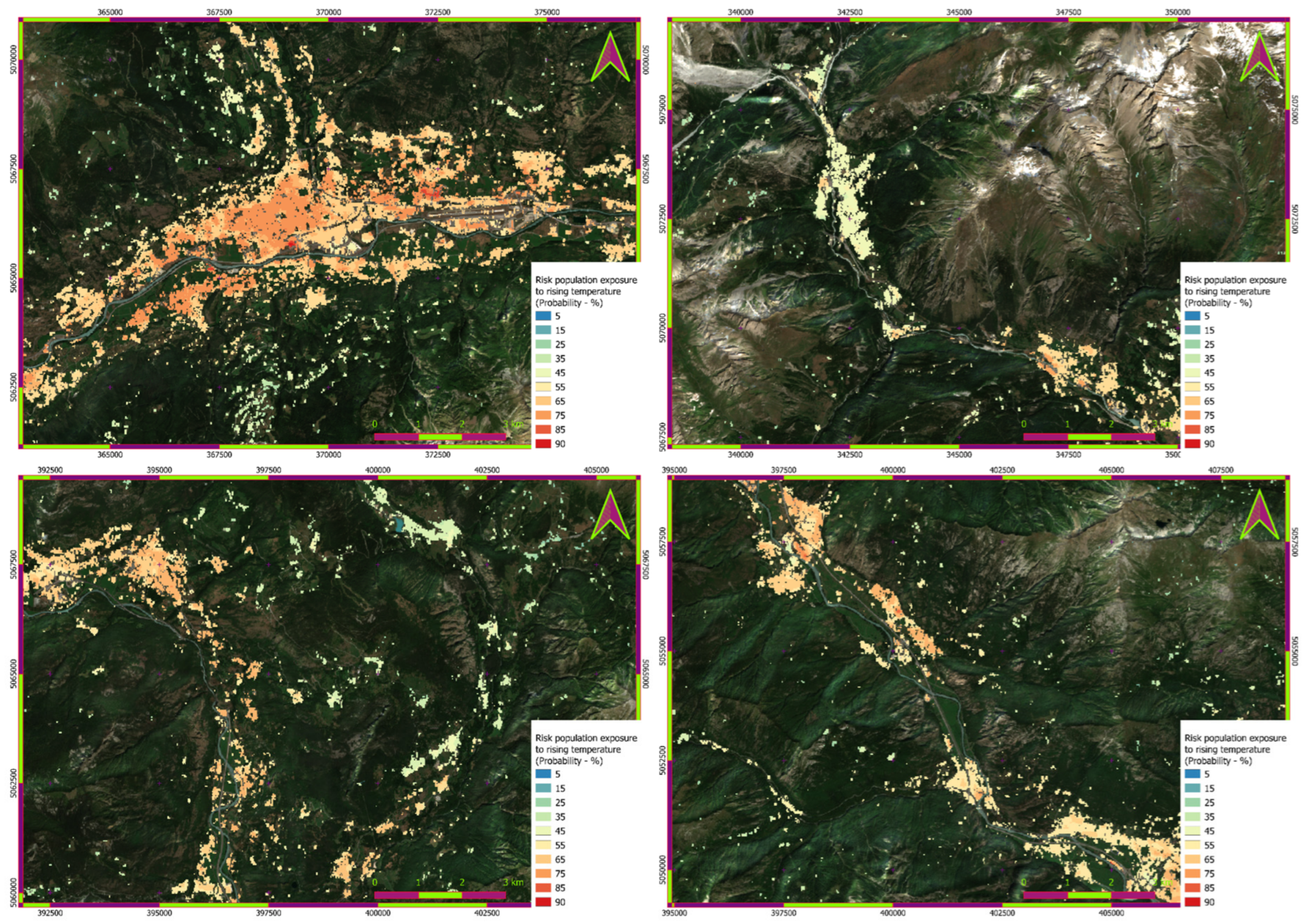
3. Result
4. Discussion
5. Conclusions
Author Contributions
Funding
Data Availability Statement
Acknowledgments
Conflicts of Interest
Appendix A

| ID Italian Municipality | Municipalities in Aosta Valley Region | HDX Meta Population 2020 (pi) | ISTAT Effective Resident on 31 December 2020 (oi) | MAE |
|---|---|---|---|---|
| A205 | Allein | 244 | 210 | 34 |
| A305 | Antey-Saint-Andre | 645 | 565 | 80 |
| A326 | Aosta | 33,204 | 33,916 | −712 |
| A424 | Arnad | 1278 | 1245 | 33 |
| A452 | Arvier | 917 | 870 | 47 |
| A521 | Avise | 378 | 306 | 72 |
| A094 | Ayas | 1406 | 1393 | 13 |
| A108 | Aymavilles | 2266 | 2104 | 162 |
| A643 | Bard | 110 | 122 | −12 |
| A877 | Bionaz | 224 | 225 | −1 |
| B192 | Brissogne | 1034 | 948 | 86 |
| B230 | Brusson | 792 | 883 | −91 |
| C593 | Challand-Saint-Anselme | 804 | 758 | 46 |
| C594 | Challand-Saint-Victor | 618 | 548 | 70 |
| C595 | Chambave | 908 | 919 | −11 |
| B491 | Chamois | 92 | 98 | −6 |
| C596 | Champdepraz | 742 | 714 | 28 |
| B540 | Champorcher | 365 | 394 | −29 |
| C598 | Charvensod | 2688 | 2338 | 350 |
| C294 | Chatillon | 5023 | 4524 | 499 |
| C821 | Cogne | 1403 | 1377 | 26 |
| D012 | Courmayeur | 2759 | 2761 | −2 |
| D338 | Donnas | 2551 | 2448 | 103 |
| D356 | Doues | 580 | 512 | 68 |
| D402 | Emarese | 247 | 223 | 24 |
| D444 | Etroubles | 539 | 481 | 58 |
| D537 | Fenis | 1860 | 1769 | 91 |
| D666 | Fontainemore | 472 | 431 | 41 |
| D839 | Gaby | 496 | 460 | 36 |
| E029 | Gignod | 2094 | 1715 | 379 |
| E165 | Gressan | 3819 | 3393 | 426 |
| E167 | Gressoney-La-Trinite | 315 | 318 | −3 |
| E168 | Gressoney-Saint-Jean | 815 | 812 | 3 |
| E273 | Hone | 1170 | 1189 | −19 |
| E306 | Introd | 696 | 661 | 35 |
| E369 | Issime | 430 | 407 | 23 |
| E371 | Issogne | 1405 | 1349 | 56 |
| E391 | Jovencan | 895 | 723 | 172 |
| A308 | La Magdeleine | 129 | 109 | 20 |
| E458 | La Salle | 2200 | 2001 | 199 |
| E470 | La Thuile | 810 | 812 | −2 |
| E587 | Lillianes | 444 | 445 | −1 |
| F367 | Montjovet | 1864 | 1802 | 62 |
| F726 | Morgex | 2166 | 2096 | 70 |
| F987 | Nus | 3228 | 2950 | 278 |
| G045 | Ollomont | 150 | 165 | −15 |
| G012 | Oyace | 223 | 217 | 6 |
| G459 | Perloz | 413 | 457 | −44 |
| G794 | Pollein | 1617 | 1536 | 81 |
| G854 | Pontboset | 185 | 173 | 12 |
| G545 | Pontey | 907 | 801 | 106 |
| G860 | Pont-Saint-Martin | 4014 | 3592 | 422 |
| H042 | Pre-Saint-Didier | 1031 | 1031 | |
| H110 | Quart | 4601 | 4045 | 556 |
| H262 | Rhemes-Notre-Dame | 111 | 85 | 26 |
| H263 | Rhemes-Saint-Georges | 192 | 174 | 18 |
| H497 | Roisan | 1217 | 1038 | 179 |
| H669 | Saint-Christophe | 3598 | 3446 | 152 |
| H670 | Saint-Denis | 399 | 382 | 17 |
| H671 | Saint-Marcel | 1385 | 1365 | 20 |
| H672 | Saint-Nicolas | 311 | 320 | −9 |
| H673 | Saint-Oyen | 240 | 199 | 41 |
| H674 | Saint-Pierre | 3512 | 3195 | 317 |
| H675 | Saint-Rhemy | 328 | 329 | −1 |
| H676 | Saint-Vincent | 4509 | 4432 | 77 |
| I442 | Sarre | 5497 | 4817 | 680 |
| L217 | Torgnon | 525 | 567 | −42 |
| L582 | Valgrisenche | 198 | 196 | 2 |
| L643 | Valpelline | 691 | 618 | 73 |
| L647 | Valsavarenche | 187 | 175 | 12 |
| L654 | Valtournenche | 2037 | 2255 | −218 |
| L783 | Verrayes | 1389 | 1264 | 125 |
| C282 | Verres | 2712 | 2577 | 135 |
| L981 | Villeneuve | 1380 | 1259 | 121 |
| Aosta Valley Region | 130,683 | 125,034 | 76 |
Appendix B
| ID Italian VDA Municipality | Cluster ID—Mean Gain LST Max—n° Population Exposed VDA General | ||||||||||
|---|---|---|---|---|---|---|---|---|---|---|---|
| I | II | III | IV | V | VI | VII | VIII | IX | X | XI | |
| A205 | 34 | 65 | 17 | 86 | 6 | 3 | 33 | ||||
| A305 | 4 | 16 | 75 | 1 | 231 | 65 | 38 | 215 | |||
| A326 | 166 | 4 | 138 | 2805 | 546 | 66 | 7 | 12,346 | 13 | 45 | 17,069 |
| A424 | 326 | 3 | 436 | 17 | 94 | 155 | 69 | 3 | 57 | 117 | |
| A452 | 12 | 9 | 534 | 171 | 4 | 186 | 1 | ||||
| A521 | 64 | 32 | 95 | 143 | 10 | 21 | 2 | 1 | 10 | ||
| A094 | 32 | 58 | 103 | 2 | 4 | 160 | 302 | 1 | 396 | 350 | |
| A108 | 32 | 26 | 529 | 122 | 11 | 1203 | 3 | 340 | |||
| A643 | 14 | 23 | 29 | 17 | 29 | ||||||
| A877 | 17 | 1 | 55 | 23 | 31 | 47 | 8 | 5 | 17 | 20 | |
| B192 | 44 | 54 | 427 | 178 | 39 | 1 | 281 | 2 | 8 | ||
| B230 | 7 | 6 | 144 | 1 | 304 | 58 | 61 | 211 | |||
| C593 | 184 | 219 | 11 | 127 | 176 | 13 | 4 | 71 | |||
| C594 | 36 | 13 | 295 | 143 | 9 | 119 | 3 | ||||
| C595 | 151 | 1 | 232 | 128 | 195 | 115 | 2 | 65 | 18 | ||
| B491 | 3 | 1 | 27 | 29 | 32 | ||||||
| C596 | 214 | 1 | 217 | 6 | 114 | 164 | 4 | 3 | 18 | ||
| B540 | 58 | 2 | 76 | 120 | 109 | ||||||
| C598 | 68 | 70 | 609 | 170 | 32 | 1476 | 1 | 263 | |||
| C294 | 785 | 6 | 1356 | 611 | 1352 | 843 | 4 | 32 | 4 | 31 | |
| C821 | 235 | 11 | 275 | 41 | 347 | 249 | 65 | 5 | 31 | 144 | |
| D012 | 224 | 161 | 1036 | 944 | 76 | 179 | 3 | 135 | |||
| D338 | 69 | 788 | 1 | 1 | 1289 | 32 | 3 | 367 | |||
| D356 | 39 | 41 | 233 | 104 | 28 | 2 | 123 | 8 | 1 | ||
| D402 | 33 | 2 | 62 | 49 | 3 | 5 | 93 | ||||
| D444 | 114 | 1 | 97 | 163 | 141 | 18 | 1 | 3 | |||
| D537 | 103 | 28 | 986 | 604 | 15 | 122 | 1 | ||||
| D666 | 38 | 9 | 105 | 3 | 193 | 24 | 18 | 82 | |||
| D839 | 4 | 84 | 238 | 40 | 8 | 122 | |||||
| E029 | 162 | 3 | 116 | 492 | 364 | 127 | 22 | 661 | 24 | 96 | 29 |
| E165 | 53 | 64 | 230 | 165 | 70 | 1 | 1723 | 25 | 1488 | ||
| E167 | 4 | 20 | 10 | 1 | 21 | 86 | 129 | 43 | 1 | ||
| E168 | 2 | 18 | 14 | 141 | 202 | 184 | 253 | ||||
| E273 | 48 | 9 | 291 | 24 | 28 | 492 | 58 | 16 | 22 | 183 | |
| E306 | 64 | 1 | 51 | 233 | 304 | 21 | 2 | 11 | 2 | 8 | |
| E369 | 15 | 22 | 36 | 3 | 150 | 32 | 55 | 116 | |||
| E371 | 344 | 25 | 326 | 10 | 411 | 154 | 41 | 31 | 63 | ||
| E391 | 40 | 502 | 352 | ||||||||
| A308 | 6 | 11 | 23 | 69 | 20 | ||||||
| E458 | 164 | 102 | 711 | 393 | 28 | 2 | 790 | 1 | 4 | 5 | |
| E470 | 34 | 27 | 364 | 240 | 3 | 142 | |||||
| E587 | 8 | 4 | 162 | 210 | 8 | 10 | 41 | ||||
| F367 | 302 | 250 | 471 | 737 | 61 | 1 | 36 | 1 | 5 | ||
| F726 | 32 | 8 | 769 | 150 | 4 | 976 | 3 | 225 | |||
| F987 | 221 | 1 | 159 | 1368 | 612 | 104 | 15 | 558 | 23 | 46 | 121 |
| G045 | 22 | 2 | 67 | 43 | 1 | 14 | 1 | ||||
| G012 | 31 | 15 | 71 | 83 | 19 | 3 | |||||
| G459 | 4 | 27 | 203 | 31 | 8 | 141 | |||||
| G794 | 15 | 3 | 575 | 102 | 3 | 1 | 871 | 2 | 44 | ||
| G854 | 3 | 37 | 67 | 7 | 72 | ||||||
| G545 | 126 | 89 | 143 | 532 | 8 | 9 | |||||
| G860 | 1017 | 3 | 1525 | 165 | 507 | 691 | 27 | 7 | 72 | ||
| H042 | 86 | 38 | 318 | 365 | 8 | 3 | 182 | 2 | 6 | 25 | |
| H110 | 220 | 2 | 208 | 1912 | 692 | 102 | 17 | 1209 | 6 | 51 | 182 |
| H262 | 18 | 18 | 1 | 7 | 32 | 2 | 32 | ||||
| H263 | 37 | 27 | 20 | 65 | 28 | 3 | 11 | ||||
| H497 | 11 | 1 | 670 | 92 | 1 | 440 | |||||
| H669 | 17 | 45 | 737 | 64 | 2 | 2340 | 391 | ||||
| H670 | 45 | 11 | 46 | 35 | 59 | 63 | 35 | 7 | 28 | 71 | |
| H671 | 69 | 1 | 79 | 651 | 226 | 28 | 4 | 308 | 3 | 10 | 6 |
| H672 | 38 | 55 | 97 | 93 | 10 | 5 | 4 | 8 | |||
| H673 | 14 | 59 | 3 | 82 | 24 | 13 | 46 | ||||
| H674 | 16 | 12 | 16 | 830 | 77 | 34 | 17 | 1773 | 17 | 21 | 700 |
| H675 | 29 | 37 | 24 | 40 | 140 | 2 | 12 | 41 | 3 | ||
| H676 | 801 | 3 | 403 | 884 | 2068 | 117 | 34 | 93 | 22 | 83 | |
| I442 | 178 | 1 | 128 | 1655 | 358 | 139 | 4 | 2338 | 16 | 42 | 640 |
| L217 | 56 | 6 | 28 | 141 | 134 | 159 | |||||
| L582 | 35 | 15 | 49 | 87 | 4 | 4 | 2 | 2 | |||
| L643 | 94 | 87 | 202 | 185 | 22 | 1 | 93 | 6 | 2 | ||
| L647 | 51 | 1 | 21 | 19 | 46 | 29 | 1 | 2 | 1 | 16 | |
| L654 | 81 | 73 | 426 | 381 | 358 | 717 | |||||
| L783 | 191 | 8 | 242 | 75 | 234 | 310 | 95 | 7 | 43 | 184 | |
| C282 | 714 | 1 | 591 | 394 | 449 | 265 | 3 | 167 | 2 | 91 | 35 |
| L981 | 70 | 40 | 475 | 198 | 9 | 1 | 553 | 1 | 34 | ||
| VDA overall | 8443 | 480 | 10,420 | 23,334 | 15,635 | 9077 | 2235 | 31,980 | 2033 | 4946 | 22,101 |
| VDA overall % | 6.5 | 0.4 | 8.0 | 17.9 | 12.0 | 6.9 | 1.7 | 24.5 | 1.6 | 3.8 | 16.9 |
| ID Italian VDA Municipality | Cluster ID—Mean Gain LST Max—n° Population Exposed VDA Men | ||||||||||
| I | II | III | IV | V | VI | VII | VIII | IX | X | XI | |
| A205 | 17 | 33 | 6 | 46 | 3 | 1 | 16 | ||||
| A305 | 2 | 9 | 34 | 114 | 32 | 19 | 105 | ||||
| A326 | 86 | 2 | 72 | 1381 | 274 | 35 | 4 | 5852 | 7 | 23 | 7704 |
| A424 | 155 | 1 | 203 | 8 | 43 | 73 | 34 | 1 | 29 | 56 | |
| A452 | 6 | 4 | 273 | 84 | 2 | 96 | 1 | ||||
| A521 | 31 | 16 | 45 | 69 | 6 | 10 | 1 | 1 | 5 | ||
| A094 | 17 | 31 | 54 | 1 | 2 | 80 | 154 | 194 | 174 | ||
| A108 | 16 | 12 | 262 | 61 | 5 | 597 | 1 | 168 | |||
| A643 | 6 | 11 | 13 | 8 | 13 | ||||||
| A877 | 9 | 29 | 12 | 16 | 27 | 4 | 2 | 7 | 12 | ||
| B192 | 26 | 28 | 218 | 92 | 21 | 144 | 1 | 4 | |||
| B230 | 4 | 4 | 70 | 142 | 29 | 30 | 98 | ||||
| C593 | 90 | 107 | 6 | 63 | 90 | 7 | 2 | 38 | |||
| C594 | 18 | 7 | 147 | 73 | 5 | 61 | 2 | ||||
| C595 | 75 | 1 | 113 | 67 | 99 | 56 | 1 | 34 | 10 | ||
| B491 | 2 | 1 | 13 | 14 | 15 | ||||||
| C596 | 100 | 1 | 103 | 3 | 57 | 79 | 2 | 2 | 9 | ||
| B540 | 27 | 1 | 37 | 59 | 56 | ||||||
| C598 | 35 | 37 | 303 | 86 | 17 | 731 | 131 | ||||
| C294 | 375 | 3 | 658 | 303 | 656 | 413 | 2 | 15 | 2 | 15 | |
| C821 | 115 | 5 | 135 | 20 | 177 | 123 | 33 | 2 | 15 | 70 | |
| D012 | 113 | 84 | 510 | 468 | 40 | 90 | 1 | 71 | |||
| D338 | 33 | 371 | 1 | 615 | 16 | 2 | 179 | ||||
| D356 | 19 | 20 | 114 | 51 | 14 | 1 | 58 | 4 | 1 | ||
| D402 | 15 | 1 | 33 | 26 | 2 | 2 | 53 | ||||
| D444 | 58 | 1 | 49 | 83 | 71 | 9 | 2 | ||||
| D537 | 51 | 14 | 500 | 297 | 7 | 63 | 1 | ||||
| D666 | 20 | 5 | 53 | 2 | 97 | 13 | 10 | 42 | |||
| D839 | 2 | 42 | 115 | 21 | 4 | 58 | |||||
| E029 | 78 | 1 | 60 | 233 | 175 | 68 | 12 | 326 | 12 | 50 | 15 |
| E165 | 29 | 34 | 116 | 89 | 36 | 859 | 12 | 735 | |||
| E167 | 2 | 8 | 5 | 10 | 40 | 56 | 21 | 1 | |||
| E168 | 1 | 8 | 6 | 68 | 100 | 90 | 125 | ||||
| E273 | 24 | 4 | 137 | 11 | 14 | 234 | 27 | 8 | 11 | 87 | |
| E306 | 32 | 26 | 119 | 147 | 10 | 1 | 6 | 1 | 4 | ||
| E369 | 8 | 12 | 18 | 1 | 72 | 16 | 28 | 57 | |||
| E371 | 167 | 12 | 157 | 5 | 203 | 74 | 20 | 15 | 29 | ||
| E391 | 21 | 255 | 181 | ||||||||
| A308 | 3 | 6 | 13 | 36 | 12 | ||||||
| E458 | 82 | 50 | 352 | 199 | 14 | 1 | 386 | 2 | 2 | ||
| E470 | 18 | 14 | 179 | 119 | 2 | 70 | |||||
| E587 | 4 | 2 | 74 | 99 | 5 | 5 | 21 | ||||
| F367 | 156 | 131 | 239 | 381 | 31 | 1 | 18 | 3 | |||
| F726 | 17 | 4 | 378 | 70 | 2 | 474 | 1 | 105 | |||
| F987 | 111 | 82 | 662 | 302 | 52 | 8 | 270 | 13 | 24 | 60 | |
| G045 | 10 | 1 | 36 | 21 | 8 | ||||||
| G012 | 16 | 9 | 37 | 46 | 13 | 2 | |||||
| G459 | 2 | 12 | 96 | 18 | 5 | 70 | |||||
| G794 | 8 | 2 | 289 | 52 | 2 | 1 | 434 | 1 | 22 | ||
| G854 | 2 | 17 | 35 | 4 | 34 | ||||||
| G545 | 62 | 43 | 69 | 266 | 4 | 5 | |||||
| G860 | 497 | 2 | 740 | 78 | 244 | 335 | 14 | 4 | 39 | ||
| H042 | 43 | 18 | 167 | 187 | 4 | 2 | 94 | 1 | 3 | 12 | |
| H110 | 113 | 1 | 108 | 958 | 347 | 53 | 9 | 606 | 4 | 27 | 98 |
| H262 | 10 | 9 | 1 | 4 | 20 | 1 | 21 | ||||
| H263 | 18 | 13 | 10 | 32 | 14 | 2 | 6 | ||||
| H497 | 5 | 337 | 46 | 218 | |||||||
| H669 | 8 | 22 | 361 | 31 | 1 | 1149 | 193 | ||||
| H670 | 22 | 6 | 23 | 18 | 29 | 33 | 18 | 4 | 16 | 38 | |
| H671 | 34 | 39 | 319 | 112 | 14 | 2 | 151 | 2 | 6 | 3 | |
| H672 | 18 | 31 | 49 | 44 | 5 | 3 | 2 | 4 | |||
| H673 | 7 | 28 | 1 | 39 | 11 | 6 | 22 | ||||
| H674 | 8 | 6 | 8 | 412 | 38 | 18 | 9 | 889 | 9 | 10 | 350 |
| H675 | 16 | 20 | 12 | 20 | 77 | 1 | 6 | 23 | 2 | ||
| H676 | 396 | 2 | 203 | 429 | 995 | 61 | 18 | 46 | 10 | 42 | |
| I442 | 89 | 1 | 64 | 801 | 180 | 70 | 2 | 1148 | 13 | 20 | 316 |
| L217 | 27 | 3 | 15 | 75 | 70 | 82 | |||||
| L582 | 18 | 8 | 24 | 46 | 3 | 2 | 1 | 1 | |||
| L643 | 50 | 46 | 107 | 98 | 11 | 50 | 3 | 1 | |||
| L647 | 23 | 10 | 9 | 20 | 15 | 1 | 1 | 9 | |||
| L654 | 38 | 37 | 217 | 201 | 184 | 380 | |||||
| L783 | 98 | 4 | 125 | 39 | 120 | 158 | 47 | 4 | 21 | 90 | |
| C282 | 346 | 1 | 286 | 195 | 217 | 126 | 2 | 82 | 1 | 43 | 17 |
| L981 | 36 | 20 | 246 | 100 | 5 | 1 | 281 | 1 | 17 | ||
| VDA overall | 4172 | 237 | 5118 | 11,574 | 7744 | 4476 | 1141 | 15,594 | 1019 | 2490 | 10,210 |
| VDA overall % | 6.5 | 0.4 | 8.0 | 18.1 | 12.1 | 7.0 | 1.8 | 24.5 | 1.6 | 3.9 | 16.0 |
| ID Italian VDA Municipality | Cluster ID—Mean Gain LST Max—n° Population Exposed VDA Women | ||||||||||
| I | II | III | IV | V | VI | VII | VIII | IX | X | XI | |
| A205 | 17 | 32 | 10 | 41 | 3 | 2 | 17 | ||||
| A305 | 2 | 7 | 40 | 1 | 117 | 33 | 19 | 110 | |||
| A326 | 80 | 2 | 66 | 1423 | 273 | 31 | 3 | 6493 | 6 | 21 | 9365 |
| A424 | 172 | 2 | 233 | 9 | 50 | 82 | 35 | 1 | 29 | 61 | |
| A452 | 6 | 5 | 261 | 88 | 2 | 90 | 1 | ||||
| A521 | 33 | 16 | 49 | 73 | 4 | 11 | 1 | 5 | |||
| A094 | 15 | 27 | 49 | 1 | 2 | 79 | 148 | 201 | 176 | ||
| A108 | 16 | 14 | 267 | 61 | 6 | 606 | 2 | 173 | |||
| A643 | 7 | 12 | 15 | 9 | 15 | ||||||
| A877 | 8 | 26 | 11 | 15 | 20 | 4 | 3 | 10 | 8 | ||
| B192 | 18 | 26 | 209 | 85 | 17 | 137 | 1 | 4 | |||
| B230 | 4 | 3 | 74 | 161 | 29 | 30 | 112 | ||||
| C593 | 94 | 112 | 5 | 63 | 86 | 6 | 2 | 32 | |||
| C594 | 18 | 6 | 148 | 70 | 4 | 58 | 1 | ||||
| C595 | 75 | 1 | 119 | 61 | 96 | 59 | 1 | 31 | 9 | ||
| B491 | 1 | 1 | 14 | 15 | 17 | ||||||
| C596 | 114 | 1 | 114 | 3 | 57 | 85 | 2 | 1 | 9 | ||
| B540 | 31 | 1 | 39 | 61 | 53 | ||||||
| C598 | 32 | 33 | 306 | 83 | 15 | 746 | 132 | ||||
| C294 | 410 | 3 | 698 | 308 | 695 | 431 | 2 | 17 | 2 | 15 | |
| C821 | 121 | 5 | 140 | 20 | 170 | 126 | 32 | 2 | 16 | 74 | |
| D012 | 111 | 77 | 526 | 477 | 36 | 90 | 1 | 64 | |||
| D338 | 36 | 417 | 1 | 674 | 15 | 1 | 187 | ||||
| D356 | 20 | 21 | 119 | 53 | 14 | 1 | 65 | 4 | |||
| D402 | 19 | 1 | 29 | 23 | 1 | 2 | 39 | ||||
| D444 | 56 | 1 | 48 | 81 | 70 | 9 | 2 | ||||
| D537 | 53 | 14 | 486 | 307 | 8 | 59 | 1 | ||||
| D666 | 18 | 4 | 53 | 2 | 95 | 11 | 8 | 40 | |||
| D839 | 2 | 43 | 124 | 18 | 3 | 64 | |||||
| E029 | 83 | 2 | 56 | 259 | 189 | 59 | 10 | 335 | 12 | 46 | 14 |
| E165 | 24 | 29 | 114 | 77 | 34 | 1 | 864 | 12 | 753 | ||
| E167 | 2 | 12 | 5 | 11 | 46 | 73 | 22 | 1 | |||
| E168 | 1 | 11 | 8 | 73 | 102 | 94 | 128 | ||||
| E273 | 25 | 5 | 154 | 12 | 14 | 257 | 30 | 8 | 11 | 96 | |
| E306 | 32 | 26 | 114 | 157 | 11 | 1 | 5 | 1 | 4 | ||
| E369 | 8 | 10 | 18 | 1 | 78 | 16 | 26 | 59 | |||
| E371 | 177 | 13 | 169 | 5 | 208 | 80 | 21 | 16 | 34 | ||
| E391 | 20 | 247 | 171 | ||||||||
| A308 | 3 | 4 | 10 | 33 | 9 | ||||||
| E458 | 82 | 51 | 359 | 194 | 14 | 1 | 405 | 2 | 3 | ||
| E470 | 17 | 13 | 184 | 121 | 1 | 72 | |||||
| E587 | 5 | 2 | 87 | 111 | 3 | 5 | 20 | ||||
| F367 | 146 | 120 | 232 | 355 | 29 | 1 | 17 | 3 | |||
| F726 | 15 | 4 | 391 | 80 | 2 | 502 | 2 | 120 | |||
| F987 | 109 | 77 | 706 | 311 | 51 | 7 | 289 | 9 | 22 | 60 | |
| G045 | 12 | 1 | 32 | 22 | 5 | ||||||
| G012 | 14 | 7 | 34 | 37 | 6 | 1 | |||||
| G459 | 1 | 14 | 107 | 13 | 3 | 71 | |||||
| G794 | 7 | 1 | 287 | 50 | 2 | 1 | 437 | 1 | 22 | ||
| G854 | 1 | 20 | 32 | 2 | 38 | ||||||
| G545 | 64 | 46 | 75 | 266 | 4 | 4 | |||||
| G860 | 521 | 1 | 785 | 87 | 263 | 356 | 13 | 3 | 32 | ||
| H042 | 43 | 20 | 151 | 178 | 4 | 2 | 87 | 1 | 3 | 13 | |
| H110 | 107 | 1 | 100 | 954 | 345 | 49 | 8 | 602 | 2 | 24 | 84 |
| H262 | 8 | 9 | 3 | 13 | 1 | 11 | |||||
| H263 | 19 | 14 | 10 | 33 | 14 | 1 | 5 | ||||
| H497 | 6 | 1 | 333 | 46 | 1 | 222 | |||||
| H669 | 9 | 24 | 376 | 33 | 1 | 1192 | 198 | ||||
| H670 | 22 | 5 | 23 | 17 | 30 | 30 | 17 | 4 | 12 | 33 | |
| H671 | 35 | 40 | 332 | 113 | 14 | 2 | 156 | 1 | 4 | 3 | |
| H672 | 20 | 24 | 49 | 50 | 5 | 2 | 2 | 4 | |||
| H673 | 7 | 31 | 1 | 43 | 13 | 7 | 24 | ||||
| H674 | 9 | 5 | 9 | 418 | 38 | 16 | 8 | 883 | 8 | 11 | 350 |
| H675 | 13 | 17 | 12 | 20 | 63 | 1 | 6 | 19 | 2 | ||
| H676 | 405 | 2 | 200 | 456 | 1073 | 57 | 16 | 46 | 12 | 40 | |
| I442 | 89 | 63 | 854 | 179 | 68 | 1 | 1190 | 3 | 22 | 323 | |
| L217 | 29 | 3 | 14 | 66 | 65 | 77 | |||||
| L582 | 17 | 7 | 24 | 41 | 1 | 1 | 1 | ||||
| L643 | 44 | 41 | 95 | 86 | 11 | 43 | 3 | 1 | |||
| L647 | 28 | 11 | 10 | 26 | 14 | 1 | 7 | ||||
| L654 | 44 | 36 | 209 | 180 | 174 | 337 | |||||
| L783 | 93 | 4 | 116 | 37 | 114 | 152 | 48 | 3 | 22 | 94 | |
| C282 | 368 | 1 | 305 | 199 | 232 | 139 | 1 | 85 | 1 | 48 | 18 |
| L981 | 34 | 20 | 230 | 98 | 3 | 271 | 17 | ||||
| VDA overall | 4274 | 244 | 5304 | 11,763 | 7890 | 4597 | 1094 | 16,384 | 1008 | 2451 | 11,892 |
| VDA overall % | 6.4 | 0.4 | 7.9 | 17.6 | 11.8 | 6.9 | 1.6 | 24.5 | 1.5 | 3.7 | 17.8 |
| ID Italian VDA Municipality | Cluster ID—Mean Gain LST Max—n° Population Exposed VDA Women of Reproductive Age 15–49 | ||||||||||
| I | II | III | IV | V | VI | VII | VIII | IX | X | XI | |
| A205 | 8 | 13 | 7 | 12 | 1 | 4 | |||||
| A305 | 1 | 3 | 18 | 51 | 14 | 9 | 51 | ||||
| A326 | 36 | 1 | 30 | 610 | 121 | 15 | 2 | 2504 | 3 | 10 | 3690 |
| A424 | 70 | 1 | 97 | 4 | 22 | 33 | 14 | 1 | 11 | 25 | |
| A452 | 3 | 2 | 124 | 39 | 1 | 45 | |||||
| A521 | 13 | 6 | 19 | 29 | 1 | 5 | 2 | ||||
| A094 | 9 | 11 | 26 | 1 | 1 | 36 | 65 | 76 | 76 | ||
| A108 | 6 | 6 | 121 | 26 | 4 | 282 | 1 | 81 | |||
| A643 | 3 | 5 | 6 | 3 | 6 | ||||||
| A877 | 4 | 12 | 5 | 7 | 9 | 2 | 1 | 4 | 4 | ||
| B192 | 8 | 11 | 95 | 40 | 7 | 62 | 1 | ||||
| B230 | 2 | 1 | 32 | 66 | 12 | 10 | 44 | ||||
| C593 | 43 | 50 | 2 | 31 | 37 | 3 | 1 | 14 | |||
| C594 | 6 | 3 | 74 | 28 | 2 | 28 | 1 | ||||
| C595 | 30 | 48 | 26 | 39 | 25 | 15 | 4 | ||||
| B491 | 5 | 5 | 7 | ||||||||
| C596 | 53 | 50 | 2 | 30 | 37 | 1 | 1 | 4 | |||
| B540 | 14 | 17 | 29 | 22 | |||||||
| C598 | 17 | 18 | 143 | 42 | 9 | 349 | 62 | ||||
| C294 | 183 | 2 | 304 | 136 | 309 | 182 | 1 | 8 | 1 | 7 | |
| C821 | 48 | 2 | 58 | 7 | 69 | 53 | 12 | 1 | 6 | 30 | |
| D012 | 51 | 35 | 238 | 214 | 16 | 44 | 1 | 33 | |||
| D338 | 16 | 173 | 283 | 7 | 1 | 81 | |||||
| D356 | 8 | 10 | 46 | 20 | 7 | 32 | 1 | ||||
| D402 | 10 | 1 | 14 | 9 | 1 | 1 | 17 | ||||
| D444 | 25 | 20 | 38 | 32 | 2 | 1 | |||||
| D537 | 23 | 6 | 211 | 132 | 3 | 26 | |||||
| D666 | 8 | 2 | 22 | 1 | 36 | 4 | 3 | 15 | |||
| D839 | 1 | 15 | 43 | 10 | 1 | 24 | |||||
| E029 | 39 | 1 | 26 | 125 | 89 | 30 | 6 | 165 | 7 | 25 | 7 |
| E165 | 14 | 17 | 57 | 41 | 20 | 383 | 7 | 343 | |||
| E167 | 1 | 6 | 2 | 5 | 20 | 32 | 10 | ||||
| E168 | 1 | 4 | 4 | 33 | 44 | 42 | 55 | ||||
| E273 | 11 | 2 | 76 | 5 | 6 | 118 | 13 | 4 | 5 | 41 | |
| E306 | 16 | 12 | 49 | 71 | 5 | 1 | 2 | 1 | 2 | ||
| E369 | 3 | 4 | 7 | 1 | 31 | 6 | 11 | 24 | |||
| E371 | 67 | 5 | 65 | 2 | 79 | 35 | 11 | 6 | 15 | ||
| E391 | 10 | 129 | 86 | ||||||||
| A308 | 1 | 2 | 5 | 15 | 4 | ||||||
| E458 | 32 | 20 | 162 | 84 | 6 | 173 | 1 | 1 | |||
| E470 | 7 | 6 | 76 | 53 | 1 | 31 | |||||
| E587 | 2 | 1 | 34 | 47 | 2 | 2 | 9 | ||||
| F367 | 69 | 55 | 108 | 162 | 15 | 1 | 8 | 2 | |||
| F726 | 8 | 2 | 175 | 36 | 1 | 226 | 1 | 54 | |||
| F987 | 48 | 34 | 337 | 139 | 21 | 2 | 139 | 3 | 8 | 28 | |
| G045 | 5 | 14 | 11 | 2 | |||||||
| G012 | 7 | 3 | 17 | 16 | 3 | 1 | |||||
| G459 | 7 | 49 | 3 | 31 | |||||||
| G794 | 3 | 1 | 135 | 23 | 1 | 205 | 10 | ||||
| G854 | 1 | 7 | 12 | 1 | 14 | ||||||
| G545 | 31 | 22 | 36 | 129 | 2 | 1 | |||||
| G860 | 231 | 1 | 330 | 40 | 118 | 147 | 5 | 1 | 14 | ||
| H042 | 20 | 9 | 73 | 82 | 2 | 1 | 45 | 2 | 7 | ||
| H110 | 50 | 44 | 458 | 164 | 21 | 3 | 291 | 1 | 11 | 38 | |
| H262 | 4 | 4 | 1 | 6 | 4 | ||||||
| H263 | 6 | 6 | 4 | 12 | 7 | 1 | 2 | ||||
| H497 | 3 | 161 | 23 | 104 | |||||||
| H669 | 4 | 11 | 173 | 16 | 1 | 525 | 92 | ||||
| H670 | 11 | 3 | 13 | 9 | 13 | 12 | 9 | 2 | 7 | 16 | |
| H671 | 15 | 18 | 148 | 51 | 6 | 1 | 68 | 1 | 2 | 1 | |
| H672 | 8 | 14 | 22 | 22 | 2 | 1 | 1 | 1 | |||
| H673 | 3 | 13 | 1 | 18 | 5 | 3 | 10 | ||||
| H674 | 5 | 2 | 5 | 195 | 20 | 7 | 4 | 420 | 4 | 6 | 166 |
| H675 | 6 | 7 | 5 | 8 | 27 | 2 | 8 | ||||
| H676 | 171 | 1 | 88 | 195 | 431 | 26 | 7 | 22 | 4 | 18 | |
| I442 | 41 | 26 | 411 | 83 | 29 | 1 | 567 | 1 | 11 | 147 | |
| L217 | 12 | 2 | 8 | 29 | 28 | 34 | |||||
| L582 | 7 | 3 | 7 | 14 | 1 | ||||||
| L643 | 19 | 18 | 46 | 40 | 5 | 20 | 1 | ||||
| L647 | 12 | 4 | 4 | 11 | 7 | 4 | |||||
| L654 | 20 | 16 | 92 | 84 | 78 | 156 | |||||
| L783 | 40 | 1 | 50 | 16 | 47 | 62 | 18 | 2 | 7 | 39 | |
| C282 | 147 | 122 | 81 | 89 | 56 | 38 | 18 | 7 | |||
| L981 | 16 | 10 | 102 | 45 | 2 | 123 | 7 | ||||
| VDA overall | 1866 | 106 | 2291 | 5360 | 3468 | 1958 | 475 | 7095 | 427 | 1062 | 4862 |
| VDA overall % | 6.4 | 0.4 | 7.9 | 18.5 | 12.0 | 6.8 | 1.6 | 24.5 | 1.5 | 3.7 | 16.8 |
| ID Italian VDA Municipality | Cluster ID—Mean Gain LST Max—n° Population Exposed VDA Elderly 60 Plus | ||||||||||
| I | II | III | IV | V | VI | VII | VIII | IX | X | XI | |
| A205 | 10 | 19 | 1 | 35 | 3 | 1 | 13 | ||||
| A305 | 1 | 3 | 21 | 61 | 18 | 10 | 55 | ||||
| A326 | 39 | 1 | 31 | 775 | 143 | 14 | 1 | 4048 | 2 | 9 | 5644 |
| A424 | 102 | 1 | 131 | 5 | 26 | 44 | 17 | 1 | 14 | 30 | |
| A452 | 5 | 5 | 125 | 48 | 2 | 41 | 1 | ||||
| A521 | 16 | 8 | 19 | 33 | 3 | 3 | 1 | 2 | |||
| A094 | 8 | 18 | 27 | 1 | 38 | 73 | 106 | 88 | |||
| A108 | 9 | 6 | 130 | 34 | 2 | 306 | 1 | 88 | |||
| A643 | 5 | 9 | 11 | 6 | 11 | ||||||
| A877 | 4 | 14 | 6 | 8 | 11 | 3 | 1 | 6 | 4 | ||
| B192 | 8 | 14 | 96 | 38 | 11 | 62 | 1 | 2 | |||
| B230 | 2 | 2 | 37 | 84 | 17 | 20 | 65 | ||||
| C593 | 51 | 69 | 4 | 32 | 54 | 4 | 2 | 24 | |||
| C594 | 13 | 3 | 76 | 47 | 3 | 34 | 1 | ||||
| C595 | 46 | 1 | 71 | 35 | 57 | 36 | 1 | 16 | 6 | ||
| B491 | 1 | 1 | 10 | 11 | 11 | ||||||
| C596 | 48 | 55 | 1 | 23 | 44 | 1 | 5 | ||||
| B540 | 19 | 1 | 28 | 40 | 38 | ||||||
| C598 | 13 | 12 | 138 | 35 | 5 | 333 | 58 | ||||
| C294 | 223 | 1 | 376 | 168 | 381 | 247 | 6 | 5 | |||
| C821 | 80 | 3 | 90 | 15 | 119 | 82 | 21 | 1 | 11 | 49 | |
| D012 | 57 | 43 | 263 | 254 | 21 | 37 | 1 | 27 | |||
| D338 | 18 | 231 | 372 | 9 | 1 | 104 | |||||
| D356 | 11 | 12 | 71 | 30 | 8 | 1 | 31 | 5 | |||
| D402 | 9 | 16 | 16 | 1 | 1 | 30 | |||||
| D444 | 28 | 25 | 43 | 39 | 7 | 2 | |||||
| D537 | 29 | 8 | 251 | 161 | 4 | 30 | |||||
| D666 | 13 | 3 | 36 | 1 | 63 | 8 | 5 | 28 | |||
| D839 | 3 | 29 | 86 | 9 | 6 | 42 | |||||
| E029 | 35 | 23 | 102 | 78 | 26 | 3 | 133 | 3 | 17 | 6 | |
| E165 | 9 | 12 | 53 | 30 | 14 | 463 | 5 | 354 | |||
| E167 | 1 | 4 | 3 | 6 | 20 | 28 | 8 | ||||
| E168 | 1 | 4 | 4 | 40 | 59 | 47 | 75 | ||||
| E273 | 14 | 2 | 80 | 7 | 8 | 143 | 17 | 5 | 6 | 55 | |
| E306 | 15 | 12 | 59 | 75 | 5 | 3 | 2 | ||||
| E369 | 3 | 6 | 8 | 1 | 45 | 10 | 16 | 38 | |||
| E371 | 104 | 8 | 97 | 3 | 128 | 44 | 10 | 9 | 19 | ||
| E391 | 8 | 101 | 71 | ||||||||
| A308 | 1 | 3 | 7 | 18 | 6 | ||||||
| E458 | 42 | 24 | 172 | 104 | 8 | 196 | 1 | 2 | |||
| E470 | 8 | 7 | 89 | 56 | 1 | 38 | |||||
| E587 | 3 | 1 | 54 | 67 | 3 | 3 | 13 | ||||
| F367 | 71 | 60 | 105 | 185 | 13 | 8 | 1 | ||||
| F726 | 4 | 1 | 200 | 37 | 1 | 242 | 55 | ||||
| F987 | 53 | 39 | 292 | 137 | 29 | 4 | 115 | 7 | 12 | 26 | |
| G045 | 7 | 1 | 20 | 14 | 3 | ||||||
| G012 | 7 | 4 | 13 | 17 | 5 | 1 | |||||
| G459 | 2 | 7 | 56 | 14 | 4 | 43 | |||||
| G794 | 4 | 1 | 133 | 25 | 1 | 193 | 1 | 10 | |||
| G854 | 14 | 25 | 1 | 25 | |||||||
| G545 | 29 | 21 | 34 | 122 | 2 | 2 | |||||
| G860 | 288 | 440 | 48 | 147 | 198 | 7 | 2 | 21 | |||
| H042 | 23 | 11 | 79 | 98 | 1 | 43 | 1 | 1 | 6 | ||
| H110 | 49 | 1 | 49 | 431 | 158 | 26 | 5 | 273 | 4 | 14 | 43 |
| H262 | 3 | 3 | 1 | 8 | 1 | 9 | |||||
| H263 | 15 | 6 | 7 | 24 | 5 | 1 | 2 | ||||
| H497 | 2 | 149 | 19 | 100 | |||||||
| H669 | 4 | 10 | 186 | 16 | 1 | 610 | 102 | ||||
| H670 | 12 | 3 | 9 | 7 | 15 | 18 | 9 | 2 | 5 | 19 | |
| H671 | 20 | 22 | 171 | 58 | 10 | 85 | 3 | 2 | |||
| H672 | 10 | 10 | 26 | 24 | 3 | 2 | 1 | 2 | |||
| H673 | 4 | 17 | 1 | 24 | 7 | 4 | 13 | ||||
| H674 | 4 | 3 | 3 | 206 | 20 | 11 | 4 | 418 | 4 | 4 | 167 |
| H675 | 8 | 11 | 6 | 12 | 41 | 4 | 12 | 1 | |||
| H676 | 234 | 114 | 265 | 646 | 31 | 5 | 24 | 4 | 20 | ||
| I442 | 44 | 34 | 389 | 87 | 35 | 1 | 565 | 5 | 8 | 165 | |
| L217 | 17 | 2 | 9 | 41 | 41 | 50 | |||||
| L582 | 11 | 5 | 16 | 29 | 1 | 1 | 1 | ||||
| L643 | 25 | 24 | 49 | 47 | 5 | 24 | 1 | ||||
| L647 | 14 | 9 | 6 | 14 | 9 | 1 | 3 | ||||
| L654 | 20 | 20 | 119 | 87 | 87 | 160 | |||||
| L783 | 51 | 2 | 68 | 22 | 64 | 95 | 31 | 2 | 15 | 59 | |
| C282 | 204 | 1 | 168 | 123 | 150 | 75 | 2 | 44 | 1 | 26 | 11 |
| L981 | 18 | 8 | 116 | 52 | 2 | 130 | 9 | ||||
| VDA overall | 2299 | 135 | 2901 | 5816 | 4210 | 2613 | 611 | 8772 | 553 | 1383 | 6851 |
| VDA overall % | 6.4 | 0.4 | 8.0 | 16.1 | 11.6 | 7.2 | 1.7 | 24.3 | 1.5 | 3.8 | 19.0 |
| ID Italian VDA Municipality | Cluster ID—Mean Gain LST Max—n° Population Exposed Children under 5 | ||||||||||
| I | II | III | IV | V | VI | VII | VIII | IX | X | XI | |
| A205 | 2 | 6 | 1 | 4 | 3 | ||||||
| A305 | 2 | 3 | 12 | 5 | 2 | 14 | |||||
| A326 | 9 | 10 | 127 | 27 | 3 | 520 | 1 | 2 | 732 | ||
| A424 | 15 | 20 | 1 | 4 | 6 | 3 | 2 | 6 | |||
| A452 | 29 | 8 | 11 | ||||||||
| A521 | 5 | 3 | 10 | 13 | 1 | 3 | 2 | ||||
| A094 | 2 | 5 | 8 | 12 | 15 | 29 | 21 | ||||
| A108 | 1 | 27 | 5 | 57 | 16 | ||||||
| A643 | 1 | 1 | 1 | 1 | |||||||
| A877 | 1 | 3 | 1 | 2 | 2 | 1 | 1 | 1 | |||
| B192 | 1 | 2 | 19 | 8 | 13 | ||||||
| B230 | 10 | 15 | 2 | 3 | 9 | ||||||
| C593 | 8 | 9 | 8 | 9 | 4 | ||||||
| C594 | 1 | 15 | 5 | 1 | 6 | ||||||
| C595 | 7 | 9 | 5 | 9 | 4 | 2 | 1 | ||||
| B491 | 1 | 1 | 1 | ||||||||
| C596 | 9 | 9 | 6 | 7 | 1 | ||||||
| B540 | 1 | 2 | 5 | 3 | |||||||
| C598 | 4 | 4 | 34 | 10 | 2 | 82 | 14 | ||||
| C294 | 39 | 1 | 70 | 33 | 76 | 32 | 2 | 1 | |||
| C821 | 9 | 11 | 1 | 12 | 9 | 2 | 1 | 4 | |||
| D012 | 9 | 5 | 50 | 44 | 2 | 8 | 8 | ||||
| D338 | 3 | 34 | 66 | 1 | 19 | ||||||
| D356 | 2 | 2 | 10 | 4 | 2 | 8 | |||||
| D402 | 1 | 3 | 4 | 6 | |||||||
| D444 | 7 | 7 | 6 | 6 | 1 | ||||||
| D537 | 5 | 2 | 56 | 30 | 1 | 8 | |||||
| D666 | 1 | 4 | 9 | 1 | 1 | 4 | |||||
| D839 | 2 | 8 | 3 | 4 | |||||||
| E029 | 8 | 7 | 31 | 21 | 8 | 1 | 45 | 1 | 5 | 2 | |
| E165 | 2 | 2 | 11 | 7 | 3 | 87 | 1 | 91 | |||
| E167 | 2 | 1 | 1 | 7 | 10 | 4 | |||||
| E168 | 2 | 1 | 8 | 7 | 9 | 10 | |||||
| E273 | 2 | 1 | 7 | 1 | 1 | 17 | 3 | 1 | 1 | 8 | |
| E306 | 4 | 4 | 16 | 20 | 1 | 1 | 1 | ||||
| E369 | 1 | 1 | 2 | 10 | 2 | 4 | 6 | ||||
| E371 | 17 | 2 | 17 | 19 | 8 | 3 | 2 | 4 | |||
| E391 | 2 | 28 | 20 | ||||||||
| A308 | 1 | 1 | 3 | 1 | |||||||
| E458 | 11 | 7 | 41 | 23 | 1 | 49 | |||||
| E470 | 1 | 1 | 16 | 10 | 7 | ||||||
| E587 | 5 | 7 | 1 | 1 | 2 | ||||||
| F367 | 12 | 12 | 23 | 35 | 3 | 2 | |||||
| F726 | 3 | 1 | 39 | 9 | 48 | 10 | |||||
| F987 | 12 | 8 | 76 | 31 | 3 | 1 | 31 | 1 | 1 | 7 | |
| G045 | 1 | 2 | 2 | ||||||||
| G012 | 2 | 1 | 5 | 5 | 1 | ||||||
| G459 | 1 | 8 | 1 | 7 | |||||||
| G794 | 1 | 27 | 4 | 48 | 2 | ||||||
| G854 | 3 | 4 | |||||||||
| G545 | 4 | 3 | 4 | 20 | |||||||
| G860 | 50 | 69 | 8 | 24 | 31 | 1 | 1 | ||||
| H042 | 5 | 2 | 16 | 18 | 1 | 9 | 1 | 1 | |||
| H110 | 12 | 10 | 114 | 40 | 5 | 1 | 70 | 2 | 9 | ||
| H262 | 1 | 1 | 3 | 3 | |||||||
| H263 | 1 | 2 | 1 | 2 | 2 | 1 | |||||
| H497 | 1 | 35 | 6 | 21 | |||||||
| H669 | 1 | 3 | 45 | 4 | 122 | 18 | |||||
| H670 | 2 | 4 | 2 | 3 | 3 | 2 | 1 | 4 | |||
| H671 | 3 | 6 | 31 | 13 | 1 | 1 | 15 | 1 | |||
| H672 | 3 | 3 | 4 | 4 | 1 | ||||||
| H673 | 1 | 2 | 3 | 1 | 2 | ||||||
| H674 | 1 | 1 | 2 | 42 | 5 | 1 | 2 | 95 | 2 | 2 | 45 |
| H675 | 1 | 1 | 2 | 2 | 4 | 1 | 1 | ||||
| H676 | 30 | 17 | 29 | 76 | 4 | 3 | 4 | 4 | |||
| I442 | 10 | 8 | 85 | 19 | 8 | 114 | 3 | 33 | |||
| L217 | 3 | 1 | 7 | 6 | 7 | ||||||
| L582 | 1 | 2 | |||||||||
| L643 | 6 | 5 | 11 | 11 | 1 | 5 | |||||
| L647 | 2 | 1 | 2 | 2 | 2 | ||||||
| L654 | 4 | 4 | 21 | 19 | 19 | 33 | |||||
| L783 | 15 | 1 | 17 | 4 | 18 | 17 | 4 | 3 | 8 | ||
| C282 | 39 | 31 | 16 | 18 | 13 | 7 | 5 | 1 | |||
| L981 | 2 | 1 | 21 | 9 | 33 | 3 | |||||
| VDA overall | 409 | 30 | 504 | 1190 | 760 | 420 | 110 | 1562 | 114 | 241 | 1013 |
| VDA overall % | 6.4 | 0.5 | 7.9 | 18.7 | 12.0 | 6.6 | 1.7 | 24.6 | 1.8 | 3.8 | 15.9 |
| ID Italian VDA Municipality | Cluster ID—Mean Gain LST Max—n° Population Exposed VDA Youth 15–24 | ||||||||||
| I | II | III | IV | V | VI | VII | VIII | IX | X | XI | |
| A205 | 3 | 3 | 2 | 3 | 1 | ||||||
| A305 | 2 | 5 | 20 | 5 | 3 | 16 | |||||
| A326 | 17 | 15 | 262 | 56 | 7 | 1 | 1044 | 2 | 6 | 1493 | |
| A424 | 26 | 39 | 2 | 10 | 16 | 6 | 5 | 11 | |||
| A452 | 1 | 53 | 19 | 17 | |||||||
| A521 | 4 | 2 | 9 | 9 | 1 | ||||||
| A094 | 4 | 3 | 10 | 12 | 34 | 32 | 34 | ||||
| A108 | 2 | 1 | 39 | 8 | 97 | 28 | |||||
| A643 | 1 | 2 | 2 | 1 | 2 | ||||||
| A877 | 1 | 6 | 1 | 2 | 4 | 1 | |||||
| B192 | 3 | 5 | 37 | 15 | 5 | 24 | 1 | ||||
| B230 | 1 | 1 | 14 | 26 | 6 | 6 | 18 | ||||
| C593 | 23 | 23 | 1 | 15 | 17 | 1 | 4 | ||||
| C594 | 2 | 1 | 27 | 10 | 10 | ||||||
| C595 | 13 | 19 | 15 | 20 | 8 | 9 | 1 | ||||
| B491 | 2 | 2 | 3 | ||||||||
| C596 | 19 | 20 | 1 | 9 | 14 | 1 | |||||
| B540 | 6 | 9 | 13 | 14 | |||||||
| C598 | 7 | 7 | 57 | 18 | 4 | 136 | 29 | ||||
| C294 | 76 | 1 | 126 | 58 | 127 | 82 | 4 | 2 | |||
| C821 | 18 | 1 | 21 | 3 | 26 | 19 | 5 | 2 | 9 | ||
| D012 | 23 | 16 | 100 | 88 | 6 | 19 | 14 | ||||
| D338 | 7 | 65 | 112 | 3 | 35 | ||||||
| D356 | 3 | 5 | 19 | 9 | 3 | 12 | |||||
| D402 | 1 | 3 | 2 | 7 | |||||||
| D444 | 9 | 8 | 14 | 13 | 2 | ||||||
| D537 | 8 | 2 | 69 | 46 | 1 | 10 | |||||
| D666 | 3 | 1 | 10 | 12 | 2 | 2 | 6 | ||||
| D839 | 6 | 15 | 3 | 10 | |||||||
| E029 | 17 | 11 | 42 | 34 | 11 | 2 | 53 | 2 | 8 | 2 | |
| E165 | 4 | 6 | 19 | 12 | 6 | 140 | 2 | 119 | |||
| E167 | 1 | 2 | 2 | 4 | 7 | 9 | 6 | ||||
| E168 | 2 | 1 | 12 | 19 | 20 | 22 | |||||
| E273 | 4 | 1 | 31 | 2 | 3 | 46 | 5 | 2 | 2 | 16 | |
| E306 | 8 | 5 | 21 | 35 | 3 | 1 | |||||
| E369 | 1 | 1 | 2 | 13 | 2 | 3 | 11 | ||||
| E371 | 27 | 1 | 24 | 1 | 34 | 15 | 4 | 2 | 5 | ||
| E391 | 4 | 54 | 34 | ||||||||
| A308 | 1 | 2 | 6 | 2 | |||||||
| E458 | 12 | 7 | 57 | 29 | 2 | 67 | 1 | ||||
| E470 | 4 | 3 | 37 | 28 | 15 | ||||||
| E587 | 1 | 15 | 18 | 1 | 3 | ||||||
| F367 | 28 | 22 | 41 | 60 | 5 | 3 | |||||
| F726 | 2 | 1 | 67 | 13 | 86 | 22 | |||||
| F987 | 20 | 15 | 132 | 57 | 8 | 56 | 3 | 11 | |||
| G045 | 2 | 2 | 3 | ||||||||
| G012 | 1 | 6 | 8 | ||||||||
| G459 | 2 | 16 | 1 | 13 | |||||||
| G794 | 2 | 63 | 11 | 89 | 5 | ||||||
| G854 | 2 | 10 | 1 | 6 | |||||||
| G545 | 14 | 11 | 18 | 55 | 1 | 1 | |||||
| G860 | 93 | 141 | 15 | 47 | 60 | 3 | 1 | 7 | |||
| H042 | 7 | 3 | 31 | 34 | 1 | 17 | 2 | ||||
| H110 | 20 | 17 | 168 | 65 | 6 | 1 | 112 | 3 | 15 | ||
| H262 | 2 | 2 | 1 | 3 | 2 | ||||||
| H263 | 2 | 4 | 2 | 4 | 4 | 1 | |||||
| H497 | 1 | 70 | 9 | 45 | |||||||
| H669 | 2 | 5 | 63 | 7 | 177 | 26 | |||||
| H670 | 5 | 1 | 4 | 4 | 7 | 4 | 1 | 1 | 1 | 3 | |
| H671 | 8 | 9 | 56 | 21 | 2 | 25 | 1 | ||||
| H672 | 2 | 8 | 8 | 8 | 1 | 1 | |||||
| H673 | 1 | 6 | 9 | 3 | 1 | 5 | |||||
| H674 | 2 | 1 | 2 | 77 | 7 | 4 | 2 | 155 | 2 | 2 | 52 |
| H675 | 2 | 3 | 1 | 3 | 12 | 4 | |||||
| H676 | 69 | 33 | 80 | 172 | 10 | 2 | 10 | 4 | |||
| I442 | 18 | 10 | 156 | 36 | 10 | 1 | 230 | 3 | 59 | ||
| L217 | 3 | 2 | 4 | 10 | 11 | 13 | |||||
| L582 | 3 | 1 | 5 | 6 | 1 | ||||||
| L643 | 10 | 9 | 20 | 19 | 3 | 9 | 1 | ||||
| L647 | 3 | 1 | 1 | 4 | 1 | 1 | |||||
| L654 | 8 | 6 | 34 | 34 | 35 | 62 | |||||
| L783 | 10 | 13 | 4 | 13 | 17 | 5 | 1 | 2 | 14 | ||
| C282 | 61 | 50 | 37 | 42 | 20 | 17 | 7 | 3 | |||
| L981 | 9 | 6 | 48 | 21 | 1 | 51 | 2 | ||||
| VDA overall | 753 | 39 | 926 | 2122 | 1408 | 767 | 196 | 2799 | 168 | 417 | 1918 |
| VDA overall % | 6.5 | 0.3 | 8.0 | 18.4 | 12.2 | 6.7 | 1.7 | 24.3 | 1.5 | 3.6 | 16.7 |
References
- Xu, Z.; Cheng, J.; Hu, W.; Tong, S. Heatwave and Health Events: A Systematic Evaluation of Different Temperature Indicators, Heatwave Intensities and Durations. Sci. Total Environ. 2018, 630, 679–689. [Google Scholar] [CrossRef] [PubMed]
- Ganguly, A.R.; Steinhaeuser, K.; Erickson, D.J., III; Branstetter, M.; Parish, E.S.; Singh, N.; Drake, J.B.; Buja, L. Higher Trends but Larger Uncertainty and Geographic Variability in 21st Century Temperature and Heat Waves. Proc. Natl. Acad. Sci. USA 2009, 106, 15555–15559. [Google Scholar] [CrossRef] [PubMed]
- Orusa, T.; Borgogno Mondino, E. Exploring Short-Term Climate Change Effects on Rangelands and Broad-Leaved Forests by Free Satellite Data in Aosta Valley (Northwest Italy). Climate 2021, 9, 47. [Google Scholar] [CrossRef]
- Heaviside, C.; Vardoulakis, S.; Cai, X.-M. Attribution of Mortality to the Urban Heat Island during Heatwaves in the West Midlands, UK. Environ. Health 2016, 15, 49–59. [Google Scholar] [CrossRef]
- Lemonsu, A.; Viguie, V.; Daniel, M.; Masson, V. Vulnerability to Heat Waves: Impact of Urban Expansion Scenarios on Urban Heat Island and Heat Stress in Paris (France). Urban Clim. 2015, 14, 586–605. [Google Scholar] [CrossRef]
- Li, Y.; Zhang, H.; Kainz, W. Monitoring Patterns of Urban Heat Islands of the Fast-Growing Shanghai Metropolis, China: Using Time-Series of Landsat TM/ETM+ Data. Int. J. Appl. Earth Obs. Geoinf. 2012, 19, 127–138. [Google Scholar] [CrossRef]
- Ma, S.; Pitman, A.; Hart, M.; Evans, J.P.; Haghdadi, N.; MacGill, I. The Impact of an Urban Canopy and Anthropogenic Heat Fluxes on Sydney’s Climate. Int. J. Climatol. 2017, 37, 255–270. [Google Scholar] [CrossRef]
- Orusa, T.; Mondino, E.B. Landsat 8 Thermal Data to Support Urban Management and Planning in the Climate Change Era: A Case Study in Torino Area, NW Italy. In Remote Sensing Technologies and Applications in Urban Environments IV, Proceedings of the SPIE, Strasbourg, France, 9–10 September 2019; International Society for Optics and Photonics: Bellingham, WA, USA, 2019; Volume 11157, pp. 133–149. [Google Scholar]
- Dewan, A.; Kiselev, G.; Botje, D.; Mahmud, G.I.; Bhuian, M.H.; Hassan, Q.K. Surface Urban Heat Island Intensity in Five Major Cities of Bangladesh: Patterns, Drivers and Trends. Sustain. Cities Soc. 2021, 71, 102926. [Google Scholar] [CrossRef]
- QGIS Development Team. QGIS Geographic Information System; Open Source Geospatial Foundation Project: Beaverton, OR, USA, 2018. [Google Scholar]
- Nakhapakorn, K.; Sancharoen, W.; Mutchimwong, A.; Jirakajohnkool, S.; Onchang, R.; Rotejanaprasert, C.; Tantrakarnapa, K.; Paul, R. Assessment of Urban Land Surface Temperature and Vertical City Associated with Dengue Incidences. Remote Sens. 2020, 12, 3802. [Google Scholar] [CrossRef]
- Al-Hameedi, W.M.M.; Chen, J.; Faichia, C.; Nath, B.; Al-Shaibah, B.; Al-Aizari, A. Geospatial Analysis of Land Use/Cover Change and Land Surface Temperature for Landscape Risk Pattern Change Evaluation of Baghdad City, Iraq, Using CA–Markov and ANN Models. Sustainability 2022, 14, 8568. [Google Scholar] [CrossRef]
- Ward, K.; Lauf, S.; Kleinschmit, B.; Endlicher, W. Heat Waves and Urban Heat Islands in Europe: A Review of Relevant Drivers. Sci. Total Environ. 2016, 569, 527–539. [Google Scholar] [CrossRef] [PubMed]
- Ramamurthy, P.; Bou-Zeid, E. Heatwaves and Urban Heat Islands: A Comparative Analysis of Multiple Cities. J. Geophys. Res. Atmos. 2017, 122, 168–178. [Google Scholar] [CrossRef]
- Bagliani, M.M.; Caimotto, M.C.; Latini, G.; Orusa, T. Lessico e Nuvole: Le Parole Del Cambiamento Climatico; University of Turin: Turin, Italy, 2019. [Google Scholar]
- Kafy, A.-A.; Shuvo, R.M.; Naim, M.N.H.; Sikdar, M.S.; Chowdhury, R.R.; Islam, M.A.; Sarker, M.H.S.; Khan, M.H.H.; Kona, M.A. Remote Sensing Approach to Simulate the Land Use/Land Cover and Seasonal Land Surface Temperature Change Using Machine Learning Algorithms in a Fastest-Growing Megacity of Bangladesh. Remote Sens. Appl. Soc. Environ. 2021, 21, 100463. [Google Scholar] [CrossRef]
- Fu, X.; Yao, L.; Sun, S. Accessing the Heat Exposure Risk in Beijing–Tianjin–Hebei Region Based on Heat Island Footprint Analysis. Atmosphere 2022, 13, 739. [Google Scholar] [CrossRef]
- Begum, M.S.; Bala, S.K.; Islam, A.S.; Islam, G.T.; Roy, D. An Analysis of Spatio-Temporal Trends of Land Surface Temperature in the Dhaka Metropolitan Area by Applying Landsat Images. J. Geogr. Inf. Syst. 2021, 13, 538–560. [Google Scholar] [CrossRef]
- Carella, E.; Orusa, T.; Viani, A.; Meloni, D.; Borgogno-Mondino, E.; Orusa, R. An Integrated, Tentative Remote-Sensing Approach Based on NDVI Entropy to Model Canine Distemper Virus in Wildlife and to Prompt Science-Based Management Policies. Animals 2022, 12, 1049. [Google Scholar] [CrossRef]
- Orusa, T.; Orusa, R.; Viani, A.; Carella, E.; Borgogno Mondino, E. Geomatics and EO Data to Support Wildlife Diseases Assessment at Landscape Level: A Pilot Experience to Map Infectious Keratoconjunctivitis in Chamois and Phenological Trends in Aosta Valley (NW Italy). Remote Sens. 2020, 12, 3542. [Google Scholar] [CrossRef]
- Pourghasemi, H.R.; Pouyan, S.; Heidari, B.; Farajzadeh, Z.; Shamsi, S.R.F.; Babaei, S.; Khosravi, R.; Etemadi, M.; Ghanbarian, G.; Farhadi, A.; et al. Spatial Modeling, Risk Mapping, Change Detection, and Outbreak Trend Analysis of Coronavirus (COVID-19) in Iran (Days between February 19 and June 14, 2020). Int. J. Infect. Dis. 2020, 98, 90–108. [Google Scholar] [CrossRef]
- Squadrone, S.; Brizio, P.; Stella, C.; Mantia, M.; Battuello, M.; Nurra, N.; Sartor, R.M.; Orusa, R.; Robetto, S.; Brusa, F.; et al. Rare Earth Elements in Marine and Terrestrial Matrices of Northwestern Italy: Implications for Food Safety and Human Health. Sci. Total Environ. 2019, 660, 1383–1391. [Google Scholar] [CrossRef]
- Kestens, Y.; Brand, A.; Fournier, M.; Goudreau, S.; Kosatsky, T.; Maloley, M.; Smargiassi, A. Modelling the Variation of Land Surface Temperature as Determinant of Risk of Heat-Related Health Events. Int. J. Health Geogr. 2011, 10, 7. [Google Scholar] [CrossRef]
- De Marinis, P.; De Petris, S.; Sarvia, F.; Manfron, G.; Momo, E.J.; Orusa, T.; Corvino, G.; Sali, G.; Borgogno, E.M. Supporting Pro-Poor Reforms of Agricultural Systems in Eastern DRC (Africa) with Remotely Sensed Data: A Possible Contribution of Spatial Entropy to Interpret Land Management Practices. Land 2021, 10, 1368. [Google Scholar] [CrossRef]
- Malakar, N.K.; Hulley, G.C.; Hook, S.J.; Laraby, K.; Cook, M.; Schott, J.R. An Operational Land Surface Temperature Product for Landsat Thermal Data: Methodology and Validation. IEEE Trans. Geosci. Remote Sens. 2018, 56, 5717–5735. [Google Scholar] [CrossRef]
- Masek, J.G. Landsat Ecosystem Disturbance Adaptive Processing System (LEDAPS); U.S. Geological Survey: Reston, VA, USA, 2006. [Google Scholar]
- Fisher, J.B.; Lee, B.; Purdy, A.J.; Halverson, G.H.; Dohlen, M.B.; Cawse-Nicholson, K.; Wang, A.; Anderson, R.G.; Aragon, B.; Arain, M.A.; et al. ECOSTRESS: NASA’s next Generation Mission to Measure Evapotranspiration from the International Space Station. Water Resour. Res. 2020, 56, e2019WR026058. [Google Scholar] [CrossRef]
- Hulley, G.C.; Göttsche, F.M.; Rivera, G.; Hook, S.J.; Freepartner, R.J.; Martin, M.A.; Cawse-Nicholson, K.; Johnson, W.R. Validation and Quality Assessment of the ECOSTRESS Level-2 Land Surface Temperature and Emissivity Product. IEEE Trans. Geosci. Remote Sens. 2021, 60, 21518764. [Google Scholar] [CrossRef]
- Halverson, G.H.; Fisher, J.B.; Lee, C.M. ECOsystem Spaceborne Thermal Radiometer Experiment on Space Station (ECOSTRESS) Mission; NASA: Washington, DC, USA, 2019. [Google Scholar]
- Hulley, G.; Shivers, S.; Wetherley, E.; Cudd, R. New ECOSTRESS and MODIS Land Surface Temperature Data Reveal Fine-Scale Heat Vulnerability in Cities: A Case Study for Los Angeles County, California. Remote Sens. 2019, 11, 2136. [Google Scholar] [CrossRef]
- Meerdink, S.K.; Hook, S.J.; Roberts, D.A.; Abbott, E.A. The ECOSTRESS Spectral Library Version 1.0. Remote Sens. Environ. 2019, 230, 111196. [Google Scholar] [CrossRef]
- Yelamanchili, A.; Chien, S.; Cawse-Nicholson, K.; Freeborn, D.; Padams, J. Scheduling and Operations of the ECOSTRESS Mission; NASA: Washington, DC, USA, 2021. [Google Scholar]
- Ermida, S. Harmonization of Remote Sensing Land Surface Products: Correction of Clear-Sky Bias and Characterization of Directional Effects; Repositório da Universidade de Lisboa: Lisbon, Portugal, 2018. [Google Scholar]
- Ermida, S.L.; Trigo, I.F.; DaCamara, C.C.; Roujean, J.-L. Assessing the Potential of Parametric Models to Correct Directional Effects on Local to Global Remotely Sensed LST. Remote Sens. Environ. 2018, 209, 410–422. [Google Scholar] [CrossRef]
- Ermida, S.L.; Trigo, I.F.; DaCamara, C.C.; Jiménez, C.; Prigent, C. Quantifying the Clear-Sky Bias of Satellite Land Surface Temperature Using Microwave-Based Estimates. J. Geophys. Res. Atmos. 2019, 124, 844–857. [Google Scholar] [CrossRef]
- Ermida, S.L.; Soares, P.; Mantas, V.; Göttsche, F.-M.; Trigo, I.F. Google Earth Engine Open-Source Code for Land Surface Temperature Estimation from the Landsat Series. Remote Sens. 2020, 12, 1471. [Google Scholar] [CrossRef]
- Fassnacht, F.E.; Li, L.; Fritz, A. Mapping Degraded Grassland on the Eastern Tibetan Plateau with Multi-Temporal Landsat 8 Data—Where Do the Severely Degraded Areas Occur? Int. J. Appl. Earth Obs. Geoinf. 2015, 42, 115–127. [Google Scholar] [CrossRef]
- Fu, P.; Weng, Q. A Time Series Analysis of Urbanization Induced Land Use and Land Cover Change and Its Impact on Land Surface Temperature with Landsat Imagery. Remote Sens. Environ. 2016, 175, 205–214. [Google Scholar] [CrossRef]
- Kumar, D.; Shekhar, S. Statistical Analysis of Land Surface Temperature–Vegetation Indexes Relationship through Thermal Remote Sensing. Ecotoxicol. Environ. Saf. 2015, 121, 39–44. [Google Scholar] [CrossRef] [PubMed]
- Lee, P.S.-H.; Park, J. An Effect of Urban Forest on Urban Thermal Environment in Seoul, South Korea, Based on Landsat Imagery Analysis. Forests 2020, 11, 630. [Google Scholar] [CrossRef]
- Goward, S.N. Thermal Behavior of Urban Landscapes and the Urban Heat Island. Phys. Geogr. 1981, 2, 19–33. [Google Scholar] [CrossRef]
- Founda, D.; Santamouris, M. Synergies between Urban Heat Island and Heat Waves in Athens (Greece), during an Extremely Hot Summer (2012). Sci. Rep. 2017, 7, 10973. [Google Scholar] [CrossRef]
- Gorelick, N.; Hancher, M.; Dixon, M.; Ilyushchenko, S.; Thau, D.; Moore, R. Google Earth Engine: Planetary-Scale Geospatial Analysis for Everyone. Remote Sens. Environ. 2017, 202, 18–27. [Google Scholar] [CrossRef]
- Batista e Silva, F.; Gallego, J.; Lavalle, C. A High-Resolution Population Grid Map for Europe. J. Maps 2013, 9, 16–28. [Google Scholar] [CrossRef]
- Huang, X.; Wang, C.; Li, Z.; Ning, H. A 100 m Population Grid in the CONUS by Disaggregating Census Data with Open-Source Microsoft Building Footprints. Big Earth Data 2021, 5, 112–133. [Google Scholar] [CrossRef]
- Patel, N.N.; Angiuli, E.; Gamba, P.; Gaughan, A.; Lisini, G.; Stevens, F.R.; Tatem, A.J.; Trianni, G. Multitemporal Settlement and Population Mapping from Landsat Using Google Earth Engine. Int. J. Appl. Earth Obs. Geoinf. 2015, 35, 199–208. [Google Scholar] [CrossRef]
- Reed, F.J.; Gaughan, A.E.; Stevens, F.R.; Yetman, G.; Sorichetta, A.; Tatem, A.J. Gridded Population Maps Informed by Different Built Settlement Products. Data 2018, 3, 33. [Google Scholar] [CrossRef]
- Verhulst, S.; Ramesh, A.; Young, A.; Zahuranec, A.J. Where Is Everyone? The Importance of Population Density Data: A Data Artefact Study of the Facebook Population Density Map (September 21, 2021); Elsevier: Amsterdam, The Netherlands, 2021. [Google Scholar]
- Wang, X.; Meng, X.; Long, Y. Projecting 1 Km-Grid Population Distributions from 2020 to 2100 Globally under Shared Socioeconomic Pathways. Sci. Data 2022, 9, 563. [Google Scholar] [CrossRef] [PubMed]
- Tiecke, T.G.; Liu, X.; Zhang, A.; Gros, A.; Li, N.; Yetman, G.; Kilic, T.; Murray, S.; Blankespoor, B.; Prydz, E.B.; et al. Mapping the World Population One Building at a Time. arXiv 2017, arXiv:1712.05839. [Google Scholar]
- Esch, T.; Heldens, W.; Hirner, A.; Keil, M.; Marconcini, M.; Roth, A.; Zeidler, J.; Dech, S.; Strano, E. Breaking New Ground in Mapping Human Settlements from Space—The Global Urban Footprint. ISPRS J. Photogramm. Remote Sens. 2017, 134, 30–42. [Google Scholar] [CrossRef]
- Esch, T.; Schenk, A.; Ullmann, T.; Thiel, M.; Roth, A.; Dech, S. Characterization of Land Cover Types in TerraSAR-X Images by Combined Analysis of Speckle Statistics and Intensity Information. IEEE Trans. Geosci. Remote Sens. 2011, 49, 1911–1925. [Google Scholar] [CrossRef]
- Potere, D.; Schneider, A.; Angel, S.; Civco, D.L. Mapping Urban Areas on a Global Scale: Which of the Eight Maps Now Available Is More Accurate? Int. J. Remote Sens. 2009, 30, 6531–6558. [Google Scholar] [CrossRef]
- Pesaresi, M.; Huadong, G.; Blaes, X.; Ehrlich, D.; Ferri, S.; Gueguen, L.; Halkia, M.; Kauffmann, M.; Kemper, T.; Lu, L.; et al. A Global Human Settlement Layer from Optical HR/VHR RS Data: Concept and First Results. IEEE J. Sel. Top. Appl. Earth Obs. Remote Sens. 2013, 6, 2102–2131. [Google Scholar] [CrossRef]
- Felbier, A.; Esch, T.; Heldens, W.; Marconcini, M.; Zeidler, J.; Roth, A.; Klotz, M.; Wurm, M.; Taubenböck, H. The Global Urban Footprint—Processing Status and Cross Comparison to Existing Human Settlement Products. In Proceedings of the 2014 IEEE Geoscience and Remote Sensing Symposium, Quebec City, QC, Canada, 13–18 July 2014; pp. 4816–4819. [Google Scholar]
- Linard, C.; Tatem, A.; Stevens, F.R.; Gaughan, A.; Patel, N.N.; Huang, Z. Use of Active and Passive VGI Data for Population Distribution Modelling: Experience from the WorldPop Project. In Proceedings of the Eighth International Conference on Geographic Information Science, Vienna, Austria, 24–26 September 2014. [Google Scholar]
- Bright, E.A.; Rose, A.N.; Urban, M.L.; McKee, J. LandScan 2017 High-Resolution Global Population Data Set; Oak Ridge National Lab (ORNL): Oak Ridge, TN, USA, 2018. [Google Scholar]
- Bhaduri, B.; Bright, E.; Coleman, P.; Dobson, J. LandScan. Geoinformatics 2002, 5, 34–37. [Google Scholar]
- Givoni, M. Between Micro Mappers and Missing Maps: Digital Humanitarianism and the Politics of Material Participation in Disaster Response. Environ. Plan. D Soc. Space 2016, 34, 1025–1043. [Google Scholar] [CrossRef]
- Holloway, J.; Helmstedt, K.J.; Mengersen, K.; Schmidt, M. A Decision Tree Approach for Spatially Interpolating Missing Land Cover Data and Classifying Satellite Images. Remote Sens. 2019, 11, 1796. [Google Scholar] [CrossRef]
- Warszawski, L.; Frieler, K.; Huber, V.; Piontek, F.; Serdeczny, O.; Zhang, X.; Tang, Q.; Pan, M.; Tang, Y.; Tang, Q.; et al. Center for International Earth Science Information Network—CIESIN—Columbia University.(2016). Gridded Population of the World, Version 4 (GPWv4): Population Density. Palisades. NY: NASA Socioeconomic Data and Applications Center (SEDAC). In Atlas of Environmental Risks Facing China Under Climate Change; Springer: Berlin/Heidelberg, Germany, 2017; p. 228. [Google Scholar] [CrossRef]
- Samuele, D.P.; Filippo, S.; Orusa, T.; Enrico, B.-M. Mapping SAR Geometric Distortions and Their Stability along Time: A New Tool in Google Earth Engine Based on Sentinel-1 Image Time Series. Int. J. Remote Sens. 2021, 42, 9135–9154. [Google Scholar] [CrossRef]
- Sekertekin, A.; Bonafoni, S. Land Surface Temperature Retrieval from Landsat 5, 7, and 8 over Rural Areas: Assessment of Different Retrieval Algorithms and Emissivity Models and Toolbox Implementation. Remote Sens. 2020, 12, 294. [Google Scholar] [CrossRef]
- Rubio, E.; Caselles, V.; Badenas, C. Emissivity Measurements of Several Soils and Vegetation Types in the 8–14, Μm Wave Band: Analysis of Two Field Methods. Remote Sens. Environ. 1997, 59, 490–521. [Google Scholar] [CrossRef]
- Cristóbal, J.; Jiménez-Muñoz, J.; Sobrino, J.; Ninyerola, M.; Pons, X. Improvements in Land Surface Temperature Retrieval from the Landsat Series Thermal Band Using Water Vapor and Air Temperature. J. Geophys. Res. Atmos. 2009, 114. [Google Scholar] [CrossRef]
- Carlson, T.N.; Ripley, D.A. On the Relation between NDVI, Fractional Vegetation Cover, and Leaf Area Index. Remote Sens. Environ. 1997, 62, 241–252. [Google Scholar] [CrossRef]
- Kauth, R.J.; Thomas, G. The Tasselled Cap—A Graphic Description of the Spectral-Temporal Development of Agricultural Crops as Seen by Landsat. In Proceedings of the LARS Symposium on Machine Processing of Remotely Sensed Data, West Lafayette, IN, USA, 29 June–1 July 1976; p. 159. [Google Scholar]
- Orusa, T.; Viani, A.; Cammareri, D.; Borgogno Mondino, E. A Google Earth Engine Algorithm to Map Phenological Metrics in Mountain Areas Worldwide with Landsat Collection and Sentinel-2. Geomatics 2023, 3, 221–238. [Google Scholar] [CrossRef]
- Roy, D.P.; Zhang, H.; Ju, J.; Gomez-Dans, J.L.; Lewis, P.E.; Schaaf, C.; Sun, Q.; Li, J.; Huang, H.; Kovalskyy, V. A General Method to Normalize Landsat Reflectance Data to Nadir BRDF Adjusted Reflectance. Remote Sens. Environ. 2016, 176, 255–271. [Google Scholar] [CrossRef]
- Schafer, R.W. What Is a Savitzky-Golay Filter? [Lecture Notes]. IEEE Signal Process. Mag. 2011, 28, 111–117. [Google Scholar] [CrossRef]
- Chen, J.; Jönsson, P.; Tamura, M.; Gu, Z.; Matsushita, B.; Eklundh, L. A Simple Method for Reconstructing a High-Quality NDVI Time-Series Data Set Based on the Savitzky–Golay Filter. Remote Sens. Environ. 2004, 91, 332–344. [Google Scholar] [CrossRef]
- Press, W.H.; Teukolsky, S.A. Savitzky-Golay Smoothing Filters. Comput. Phys. 1990, 4, 669–672. [Google Scholar] [CrossRef]
- Conrad, O.; Bechtel, B.; Bock, M.; Dietrich, H.; Fischer, E.; Gerlitz, L.; Wehberg, J.; Wichmann, V.; Böhner, J. System for Automated Geoscientific Analyses (SAGA) v. 2.1.4. Geosci. Model Dev. 2015, 8, 1991–2007. [Google Scholar] [CrossRef]
- Orusa, T.; Cammareri, D.; Borgogno Mondino, E. A Scalable Earth Observation Service to Map Land Cover in Geomorphological Complex Areas beyond the Dynamic World: An Application in Aosta Valley (NW Italy). Appl. Sci. 2022, 13, 390. [Google Scholar] [CrossRef]
- Orusa, T.; Cammareri, D.; Borgogno Mondino, E. A Possible Land Cover EAGLE Approach to Overcome Remote Sensing Limitations in the Alps Based on Sentinel-1 and Sentinel-2: The Case of Aosta Valley (NW Italy). Remote Sens. 2022, 15, 178. [Google Scholar] [CrossRef]
- Sarvia, F.; Petris, S.D.; Orusa, T.; Borgogno-Mondino, E. MAIA S2 Versus Sentinel 2: Spectral Issues and Their Effects in the Precision Farming Context. In Computational Science and Its Applications—ICCSA 2021, Proceedings of the 21st International Conference, Cagliari, Italy, 13–16 September 2021; Springer: Berlin/Heidelberg, Germany, 2021; pp. 63–77. [Google Scholar]
- Latini, G.; Bagliani, M.; Orusa, T. Lessico e Nuvole: Le Parole Del Cambiamento Climatico; Universita di Torino: Torino, Italy, 2021. [Google Scholar]
- Caimotto, M.C.; Fargione, D.; Furiassi, C.G.; Orusa, T.; Alex, P. Parlare è Pensare. In Lessico e Nuvole: Le Parole del Cambiamento Climatico, 2nd ed.; Università degli Studi di Torino: Torino, Italy, 2020; pp. 281–284. [Google Scholar]
- Tartaglino, A.; Orusa, T. Bilancio Energetico/Energy Balance in Lessico e Nuvole: Le Parole Del Cambiamento Climatico, 2nd ed. In Bilancio Energetico; Università degli Studi di Torino: Torino, Italy, 2020; pp. 61–63. [Google Scholar]
- Viani, A.; Orusa, T.; Borgogno-Mondino, E.; Orusa, R. Snow Metrics as Proxy to Assess Sarcoptic Mange in Wild Boar: Preliminary Results in Aosta Valley (Italy). Life 2023, 13, 987. [Google Scholar] [CrossRef] [PubMed]


| Population Structure | Description |
|---|---|
| VDA general | Overall population within a pixel |
| VDA men | Male population within a pixel |
| VDA women | Women population within a pixel |
| VDA women of reproductive age 15–49 | Women population in reproductive age between 15–49 years old |
| VDA elderly 60 plus | Population older than 60 years old |
| VDA children under 5 | Children population younger than 5 years old |
| VDA youth 15–24 | Young population aged between 15 and 24 years old |
| Solar Constant (Wm−2) | 1367 |
| Time Period | Range of days |
| Start day | 1 June 2020 |
| End day | 31 August 2020 |
| Resolution (day) | 1 |
| Time Span (h) | 24 |
| Resolution (h) | 0.5 |
| Atmospheric Effects | Lumped Atmospheric Trasmittance |
| Cluster ID | Mean Gain LST Max (°C) | StDev Gain LST Max | Exposure–Risk Class Assessment | Mean Distance |
|---|---|---|---|---|
| 1—I | 0.21 | 0.00 | 7 | 0.05 |
| 2—II | 0.01 | 0.04 | 1 | 0.28 |
| 3—III | 0.19 | 0.01 | 6 | 0.06 |
| 4—IV | 0.27 | 0.02 | 9 | 0.10 |
| 5—V | 0.23 | 0.01 | 8 | 0.08 |
| 6—VI | 0.17 | 0.01 | 5 | 0.08 |
| 7—VII | 0.10 | 0.02 | 3 | 0.07 |
| 8—VIII | 0.31 | 0.04 | 10 | 0.16 |
| 9—IX | 0.07 | 0.00 | 2 | 0.13 |
| 10—X | 0.13 | 0.00 | 4 | 0.09 |
| 11—XI | 0.38 | 0.00 | 11 | 0.29 |
Disclaimer/Publisher’s Note: The statements, opinions and data contained in all publications are solely those of the individual author(s) and contributor(s) and not of MDPI and/or the editor(s). MDPI and/or the editor(s) disclaim responsibility for any injury to people or property resulting from any ideas, methods, instructions or products referred to in the content. |
© 2023 by the authors. Licensee MDPI, Basel, Switzerland. This article is an open access article distributed under the terms and conditions of the Creative Commons Attribution (CC BY) license (https://creativecommons.org/licenses/by/4.0/).
Share and Cite
Orusa, T.; Viani, A.; Moyo, B.; Cammareri, D.; Borgogno-Mondino, E. Risk Assessment of Rising Temperatures Using Landsat 4–9 LST Time Series and Meta® Population Dataset: An Application in Aosta Valley, NW Italy. Remote Sens. 2023, 15, 2348. https://doi.org/10.3390/rs15092348
Orusa T, Viani A, Moyo B, Cammareri D, Borgogno-Mondino E. Risk Assessment of Rising Temperatures Using Landsat 4–9 LST Time Series and Meta® Population Dataset: An Application in Aosta Valley, NW Italy. Remote Sensing. 2023; 15(9):2348. https://doi.org/10.3390/rs15092348
Chicago/Turabian StyleOrusa, Tommaso, Annalisa Viani, Boineelo Moyo, Duke Cammareri, and Enrico Borgogno-Mondino. 2023. "Risk Assessment of Rising Temperatures Using Landsat 4–9 LST Time Series and Meta® Population Dataset: An Application in Aosta Valley, NW Italy" Remote Sensing 15, no. 9: 2348. https://doi.org/10.3390/rs15092348
APA StyleOrusa, T., Viani, A., Moyo, B., Cammareri, D., & Borgogno-Mondino, E. (2023). Risk Assessment of Rising Temperatures Using Landsat 4–9 LST Time Series and Meta® Population Dataset: An Application in Aosta Valley, NW Italy. Remote Sensing, 15(9), 2348. https://doi.org/10.3390/rs15092348