Article

Uncertainty Modelling of Laser Scanning Point Clouds Using Machine-Learning Methods

Geodetic Institute, Leibniz Universität Hannover, Nienburger Str. 1, 30167 Hannover, Germany
*
Author to whom correspondence should be addressed.
Remote Sens. 2023, 15(9), 2349; https://doi.org/10.3390/rs15092349
Submission received: 17 March 2023 / Revised: 24 April 2023 / Accepted: 26 April 2023 / Published: 29 April 2023
(This article belongs to the Special Issue Machine Learning for LiDAR Point Cloud Analysis)

Abstract

:
Terrestrial laser scanners (TLSs) are a standard method for 3D point cloud acquisition due to their high data rates and resolutions. In certain applications, such as deformation analysis, modelling uncertainties in the 3D point cloud is crucial. This study models the systematic deviations in laser scan distance measurements as a function of various influencing factors using machine-learning methods. A reference point cloud is recorded using a laser tracker (Leica AT 960) and a handheld scanner (Leica LAS-XL) to investigate the uncertainties of the Z+F Imager 5016 in laboratory conditions. From 49 TLS scans, a wide range of data are obtained, covering various influencing factors. The processes of data preparation, feature engineering, validation, regression, prediction, and result analysis are presented. The results of traditional machine-learning methods (multiple linear and nonlinear regression) are compared with eXtreme gradient boosted trees (XGBoost). Thereby, it is demonstrated that it is possible to model the systemic deviations of the distance measurement with a coefficient of determination of 0.73, making it possible to calibrate the distance measurement to improve the laser scan measurement. An independent TLS scan is used to demonstrate the calibration results.

1. Introduction

Terrestrial laser scanners (TLSs) are valuable tools for 3D point acquisition due to their high data rates and resolutions. TLSs are increasingly used in applications with high accuracy requirements, such as in engineering geodesy, so it is important to ensure that these requirements can be met. To achieve this, it is important to take uncertainty factors into account in the choice of viewpoint (distances and incidence angle), and to model the uncertainties of the TLS measurement as accurately as possible. The outcomes of uncertainty modelling can be useful for weighting points in a registration, in testing whether deformations are significant in the deformation analysis, or for viewpoint planning.
The precision and accuracy of a TLS measurement are influenced by various factors that have been studied in the literature. Expressions of uncertainties can be carried out according to the guidelines provided in the Guide to the Expression of Uncertainty in Measurement (GUM) [1]. This framework has already been applied to TLSs using Monte Carlo methods [2,3]. Imperfections in the mechanical components can cause axis deviations, which can be modelled according to studies such as [4,5,6,7,8]. The error model in [9] lists 18 different influencing factors that serve as the basis for current calibration methods [8]. The TLS distance measurement is also impacted by atmospheric conditions, such as temperature and air pressure, particularly for larger distances or extreme conditions [10]. Furthermore, the scan geometry (distance and incidence angle) affects the distance measurement, as the spot size is directly influenced by these factors. As the incidence angle decreases, the spot size increases, leading to a corresponding impact on the distance measurement [11,12,13,14]. In addition, the reflection properties of the target can impact how much energy is reflected. In [15], the author demonstrates how the precision of the distance measurement can be derived from the raw intensity values. Lastly, spatial and temporal correlations influence the TLS measurements, which have been addressed in studies such as [16,17,18,19].
To investigate the uncertainties in TLS distance measurements, there are two approaches: forward and backward modelling. Forward modelling often involves determining TLS uncertainties by using the intensity values [15,20] or via Monte Carlo simulations [2]. In contrast, backward modelling examines TLS uncertainties by comparing them to a reference point cloud or geometry [21]. This allows for a better analysis of the possible causes of the resulting uncertainties. To predict the uncertainties in TLS point clouds with backward modelling, many supervised machine-learning (ML) approaches are available [22]. However, to our knowledge, there are not many publications that deal with uncertainty modelling with ML in the context of TLSs. Nevertheless, the work in [15], which models the precision of TLS distance measurement with a nonlinear functional relation, is worth highlighting. Additionally, in [23], it is demonstrated that systematic deviations in distance measurements can be classified using ML. Moreover, ML approaches in other domains have shown promising results for modelling uncertainties. For example, the work in [24] shows that the random errors of a laser triangulation sensor can be predicted using different ML algorithms.

1.1. Contribution

Existing approaches for modelling the uncertainties in TLS measurements tend to focus on modelling the uncertainties as a function of a few factors or on addressing only the precision of the TLS. However, there is a lack of research on utilizing ML or deep-learning methods for regression and prediction of systematic deviations in TLS measurements. These methods should be utilized for TLS measurements as they have the potential to provide more comprehensive and accurate models for uncertainty quantification. This study demonstrates the ability to model systematic deviations in TLS distance measurements as a function of five influences, including intensity, angle of impact, distance, spot size, and curvature, using different supervised ML methods for regression. A reference point cloud acquired with Leica ATR960 and Leica LAS-XL, which serves as the ground truth, is used to investigate and model systematic distance deviations in the Z+F Imager 5016 using backward modelling. The developed algorithm for the TLS–reference point cloud comparison ensures that the residuals are reflected along the distance measurement. Moreover, this contribution demonstrates the potential of calibrating and improving the distance observation of TLSs by using machine-learning models trained from backward modelling. Such distance calibrations can be applied in addition to instrument calibrations (e.g., [8]), thus improving the TLS point cloud quality.

1.2. Outline

The process of modelling systematic deviations in distance measurements is composed of three steps. First, in Section 2, data preparation is conducted. This includes the description of the data acquisition process through the use of reference and TLS sensors, as well as the presentation of the data preparation procedure, which involves point cloud cleaning and feature engineering. The implemented method for comparing the TLS and reference point cloud ensures that the residuals are reflected along the distance measurement. Secondly, in Section 3, uncertainty modelling is performed as a function of five influences. Thereafter, in Section 4, three different ML approaches are tested and compared to predict systematic deviations in the distance measurement depending on the five influences. Finally, we demonstrate in Section 4.3 that the trained models can be utilized to calibrate the distance measurement of a real measurement, leading to the improved accuracy of the TLS point cloud. This paper concludes in Section 6, which presents the outlook and future works for the TLS-modelling process.

2. Data Preparation

In this section, we describe the process of preparing the data for the ML modelling of systematic deviations in distance measurements. This involves obtaining a reference point cloud using high-accuracy sensors and capturing multiple scans from the laser scanner under investigation. We will demonstrate the entire process, including the registration of the point clouds, calculation of residuals, and feature engineering.

2.1. Environment

The measurements were carried out in the HiTec laboratory of the Geodetic Institute of Hanover, as shown in Figure 1a. The laboratory offers stable conditions in terms of temperature (20 °C) and air pressure throughout the entire measurement process, which effectively eliminates atmospheric influences on the distance measurement. The dimensions of the laboratory are 7.6 m (length) × 7.4 m (width) × 6.6 m (height), as shown in Figure 1b. Consequently, our investigation into uncertainty is limited to short distances.

2.2. Sensors

2.2.1. Reference: Leica AT960 and Leica LAS XL

The reference sensors used in the data acquisition process, consisting of a combination of the Leica AT 960 laser tracker and the Leica LAS-XL handheld scanner, can be considered as the ground truth due to their high accuracy, as indicated by the uncertainties presented in Table 1. Thereby, the uncertainties of the Leica LAS XL tracker ( 0.225 mm) are dominant compared to those of the laser tracker, which are ±15 μ m + 6 μ m/m. However, because the distances between the laser tracker and handheld scanner are kept short, with a maximum of 5 m), the uncertainties of the laser tracker measurement remain low, with a maximum of 0.045 mm. The Leica LAS XL is a high-precision instrument capable of capturing precise and accurate point cloud data. This, combined with the stability of the HiTec laboratory, ensures that the reference point cloud generated from the handheld laser scanner can be relied upon as a reliable and trustworthy source of information.

2.2.2. Z+F Imager 5016

In this study, we focus on investigating the Z+F Imager 5016. This state-of-the-art time-of-flight laser scanner is suitable for fast (1 mio. pts/sec) and high-resolution 3D point acquisition. Information regarding the uncertainties of the Z+F Imager 5016 can be taken from Table 1, which were obtained from a manufacturer’s calibration that took place 2 months prior to the measurement. For the vertical and horizontal angles, the angular uncertainties are 0.04 mm/m and 0.05 mm/m, respectively. In the laboratory environment, where the distances are relatively short, the maximum angular uncertainties for a distance of up to 8.2 m (refer to Table 2) are 0.33 mm and 0.41 mm, correspondingly. However, for the majority of the measurements, the angular uncertainties are relatively small because the distances are shorter (see Table 2: mean = 2.09 m). In addition, the uncertainties of the distance measurement are in the order of magnitude of the uncertainty of the Leica LAS XL. Moreover, the manufacturer’s calibration specifies the linearity error as 0.62 mm, which affects the distance measurement. Accordingly, the linearity error reflects the largest source of uncertainty in the TLS measurement.

2.3. Data Acquisition and Registration

In order to compare the TLS and reference point clouds, the former must be transformed into the coordinate system of the laser tracker. This is achieved using target mounts that can accommodate both TLS targets and corner cube reflectors for laser tracker measurements, as shown in Figure 2a. In previous investigations in [21], the TLS target centres were calibrated and found to deviate from the target centres of the corner cube by a mean value of 0.054 mm, which is negligible. A total of 28 target mounts were used for registration, distributed throughout the laboratory. Figure 2b illustrates a portion of the laboratory environment with mounted TLS targets (colored in red).
The data acquisition process consisted of two consecutive stages:
1.
The reference point cloud, as shown in Figure 3, was acquired using a combination of the Leica AT 960 laser tracker and the handheld Leica LAS-XL scanner. The handheld scanner was moved both horizontally and vertically to achieve high point density. Additionally, 28 targets were measured with the laser tracker, in combination with corner cube reflectors placed on target mounts, to assist with the registration of the TLS point cloud.
2.
To capture variations in distance and angle of impact, 49 scans were recorded with the Z+F Imager 5016 at a constant quality level (Quality+). The viewpoints for the scans were distributed throughout the entire room, as illustrated in Figure 4a. Furthermore, TLS targets were attached to the target mounts.
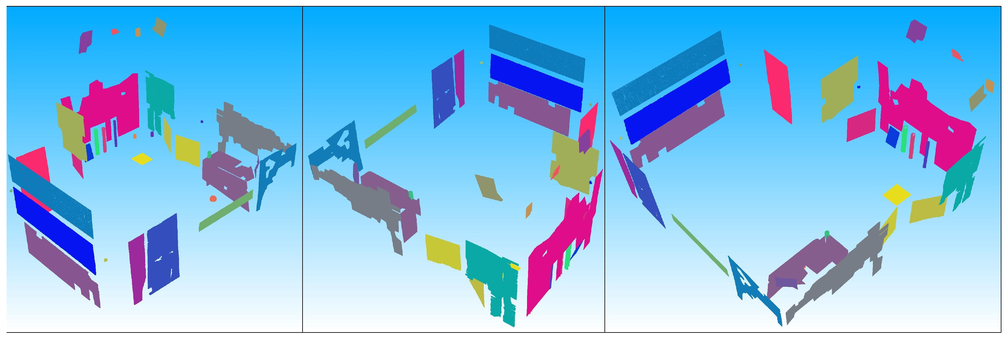
Figure 3. Acquired point clouds of the reference sensor from different views. Each object was separately captured.
Remotesensing 15 02349 g003
Figure 4. (a) TLS viewpoints inside the HiTec laboratory. (b) Three-Dimensional translation uncertainty for each TLS scan.
Remotesensing 15 02349 g004
Subsequently, the TLS point clouds were transformed into the coordinate system of the laser tracker. The transformation is performed using the software Scantra [28], which requires using the centre points of both the TLS targets and corner cube reflectors as inputs to accurately align the point clouds. Figure 4b shows the 3D uncertainty of the translation parameters given using Scantra, which is an average of 0.3 mm. Because all 49 scans are assessed together in the later analysis, the impact of the uncertainties of the transformation parameters on the whole data set can be considered as random. The uncertainties of the transformation parameters can have a positive effect in terms of data augmentation, counteracting overfitting.

2.4. Comparison of TLS and Reference Point Clouds

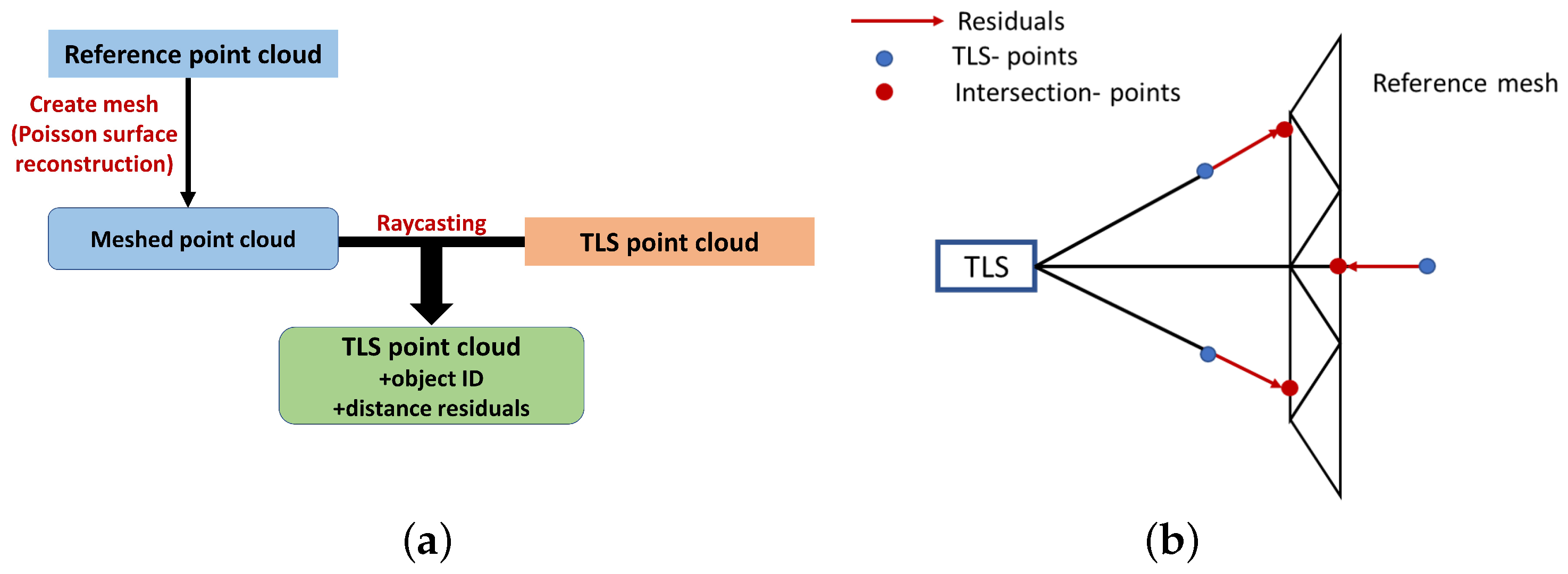
Because we are interested in backward modelling the uncertainties of the TLS point clouds, a comparison between the TLS point cloud and reference point cloud must be performed to calculate the residuals, which will later be our dependent variable y. The procedure to calculate the residuals is illustrated in Figure 5 and outlined as follows:
  • Meshing of the point cloud.
    A mesh is created from the reference point cloud using Poisson surface reconstruction [29]. This approach is preferred over other methods, such as ball pivoting, alpha shapes, and marching cubes, because it produces better results for closed geometries and ensures the topological correctness. Additionally, Poisson surface reconstruction is more robust to sensor noise compared to other methods [30]. As a result, the noise is effectively filtered out and a smooth surface is generated, which accurately represents the geometry. Furthermore, the high point density of the reference point cloud, obtained through multiple measurements, further improves the accuracy of the reconstructed geometry.
  • Raycasting. Raycasting is used to determine the intersection point with the reference mesh for each TLS point, which is achieved by employing the Open3D library in Python [31] (Figure 5b).
    1.
    If an intersection exists, calculate the distance between the intersection point and TLS sensor d i n t e r s e c t , as well as the distance between the TLS sensor and TLS point d T L S .
    2.
    Calculate the distance residuals as = : d T L S d i n t e r s e c t .
    3.
    Save the following information: (1) the object ID, indicating to which object the TLS point belongs, and (2) the distance residuals.
For each TLS point that intersects with the reference mesh, we obtain a difference in the distance, which can be interpreted as a deviation in the distance measurement, along with an object ID that allows us to assign the point to a unique object. Positive distance residuals indicate that the distance measurement was too long, whereas negative distance residuals indicate that the distance measurement was too short.

2.5. Feature Engineering

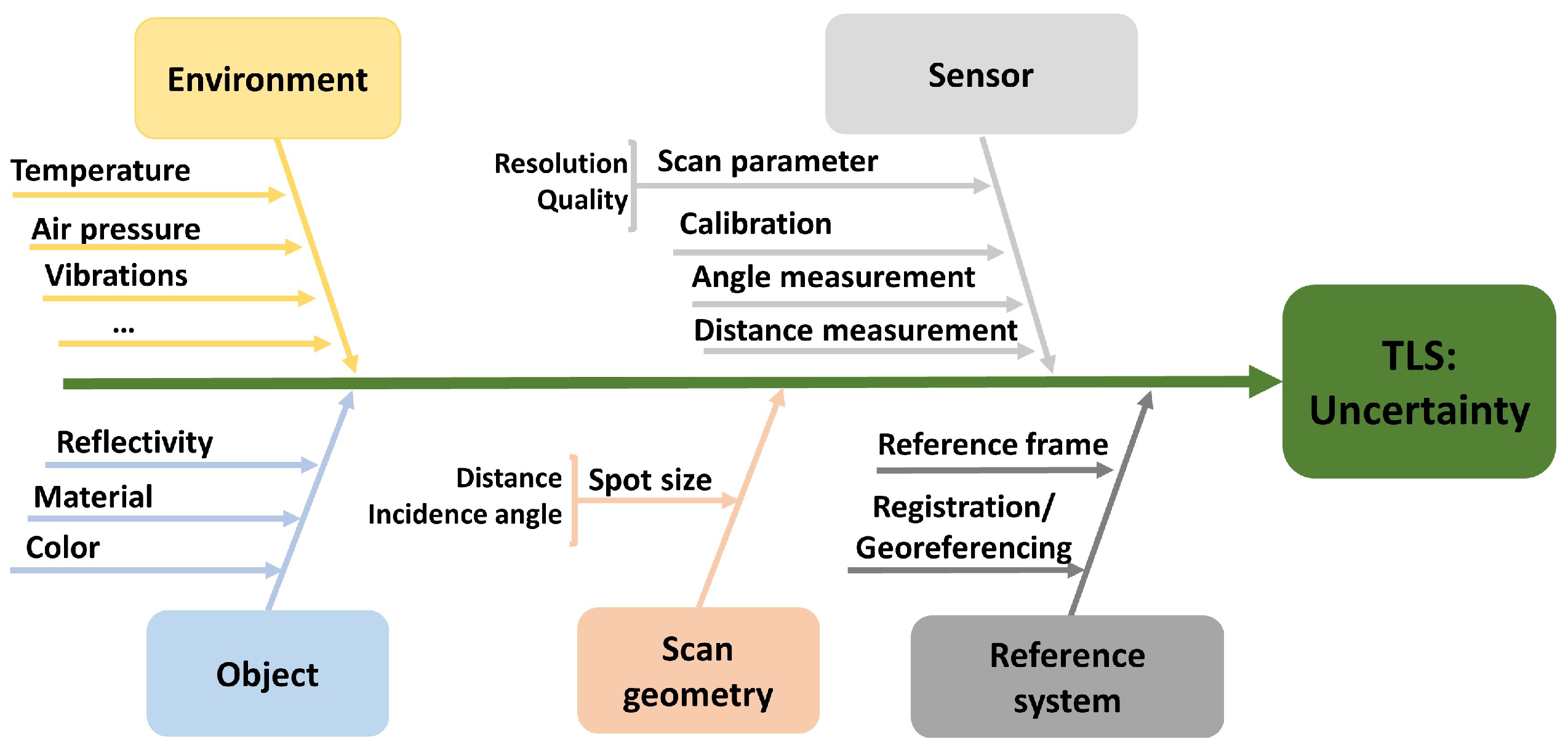
There are numerous factors that influence the uncertainty of a static TLS. Therefore, we calculated different features for each point to assess their contributions to the uncertainties in the distance measurement. These features will be used as the independent variable x i in the uncertainty modelling using various ML regressions approaches. In accordance with the uncertainty budget of TLSs in Figure 6, we focus on features that describe the scan geometry as well as the object because we operated in a controlled environment (stable atmospheric conditions). The following five features are calculated for the TLS points:
  • Intensity: The intensity of the reflected laser beam provides information about the reflectivity of the object and the scan geometry (distance and angle of impact). The raw intensity values can range from 0 to 5 mio. increments for the Z+F Imager 5016. For the regression, the raw intensity values are scaled between 0 and 1 using the formula:
    I = I r a w 5,000,000 [ I n c ]
  • Distance: As the distance increases, the spot size increases, affecting the distance measurement. Distance calculations are performed between TLS points and TLS viewpoint.
    d = ( x t l s x v i e w ) 2 + ( y t l s y v i e w ) 2 + ( z t l s z v i e w ) 2
  • Angle of impact ( α ): The angle between the direction vector from the sensor to the point D P and the point’s surface affects the spot size and distance measurement [12]. The angle of impact α i is calculated in Equation (3) using the point’s normal vector N and is determined through principle component analysis:
    α i = a r c s i n D P i · N i | | D P i | | 2 · | | N i | | 2
  • Spot size (major axis): Depending on the angle of impact, the emitted round laser spot deforms into an ellipse. The spot size’s major axis of the ellipse m a depends on the divergence angle γ , the spot size at the beginning d 0 , and the distance d [32]. It can be calculated using the following formula:
    m a = d 0 + 2 · d · sin ( 2 γ ) cos ( 2 α ) + cos ( 2 γ )
  • Curvature: The curvature provides information about the object’s shape and is calculated from the eigenvalues resulting from the principal component analysis of the k-nearest neighbourhood of a point [33]. With λ 0 λ 1 λ 2 and k = 50 , the curvature can be calculated as follows:
    c u r v = λ 0 λ 0 + λ 1 + λ 2

3. Uncertainty Modelling

The objects analysed in this study differ in their form and material. In the following section, we conduct uncertainty modelling for two heating systems (see Figure 1). A total of 60 million data points are available from backward modelling (see Section 2). Table 2 presents the statistics for the dependent and independent variables. We note that the intensity and the angle of impact cover the entire range of values and that the data set only includes short distances (with a maximum distance of 8.29 m). There is little variation in curvature, which can be attributed to the flatness of the objects.

3.1. Data Analysis

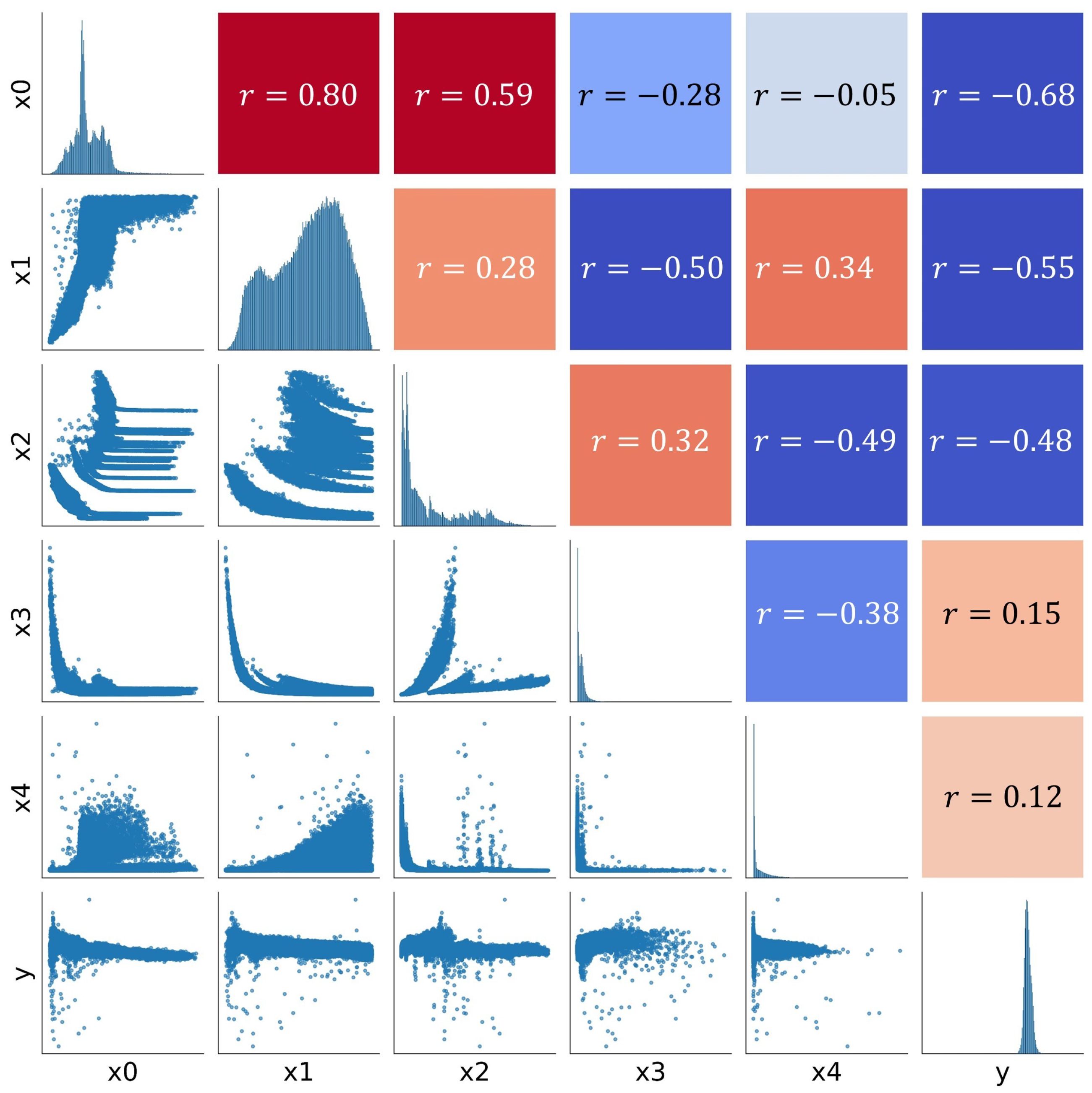
Figure 7 depicts the correlations among the calculated features, revealing that the independent variables are interrelated. Notably, the intensity x 0 is highly positively correlated with the angle of impact x 1 , indicating that the intensity increases with greater angles of impact. This is justified by the radar equation as the laser beam hits the object perpendicularly and with a high angle of impact. Additionally, both the angle of impact and the intensity are positively correlated with the distance x 2 , which is not physically explained and may be attributed to the choice of viewpoint and the limited variation in the distance. Spot size x 3 is negatively correlated with the angle of impact and positively correlated with the distance, in accordance with Equation (4). Moreover, curvature x 4 is positively correlated with the angle of impact and negatively correlated with the spot size, suggesting that larger curvature occurs when the laser beam hits the object perpendicularly, resulting in a small spot size.
The correlations of the independent with the dependent variables y (distance residuals) are particularly interesting. Intensity has the highest correlation with the residuals, with a negative correlation indicating that the residuals become larger with decreasing intensity, which means that the distance tends to be measured too long. Moreover, the angle of impact is negatively correlated with the residuals, whereby the residuals become larger as the angle decreases. In this regard, the small positive correlation of the spot size with the residuals is worth mentioning: as the spot size increases (with a smaller angle of impact), the residuals increase. Lastly, a small positive correlation can be found between the curvature and the residuals, meaning that larger residuals are to be expected as the curvature increases.
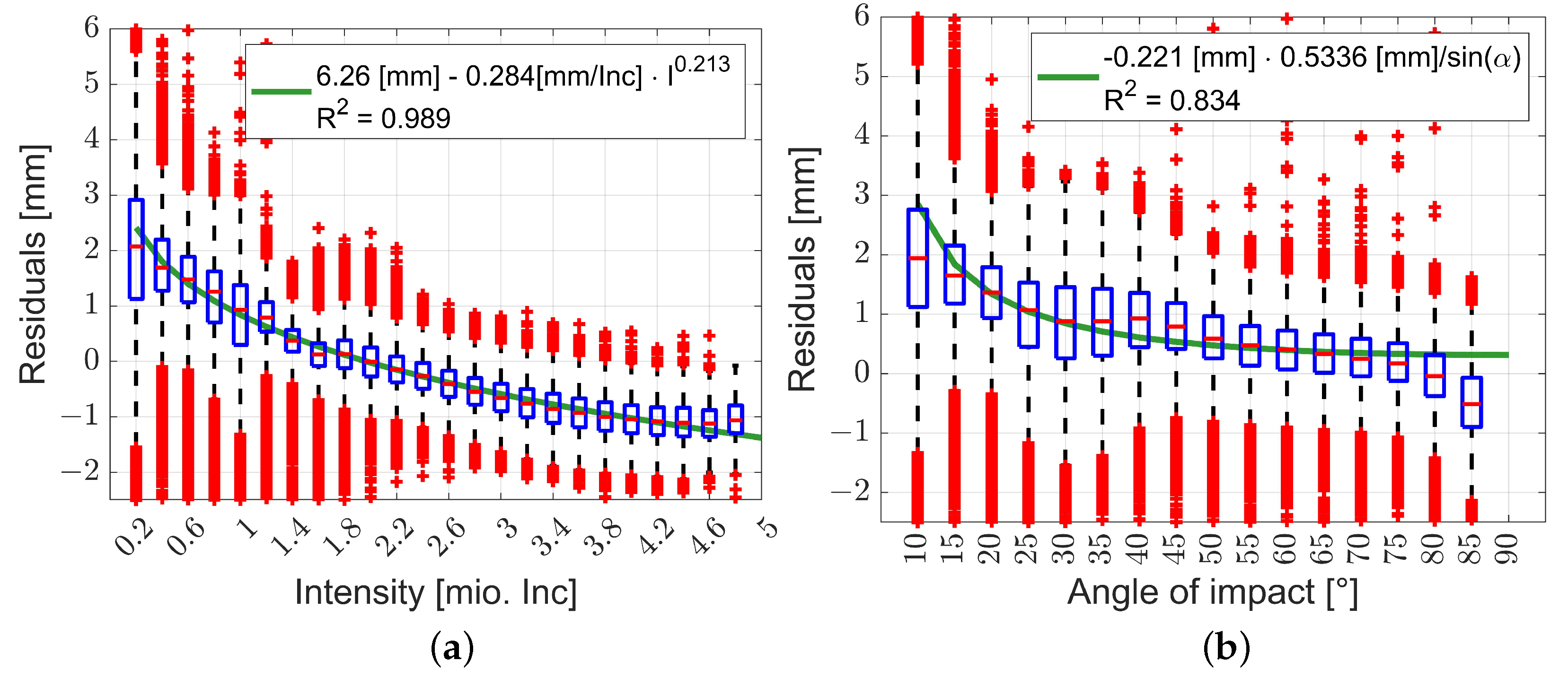
Box plots can help in better understanding the functional relationship between the independent and dependent variables based on the findings of the correlation matrix. Figure 8a shows the course of the distance residuals versus the intensities. It is noticeable that, at low intensities, the distance was systematically measured too long, and at high intensities it was systematically too short. For intensities lower than 1 mio. Inc., the distance was measured too long by more than 1 mm. From intensities of 3.6 mio. Inc., there is a systematic shortening of the distance measurement by 1 mm. When considering only the medians of the distance residuals d r versus the intensity I, their functional relationship follows the same pattern as in the intensity-based model (Equation (6), [15]), with w 0 , w 1 , and b 0 as coefficients.
d r = w 0 · I w 1 + b 0
By fitting a function to the medians of the distance residuals, the green curve in Figure 8a is obtained. To evaluate the quality of fitting, the coefficient of determination from Equation (7) can be used [22]. Here, d r i represents the measured distance residual and d ^ r i represents the predicted distance residuals.
R 2 = Σ ( d r i d ^ r i ) 2 Σ ( d r i d r ¯ ) 2
The coefficient of determination of 0.989 indicates an almost perfect fit and supports the statement that the distance residuals are sufficiently well described using the functional relationship from Equation (6).
Likewise, the distance residuals versus the angle of impact (Figure 8b) show a nonlinear relationship. As the angle of impact α becomes shallower, the distance is measured too long. With a shallow angle of impact of 10°, the distance is measured, on average, 2 mm too long. This relationship can be expressed using the geometrical relationship between the angle of impact and the distance residuals (Equation (8), [23]), with w 0 and b 0 as coefficients. The coefficient of determination of R 2 = 0.834 provides a satisfactory result.
d r = w 0 s i n ( α ) + b 0
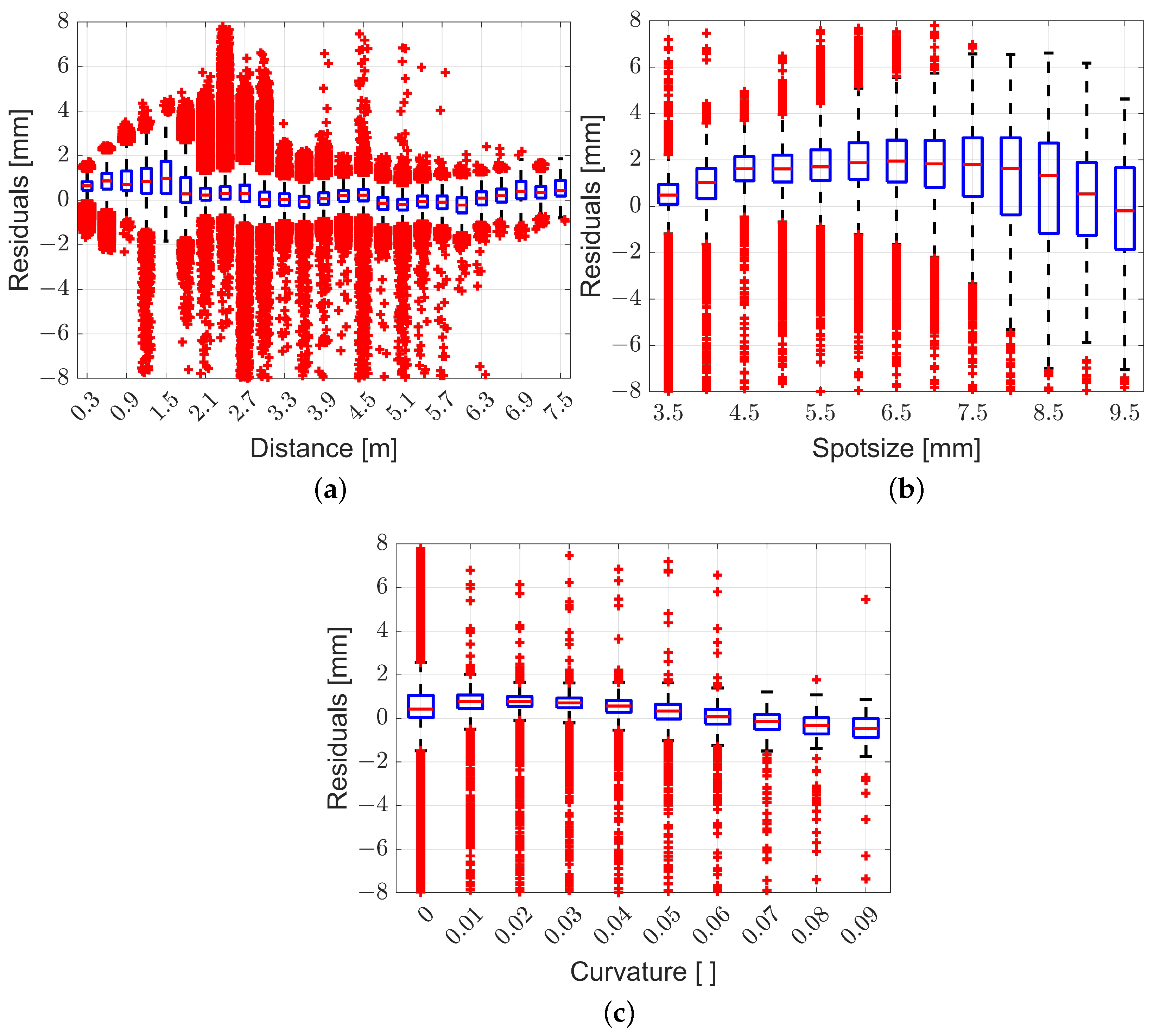
The box plots of the residuals versus the distance in Figure 9a show no clear relationship; nevertheless, it can be observed that the residuals fluctuate around 0.0 mm. In addition, dispersion is larger for short distances. In contrast, a trend can be observed in the box plots of the residuals versus the spot size (Figure 9b). From 3.5 mm to 7.5 mm, the residuals increase and are positive. Subsequently, the residuals decrease with an increasing spot size and reach nearly 0.0 mm at a spot size of 9.5 mm. From the box plot of the residuals versus curvature (Figure 9c), it can be concluded that these features alone do not have a large influence on the distance measurement. However, a linear trend can be observed for the curvature: as the curvature increases, the residuals linearly decrease, which contrasts with the correlation given in Figure 7.

3.2. Regression

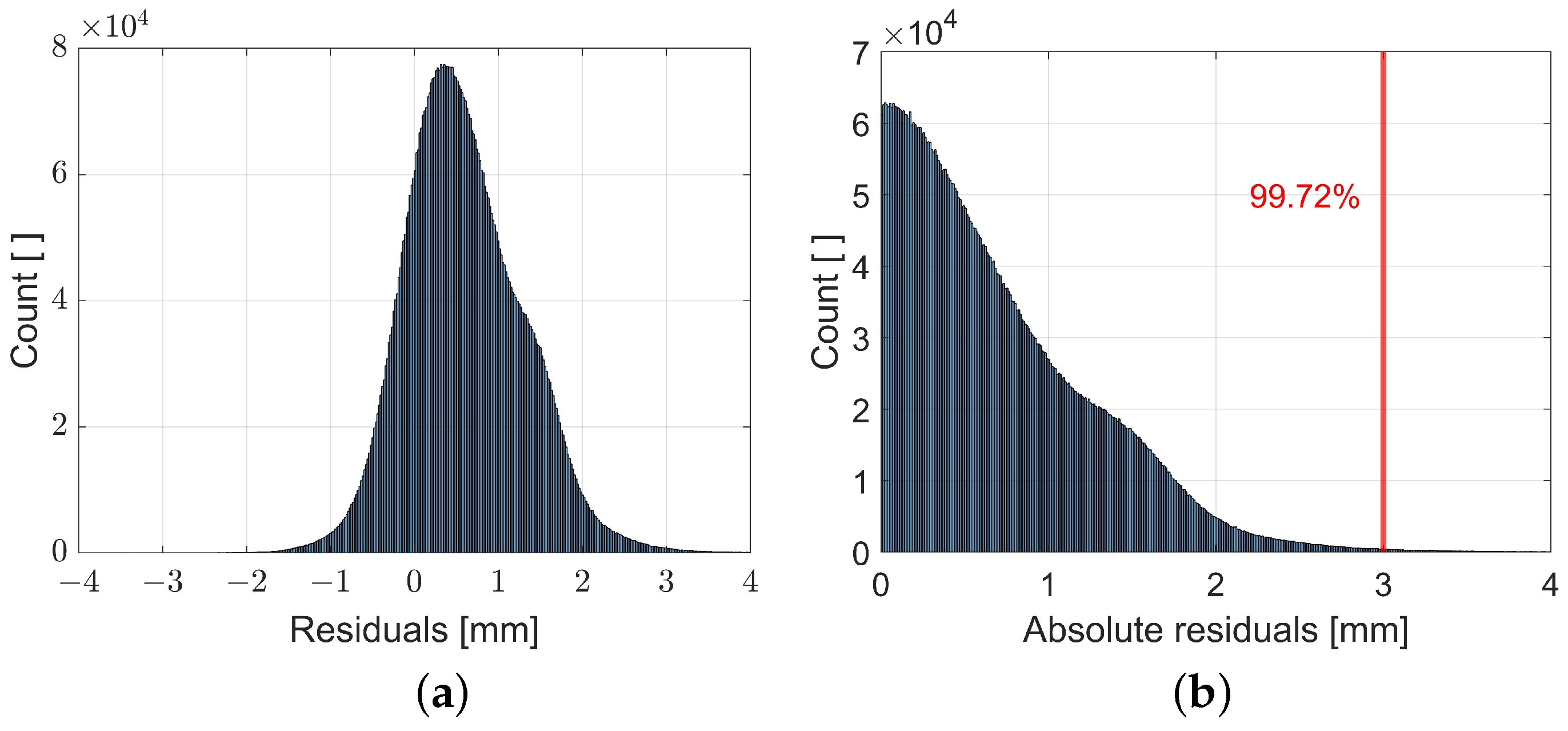
The box plots of the residuals plotted against the independent variables (Figure 8 and Figure 9) reveal a considerable degree of dispersion (blue boxes). In addition, the red crosses indicate that outliers are present in the data set. To obtain reliable regression results, it is necessary to remove these outliers. Figure 10a shows the histogram of the residuals. It can be noted that the residuals are almost normally distributed, although there are some systematic deviations. To remove possible outliers in the data set, we decided to remove all absolute residuals above 3 mm according to the three sigma rule, as they represent 0.3% of the data. The resulting adjusted data were then used for three different types of regression analysis. We did not consider the correlations among the independent variables, as this is beyond the scope of this paper.

3.3. Multiple Linear Regression

The linear relationship between the dependent variable y and the coefficients β can be represented in matrix notation as follows [34]:
y 1 y n b 0 w 1 w 5 f w , b 0 ( x ) = 1 x 1 , 0 x 1 , 4 1 x n , 0 x n , 4 b 0 w 1 w 5 X · b 0 w 1 w 5 β + ϵ 1 ϵ n b 0 w 1 w 5 ϵ
Using the ordinary least-squares approach (minimizing the square root of the residuals), the unknown regression coefficients can be estimated with the following:
β ^ = ( X T · X ) 1 · X T · y

3.4. Multiple Nonlinear Regression

If we take into account the nonlinear relationships for the intensity and the angle of impact from Section 3, we can establish the following multiple nonlinear relationship:
f w , b 0 ( x ) = b 0 + w 1 x i , 0 w 2 + w 3 s i n ( x i , 1 ) + w 4 x i , 2 + w 5 x i , 3 + w 6 x i , 4 + ϵ
The unknown regression coefficients are iteratively determined using nonlinear least-squares method by minimizing the square root of the residuals. For this linearization of Equation (11), using Taylor series expansion is required. In this process, approximate values for the coefficents β 0 and w i are introduced.
Δ β ^ = ( A T · A ) 1 · A T · δ y
with :
A = f w , b 0 ( x ) 1 b 0 f w , b 0 ( x ) 1 w 1 f w , b 0 ( x ) 1 w n f w , b 0 ( x ) n b 0 f w , b 0 ( x ) n w 1 f w , b 0 ( x ) n w n

3.5. XGBoost Regressor

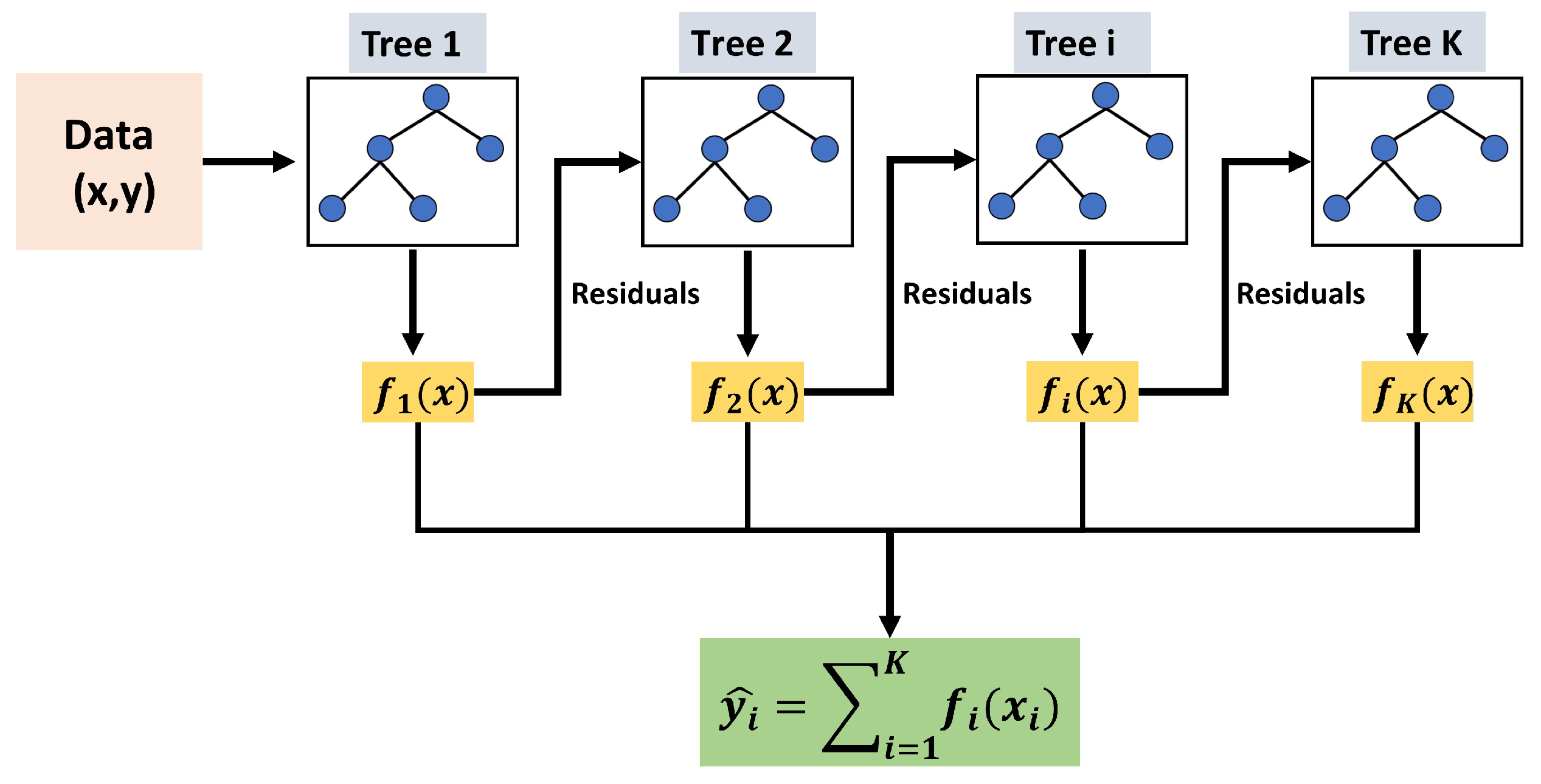
XGBoost, developed by [35], stands for “eXtreme Gradient Boosting”, which is typically used for classification and regression tasks. The basis of the approach are classification and regression trees (CARTs). The general process is outlined in Figure 11. The approach is based on ensemble decision trees, wherein each tree learns from the residuals of the previous tree. The final prediction y ^ i is obtained from the sum of all trained CARTs:
y ^ i = Σ k = 1 K f k ( x i ) , f k F
where K represents the number of trees, f k ( x i ) as the result from one tree, and F denotes the set of all possible CARTs. The objective of the model consists of one loss function L ( θ ) and one penalty term Ω ( θ ) to address the complexity of the model. It uses Σ i = 1 n l y i , y ^ i ( t ) to calculate the difference between the predicted value and the actual value of the loss function. The term ω ( f ) defines the complexity of the tree, with T as the number of leaves, ω as scores on leaves, γ to describe the leaf penalty coefficient, and λ to ensure that the leaf scores do not become too large.
L ( θ ) = Σ i = 1 n l y i , y ^ i ( t )
Ω ( θ ) = Σ i = 1 t ω ( f i )
ω ( f ) = γ T + 1 2 λ j = 1 T ω j 2
O b j = L ( θ ) + Ω ( θ )
The processing of the model is additive, as the t-th prediction y ^ i ( t ) is the sum of the prediction of the new tree f t ( x i ) and the prediction of the previous iteration y ^ i ( t 1 ) .
y ^ i ( t ) = y ^ i ( t 1 ) + f t ( x i )
The updated objective from Equations (19) and (20) is given as:
O b j = Σ i = 1 n l y i , y ^ i ( t 1 ) + f t ( x i ) + Ω ( θ )
Using the second-order Taylor expansion of the loss function, the objective can be approximated as in Equation (22), where g i and h i represent the first- and second-order derivatives, respectively.
O b j = Σ i = 1 n l y i , y ^ i ( t 1 ) + g i f t ( x i ) + 1 2 h i f t 2 ( x i ) + Ω ( θ )
g i = y ^ i t 1 l y i , y ^ i ( t 1 )
h i = 2 y ^ i t 1 l y i , y ^ i ( t 1 )
During the construction of the individual trees, a gain parameter G a i n is calculated to decide if a leaf should be divided into several leaves, as follows:
G a i n = 1 2 G L 2 H L + λ + G R 2 H R + λ + ( G L + G R ) 2 H L + H R + λ γ
G = Σ i I g i
H = Σ i I h i
Here, G L and H L represent the results for the left leaves, G R and H R represent the results for the right leaves, and λ is a regularization parameter. Additionally, the parameter γ prunes the tree, and as soon as the gain is smaller than γ , the leaf is not subdivided.

Hyperparameter

In XGBoost, achieving high model performance requires an important process called hyperparameter tuning. This involves modifying the parameter values of a model to manage its complexity, regularization, and learning rate, ultimately enhancing its capability to generalize and perform well with new data. In the following section, we will describe and discuss approaches to tune the hyperparameter as well as the primary parameters used in XGBoost and their impact on model performance [36].
The hyperparameters play a crucial role in determining the performance of the XGBoost model. Several methods are available to obtain the optimal hyperparameters (refer to Figure 12). In the optimization process, the hyperparameters are selected to minimize the defined loss function. Grid searches evaluate all possible combinations of hyperparameters to determine their suitability, and the combination with the smallest loss is selected as the optimal choice. Random searches select hyperparameters at random, and after certain combinations have been tested, the combination with the smallest loss is selected. In contrast, the Bayesian optimizer chooses the most likely combination of hyperparameters that minimizes the loss function. It leverages the results of previously evaluated combinations, leading to faster hyperparameter tuning. Due to its efficiency, the Bayesian optimizer was utilized for hyperparameter tuning in this work. Specifically, we used the hyperopt [37] Python library for this purpose. During hyperparemeter tuning, the models were trained using the training data set, and the RMSE of the validation data set was minimized (see Section 3.6).
XGBoost has a number of hyperparameters that influence training and can lead to overfitting (model too complex, small regularization) or underfitting (model too simple, large regularization). The following hyperparameters were tuned during the Bayesian optimization using the specified search spaces.
  • Max_depth: The max_depth parameter determines the depth limit of the trees within a model. Increasing the max_depth value creates more intricate models. Search space = [2–8].
  • N_estimators: The number of trees within a model is controlled by the n_estimators parameter. Raising this value generally enhances the performance of the model, but it can also increase the risk of overfitting. Search space = [20–150].
  • eta: The learning rate governs the size of the optimizer’s steps when updating weights in the model. A smaller eta value results in more precise but slower updates, whereas a larger eta value leads to quicker but less precise updates. Search space = [0–1].
  • reg_lambda: The lambda parameter, also known as the L2 regularization term on weights, regulates the weight values in the model by adding a penalty term to the loss function. Search space = [0–20].
  • alpha: The alpha parameter is responsible for the L1 regularization term on the weight values of the model by adding a penalty term to the loss function. Search space = [0–20].
  • subsample: The subsample parameter determines the proportion of observations used for each tree in the model. Search space = [0–1].
  • colsample_by_tree: The colsample_by_tree parameter regulates the fraction of features used for constructing each tree in the model. Setting a lower colsample_by_tree value results in smaller and less intricate models that can assist in avoiding overfitting. Search space = [0–1].
  • min_child_weight: The min_child_weight parameter specifies the minimum sum of instance weights needed in a node before the node will be split. Setting a larger min_child_weight value results in a more conservative tree as it requires more samples to consider splitting a node. Search space = [0–20].

3.6. Training of the Models Using Cross Validation

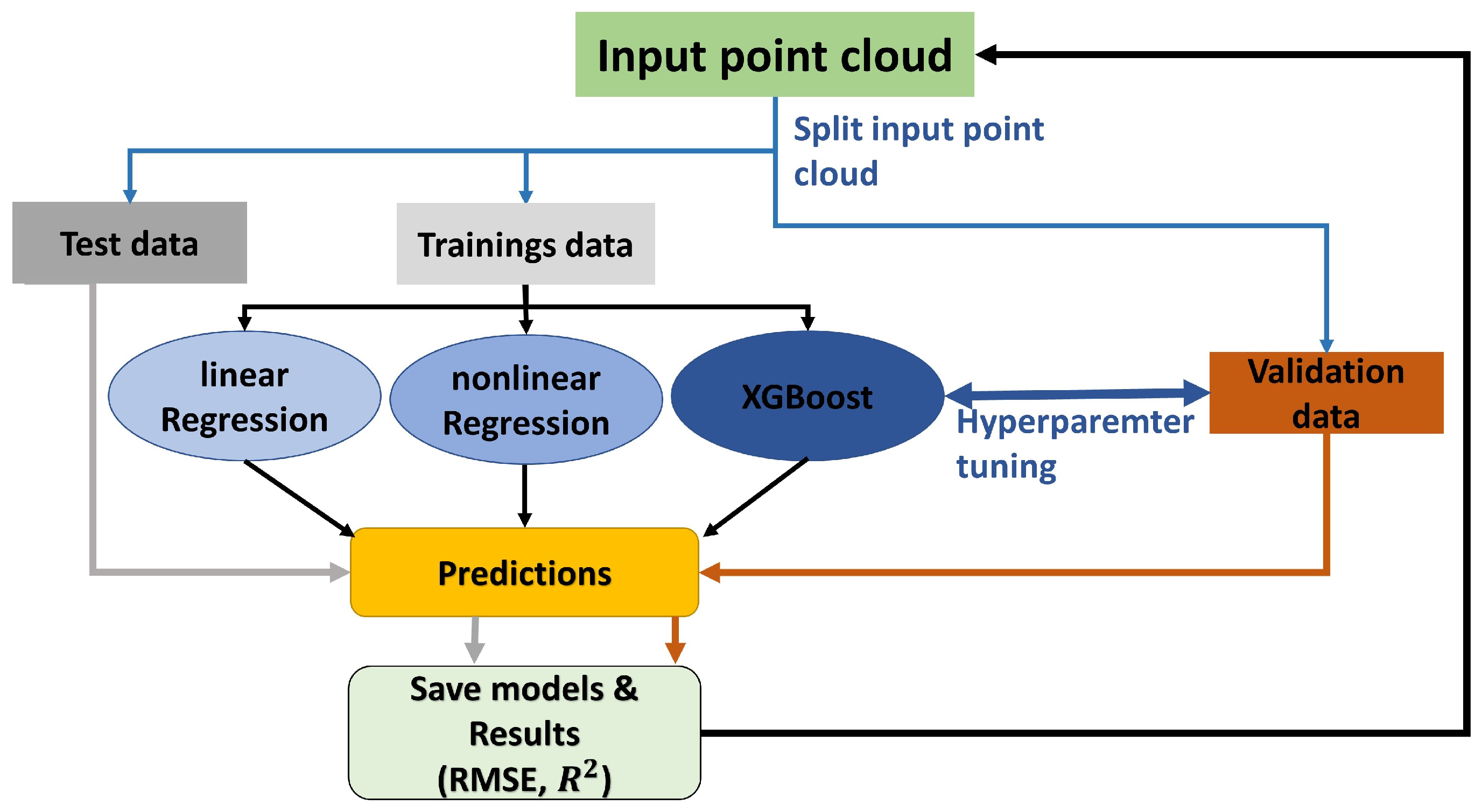
The three ML models utilized in this study were all trained and validated using the same procedure, as depicted in Figure 13. The validation process is similar to the k-fold cross validation. First, the input point cloud was divided into three distinct data sets:
  • Input point cloud: This consisted of 49 TLS scans from two different objects (two heating systems), resulting in 98 independent objects.
  • Validation data (1): A validation data set was created by randomly selecting objects from the 98 scanned objects until its size was greater than 20% of the entire input point cloud. The validation data set was independent from the training data set as no temporal correlation was present.
  • Training data (2) and Test data (3): The remaining point cloud was randomly split into training (80%) and test (20%) data. The test data set was not independent from the training data set as correlations existed due to data from the same scans.
All three models were trained using the training data set, and their performance was evaluated and compared using the coefficient of determination (Equation (7)) and the RMSE (Equation (28)) for both the test and validation data sets. The calculated values were stored for each iteration. The entire process was repeated 120 times (similar to sampling with replacement).
R M S E = 1 n ( d r i d ^ r i ) 2
It is worth noting that the validation data played a crucial role in training the XGBoost regressor (refer to Figure 13). During Bayesian hyperparameter tuning (hyperopt [37]), the XGBoost models were trained with the training data set and aimed to minimize the loss function (Equation (28)) for the validation data set.

4. Analysis of Regression Results

The analysis of the regression results is divided into two parts. First, we examine the individual regression models to determine the effects of the independent variables and the resulting coefficients. Secondly, we assess the quality measures, including the coefficient of determination and RMSE, to evaluate the quality of the model prediction.

4.1. Feature Importance

To begin evaluating the quality of the regressions, it is important to understand how each independent variable affects the three models. A useful approach for this purpose is to investigate the partial dependencies of the independent variable with respect to the dependent variable. The partial dependencies can be determined using the following equation:
f ¯ S ( X S ) = 1 N Σ i = 1 N f ( X S , x i C )
where x i C represents the values occurring in the training data and X S represents the independent variables for which we want to calculate the partial dependencies [22].
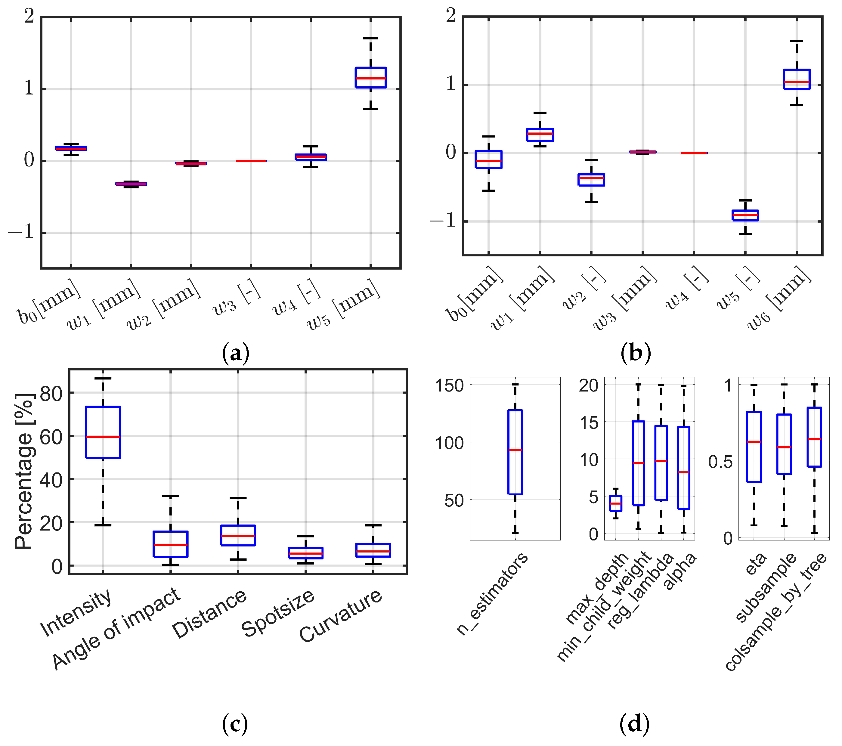
Figure 14 displays the partial dependencies of the independent variable on the dependent variable for each regressor trained on the entire input point cloud. The multiple linear regression model (blue) shows that the dependency of the distance residuals decreases linearly with increasing intensity, angle of impact, and distance, whereas the dependency increases linearly with curvature. Furthermore, it is observed that the dependency remains constant with respect to the spot size, indicating that the influence of spot size can be neglected. In contrast, nonlinear trends are observed for the multiple nonlinear regression (red line). For intensity and angle of impact, the form of the curve aligns with those from Section 3.1. Additionally, it can be noted that the dependency decreases with increasing spot size. The partial dependencies of the XGBoost regressor (green line) are particularly interesting because this model can be considered to be a “black box”. Notably, the partial dependency follows a step-like behaviour, which results from the tree-based method. Regarding intensity, the same behaviour can be observed as in the other two models: intensity has the largest partial dependency, and the dependency decreases with increasing intensity. In this case, the decrease is almost linear. Moreover, it can be seen that the angle of impact, spot size, and curvature do not vary much, and thus do not have as strong an influence as intensity.
The distribution of the coefficients of the linear and nonlinear models, shown in Figure 15a,b, reveals that some coefficients display larger fluctuations than others. Specifically, the linear model shows that the curvature ( w 5 ) has the highest variation, whereas the distance ( w 3 ) has the lowest. The offset ( b 0 ) is positive, and the weights w 1 and w 2 assigned to the intensity and angle of impact are negative. This implies that the residuals decrease with increasing intensity and angle of impact. In the nonlinear model, the offset ( b 0 ) is negative, and the variation is highest for the curvature ( w 6 ) and lowest for the distance ( w 4 ). The XGBoost regressor, which is considered to be a “black box”, does not provide weights for the independent variables. However, its implemented algorithm offers the possibility to calculate the feature importance, which sheds light on the model’s behaviour. Figure 15c shows the feature importance calculation as box plots from 120 samplings, conforming the conclusions from Figure 14. The intensity had the most significant influence with a median of 60%, followed by the distance with 13%. The angle of impact still had a noticeable influence with 9%, whereas the spot size and the curvature had medians of almost 5% and 6%, respectively. The hyperparameters of the XGBoost regressor presented in Figure 15d were estimated with Bayesian hyperparameter tuning using the validation data set. The figure reveals that all hyperparameters showed larger variations, except for the maximum depth of the tree. The 25% and 75% quantiles of the distribution were two and five, respectively, which corresponds with the number of independent variables (intensity, angle of impact, distance, spot size, and curvature) used for training. In summary, a conclusion of possible hyperparameters for later models can be drawn from this figure. The medians of the respective hyperparameters are useful if the entire data set is to be trained with one XGBoost model.

Quality of the Regression

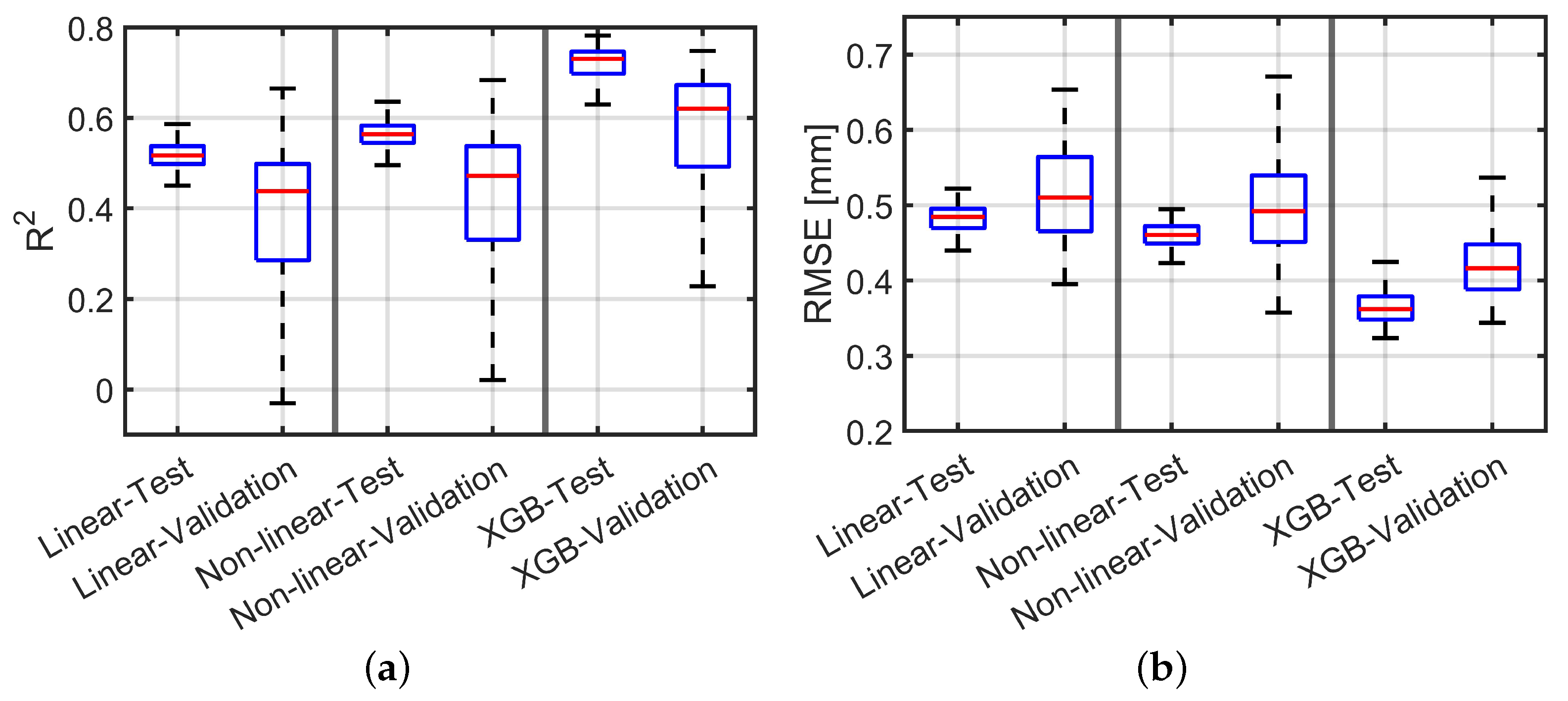
To compare the regression results of the 120 runs for the three models, we considered the coefficient of determination and RMSE as quality measures. Both measures are presented in Figure 16 in the form of box plots for the test and validation data sets. Regarding the quality measures, it is evident that all three models deliver satisfactory results as the RMSE is smaller than 0.5 mm. However, all methods achieved better results for the test data set compared to the validation data set, indicating overfitting of the training data set in some runs. The dispersion (blue boxes) of the quality measures was also larger for all methods for the validation data set.
Specifically, the multiple linear regression achieved the smallest coefficient of determination, with a median value of 0.52 for the test data set and a mean value of around 0.44 for the validation data set. On the other hand, the multiple nonlinear regressions performed slightly better than the linear regressions, achieving coefficients of determination of 0.56 and 0.47 for the test and validation data sets, respectively. Furthermore, the dispersion (blue box) of the coefficient of determination for the validation data set decreased compared to multiple linear regression. The XGBoost regressor achieved the best results for both the test and the validation data sets, with coefficients of determination of 0.73 and 0.62 , respectively, which represents an improvement of 30% compared to the multiple nonlinear regression. The same behaviour was observed with regard to the RMSE. The multiple linear regression delivered satisfactory results for both the test and the validation data sets, with a mean RMSE of 0.49 mm and 0.51 mm, respectively. The multiple nonlinear regressions achieved slightly improved results compared to the linear regression, with an RMSE of 0.46 mm for the test data set and 0.49 mm for the validation data set. The XGBoost regressor achieved the best results for both data sets, with an RMSE of 0.36 mm for the test data set and 0.42 mm for the validation data set, resulting in an improvement of 20% and 10% compared to multiple nonlinear regression.

4.2. Distance Calibration Using XGBoost Regressor

As shown in the previous section, the deviations in the distance measurement can be modelled as a function of five influences using three ML regressions. Among these, the XGBoost regressor offers the best results in term of the coefficient of determination and RMSE. Given that the distance deviations are systematic, it is possible to calibrate the TLS distance measurement using the XGboost regression results. The calibration procedure involves calculating features such as intensity, angle of impact, distance, spot size, and curvature, followed by predicting distance residuals using 120 XGBoost regressors. The average of the 120 predictions is then calculated as the final distance residual. The TLS distance measurement d m e a s is then calibrated by subtracting the predicted distance residuals d ^ r from d m e a s , as shown in Equation (30).
d c a l = d m e a s d ^ r
To reduce variance, all 120 XGBoost models were used to predict the systematic deviations in the distance measurement. Averaging the 120 XGBoost models (bagging) leads to a more accurate prediction. Figure 17 illustrates the results of calbrating the distance measurement for the entire heating data set using the average prediction of the 120 XGBoost regressors. The distribution of the residuals of the raw and calibrated point clouds indicates that the calibration results in a normal distribution. During the calibration, the mean of the distribution of the distance residuals decreased from 0.5 mm to 0.02 mm, corresponding to a 96 % reduction. Additionally, the standard deviation decreased from 0.69 mm to 0.36 mm, a reduction of 48 % . Figure 17b shows that the prediction aligns well with the actual residuals, following a linear trend. However, some larger deviations cannot be predicted with sufficient accuracy, which can be caused by the precision of the TLS.

4.3. Real Case Application

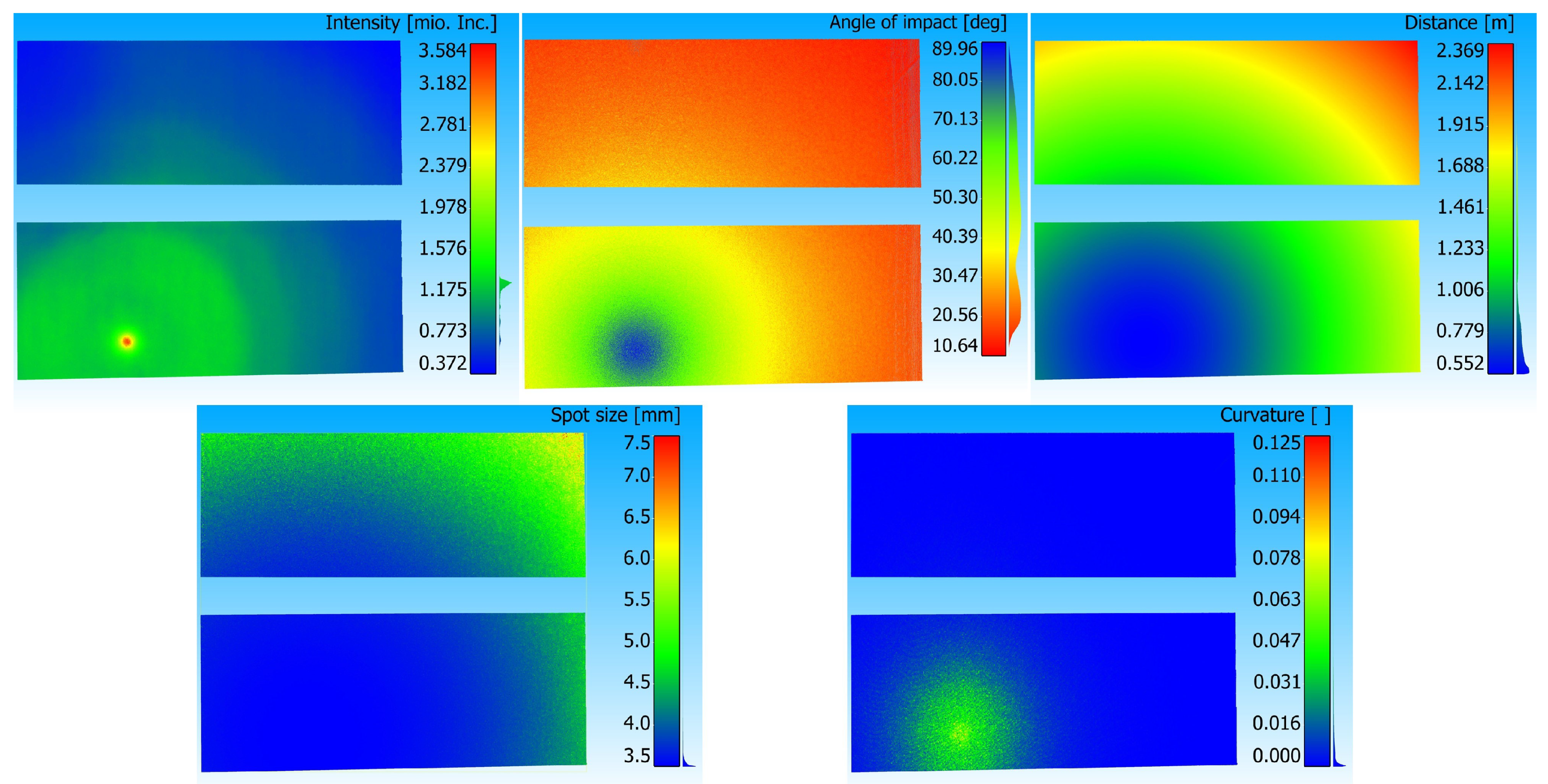
For further validation, a scan was taken in the HiTec lab that was not included in the training and validation data sets and was, therefore, completely independent of the XGBoost model training. All necessary features were calculated for the point cloud, and these can be found in Figure 18. Based on the distance and the angle of impact, it is apparent that the viewpoint is directly in front of the two heating systems.
On the ond hand, Figure 19 shows the real residuals of the reference mesh and the predicted residuals of the XGBoost regressors. On the other hand, the residuals resulting from the calibration of the distance measurement are displayed. It is well visible that the distance was measured too short (blue) at the point where the laser beam hits perpendicular, and high intensities were reflected back, whereas in other areas with shallower angles of impact and lower intensities, the distance was measured too long (red).
Regarding the averaged prediction from 120 models, it can be observed that the effects mentioned earlier were modelled. The prediction reveals that at high intensities and a with perpendicular angle of impact, the distance measured was predicted to be too short, whereas for the remaining area of the point cloud, the distance measured was predicted to be too long. The circular behaviour of the distance residuals around the area where the laser beam hits perpendicularly was also modelled. Looking at the residuals with the calibrated distance measurement, it is evident that the distance is generally measured too short instead of too long. The histograms in Figure 20 show that the calibration caused the mean value of the residuals to shift from 0.97 mm (raw data) to 0.10 mm (calibration). Additionally, the standard deviation of the residuals decreased from 0.41 mm to 0.36 mm.
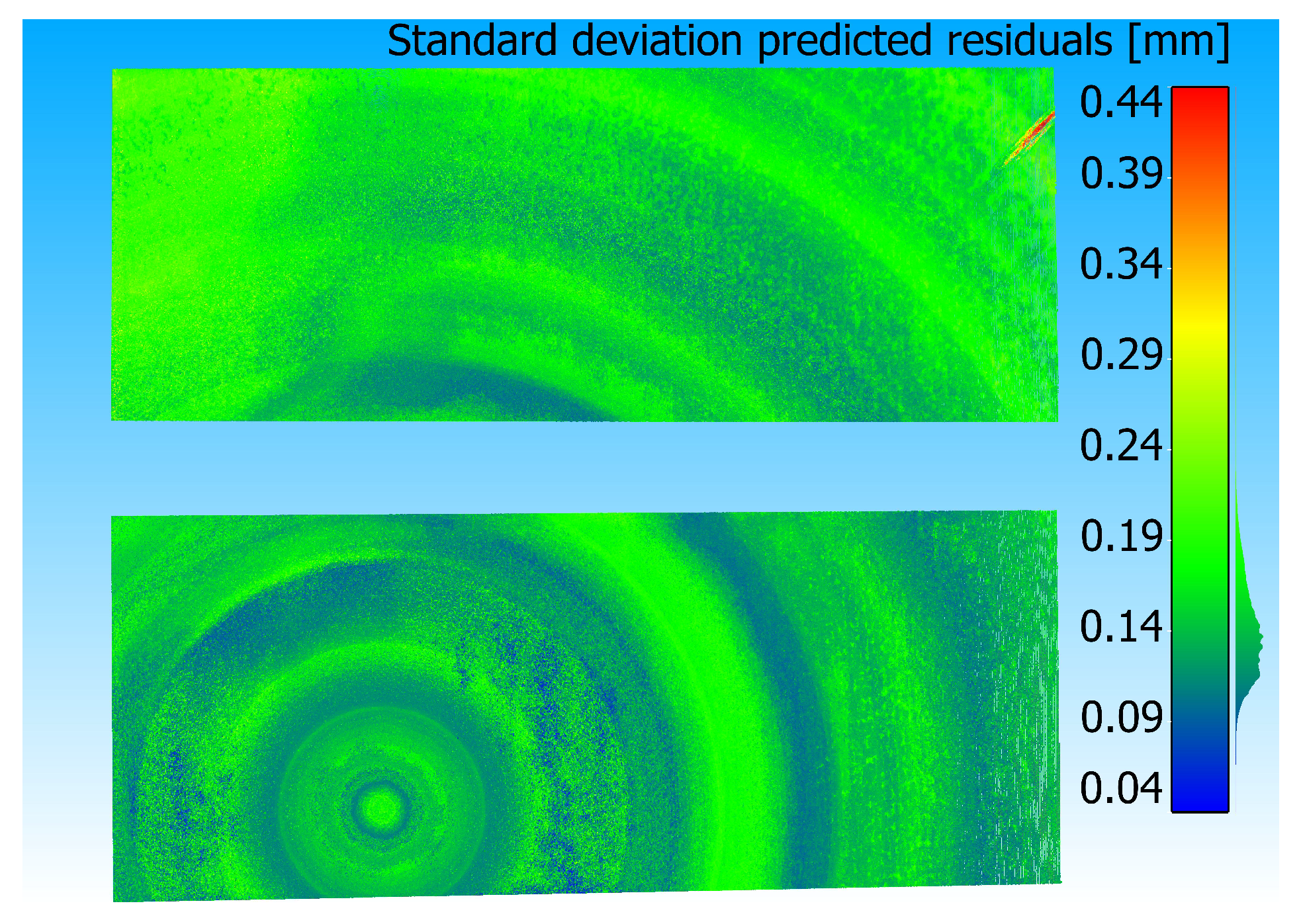
Finally, predicting with 120 models has the advantage of determining the standard deviation of the prediction for each point, providing a separate quality measure (Figure 21). Analysing the standard deviation of the predicted residuals can reveal where the XGBoost regressors are consistent and where there are higher deviations. The standard deviations scattered slightly, with the majority falling in the range of [0.09–0.2 mm]. A circular pattern was also evident in the standard deviations when the angle of impact was 90°. The highest standard deviation, around 0.44 mm, was found at the top right of the top heating (refer to Figure 19). This is the area where the prediction did not match the real residuals at all (real = negative, prediction = positive).

5. Discussion

The results of this work demonstrate a novel method of calibrating TLS distance measurements by using a highly accurate reference point cloud and gradient boosting trees. This approach effectively reduces the systematic effects caused by object properties and scan geometry, resulting in the increased accuracy of the TLS point cloud. The recorded data set and a real case example were used to show that calibration with an ML model can minimize the residuals of the reference point cloud, bringing the mean value of the residuals closer to 0.0 mm and slightly decreasing the standard deviations of the residuals. Compared to the previous approach, which divides the distance deviations into four classes [23], this is a considerable improvement.
Concerning the angle of impact, findings from other publications [13,14] have confirmed that the distance is measured too long when the angle becomes shallower. The proposed ML model incorporates scan geometry information to predict systematic distance deviations accurately. This approach shares similarities with the methodology used in [12], wherein the authors modelled measurement noise as a function of both distance and incidence angle. However, our approach differs in that we focused on effectively correcting distance measurements rather than modelling the noise.
Furthermore, we applied the functional relationship between intensity and distance residuals from the study in [15]. However, unlike their study wherein the precision was modelled, we modelled the systematic deviation in our publication. Our analysis revealed that at high intensities, the distance measurement was measured too short by up to 1 mm. This behaviour could not be taken into account in [15] because only precision could be modelled there. By modelling the systematic deviation, we were able to account for it and improve the accuracy of the distance measurements, especially at high intensities. In contrast to TLS calibration approaches, such as that described in [8], our approach modelled the TLS distance measurement as a function of scanner external influences, including object properties and scan geometry, rather than as a distance offset. Consequently, our calibration method can be used as an additional step in TLS calibration. Moreover, our prediction of distance deviation can have broader applications, such as in viewpoint planning and weighting of points for registration using the iterative closest-point method or deformation analysis.

6. Conclusions

This paper tackled the critical issue of systematic deviations in TLS distance measurements. To achieve this, a comprehensive data set for the Z+F Imager 5016 was recorded using a reference sensor with superior accuracy. This enabled the investigation of the impact of various factors on distance measurements through backward modelling. The analysis revealed that both the intensity and the angle of impact exert the most significant influences, modelled as nonlinear relationships. Accounting for these effects resulted in more precise prediction outcomes compared to multiple linear regression.
Furthermore, this paper introduced an XGBoost approach to predict the distance residuals. The XGBoost regressor proved superior to conventional ML approaches, showing excellent performance in modelling nonlinear relationships, as evidenced by its lower RMSE and higher coefficient of determination. Additionally, a routine was developed that split the data set into validation, test, and training sets, and Bayesian hyperparameter tuning minimized the overfitting effect. Using 120 trained XGBoost regressors, this paper demonstrated a TLS distance deviation prediction, using an independent scan that was not part of the training process. The results showed that the prediction reflects the true residuals accurately, and calibration of the distance measurement leads to enhanced outcomes.
The results of this study demonstrate the potential of ML approaches, particularly the XGBoost regressor, to improve the accuracy of distance measurement in TLSs. While this study focused on a single object produced from one material, future work will explore the applicability of ML approaches to a broader range of objects and materials. This will require careful evaluations of additional features and potential adjustments to the models. In particular, we will investigate the suitability of neural network approaches for predicting systematic deviations in distances. In addition, the correlations between the independent variables will be considered in further investigations. We also plan to extend the data set through additional measurements, with a particular focus on objects that exhibit a wider range of distances.
It is important to investigate whether the distance measurement calibration we proposed is only applicable to the specific sensor used in this study or if it can be transferred to other sensors of the same type or from different manufacturers. Additionally, identifying a suitable calibration routine that can efficiently and accurately perform distance calibrations is crucial. Such an investigation can provide valuable insights into the generalizability of our approach and its potential to improve distance measurement accuracy across different TLS sensors. By expanding the scope of our study in these ways, we aim to build on the promising results presented here and contribute to the ongoing development of more accurate and efficient TLS technologies.

Author Contributions

Conceptualization, J.H. and H.A.; methodology, J.H. and H.A.; software, J.H.; validation, J.H.; formal analysis, J.H. and H.A.; investigation, J.H. and H.A.; resources, J.H. and H.A.; data curation, J.H.; writing—original draft preparation, J.H. and H.A.; writing—review and editing, H.A.; visualization, J.H.; supervision, H.A. All authors have read and agreed to the published version of the manuscript.

Funding

The research presented was carried out within the scope of the collaborative project “Qualitätsgerechte Virtualisierung von zeitvariablen Objekträumen (QViZO)”, which was supported by the German Federal Ministry for Economic Affairs and Energy (BMWi) and the Central Innovation Programme for SMEs (ZIM FuE- Kooperationsprojekt, 16KN086442).

Data Availability Statement

The data presented in this study are available on request from the corresponding author.

Conflicts of Interest

The authors declare no conflict of interest.

Abbreviations

The following abbreviations are used in this manuscript:
TLSterrestrial laser scanner
MLmachine learning
GUMGuide to the Expression of Uncertainty in Measurement
RMSEroot-mean-square error
CART classification and regression trees

References

  1. Joint Committee for Guides in Metrology. Evaluation of Measurement Data—Guide to the Expression of Uncertainty in Measurement. 2008. Available online: https://www.iso.org/sites/JCGM/GUM-JCGM100.htm (accessed on 9 March 2023).
  2. Alkhatib, H.; Neumann, I.; Kutterer, H. Uncertainty modeling of random and systematic errors by means of Monte Carlo and fuzzy techniques. J. Appl. Geod. 2009, 3, 67–79. [Google Scholar] [CrossRef]
  3. Alkhatib, H.; Kutterer, H. Estimation of Measurement Uncertainty of kinematic TLS Observation Process by means of Monte-Carlo Methods. J. Appl. Geod. 2013, 7, 125–134. [Google Scholar] [CrossRef]
  4. Neitzel, F. Untersuchung des Achssystems und des Taumelfehlers terrestrischer Laserscanner mit tachymetrischem Messprinzip. In Terrestrisches Laser-Scanning (TLS 2006), Schriftenreihe des DVW, Band 51; Wißner-Verlag: Augsburg, Germany, 2006; pp. 15–34. [Google Scholar]
  5. Neitzel, F. Gemeinsame Bestimmung von Ziel-, Kippachsenfehler und Exzentrizität der Zielachse am Beispiel des Laserscanners Zoller+ Fröhlich Imager 5003. In Photogrammetrie-Laserscanning-Optische 3D-Messtechnik, Beiträge der Oldenburger 3D-Tage; Herbert Wichmann Verlag: Heidelberg, Germany, 2006; pp. 174–183. [Google Scholar]
  6. Holst, C.; Kuhlmann, H. Challenges and present fields of action at laser scanner based deformation analyses. J. Appl. Geod. 2016, 2016, 17–25. [Google Scholar] [CrossRef]
  7. Medić, T.; Holst, C.; Janßen, J.; Kuhlmann, H. Empirical stochastic model of detected target centroids: Influence on registration and calibration of terrestrial laser scanners. J. Appl. Geod. 2019, 13, 179–197. [Google Scholar] [CrossRef]
  8. Medić, T.; Holst, C.; Kuhlmann, H. Optimizing the Target-based Calibration Procedure of Terrestrial Laser Scanners. In Allgemeine Vermessungs-Nachrichten: AVN; Zeitschrift für alle Bereiche der Geodäsie und Geoinformation; VDE Verlag: Berlin, Germany, 2020; pp. 27–36. [Google Scholar]
  9. Muralikrishnan, B.; Ferrucci, M.; Sawyer, D.; Gerner, G.; Lee, V.; Blackburn, C.; Phillips, S.; Petrov, P.; Yakovlev, Y.; Astrelin, A.; et al. Volumetric performance evaluation of a laser scanner based on geometric error model. Precis. Eng.-J. Int. Soc. Precis. Eng. Nanotechnol. 2015, 40, 139–150. [Google Scholar] [CrossRef]
  10. Gordon, B. Zur Bestimmung von Messunsicherheiten Terrestrischer Laserscanner. Ph.D. Thesis, Technische Universität Darmstadt, Darmstadt, Germany, 2008. [Google Scholar]
  11. Juretzko, M. Reflektorlose Video-Tachymetrie: Ein Integrales Verfahren zur Erfassung Geometrischer und Visueller Informationen. Ph.D. Thesis, Ruhr-Universität Bochum, Bochum, Germany, 2004. [Google Scholar]
  12. Soudarissanane, S.; Lindenbergh, R.; Menenti, M.; Teunissen, P. Scanning geometry: Influencing factor on the quality of terrestrial laser scanning points. ISPRS J. Photogramm. Remote Sens. 2011, 66, 389–399. [Google Scholar] [CrossRef]
  13. Zámevcníková, M. Towards the Influence of the Angle of Incidence and the Surface Roughness on Distances in Terrestrial Laser Scanning. In FIG Working Week 2017; FIG: Helsinki, Finland, 2017. [Google Scholar]
  14. Linzer, F.; Papčová, M.; Neuner, H. Quantification of Systematic Distance Deviations for Scanning Total Stations Using Robotic Applications. In Contributions to International Conferences on Engineering Surveying; Kopáčik, A., Kyrinovič, P., Erdélyi, J., Paar, R., Marendić, A., Eds.; Springer Proceedings in Earth and Environmental Sciences; Springer: Cham, Switzerland, 2021; pp. 98–108. [Google Scholar] [CrossRef]
  15. Wujanz, D.; Burger, M.; Mettenleiter, M.; Neitzel, F. An intensity-based stochastic model for terrestrial laser scanners. ISPRS J. Photogramm. Remote Sens. 2017, 125, 146–155. [Google Scholar] [CrossRef]
  16. Kauker, S.; Schwieger, V. A synthetic covariance matrix for monitoring by terrestrial laser scanning. J. Appl. Geod. 2017, 11, 77–87. [Google Scholar] [CrossRef]
  17. Zhao, X.; Kermarrec, G.; Kargoll, B.; Alkhatib, H.; Neumann, I. Influence of the simplified stochastic model of TLS measurements on geometry-based deformation analysis. J. Appl. Geod. 2019, 13, 199–214. [Google Scholar] [CrossRef]
  18. Schmitz, B.; Holst, C.; Medic, T.; Lichti, D.D.; Kuhlmann, H. How to Efficiently Determine the Range Precision of 3D Terrestrial Laser Scanners. Sensors 2019, 19, 1466. [Google Scholar] [CrossRef] [PubMed]
  19. Kermarrec, G.; Alkhatib, H.; Neumann, I. On the Sensitivity of the Parameters of the Intensity-Based Stochastic Model for Terrestrial Laser Scanner. Case Study: B-Spline Approximation. Sensors 2018, 18, 2964. [Google Scholar] [CrossRef] [PubMed]
  20. Stenz, U.; Hartmann, J.; Paffenholz, J.A.; Neumann, I. High-Precision 3D Object Capturing with Static and Kinematic Terrestrial Laser Scanning in Industrial Applications—Approaches of Quality Assessment. Remote Sens. 2020, 12, 290. [Google Scholar] [CrossRef]
  21. Stenz, U.; Hartmann, J.; Paffenholz, J.A.; Neumann, I. A Framework Based on Reference Data with Superordinate Accuracy for the Quality Analysis of Terrestrial Laser Scanning-Based Multi-Sensor-Systems. Sensors 2017, 17, 1886. [Google Scholar] [CrossRef] [PubMed]
  22. Hastie, T.J.; Friedman, J.H.; Tibshirani, R. The Elements of Statistical Learning: Data Mining, Inference, and Prediction, 2nd ed.; Springer: New York, NY, USA, 2017. [Google Scholar]
  23. Hartmann, J.; Heiken, M.; Alkhatib, H.; Neumann, I. Automatic quality assessment of terrestrial laser scans. J. Appl. Geod. 2023. [Google Scholar] [CrossRef]
  24. Urbas, U.; Vlah, D.; Vukašinović, N. Machine learning method for predicting the influence of scanning parameters on random measurement error. Meas. Sci. Technol. 2021, 32, 065201. [Google Scholar] [CrossRef]
  25. Hexagon Manufacturing Intelligence. Leica Absolute Tracker AT960 Datasheet 2023. Available online: https://hexagon.com/de/products/leica-absolute-tracker-at960?accordId=E4BF01077B2743729F2C0E768C0BC7AB (accessed on 17 March 2023).
  26. Hexagon Manufacturing Intelligence. Leica-Laser Tracker Systems. 2023. Available online: https://www.hexagonmi.com/de-de/products/laser-tracker-systems (accessed on 9 March 2023).
  27. Zoller + Fröhlich GmbH. Z+F IMAGER® Z+F IMAGER 5016: Data Sheet. 2022. Available online: https://scandric.de/wp-content/uploads/ZF-IMAGER-5016_Datenblatt-D_kompr.pdf (accessed on 9 March 2023).
  28. technet GmbH. Scantra, Version 3.0.1. 2023. Available online: https://www.technet-gmbh.com/produkte/scantra/ (accessed on 9 March 2023).
  29. Kazhdan, M.; Chuang, M.; Rusinkiewicz, S.; Hoppe, H. Poisson Surface Reconstruction with Envelope Constraints. Comput. Graph. Forum 2020, 39, 173–182. [Google Scholar] [CrossRef]
  30. Wiemann, T.; Annuth, H.; Lingemann, K.; Hertzberg, J. An Extended Evaluation of Open Source Surface Reconstruction Software for Robotic Applications. J. Intell. Robot. Syst. 2015, 77, 149–170. [Google Scholar] [CrossRef]
  31. Zhou, Q.Y.; Park, J.; Koltun, V. Open3D: A Modern Library for 3D Data Processing. arXiv 2018, arXiv:1801.09847. [Google Scholar]
  32. Sheng, Y. Quantifying the Size of a Lidar Footprint: A Set of Generalized Equations. IEEE Geosci. Remote Sens. Lett. 2008, 5, 419–422. [Google Scholar] [CrossRef]
  33. Hackel, T.; Wegner, J.; Schindler, K. Contour Detection in Unstructured 3D Point Clouds. In Proceedings of the 2016 IEEE Conference on Computer Vision and Pattern Recognition (CVPR 2016), Las Vegas, NV, USA, 27–30 June 2016; IEEE: Piscataway, NJ, USA, 2016; pp. 1610–1618. [Google Scholar] [CrossRef]
  34. Koch, K.R. Parameterschätzung und Hypothesentests in Linearen Modellen; Dümmler: Bonn, Germany, 1997; Volume 7892. [Google Scholar]
  35. Chen, T.; Guestrin, C. XGBoost. In Proceedings of the 22nd ACM SIGKDD International Conference on Knowledge Discovery and Data Mining, San Francisco, CA, USA, 13–17 August 2016; Krishnapuram, B., Shah, M., Smola, A., Aggarwal, C., Shen, D., Rastogi, R., Eds.; ACM: New York, NY, USA, 2016; pp. 785–794. [Google Scholar] [CrossRef]
  36. Xgboost developers. XGboost Parameter Documentation. 2023. Available online: https://xgboost.readthedocs.io/en/stable/parameter.html (accessed on 9 March 2023).
  37. Bergstra, J.; Yamins, D.; Cox, D. Making a Science of Model Search: Hyperparameter Optimization in Hundreds of Dimensions for Vision Architectures. In Proceedings of the International Conference on Machine Learning, Atlanta, GA, USA, 16–21 June 2013; pp. 115–123. [Google Scholar]
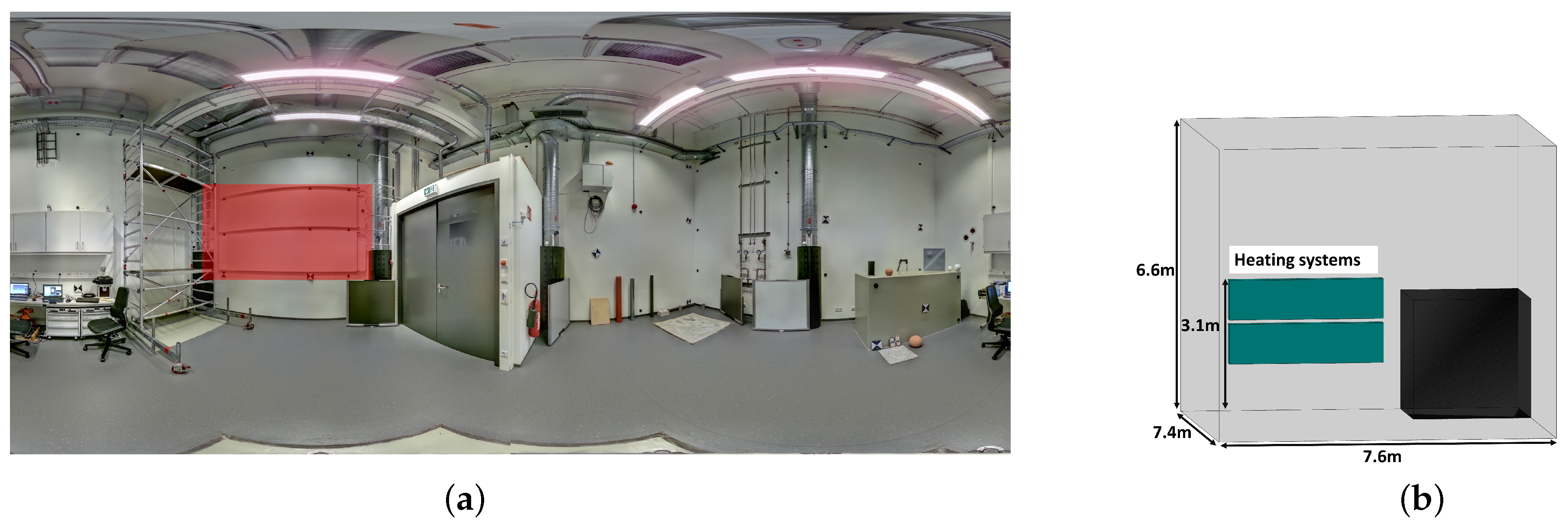
Figure 1. (a) Panoramic image from a single laser scan in the HiTec laboratory. Investigation of two heating systems (highlighted with the red rectangle). (b) Dimensions of the HiTec laboratory.
Remotesensing 15 02349 g001
Figure 2. (a) Targets used for registration: (1) Back of the TLS target. (2) Front of the TLS target. (3) Target mount for TLS and laser tracker targets. (4) Corner cube reflector for laser tracker measurement. (b) Section of the distribution of targets within the laboratory environment. The targets that are placed in the room are indicated by red rectangles.
Remotesensing 15 02349 g002
Figure 5. (a) Process chain: distance residual determination. (b) Principle of raycasting for distance residual calculation.
Remotesensing 15 02349 g005
Figure 6. Uncertainty factors of TLSs (in accordance with [23]).
Remotesensing 15 02349 g006
Figure 7. Correlation matrix between independent and dependent variables.
Remotesensing 15 02349 g007
Figure 8. Box plots of residuals over (a) intensity and (b) angle of impact. Blue boxes represent the 25 and 75 quantiles of the distribution. Red lines indicate the medians of the distribution. Green line indicates the fitted relationship between dependent and independent variables. Red crosses indicate outliers.
Remotesensing 15 02349 g008
Figure 9. Box plots of residuals over (a) distance, (b) spot size, and (c) curvature. Blue boxes represent the 25 and 75 quantiles of the distribution. Red line indicate the medians of the distribution. Red crosses indicate outliers.
Remotesensing 15 02349 g009
Figure 10. Histogram of residuals (a) and absolute residuals (b). Absolute residuals > 3 mm represent 0.28% of the data.
Remotesensing 15 02349 g010
Figure 11. Flowchart: XGBoost regressor.
Remotesensing 15 02349 g011
Figure 12. Hyperparameter search space for the three conventional approaches to optimize two hyperparameters.
Remotesensing 15 02349 g012
Figure 13. Flowchart: Training and validation process for the models.
Remotesensing 15 02349 g013
Figure 14. Partial dependencies plot for each model.
Remotesensing 15 02349 g014
Figure 15. Box plots of the trained parameter of the models. (a) Estimated weights for the linear model. (b) Estimated weights for the nonlinear model. (c) Feature importance for the XGBoost model. (d) Resulting hyperparameters from hyperparameter tuning. These parameters are used for training the XGBoost model.
Remotesensing 15 02349 g015
Figure 16. Validation results for test and validation data sets of the 3 trained models. (a) Coefficient of determination (higher is better). (b) RMSE (lower is better).
Remotesensing 15 02349 g016
Figure 17. Histogram of the residuals. (a) Effect of the prediction results on the residuals: after the calibration, the residuals are normally distributed. (b) Heat map of predicted residuals vs. actual residuals: the linear trend reveals a good fit.
Remotesensing 15 02349 g017
Figure 18. Calculated features for TLS point cloud. Intensity not scaled.
Remotesensing 15 02349 g018
Figure 19. (Left) Real residuals of the reference mesh. (Middle) Averaged predicted residuals from 120 XGBoost models. (Right) Residuals after calibration is applied to the distance measurement using the averaged predictions.
Remotesensing 15 02349 g019
Figure 20. Histogram of distance residuals before and after calibration.
Remotesensing 15 02349 g020
Figure 21. Standard deviation calculated using the 120 XGBoost prediction results.
Remotesensing 15 02349 g021
Table 1. Sensor characteristics [25,26,27]. Uncertainties of the Z+F Imager 5016 result from manufacturer’s calibration.
SensorSpecifications
Leica AT960 LRAngle accuracy: ±15  μ m + 6 μ m/m (Maximum permissible error)
Range accuracy: ±0.5  μ m/m (Maximum permissible error)
Measurement range (6 DoF): 40 m
Leica LAS XLMeasurement uncertainty plane surface: ±0.225 mm (one standard deviation)
Measurement range: 30 cm
Data acquisition rate: 143,000 pts/s
Z+F Imager 5016Vertical accuracy: 0 . 0021 = 0.04  mm/m (one standard deviation)
Horizontal accuracy: 0 . 0031 = 0.05  mm/m (one standard deviation)
Range noise: 0.16–0.2 mm (one standard deviation)
Measurement range: 0.3–365 m
Data acquisition rate: 1 mio. pts/s
Vertical resolution: 0 . 00026
Horiontal resolution: 0 . 00018
Table 2. Calculated features for all TLS points.
VariableFeatureUnitMinMaxMeanstd
x 0 Intensity-0.01311.0190.29330.1044
x 1 Angle of impactrad0.1741.5700.9520.323
x 2 Distancem0.55168.28932.09181.6516
x 3 Spot sizem0.00350.01020.00380.0003
x 4 Curvature-0.000000.000860.000330.00018
yDistance residualsm−0.01980.01950.000560.00073
Disclaimer/Publisher’s Note: The statements, opinions and data contained in all publications are solely those of the individual author(s) and contributor(s) and not of MDPI and/or the editor(s). MDPI and/or the editor(s) disclaim responsibility for any injury to people or property resulting from any ideas, methods, instructions or products referred to in the content.