


Reconstructing Digital Terrain Models from ArcticDEM and WorldView-2 Imagery in Livengood, Alaska


Abstract
1. Introduction
2. Methodology and Materials
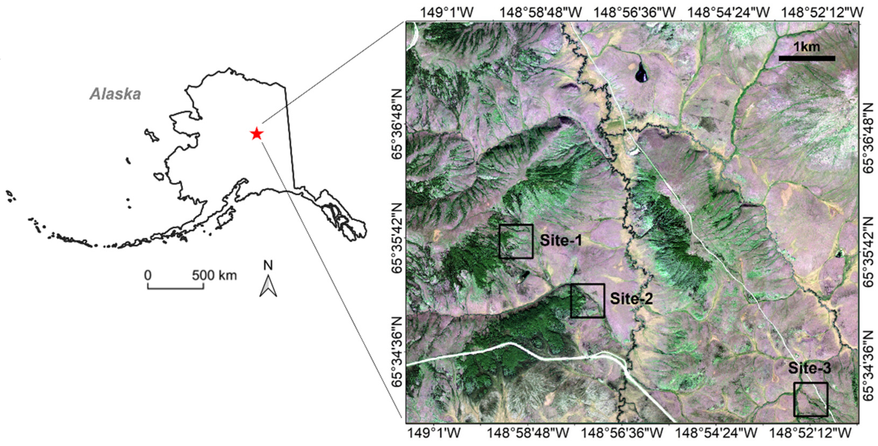
2.1. Study Sites and Data
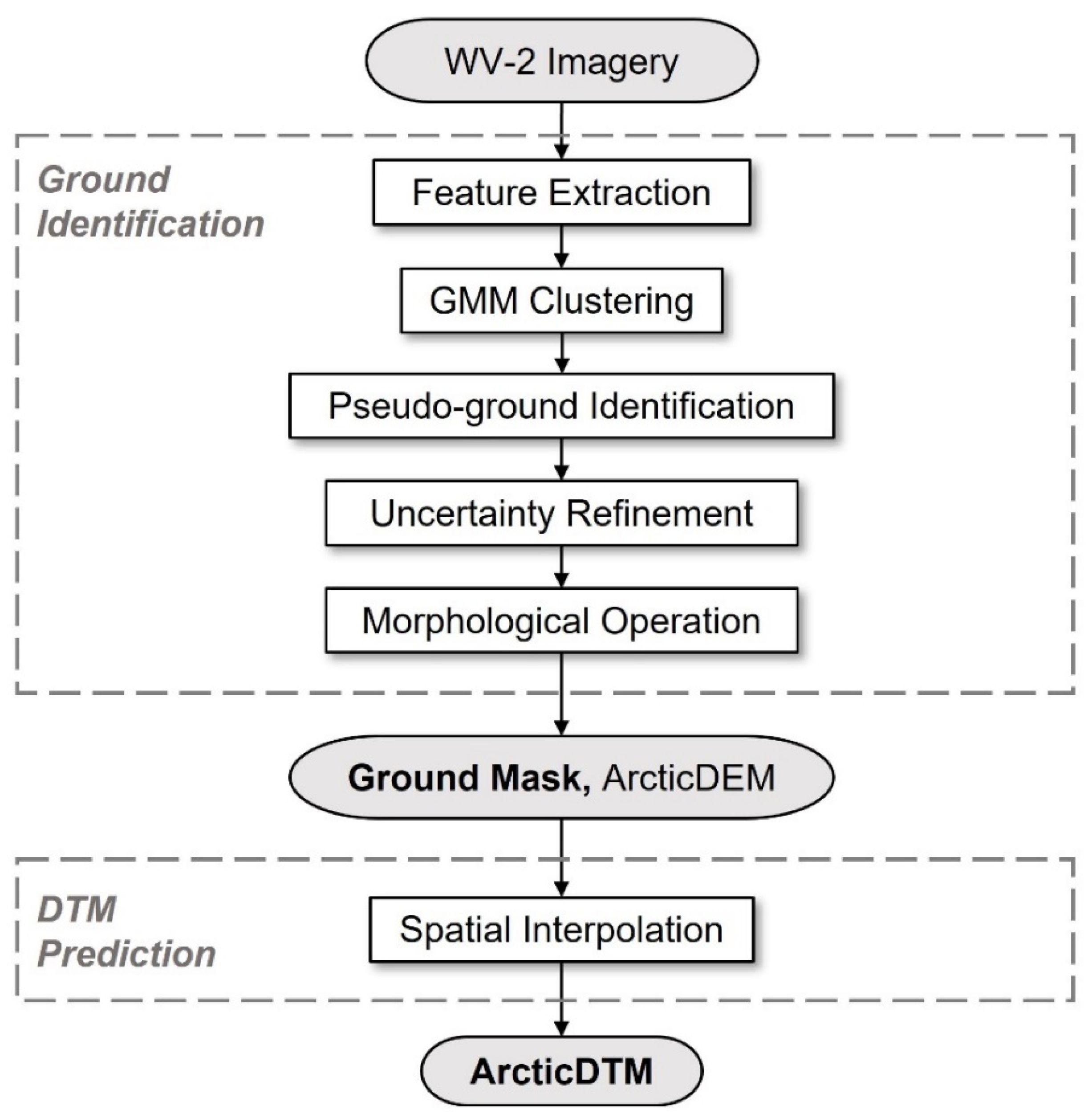
2.2. Proposed Method
2.2.1. Ground Identification
2.2.2. DTM Interpolation
2.3. Evaluation and Comparison
2.3.1. Ground Identification
2.3.2. DTM Interpolation
3. Results
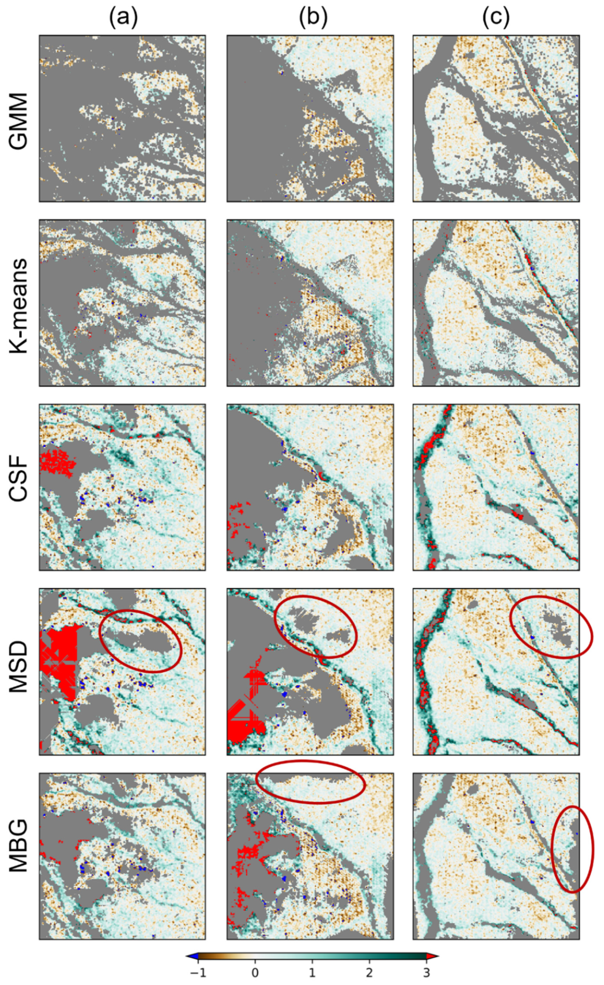
3.1. Ground Mask Extraction
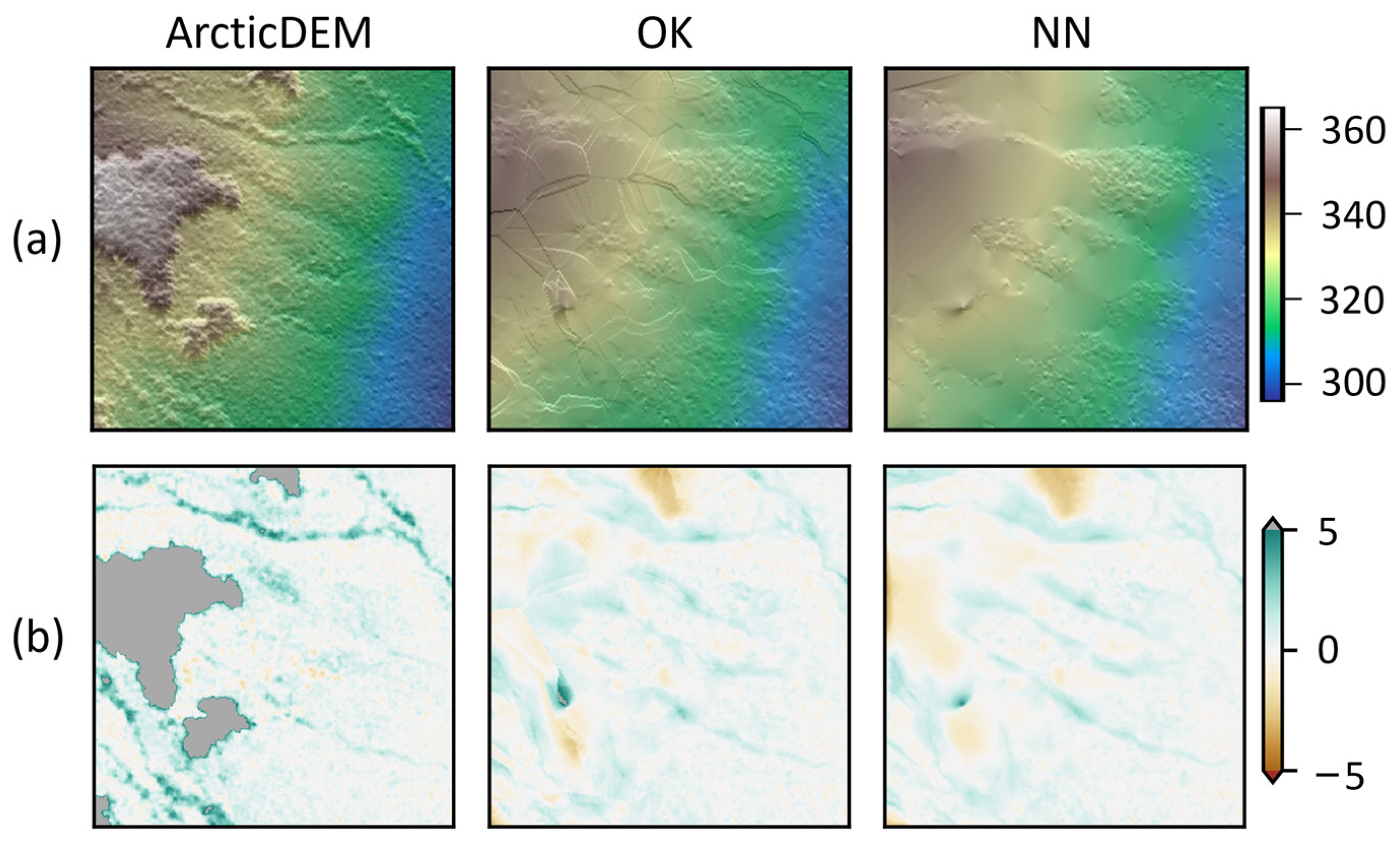
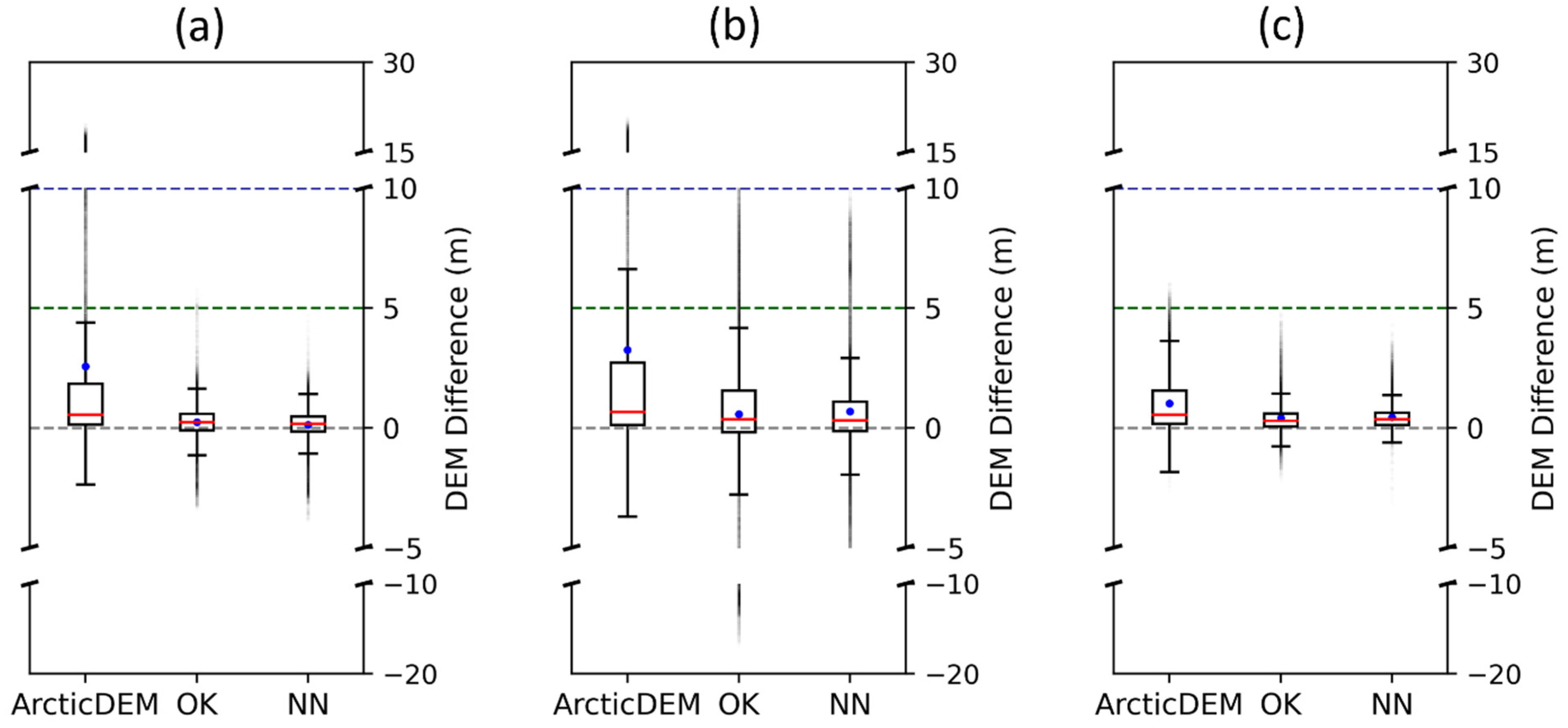
3.2. DTM Interpolation
4. Discussion
4.1. Ground Identification
4.2. Spatial Interpolation
4.3. Future Improvement
5. Conclusions
Author Contributions
Funding
Data Availability Statement
Acknowledgments
Conflicts of Interest
Appendix A

References
- Uysal, M.; Toprak, A.S.; Polat, N. DEM Generation with UAV Photogrammetry and Accuracy Analysis in Sahitler Hill. Measurement 2015, 73, 539–543. [Google Scholar] [CrossRef]
- Ariza-Villaverde, A.B.; Jiménez-Hornero, F.J.; De Ravé, E.G. Influence of DEM Resolution on Drainage Network Extraction: A Multifractal Analysis. Geomorphology 2015, 241, 243–254. [Google Scholar] [CrossRef]
- Delbridge, B.G.; Bürgmann, R.; Fielding, E.; Hensley, S.; Schulz, W.H. Three-Dimensional Surface Deformation Derived from Airborne Interferometric UAVSAR: Application to the Slumgullion Landslide. J. Geophys. Res. Solid Earth 2016, 121, 3951–3977. [Google Scholar] [CrossRef]
- Huang, M.-H.; Fielding, E.J.; Liang, C.; Milillo, P.; Bekaert, D.; Dreger, D.; Salzer, J. Coseismic Deformation and Triggered Landslides of the 2016 Mw 6.2 Amatrice Earthquake in Italy. Geophys. Res. Lett. 2017, 44, 1266–1274. [Google Scholar] [CrossRef]
- Akca, D.; Gruen, A.; Smagas, K.; Jimeno, E.; Stylianidis, E.; Altan, O.; Martin, V.S.; Garcia, A.; Poli, D.; Hofer, M. A Precision Estimation Method for Volumetric Changes. In Proceedings of the 2019 9th International Conference on Recent Advances in Space Technologies (RAST), Istanbul, Turkey, 11–14 June 2019; pp. 245–251. [Google Scholar]
- Tang, C.; Tanyas, H.; van Westen, C.J.; Tang, C.; Fan, X.; Jetten, V.G. Analysing Post-Earthquake Mass Movement Volume Dynamics with Multi-Source DEMs. Eng. Geol. 2019, 248, 89–101. [Google Scholar] [CrossRef]
- Guth, P.L.; Van Niekerk, A.; Grohmann, C.H.; Muller, J.-P.; Hawker, L.; Florinsky, I.V.; Gesch, D.; Reuter, H.I.; Herrera-Cruz, V.; Riazanoff, S.; et al. Digital Elevation Models: Terminology and Definitions. Remote Sens. 2021, 13, 3581. [Google Scholar] [CrossRef]
- Meddens, A.J.H.; Vierling, L.A.; Eitel, J.U.H.; Jennewein, J.S.; White, J.C.; Wulder, M.A. Developing 5 m Resolution Canopy Height and Digital Terrain Models from WorldView and ArcticDEM Data. Remote Sens. Environ. 2018, 218, 174–188. [Google Scholar] [CrossRef]
- Sadeghi, Y.; St-Onge, B.; Leblon, B.; Simard, M. Canopy Height Model (CHM) Derived from a TanDEM-X InSAR DSM and an Airborne Lidar DTM in Boreal Forest. IEEE J. Sel. Top. Appl. Earth Obs. Remote Sens. 2016, 9, 381–397. [Google Scholar] [CrossRef]
- Bolch, T.; Buchroithner, M.; Pieczonka, T.; Kunert, A. Planimetric and Volumetric Glacier Changes in the Khumbu Himal, Nepal, since 1962 Using Corona, Landsat TM and ASTER Data. J. Glaciol. 2008, 54, 592–600. [Google Scholar] [CrossRef]
- Kääb, A.; Vollmer, M. Surface Geometry, Thickness Changes and Flow Fields on Creeping Mountain Permafrost: Automatic Extraction by Digital Image Analysis. Permafr. Periglac. Process. 2000, 11, 315–326. [Google Scholar] [CrossRef]
- Erdogan, M.; Yilmaz, A. Detection of Building Damage Caused by Van Earthquake Using Image and Digital Surface Model (DSM) Difference. Int. J. Remote Sens. 2019, 40, 3772–3786. [Google Scholar] [CrossRef]
- Shen, D.; Qian, T.; Chen, W.; Chi, Y.; Wang, J. A Quantitative Flood-Related Building Damage Evaluation Method Using Airborne LiDAR Data and 2-D Hydraulic Model. Water 2019, 11, 987. [Google Scholar] [CrossRef]
- Noh, M.-J.; Howat, I.M. The Surface Extraction from TIN Based Search-Space Minimization (SETSM) Algorithm. ISPRS J. Photogramm. Remote Sens. 2017, 129, 55–76. [Google Scholar] [CrossRef]
- Barr, I.D.; Dokukin, M.D.; Kougkoulos, I.; Livingstone, S.J.; Lovell, H.; Małecki, J.; Muraviev, A.Y. Using ArcticDEM to Analyse the Dimensions and Dynamics of Debris-Covered Glaciers in Kamchatka, Russia. Geosciences 2018, 8, 216. [Google Scholar] [CrossRef]
- Dai, C.; Howat, I.M.; Freymueller, J.T.; Vijay, S.; Jia, Y. Characterization of the 2008 Phreatomagmatic Eruption of Okmok from ArcticDEM and InSAR: Deposition, Erosion, and Deformation. J. Geophys. Res. Solid Earth 2020, 125, e2019JB018977. [Google Scholar] [CrossRef]
- Dai, C.; Howat, I.M. Measuring Lava Flows with ArcticDEM: Application to the 2012–2013 Eruption of Tolbachik, Kamchatka. Geophys. Res. Lett. 2017, 44, 12–133. [Google Scholar] [CrossRef]
- Puliti, S.; Hauglin, M.; Breidenbach, J.; Montesano, P.; Neigh, C.S.R.; Rahlf, J.; Solberg, S.; Klingenberg, T.F.; Astrup, R. Modelling Above-Ground Biomass Stock over Norway Using National Forest Inventory Data with ArcticDEM and Sentinel-2 Data. Remote Sens. Environ. 2020, 236, 111501. [Google Scholar] [CrossRef]
- Dai, C.; Durand, M.; Howat, I.M.; Altenau, E.H.; Pavelsky, T.M. Estimating River Surface Elevation From ArcticDEM. Geophys. Res. Lett. 2018, 45, 3107–3114. [Google Scholar] [CrossRef]
- Xiao, C.; Qin, R.; Xie, X.; Huang, X. Individual Tree Detection and Crown Delineation with 3d Information from Multi-View Satellite Images. Photogramm. Eng. Remote Sens. 2019, 85, 55–63. [Google Scholar] [CrossRef]
- Zhang, W.; Qi, J.; Wan, P.; Wang, H.; Xie, D.; Wang, X.; Yan, G. An Easy-to-Use Airborne LiDAR Data Filtering Method Based on Cloth Simulation. Remote Sens. 2016, 8, 501. [Google Scholar] [CrossRef]
- Zeybek, M.; Şanlıoğlu, İ. Point Cloud Filtering on UAV Based Point Cloud. Measurement 2019, 133, 99–111. [Google Scholar] [CrossRef]
- Evans, J.S.; Hudak, A.T. A Multiscale Curvature Algorithm for Classifying Discrete Return LiDAR in Forested Environments. IEEE Trans. Geosci. Remote Sens. 2007, 45, 1029–1038. [Google Scholar] [CrossRef]
- Axelsson, P. DEM Generation from Laser Scanner Data Using Adaptive TIN Models. Int. Arch. Photogramm. Remote Sens. 2000, 33, 110–117. [Google Scholar]
- Meng, X.; Wang, L.; Silván-Cárdenas, J.L.; Currit, N. A Multi-Directional Ground Filtering Algorithm for Airborne LIDAR. ISPRS J. Photogramm. Remote Sens. 2009, 64, 117–124. [Google Scholar] [CrossRef]
- Perko, R.; Raggam, H.; Roth, P.M. Mapping with Pléiades—End-to-End Workflow. Remote Sens. 2019, 11, 2052. [Google Scholar] [CrossRef]
- Özcan, A.H.; Ünsalan, C.; Reinartz, P. Ground Filtering and DTM Generation from DSM Data Using Probabilistic Voting and Segmentation. Int. J. Remote Sens. 2018, 39, 2860–2883. [Google Scholar] [CrossRef]
- Pingel, T.J.; Clarke, K.C.; McBride, W.A. An Improved Simple Morphological Filter for the Terrain Classification of Airborne LIDAR Data. ISPRS J. Photogramm. Remote Sens. 2013, 77, 21–30. [Google Scholar] [CrossRef]
- Mongus, D.; Lukač, N.; Žalik, B. Ground and Building Extraction from LiDAR Data Based on Differential Morphological Profiles and Locally Fitted Surfaces. ISPRS J. Photogramm. Remote Sens. 2014, 93, 145–156. [Google Scholar] [CrossRef]
- Tian, J.; Krauss, T.; Reinartz, P. DTM Generation in Forest Regions from Satellite Stereo Imagery. Int. Arch. Photogramm. Remote Sens. Spat. Inf. Sci. 2014, 40, 401. [Google Scholar] [CrossRef]
- St-Onge, B.; Vega, C.; Fournier, R.A.; Hu, Y. Mapping Canopy Height Using a Combination of Digital Stereo-Photogrammetry and Lidar. Int. J. Remote Sens. 2008, 29, 3343–3364. [Google Scholar] [CrossRef]
- Agüera-Vega, F.; Agüera-Puntas, M.; Martínez-Carricondo, P.; Mancini, F.; Carvajal, F. Effects of Point Cloud Density, Interpolation Method and Grid Size on Derived Digital Terrain Model Accuracy at Micro Topography Level. Int. J. Remote Sens. 2020, 41, 8281–8299. [Google Scholar] [CrossRef]
- Bater, C.W.; Coops, N.C. Evaluating Error Associated with Lidar-Derived DEM Interpolation. Comput. Geosci. 2009, 35, 289–300. [Google Scholar] [CrossRef]
- Garnero, G.; Godone, D. Comparisons between Different Interpolation Techniques. Int. Arch. Photogramm. Remote Sens. Spat. Inf. Sci. 2013, 5, W3. [Google Scholar] [CrossRef]
- Ghandehari, M.; Buttenfield, B.P.; Farmer, C.J.Q. Comparing the Accuracy of Estimated Terrain Elevations across Spatial Resolution. Int. J. Remote Sens. 2019, 40, 5025–5049. [Google Scholar] [CrossRef]
- Guo, Q.; Li, W.; Yu, H.; Alvarez, O. Effects of Topographic Variability and Lidar Sampling Density on Several DEM Interpolation Methods. Photogramm. Eng. Remote Sens. 2010, 76, 701–712. [Google Scholar] [CrossRef]
- Chen, C.; Li, Y. A Fast Global Interpolation Method for Digital Terrain Model Generation from Large LiDAR-Derived Data. Remote Sens. 2019, 11, 1324. [Google Scholar] [CrossRef]
- Meng, X.; Lin, Y.; Yan, L.; Gao, X.; Yao, Y.; Wang, C.; Luo, S. Airborne LiDAR Point Cloud Filtering by a Multilevel Adaptive Filter Based on Morphological Reconstruction and Thin Plate Spline Interpolation. Electronics 2019, 8, 1153. [Google Scholar] [CrossRef]
- Razak, K.A.; Santangelo, M.; Van Westen, C.J.; Straatsma, M.W.; de Jong, S.M. Generating an Optimal DTM from Airborne Laser Scanning Data for Landslide Mapping in a Tropical Forest Environment. Geomorphology 2013, 190, 112–125. [Google Scholar] [CrossRef]
- Stereńczak, K.; Ciesielski, M.; Balazy, R.; Zawiła-Niedźwiecki, T. Comparison of Various Algorithms for DTM Interpolation from LIDAR Data in Dense Mountain Forests. Eur. J. Remote Sens. 2016, 49, 599–621. [Google Scholar] [CrossRef]
- Viereck, L.A.; Little, E.L. Alaska Trees and Shrubs; US Forest Service: Washington, DC, USA, 1972.
- Porter, C.; Morin, P.; Howat, I.; Noh, M.-J.; Bates, B.; Peterman, K.; Keesey, S.; Schlenk, M.; Gardiner, J.; Tomko, K.; et al. ArcticDEM. version 3. 2018; Harvard Dataverse, V1. [Google Scholar] [CrossRef]
- Hubbard, T.D.; Koehler, R.D.; Combellick, R.A. High-Resolution Lidar Data for Alaska Infrastructure Corridors; Alaska Division of Geological & Geophysical Surveys: Fairbanks, AK, USA, 2011; Volume 3, p. 291. [CrossRef]
- Rusinkiewicz, S.; Levoy, M. Efficient Variants of the ICP Algorithm. In Proceedings of the Third International Conference on 3-D Digital Imaging and Modeling, Quebec City, QC, Canada, 28 May–1 June 2001; pp. 145–152. [Google Scholar]
- McLachlan, G.J.; Basford, K.E. Mixture Models. Inference and Applications to Clustering; Dekker: New York, NY, USA, 1988. [Google Scholar]
- Raykov, Y.P.; Boukouvalas, A.; Baig, F.; Little, M.A. What to Do When K-Means Clustering Fails: A Simple yet Principled Alternative Algorithm. PLoS ONE 2016, 11, e0162259. [Google Scholar] [CrossRef]
- Biernacki, C.; Celeux, G.; Govaert, G. Assessing a Mixture Model for Clustering with the Integrated Completed Likelihood. IEEE Trans. Pattern Anal. Mach. Intell. 2000, 22, 719–725. [Google Scholar] [CrossRef]
- McLachlan, G.J.; Peel, D. Finite Mixture Models; John Wiley & Sons: Hoboken, NJ, USA, 2004; ISBN 978-0-471-65406-3. [Google Scholar]
- Pedregosa, F.; Varoquaux, G.; Gramfort, A.; Michel, V.; Thirion, B.; Grisel, O.; Blondel, M.; Prettenhofer, P.; Weiss, R.; Dubourg, V. Scikit-Learn: Machine Learning in Python. J. Mach. Learn. Res. 2011, 12, 2825–2830. [Google Scholar]
- Bailey, T.L.; Elkan, C. Fitting a Mixture Model by Expectation Maximization to Discover Motifs in Bipolymers. Proc. Int. Conf. Intell. Syst. Mol. Biol. 1994, 2, 28–36. [Google Scholar] [PubMed]
- Schwarz, G. Estimating the Dimension of a Model. Ann. Stat. 1978, 6, 461–464. [Google Scholar] [CrossRef]
- Qi, J.; Chehbouni, A.; Huete, A.R.; Kerr, Y.H.; Sorooshian, S. A Modified Soil Adjusted Vegetation Index. Remote Sens. Environ. 1994, 48, 119–126. [Google Scholar] [CrossRef]
- McFeeters, S.K. The Use of the Normalized Difference Water Index (NDWI) in the Delineation of Open Water Features. Int. J. Remote Sens. 1996, 17, 1425–1432. [Google Scholar] [CrossRef]
- Cressie, N. Spatial Prediction and Ordinary Kriging. Math. Geol. 1988, 20, 405–421. [Google Scholar] [CrossRef]
- Zhu, X.; Liu, D.; Chen, J. A New Geostatistical Approach for Filling Gaps in Landsat ETM+ SLC-off Images. Remote Sens. Environ. 2012, 124, 49–60. [Google Scholar] [CrossRef]
- Tily, R.; Brace, C.J. A Study of Natural Neighbour Interpolation and Its Application to Automotive Engine Test Data. Proc. Inst. Mech. Eng. Part J. Automob. Eng. 2006, 220, 1003–1017. [Google Scholar] [CrossRef]
- Pebesma, E.J. Multivariable Geostatistics in S: The Gstat Package. Comput. Geosci. 2004, 30, 683–691. [Google Scholar] [CrossRef]
- Ribeiro, P.J., Jr.; Diggle, P.J. GeoR: A Package for Geostatistical Analysis. R News 2001, 1, 14–18. [Google Scholar]
- Barsi, Á.; Kugler, Z.; László, I.; Szabó, G.; Abdulmutalib, H.M. Accuracy Dimensions in Remote Sensing. Int. Arch. Photogramm. Remote Sens. Spat. Inf. Sci. 2018, XLII-3, 61–67. [Google Scholar] [CrossRef]
- DeWitt, J.D.; Warner, T.A.; Chirico, P.G.; Bergstresser, S.E. Creating High-Resolution Bare-Earth Digital Elevation Models (DEMs) from Stereo Imagery in an Area of Densely Vegetated Deciduous Forest Using Combinations of Procedures Designed for Lidar Point Cloud Filtering. GISci. Remote Sens. 2017, 54, 552–572. [Google Scholar] [CrossRef]
- McDaniel, M.W.; Nishihata, T.; Brooks, C.A.; Salesses, P.; Iagnemma, K. Terrain Classification and Identification of Tree Stems Using Ground-Based LiDAR. J. Field Robot. 2012, 29, 891–910. [Google Scholar] [CrossRef]
- Scott, G.J.; England, M.R.; Starms, W.A.; Marcum, R.A.; Davis, C.H. Training Deep Convolutional Neural Networks for Land–Cover Classification of High-Resolution Imagery. IEEE Geosci. Remote Sens. Lett. 2017, 14, 549–553. [Google Scholar] [CrossRef]
- Bandara, K.R.M.U.; Samarakoon, L.; Shrestha, R.P.; Kamiya, Y. Automated Generation of Digital Terrain Model Using Point Clouds of Digital Surface Model in Forest Area. Remote Sens. 2011, 3, 845–858. [Google Scholar] [CrossRef]
- Montesano, P.M.; Neigh, C.; Sun, G.; Duncanson, L.; Van Den Hoek, J.; Ranson, K.J. The Use of Sun Elevation Angle for Stereogrammetric Boreal Forest Height in Open Canopies. Remote Sens. Environ. 2017, 196, 76–88. [Google Scholar] [CrossRef]
- Vastaranta, M.; Yu, X.; Luoma, V.; Karjalainen, M.; Saarinen, N.; Wulder, M.A.; White, J.C.; Persson, H.J.; Hollaus, M.; Yrttimaa, T.; et al. Aboveground Forest Biomass Derived Using Multiple Dates of WorldView-2 Stereo-Imagery: Quantifying the Improvement in Estimation Accuracy. Int. J. Remote Sens. 2018, 39, 8766–8783. [Google Scholar] [CrossRef]
- Abdalati, W.; Zwally, H.J.; Bindschadler, R.; Csatho, B.; Farrell, S.L.; Fricker, H.A.; Harding, D.; Kwok, R.; Lefsky, M.; Markus, T.; et al. The ICESat-2 Laser Altimetry Mission. Proc. IEEE 2010, 98, 735–751. [Google Scholar] [CrossRef]
- Cartus, O.; Kellndorfer, J.; Rombach, M.; Walker, W. Mapping Canopy Height and Growing Stock Volume Using Airborne Lidar, ALOS PALSAR and Landsat ETM+. Remote Sens. 2012, 4, 3320–3345. [Google Scholar] [CrossRef]
- Urbazaev, M.; Cremer, F.; Migliavacca, M.; Reichstein, M.; Schmullius, C.; Thiel, C. Potential of Multi-Temporal ALOS-2 PALSAR-2 ScanSAR Data for Vegetation Height Estimation in Tropical Forests of Mexico. Remote Sens. 2018, 10, 1277. [Google Scholar] [CrossRef]
- Bartsch, A.; Widhalm, B.; Leibman, M.; Ermokhina, K.; Kumpula, T.; Skarin, A.; Wilcox, E.J.; Jones, B.M.; Frost, G.V.; Höfler, A.; et al. Feasibility of Tundra Vegetation Height Retrieval from Sentinel-1 and Sentinel-2 Data. Remote Sens. Environ. 2020, 237, 111515. [Google Scholar] [CrossRef]
- Carreiras, J.M.; Quegan, S.; Le Toan, T.; Minh, D.H.T.; Saatchi, S.S.; Carvalhais, N.; Reichstein, M.; Scipal, K. Coverage of High Biomass Forests by the ESA BIOMASS Mission under Defense Restrictions. Remote Sens. Environ. 2017, 196, 154–162. [Google Scholar] [CrossRef]
- Aguilar, F.J.; Agüera, F.; Aguilar, M.A.; Carvajal, F. Effects of Terrain Morphology, Sampling Density, and Interpolation Methods on Grid DEM Accuracy. Photogramm. Eng. Remote Sens. 2005, 71, 805–816. [Google Scholar] [CrossRef]
- Šiljeg, A.; Barada, M.; Marić, I.; Roland, V. The Effect of User-Defined Parameters on DTM Accuracy—Development of a Hybrid Model. Appl. Geomat. 2019, 11, 81–96. [Google Scholar] [CrossRef]


| Method | TP | TI | TII | OA | F1 | |
|---|---|---|---|---|---|---|
| Site-1 | GMM | 0.129 | 0.413 | 0.682 | 0.634 | 0.413 |
| K-means | 0.268 | 0.458 | 0.336 | 0.637 | 0.597 | |
| CSF | 0.374 | 0.524 | 0.074 | 0.558 | 0.629 | |
| MSD | 0.351 | 0.555 | 0.132 | 0.508 | 0.588 | |
| MBG | 0.338 | 0.497 | 0.165 | 0.600 | 0.628 | |
| Site-2 | GMM | 0.263 | 0.288 | 0.395 | 0.722 | 0.654 |
| K-means | 0.333 | 0.383 | 0.234 | 0.691 | 0.683 | |
| CSF | 0.359 | 0.437 | 0.173 | 0.646 | 0.670 | |
| MSD | 0.332 | 0.484 | 0.236 | 0.587 | 0.616 | |
| MBG | 0.361 | 0.467 | 0.169 | 0.610 | 0.649 | |
| Site-3 | GMM | 0.389 | 0.314 | 0.306 | 0.651 | 0.690 |
| K-means | 0.489 | 0.355 | 0.126 | 0.66 | 0.742 | |
| CSF | 0.537 | 0.421 | 0.041 | 0.587 | 0.722 | |
| MSD | 0.538 | 0.434 | 0.039 | 0.566 | 0.712 | |
| MBG | 0.499 | 0.386 | 0.109 | 0.626 | 0.727 |
| Method | RMSE (m) | rRMSE | MAE (m) | ME (m) | |
|---|---|---|---|---|---|
| Site-1 | GMM | 0.328 | 0.006 | 0.250 | 0.058 |
| K-means | 0.538 | 0.010 | 0.339 | 0.174 | |
| CSF | 2.516 | 0.047 | 0.836 | 0.689 | |
| MSD | 4.000 | 0.074 | 1.576 | 1.443 | |
| MBG | 0.867 | 0.016 | 0.438 | 0.267 | |
| Site-2 | GMM | 0.343 | 0.005 | 0.256 | 0.039 |
| K-means | 0.635 | 0.010 | 0.350 | 0.143 | |
| CSF | 1.467 | 0.023 | 0.534 | 0.347 | |
| MSD | 3.350 | 0.052 | 1.272 | 1.099 | |
| MBG | 2.411 | 0.037 | 0.812 | 0.603 | |
| Site-3 | GMM | 0.348 | 0.006 | 0.233 | 0.047 |
| K-means | 0.522 | 0.009 | 0.305 | 0.146 | |
| CSF | 0.780 | 0.014 | 0.442 | 0.306 | |
| MSD | 0.880 | 0.016 | 0.510 | 0.378 | |
| MBG | 0.432 | 0.008 | 0.298 | 0.146 |
| Method | RMSE (m) | rRMSE | MAE (m) | ME (m) | LE (%) | UE (%) |
|---|---|---|---|---|---|---|
| ArcticDEM | 4.722 | 0.088 | 2.136 | 2.015 | 0.000 | 19.282 |
| OK | 0.677 | 0.013 | 0.470 | 0.195 | 0.101 | 0.288 |
| NN | 0.648 | 0.012 | 0.449 | 0.113 | 0.154 | 0.054 |
| Method | RMSE (m) | rRMSE | MAE (m) | ME (m) | LE (%) | UE (%) |
|---|---|---|---|---|---|---|
| ArcticDEM | 4.841 | 0.075 | 2.106 | 1.939 | 0.015 | 24.104 |
| OK | 3.028 | 0.047 | 1.459 | 0.354 | 8.277 | 15.318 |
| NN | 1.677 | 0.026 | 0.87 | 0.423 | 3.229 | 8.734 |
| Method | RMSE (m) | rRMSE | MAE (m) | ME (m) | LE (%) | UE (%) |
|---|---|---|---|---|---|---|
| ArcticDEM | 1.071 | 0.019 | 0.594 | 0.467 | 0.000 | 9.487 |
| OK | 0.563 | 0.010 | 0.353 | 0.203 | 0.000 | 0.902 |
| NN | 0.521 | 0.009 | 0.342 | 0.221 | 0.005 | 0.326 |
Disclaimer/Publisher’s Note: The statements, opinions and data contained in all publications are solely those of the individual author(s) and contributor(s) and not of MDPI and/or the editor(s). MDPI and/or the editor(s) disclaim responsibility for any injury to people or property resulting from any ideas, methods, instructions or products referred to in the content. |
© 2023 by the authors. Licensee MDPI, Basel, Switzerland. This article is an open access article distributed under the terms and conditions of the Creative Commons Attribution (CC BY) license (https://creativecommons.org/licenses/by/4.0/).
Share and Cite
Zhang, T.; Liu, D. Reconstructing Digital Terrain Models from ArcticDEM and WorldView-2 Imagery in Livengood, Alaska. Remote Sens. 2023, 15, 2061. https://doi.org/10.3390/rs15082061
Zhang T, Liu D. Reconstructing Digital Terrain Models from ArcticDEM and WorldView-2 Imagery in Livengood, Alaska. Remote Sensing. 2023; 15(8):2061. https://doi.org/10.3390/rs15082061
Chicago/Turabian StyleZhang, Tianqi, and Desheng Liu. 2023. "Reconstructing Digital Terrain Models from ArcticDEM and WorldView-2 Imagery in Livengood, Alaska" Remote Sensing 15, no. 8: 2061. https://doi.org/10.3390/rs15082061
APA StyleZhang, T., & Liu, D. (2023). Reconstructing Digital Terrain Models from ArcticDEM and WorldView-2 Imagery in Livengood, Alaska. Remote Sensing, 15(8), 2061. https://doi.org/10.3390/rs15082061