Article

Improving Smartphone GNSS Positioning Accuracy Using Inequality Constraints

1
School of Transportation, Southeast University, Nanjing 210096, China
2
Department of Geomatics Engineering, University of Calgary, Calgary, AB T2N 1N4, Canada
*
Author to whom correspondence should be addressed.
Remote Sens. 2023, 15(8), 2062; https://doi.org/10.3390/rs15082062
Submission received: 18 February 2023 / Revised: 4 April 2023 / Accepted: 11 April 2023 / Published: 13 April 2023
(This article belongs to the Special Issue GNSS Advanced Positioning Algorithms and Innovative Applications)

Abstract

:
To improve smartphone GNSS positioning performance using extra inequality information, an inequality constraint method was introduced and verified in this study. Firstly, the positioning model was reviewed and three constraint applications were derived from it, namely, vertical velocity, direction, and distance constraints. Secondly, we introduced an estimator based on the density function truncation method to solve the inequality constraint problem. Finally, the performance of the method was investigated using datasets from three smartphones, including a Huawei P30, a Huawei P40, and a Xiaomi MI8. The results indicate that the position and velocity accuracy can be improved in the up component using a vertical velocity constraint. The horizontal positioning accuracy was increased using a heading direction constraint with dynamic datasets. Numerically, the root mean square error (RMSE) improvement percentages were 16.77%, 14.57%, and 31.09% for HP40, HP30, and XMI8, respectively. Using an inter-smartphone distance constraint could enhance the horizontal positioning of all participating smartphones, with improvement percentages of 34.27%, 75.58%, and 23.66% for HP40, HP30, and XMI8, respectively, in the static dataset. Additionally, the improvement percentages were 15.90%, 5.55%, and 0.17% in dynamic datasets. In summary, this study demonstrates that utilizing inequality constraints can significantly improve smartphone GNSS positioning.

Graphical Abstract

1. Introduction

In 2016, Google announced that raw Global Navigation Satellite System (GNSS) observations including carrier phase measurements would be accessible to developers, providing more opportunities for the implementation of location-based services (LBS) on smartphones [1]. Extensive studies have been conducted to develop different data processing and positioning algorithms for achieving precise smartphone-based location tracking [2,3].
Numerous studies have investigated both absolute positioning and relative positioning algorithms for smartphones. Banville et al. initially evaluated the single-point positioning (SPP) performance of the Samsung Galaxy S7 using only GPS single-frequency pseudo-range observations, and the results indicated that the smartphone was capable of providing only meter-level accuracy [4]. To improve code-based positioning performance, carrier smooth code (CSC) or Doppler smooth code (DSC) approaches have been proposed, which take advantage of the high-precision carrier phase measurements available on some smartphones [5]. Geng et al. combined pseudo-range, carrier phase, and Doppler observations using an improved Hatch filter, proposing an algorithm called the three-thresholds and single-difference Hatch filter (TT-SD filter), which achieved sub-meter-level positioning accuracy [6]. Zhang et al. proposed an algorithm based on the time-differenced carrier phase (TDCP) filter, which obtained meter-level accuracy [7]. Precise point positioning (PPP) is another important algorithm in absolute positioning, and several studies have investigated its application in smartphones capable of performing carrier phase measurements [8]. These investigations also considered data analysis, observation processing, and model modification [9,10,11], and the results confirmed that sub-meter-level accuracy in static scenarios and meter-level accuracy in kinematics are achievable on smartphones using the PPP algorithm [12]. In addition to absolute positioning, relative positioning methods are also frequently studied, with real-time kinematics (RTK) being a major approach [13]. In short-baseline cases, atmospheric delay can be eliminated, allowing the RTK algorithm to provide high-precision location estimates [14]. Investigations using different smartphone brands and various use cases have consistently demonstrated the feasibility of achieving high-precision positioning using certain types of smartphone.
The aforementioned studies have primarily focused on smartphone positioning that relies on GNSS observations obtained from the smartphone’s application programming interface (API). However, considering that smartphones are equipped with multiple sensors, additional measurements can be obtained, which can be used as constraints in positioning algorithms to improve positioning accuracy and stability [15]. Several studies have been conducted to verify the performance of GNSS combined with other sensor information on smartphones to enhance positioning accuracy [16]. For example, it has been demonstrated that combining GNSS and Inertial Navigation System (INS) measurements in a loosely coupled manner can significantly improve smartphone location accuracy [17,18]. Other observation constraints, such as camera observations, digital map data, and WiFi signals, have also been investigated [19,20,21]. In most cases, the additional information is expressed as an equality constraint. However, in some scenarios, it is more appropriate to express the range information as an inequality constraint [22]. For example, a smartphone can compute road direction based on node positions, which are obtained from digital maps, but this information alone may not accurately indicate the actual direction of a vehicle [23]. Thus, expressing the range of direction as an inequality constraint can provide better results. Similarly, although smartphone collaborative positioning (CP) using inter-device distance has been investigated in several studies [24,25,26], it is uncommon to express the distance as an inequality constraint while taking into account vehicle length information. Therefore, it is crucial to explore methods that can utilize range information as an inequality constraint to further improve smartphone positioning accuracy.
In this study, we aim to improve the accuracy of smartphone positioning using range information via an inequality constraint estimation approach. Simon et al. previously demonstrated that the error variance of a solution obtained through inequality-constrained state estimation is equal to or less than that of a solution obtained through unconstrained estimation [27]. Various methods have been proposed to solve the inequality constraint problem, such as the active sets method, the Bayesian method, and the projection method [27,28,29]. However, it has been noted that projecting state estimates onto the constraint hyperplane does not necessarily place the mean of the state near the mean of the feasible region [30]. As such, we choose the probability density truncation (PDF) method as our estimator, which updates the state with the mean and covariance of the PDF region [31]. Additionally, an iterative procedure is used to ensure that the probability within the constraint range exceeds a given threshold. To validate our method, we introduce three applications: vertical velocity constraint, direction constraint, and inter-smartphone distance constraint. The structures of these constraints are introduced, and their effectiveness is demonstrated in the experimental section.
The rest of the paper is organized as follows. Firstly, the positioning model is reviewed, and then we introduce the design of the inequality constraint matrices in different applications. Secondly, the density function truncation method is introduced in detail, including the estimator and the iterative procedure. Thirdly, the performance of the method is analyzed using a real-world collection of datasets from three smartphones. Finally, we conclude the paper.

2. Positioning Model and Inequality Constraints

In this section, the positioning model on Android smartphones is introduced. Additionally, we describe the constraint matrices of three different applications.

2.1. Positioning Model for Android Smartphones

The pseudo-range, carrier phase, and Doppler measurements between satellite s and smartphone r with regard to frequency i can be expressed as follows [32,33]:
P r , i s = ρ r s + c d t r d T s + I r , i s + T r s + d r , i d i s + m r , i s + ϵ P r , i s Φ r , i s = ρ r s + c d t r d T s I r , i s + T r s + λ i ϕ r , 0 , i ϕ 0 , i s + N r , i s + δ r , i δ i s + M r , i s + d Φ r , i s + ϵ Φ r , i s λ i D r , i s = ρ ˙ r s + c d t ˙ r d T ˙ s + I ˙ r , i s + T ˙ r s + M ˙ r , i s + ϵ D r , i s
where P r , i s , Φ r , i s , and λ i D r , i s represent the pseudo-range, carrier phase, and Doppler observations in meters, respectively. i represents frequency, and λ i indicates the wavelength under the frequency. ρ r s represents the distance between the smartphone and the satellite in meters, ρ r s ˙   is its change rate in m / s , d t r and d T s indicate the receiver and satellite clock offset, d t ˙ r and d T ˙ s represent the change rate of the receiver and satellite clock offset, and c represents light speed. I r , i s and T r s represent the ionospheric delay and tropospheric delay, I ˙ r , i s and T ˙ r s represent their change rates, d r , i   and d i s represent the smartphone and satellite pseudo-range hardware delay, m r , i s represents the pseudo-range multipath delay, and ϕ r , 0 , i and ϕ 0 , i s represent the initial phase of the smartphone and the satellite, respectively. N r , i s represents the integer ambiguity in the unit of cycle [33]. δ r , j and δ s represent the receiver and satellite hardware delay of the carrier phase observation, M r , i s represents the carrier multipath error, and M ˙ r , i s represents its change rate. d Φ r , i s represents the carrier phase correction term, which includes phase center offsets, Earth tides, and relativity corrections, and ϵ P r , i s , ϵ Φ r , i s , and ϵ D r , i s represent the noise of the pseudo-range, carrier phase, and Doppler observations.
For some types of smartphone, such as Xiaomi 9 or Xiaomi 10, the carrier observation cannot be obtained from the API, and the RTK or PPP method is inapplicable [34,35]. In this case, the positioning algorithms that are based on pseudo-range observations, such as the SPP algorithm or the real-time differential (RTD) algorithm, are practical [36]. In this paper, we apply pseudo-range measurements for positioning. In addition, we use the inter-smartphone observations differential to eliminate the smartphone clock offset [6]. Overall, the estimated variables are given below [5]:
X = r v α
where r = x y z T , v = v x v y v z T , and α = α x α y α z T represent vectors, including their positions, in meters, velocity in m / s , and acceleration in m / s 2 , respectively. T represents vector transposition.

2.2. Inequality Constraint Model

In a poor observation environment, taking actual information into consideration will make the positioning model more reliable. In this paper, we apply a vertical velocity constraint, direction constraint, and inter-smartphone distance constraint to enhance the position estimation. Typically, the inequality constraint method is employed, and the state inequality relationships can be presented in a linear form, as follows:
C X d
where C represents the constraint matrix, d represents a vector that contains the threshold, and denotes that each element in the left vector ( C X ) is smaller than or equal to the corresponding elements in the right vector ( d ).

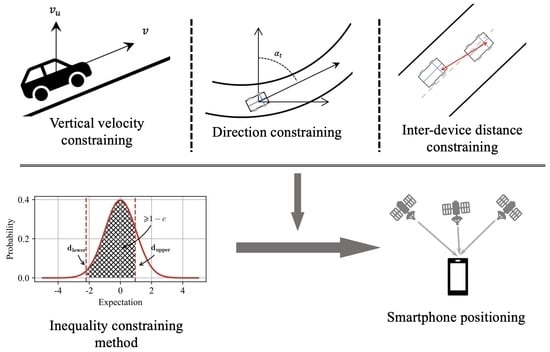
2.2.1. Vertical Velocity Constraint

Because of the limitation of road slope and the velocity of vehicles, there could be an upper bound of velocity in the up component. For instance, the Highway Technique Standard has a speed limitation of 120 km/h and a slope limitation of 3% on highways [37]; in this case, the range of the vertical velocity should be −1 m/s~1 m/s. In other words, even if the horizontal velocity of smartphones is unknown, we can still set an empirical threshold for vertical velocity in most cases. In this part, the threshold is expressed using the following inequation:
v u σ u
where v u   represents vertical velocity, and σ u represent the threshold in m / s . Note that this inequation is established under the body system and is not directly applicable. We must first convert the results from the WGS84 system to the body system. In addition, considering that after constraining the position can be changed, iteration is necessary for the results to fit the velocity inequation condition. To avoid complex and low-efficiency iteration procedures, we transform velocity into position change. Assuming that the interval is Δ t , we can calculate the height constraints of continuous epochs as follows:
σ h = σ u × Δ t
where σ h represents the threshold of the height change in meters, and Δ t represents the sampling interval in seconds. In this paper, the sampling interval is 1 s. Additionally, the vertical velocity constraint can be converted as follows:
h t + 1 h t σ h
where t and t + 1 represent different epochs, h t + 1 and h t represent the height in two epochs. Regarding coordinate system conversion, we can choose a position p 0 near the smartphone as the reference, and this position can be calculated using the SPP algorithm. The transform matrix can be computed as follows based on the reference p 0 :
E 0 = sin l cos l 0 sin b cos l sin b sin l cos b cos b cos l cos b sin l sin b
where E 0 represents the conversion matrix, and b and l represent the latitude and longitude of the reference p 0 . With this conversion matrix, we can compute the height difference of continuous epochs as follows:
h t + 1 h t = cos b cos l cos b sin l sin b r t + 1 r t
It should be noted that only the third row in E 0 is selected since only the height component is applied. In addition, considering that the symbol of absolute value is utilized in Equation (6), we can express the inequation as follows:
cos b cos l cos b sin l sin b r t + 1 r t σ h cos b cos l cos b sin l sin b r t + 1 r t σ h
The change in position between continuous epochs can be computed using the velocity, the acceleration, and the sampling interval. The position in the above inequality can be written as:
r t + 1 r t = v t Δ t + 0.5 α t Δ t 2
Overall, upon applying the empirical vertical velocity information, we can establish the constraint matrix as follows:
E ¯ 0 = cos b cos l cos b sin l sin b cos b cos l cos b sin l sin b C 0 = 0 2 × 3 E ¯ 0 Δ t 0.5 E ¯ 0 Δ t 2 d 0 = σ h σ h T
where E ¯ 0 represents the third row of E 0 , C 0 and d 0 are the constraint matrices. Additionally, we obtain the following inequality:
C 0 X d 0

2.2.2. Direction Constraint

In some cases, the moving direction of a smartphone or vehicle can be obtained. For instance, its direction can be calculated by the road nodes in a digital map, such as the Open Street Map (OSM), which can be downloaded onto a smartphone. An example is given below, with some of the elements of an OSM shown in Figure 1. In this figure, the black lines represent roads, and the red points represent the nodes of the roads. The latitude and longitude of the four nodes are given in Table 1. Assuming that the vehicle moved from east to west, we can calculate the direction: α D A = 260.48 ° , and α B C = 248.59 ° . Additionally, this information can be used as constraints in a positioning campaign.
We can set a range when applying direction information. Additionally, we can employ the position change in the body system to estimate direction. The direction constraint at this stage can be written as follows:
tan 1 Δ x e t Δ x n t α t δ
where α t represents the prior direction, and δ represents the threshold, which is determined by the tolerance range of the direction. Δ x e t and Δ x n t represent the east and north position changes in meters. Similar to Equation (8), they can be calculated as follows:
Δ x e t = sin l cos l 0 r t + 1 r t Δ x n t = sin b cos l sin b sin l cos b r t + 1 r t
This is an inverse trigonometric function and a fraction in Equation (13). It is difficult to convert this inequality into a linear form. In this paper, we propose several steps to achieve the above direction inequality constraint. In the first step, we can compute the initial direction using the unconstrained position results. If the direction is within the given range, the constraint is not necessary. If the direction is outside the range, we proceed to the second step, in which we convert the position change result from the body system to a new coordinate system, as shown in Figure 2. As shown in the figure, the direction can be limited to a range of δ ~ δ after conversion. Additionally, the rotation method is introduced in Equation (15).
Δ x ^ e t Δ x ^ n t = cos α t sin α t sin α t cos α t Δ x e t Δ x n t
In Equation (15), Δ x ^ e t and Δ x ^ n t represent the converted position change. A new inequality can be obtained as follows:
δ tan 1 Δ x ^ e t Δ x ^ n t δ
Assuming that δ is smaller than π / 2 , we can obtain the inequality in linear form as follows:
Δ x ^ n t 0 Δ x ^ e t Δ x ^ n t tan δ 0 Δ x ^ e t Δ x ^ n t tan δ 0
The third step is to build the constraint matrix for direction inequality constraints based on all the aforementioned equations. The constraint matrix, considering direction, can be established as follows:
E ¯ 1 = sin l cos l 0 sin b cos l sin b sin l cos b C 1 = 0 1 1 tan δ 1 tan δ cos α t sin α t sin α t cos α t 0 2 × 3 E ¯ 1 Δ t 0.5 E ¯ 1 Δ t 2 d 1 = 0 3 × 1
where E ¯ 1 contains the first and second row of E 0 , and C 1 and d 1 are the constraint matrices for applying direction information. A flowchart of general direction inequality constraint is shown in Figure 3.

2.2.3. Distance Constraint

The above-mentioned constraints employ information that is only related to the operating smartphone. In this section, we consider a smartphone CP application that can utilize inter-smartphone information. Assuming that devices are connected to a central system, the appropriate inter-device distance can be estimated using extra information, such as road width or dedicated short-range communication (DSRC) measurements [38]. This distance range can also be applied by the estimator. When the extra information is employed, the positioning performance can be improved for all participating smartphones [26].
Assuming that two smartphones are connected, the distance range is determined as follows:
D D l D u
where D represents the distance between two smartphones in meters, and D l and D u represent the lower and upper bounds of the distance range. In this paper, we achieve the distance constraint using three steps.
The first step involves computing the initial distance between two smartphones, i.e., D 0 = r 0 r 1 , where D 0 is the initial distance, r 0 and r 1 are the positions of the two smartphones, and   is the 2-norm symbol. After linearizing the equation, we can obtain the distance D 0 and its variance Q D 0 . The second step is to check whether the computed distance is within range. When the result fulfills the condition, the constraint will prevent the task from being performed. Additionally, if the distance is out of range, we can apply the inequality constraint estimator to calculate the constrained distance D ^ i and its variance Q ^ D i , in which i represents the iteration time. Then, the constrained distance can be applied to re-estimate the positions of the smartphones in the system. This calculation ends when the distance is inside the given range or the difference between D i 1 and D i is within a certain range σ D . The steps carried out in the distance constraint are introduced in Refs. [39,40]. Additionally, a flowchart of the calculation is shown in Figure 4.

2.2.4. Combining Different Types of Constraint

In some cases, we may obtain multiple types of constraint information that need to be combined to improve position estimation. For example, the previously introduced constraints on direction and vertical velocity can be simultaneously applied to enhance position estimation. In such cases, it is straightforward to combine multiple constraints by constructing matrices based on different information, and performing iteration until all the constraints are satisfied.
For instance, if we need to simultaneously apply direction and vertical velocity information, we can establish five inequalities using Equations (9) and (17). Then, we can determine and implement coordinate constraints one-by-one to obtain the constrained result.

3. Kalman Filter with Inequality Constraints

The Kalman filter (KF) is commonly chosen in GNSS positioning due to its advantages of maturity and computational efficiency. Additionally, numerous practical applications have demonstrated the robustness and effectiveness of the KF in GNSS [41]. In addition, a KF with a state constraint is also easy to achieve, and these methods are frequently studied [29,42]. In this paper, we employ the Kalman filter (KF) as an estimator to obtain the value and variance of the unknown states. In this section, the KF is first briefly reviewed, and then, the inequality constraint method is introduced. Specifically, we apply the density function truncation approach to solve the inequality constraint problem, and this method is described in detail.

3.1. Standard Kalman Filter

The state and observation equation of a system can be expressed in linear form as follows [29]:
X t = F t 1 , t X t 1 + w t y t = H t X t + v t
where X t and X t 1 represent the state vector at epoch t and epoch t 1 , F t 1 , t   represents the transition matrix from epoch t 1 to epoch t , y t   represents the measurement, and H t represents the design matrix. w t and v t represent uncorrelated white noise vectors of the system and measurement. Their covariance matrices are Q w t and R t . Q w t is calculated as follows [5]:
Q w t = σ a 2 Δ t 4 20 Δ t 3 8 Δ t 2 6 Δ t 3 8 Δ t 2 3 Δ t 2 Δ t 2 6 Δ t 2 1
where σ a 2 represents empirical variance, which we set to 0.01 2   m 2 in this paper. R t represents the prior observation variance, which is related to the stochastic model, and we choose the C/N0-based stochastic model to estimate the variance in satellite observations [43].
In this paper, we only estimate the position, velocity, and acceleration. The transition matrix can be computed as follows:
F t , t 1 = 1 Δ t 0.5 Δ t 2 1 Δ t 1 d i a g 1 , 1 , 1
where d i a g 1 , 1 , 1 represents an identity matrix, and ⊗ represents the Kronecker product operator. The state vector X t   and its covariance Q t can be estimated as follows [44]:
X t 1 , t = F t 1 ,   k X t 1 V t 1 , t = y t H t X t 1 , t Q t 1 , t = F t 1 . t Q t 1 F t 1 , t T + Q w t K t = Q t 1 , t H t T H t Q t 1 , t H t T + R t 1 X t = X t 1 , t + K t V t 1 , t Q t = I K t H t Q t 1 , t I K t H t T + K t R t K t T
where I represents an identity matrix and K t represents the Kalman gain.

3.2. Solution of Inequality Constraint

Typically, a state inequality relationship can be presented in a linear form as follows:
d l C X d u
where d l represents the lower bound of the constraints, and d u represents the upper bound. In fact, another equality constraint can also be applied to restrict the state based on the Gaussian distribution. It can be expressed as follows:
C X = d ¯ = d l + d u 2 Q d ¯ = 1 m × d u d l 2
where Q d ¯ represents the variance in the target, and m is an empirical constant based on the Gaussian distribution; for instance, if we set m = 3, the probability of C X being in the region is 99.73%. However, there is a remarkable difference between the two strategies in terms of results. For the inequality constraint, the state is only restricted within the range, but the probability is consistent in this region; in other words, it is a uniform distribution of the estimated state in the restricted region, as shown in Figure 5a. Comparably, if we utilize the equality constraints that are expressed in Equation (25), it is preferable to restrict the state around the center of the constrained region, as in d ¯ . Additionally, a Gaussian distribution is displayed in Figure 5b (m = 3). In fact, the value using the latter strategy could be inaccurate, and can considerably deteriorate the accuracy of the estimation. In contrast, the inequality-constrained method is more reliable.
Some strategies can be utilized to solve the inequality constraint, such as the maximum probability method, the mean square method, and the projection method [27]. The common aim of these methods is to solve the problem summarized and expressed in Equation (26).
min X ˜ X ^ T W k X ˜ X ^   s . t .     C X ˜ d
where W k represents any symmetric positive definite weighting matrix, X ˜ is the state after constraining, and X ^ is the estimation of the conventional unconstrained Kalman filter. We can obtain the result using the maximum probability method and the mean square method by setting W k = Q ^ k 1 and W k = I , respectively, in which I represents a unit matrix. The problem defined by this inequation is known as a quadratic programming (QP) problem. There are many methods that can be applied to solve it, and almost all of them fall into a category named the active set method. As an optimization method, the active set method treats a subset of constraints as additional equality constraints; then, it transforms the problem into an estimator with an equality constraint, which is also called an “active set”. As this method has been introduced in numerous works of literature, we will not review it in detail in this paper [45].
In this paper, we apply the density function truncation method to solve the inequality constraint, since the state and the variance can be obtained using this method, which is helpful for sequential estimation [27]. The goal of the method is to reset the cumulative probability of the constrained region to 1. There are several steps that must be followed to reach this goal. Firstly, we transform the state vector and variances into a constrained region. Secondly, we calculate the cumulative probability between the constraints bound based on the transformed state and variance. Note that we use a Gaussian PDF, since we assume that the estimated state follows the distribution. The function can be expressed as:
f x ; μ , σ = 1 σ 2 π exp x μ 2 2 σ 2 CPD = d l d u f τ ; μ 0 ,   σ 0 d τ
where f x ; μ , σ represents the PDF under the expectation μ and the variance σ . CPD represents the cumulative probability distribution (CPD) of the constrained area. μ 0 and σ 0 represent the state and variance after transformation, respectively. Thirdly, we normalize the PDF using the CPD, and then compute the expectation and variance in the region using the normalized PDF as follows:
f 0 x ; μ , σ = 1 CDF f x ; μ , σ μ ^ = d l d u τ f 0 τ ; μ 0 , σ 0 d τ σ ^ = d l d u τ μ ^ 2 f 0 τ ; μ 0 , σ 0 d τ
where μ ^ and σ ^ represent the exception and variance of the constrained area. Note that we can standardize the constraint bound by μ 0 to simplify the calculation. Finally, we set μ ^ and the σ ^ as the constrained state and its variance to update their matrices. Another essential step is to check the reliability of constrained area; in this paper, we utilize the CPD of the region after constraint operation to achieve this. There are two steps in this process; the first is to calculate the CPD using Equation (27) by replacing μ 0 and σ 0   with the constrained parameters μ ^ and σ ^ . The second step is to judge whether the CPD is satisfied by these conditions. This is illustrated in Figure 6, in which c is a threshold and is set to 0.1 in this paper. If the condition cannot be satisfied, this could be due to the tight restriction, and we should enlarge the bound. In this paper, we enlarge the bound 1.5 times.
Overall, the solution flowchart of the inequality constraint is expressed as follows (Algorithm 1):
Algorithm 1: Kalman filter with inequality constraint.
Input: Estimation from the conventional unconstrained Kalman filter. State: X ^ k , variance: Q ^ k .
Output: Estimation of the Kalman filter with inequality constraints.
Steps:
1. Transform X ^ k and Q ^ k into a constrained frame. Obtain the transformed
  expectation μ 0 and variance σ 0 .
2. Check μ 0 .
3. If  d l μ 0 d u :
4.   go to Stop.
5. Else: (Constrain Process)
6.   Compute the CPD of the constrained area using Equation (27).
7.   Normalize the PDF and compute the expectation μ ^ and the variance σ ^ of
    the area using Equation (28).
8.   Update the result of standard KF, X ^ k , and Q ^ k using C , μ ^ and σ ^ , and
    obtain the inequality constraint results for X ˜ k and Q ˜ k .
9.   Compute the CPD ^ using the updated state and variance.
10. If: CPD ^ 1 c :
11.   go to Stop.
12. Else:
13.   Enlarge d l and d u .
14.   Go to (Constrain Process).
15. Stop.

4. Experiment and Setting

In this section, the datasets collected in the real world are provided to evaluate the positioning performance of the method. Specially, three smartphones were used for data collection, namely, a Huawei P40, a Huawei P30, and a Xiaomi MI8, which are, respectively abbreviated as HP40, HP30, and XMI8 in the following analysis.

4.1. Data Description

For algorithm verification, we utilized datasets collected from static and dynamic scenarios. The stationary datasets were collected on 16 May 2022, while the dynamic datasets were collected on 6 July 2022, with a collection time of approximately 30 min. All datasets were obtained at Southeast University in Nanjing, China. Figure 7a and Figure 7c, respectively, display the location and trajectory of the static and dynamic data. During the experiments, two high-grade geodetic receivers, namely, CHCNAV i90, were installed in the vicinity of the smartphones, and their relative positions are shown in Figure 7b,d. The reference positions were computed using the commercial software CHC Geomatics Office (CGO), based on observations from the geodetic receivers. The reference positions achieved centimeter-level accuracy using the RTK mode, while reference velocity was calculated based on the reference position, achieving centimeter/second-level accuracy with a fixed position solution.
For the collection of smartphone GNSS measurements, we utilized the Geo++ Rinex Logger Android app, setting the cut-off elevation to 10 degrees and the cut-off signal-to-noise ratio (SNR) to 25 dB-Hz. To ensure comprehensive coverage, we collected observations from GPS, BDS, and Galileo constellations. In the experiment, we employed a precise single positioning model that utilizes only pseudo-range observations, as it is generally more accessible in smartphones. The ionospheric and tropospheric delays were estimated using the Klobuchar and Saastamoinen models, respectively. Additionally, we calculated the satellite position and clock offset by employing the interpolation method with ultra-rapid precise ephemeris, which can be downloaded from ftp:/igs.gnsswhu.cn/pub/gnss/products/mgex/ (accessed on 10 April 2023) [46]. In terms of observation noise estimation, we applied a stochastic model based on the carrier-to-noise density ratio ( C / N 0 ) [43].

4.2. Accuracy Statistics

In order to assess the algorithm’s computational accuracy, we employed the root mean square error (RMSE) as a statistical measure to characterize the position and velocity computation performance of different methods. The formula for computing the RMSE value is:
RMSE = i = 0 n x i x ^ 2 n
where i represents the epoch index, n represents the number of epochs, x i represents the calculation result series, and x ^ represents the actual value. In this paper, we calculated the actual value of position and velocity using the commercial software CGO using the GNSS measurements from the geodetic receivers. When the result series had a lower RMSE, it meant that it had higher positioning accuracy.
To compare the positioning accuracy of different methods, we calculated the improvement percentage as follows:
I m p = RMSE o r i RMSE c o n s t r a i n e d RMSE o r i × 100 %
where I m p represents the improvement percentage, RMSE o r i represents the RMSE result without using the constraint, and RMSE c o n s t r a i n e d represents the RMSE result after using the constraint.

5. Results Analysis

5.1. Performance of Vertical Velocity Constraint

At this stage, the vertical velocity was set to the prior information for constraining. To verify the effectiveness of vertical velocity in the application, we first calculated the vertical velocity of the dynamic dataset and analyzed it. It should be noted that the speed of the static datasets was zero over this period. Therefore, the velocity constraint was absolutely valid. Shown in Figure 8 is the calculated vertical velocity using observations from the reference geodetic receiver. It can be seen that the vertical velocity range is −0.3 m/s ~ 0.3 m/s. Therefore, we set the velocity constraint at [−0.3 m/, 0.3 m/s] both for static and dynamic datasets in this experiment.
We only analyzed the results of HP30 for convenience of expression. It should be noted that the results of the other two smartphones are similar. Firstly, the velocity estimation errors were determined; these are shown in Figure 9a, in which the blue points represent the original results and the orange points represent the estimated velocity under constraints. It can be found that there is a slight difference in the E/N components between the two methods, but the difference in the U component is obvious. Specifically, the vertical velocity estimated without constraint is distributed between −0.5 m/s and 0.5 m/s, and the RMSE is 0.16 m/s. With constraint, the range of vertical velocity shrinks to −0.2 m/s~0.2 m/s, and the RMSE is 0.07 m/s. This indicates that the influence of the vertical velocity constraint is mainly on the vertical direction, and there is a great improvement in vertical velocity estimation.
Regarding the improved velocity estimation, the positioning result can be changed indirectly, and this is shown in Figure 9b. Similarly, the horizontal improvement is slight, and there is notable positioning enhancement in the up component. Compared with the velocity estimation, the position cannot be constrained to a specific range. However, it can be seen in the figure that the orange points are much smoother than the blue points. The vertical RMSE accounts for 9.41 m of the original result and 6.38 m of the constrained result. The improvement percentage is 32.22%. Overall, applying a vertical velocity constraint could enhance velocity and position estimation, but the horizontal improvement is not obvious.
Shown in Figure 10 are the velocity and position results of the HP30 dynamic dataset. In this case, the smartphone was moved between different environments, and the velocity estimation performance is worse than that of the static dataset. Therefore, the estimated vertical velocity is between approximately −2 m/s and 2 m/s, and the position error in the up component is large. After constraining, it is clear that velocity and position estimation performance is improved.
The RMSE results of the two approaches are displayed in Table 2 for all the smartphones, in both the static and dynamic datasets. It can be seen in the table that the vertical position can be improved.
In particular, the improvement in HP40 and HP30 is obvious, but not that for XMI8. The improvement percentages for XMI8 are, respectively, 10.80% and 7.01% in the static and dynamic datasets. The reason for the different effects is that the velocity estimation performance of XMI8 is relatively satisfactory, and the constraint would not always enable the task to be performed over the data collection period. Considering the horizontal position, the enhancement in the static datasets is stable, but the improvement percentage is slight. For the dynamic datasets, the position accuracy is degraded in the east component, and it is improved in the north component for all smartphones. This could be due to the satellite geometry occurring during data collection. Overall, using the vertical velocity constraint can provide notable vertical positioning performance improvement, but the horizontal improvement is not obvious.
To analyze the cause of positioning accuracy decreasing during 06:50~07:00, we calculated the position dilution of precision (PDOP) value of each epoch. The PDOP value is influenced by the satellite geometry, and it can represent the observation conditions in different environments [47]. In particular, the environment can worsen when the PDOP is higher, and the environment can be satisfactory when the PDOP is low. The PDOP value series of the HP30 dynamic dataset is shown in Figure 11. It can be seen in the figure that the PDOP increases in some periods, especially during 06:50~07:00. The reason for this is that the vehicle moved along a road surrounded by tall buildings, which can obstruct satellite signals. Overall, the positioning accuracy decreasing in this period could be due to the vehicle moving through a region with an unsatisfactory observation environment.

5.2. Performance of Direction Constraint

For the static datasets, the direction constraint was invalid. Therefore, we only applied the car-borne dynamic datasets to analyze the performance of the direction constraint. As the direction of the dynamic data collection changed frequently and is inconvenient to use, we chose a short period of data for our analysis, and the trajectory and heading direction are displayed in Figure 12. It can be seen in the figure that the trajectory is approximately linear, and the range of the heading direction is 254° to 262°. At this stage, we set the constraint range to 250°~270° to ensure its effectiveness. Note that this information can be obtained from the Internet or other sources in real-world applications.
Figure 13 displays the result trajectories of the three smartphones, in which the green points are the references, the blue points are original results, and the red points are the results using direction constraints. Intuitively, the red line is much closer to the green line than to the blue line. This means that the horizontal accuracy after constraining is obviously improved. Specifically, it can be seen in the figure that the original results are not as satisfactory as those of the car traveling among the buildings. In this area, smartphones suffer from considerable multipath error. As the method in this paper constrains the direction in the kinematic dataset, the positioning performance can be enhanced.
Shown in Table 3 are the RMSE results and improvement percentages for the three smartphones before and after applying the direction constraint. In contrast to using vertical velocity constraints, using direction constraints provides horizontal positioning improvement. In detail, we can see in Table 3 that this benefit is considerably reflected in the north component. The reason for this is that the vehicle was driving on an east–west road during the data collection period, and two tall buildings stood on both sides of the road. In this case, the north–south direction error is the major cause of the positioning offset. As a result, it is significantly influenced by the constraints. Specifically, the improvement percentages of the horizontal position accuracy for HP30, HP40, and XMI8 are 16.77%, 14.57%, and 31.09%, respectively.
It should be noted that the direction threshold is vital in the actual application of direction constraints. On the one hand, precise constraint could result in a perfect effect and increase the positioning accuracy. On the other hand, excessive constraint could lead to over-constraining and decrease the positioning accuracy. In fact, applying relaxed conditions could result in stable positioning. For direction information acquisition, for instance, we can extract road information from an OSM or set direction constraints using the yaw, which can be computed by performing inertial measurements of smartphones.

5.3. Performance of Distance Constraint

The previous analysis verified the effects of vertical velocity constraints and direction constraints. In this section, we detail our investigation of the performance of the inter-smartphone distance constraint. The relative position of the three smartphones is shown in Figure 7b,d. To ensure the effect of constraint, the distance range was set to 0~2 m. In addition, the smartphones were installed in a car for the dynamic data collection, and we consistently set the distance range to 0~1 m over the data collection period. For the calculation, we applied observations of the three smartphones simultaneously. In this section, we detail our calculation of the cumulative distribution function (CDF) to clearly depict and compare the positioning accuracy of the three smartphones.
Since the horizontal error in smartphone positioning requires more concentration, we only considered horizontal positioning performance in the following analysis. Additionally, the horizontal CDF error is displayed in Figure 14, in which the left, middle, and right panels represent the CDF errors of HP40, HP30, and XMI8, respectively. The orange lines in the figure represent the original results, the blue lines represent the results using the distance constraint, and the red dashed lines represent the references of 50% and 95% CDF. Intuitively, the horizontal positioning accuracy of all the smartphones is improved using the constraint. This means that it is beneficial for all devices in the system using distance information. The enhancement of HP30 is especially significant. This is because the original accuracy of HP30 was not satisfactory, which could have been influenced by the considerable multipath error. After constraint, the performance of all smartphones is similar, as the distance is fixed. Considering the 95% CDF, the improvement percentages of the three smartphones are 34.27%, 75.58%, and 23.66%.
Figure 15 displays the results of the dynamic datasets. Compared with the aforementioned experiment on the static datasets, the improvement is not obvious. This is because the dynamic data collection environment is ideal most of time. Therefore, three smartphones can achieve a satisfactory positioning in this case, and the enhancement may not always work over the data collection period. Numerically, the improvement percentages are 15.90%, 5.55%, and 0.17%, respectively.

6. Conclusions

Taking advantage of multi-sensor-embedded and cutting-age communication techniques, most smartphones can obtain multi-source information, and some information can be expressed in the form of inequalities. Using extra inequalities could improve the positioning accuracy and stability of smartphones. In this paper, we introduce an inequality constraint estimator and three applications using inequality constraints on smartphone GNSS positioning, including a vertical velocity constraint, direction constraint, and distance constraint. Real-world collected datasets from a Huawei P40, a Huawei P30, and a Xiaomi MI8 were utilized for the method’s validation.
It is proven that velocity and position estimation performance can be improved in the up component using vertical velocity constraints. In particular, the position series was smoother after applying this method, as it was indirectly influenced. However, horizontal enhancement was not obvious in this application. To verify the direction constraint, we selected a period in which data were collected for analysis along a straight road. Compared with the original results, the trajectories using constraints are much closer to the reference trajectory. This means that the horizontal positioning accuracy is improved. Numerically, the horizontal RMSE result improvement percentages were 16.77%, 14.57%, and 31.09% for HP40, HP30, and XMI8, respectively. Additionally, we considered the inter-smartphone distance inequality constraint. The results indicate that the positioning accuracy of all the smartphones in the cooperative system improved. Considering the 95th percentile of the horizontal error, the improvement percentages were 34.27%, 75.58%, and 23.66% for the three smartphones in the static dataset, and 15.90%, 5.55%, and 0.17% for those in the dynamic dataset. This method could be applied to smartphone cooperative positioning in the future.

Author Contributions

Methodology, Z.P. and C.G.; software, Z.P.; validation, Z.P., R.S. and L.G.; writing—original draft preparation, Z.P.; writing—review and editing, Y.G. and R.S.; funding acquisition, Z.P. All authors have read and agreed to the published version of the manuscript.

Funding

This research was funded by the Postgraduate Research and Practice Innovation Program of Jiangsu Province (KYCX21_0132).

Data Availability Statement

Due to restrictions, data are only available upon request.

Conflicts of Interest

The authors declare no conflict of interest.

References

  1. Humphreys, T.E.; Murrian, M.; van Diggelen, F.; Podshivalov, S.; Pesyna, K.M. On the feasibility of cm-accurate positioning via a Smartphone’s antenna and GNSS chip. In Proceedings of the 2016 IEEE/ION Position, Location and Navigation Symposium (PLANS), Savannah, GA, USA, 11–14 April 2016; pp. 232–242. [Google Scholar] [CrossRef] [Green Version]
  2. Paziewski, J. Recent advances and perspectives for positioning and applications with smartphone GNSS observations. Meas. Sci. Technol. 2020, 31, 091001. [Google Scholar] [CrossRef]
  3. Zangenehnejad, F.; Gao, Y. GNSS smartphones positioning: Advances, challenges, opportunities, and future perspectives. Satell. Navig. 2021, 2, 24. [Google Scholar] [CrossRef] [PubMed]
  4. Banville, S.; Diggelen, F. Precise GNSS for Everyone: Precise Positioning Using Raw GPS Measurements from Android Smartphones. GPS World 2016, 27, 43–48. [Google Scholar]
  5. Zhang, K.; Jiao, W.; Wang, L.; Li, Z.; Li, J.; Zhou, K. Smart-RTK: Multi-GNSS Kinematic Positioning Approach on Android Smart Devices with Doppler-Smoothed-Code Filter and Constant Acceleration Model. Adv. Space Res. 2019, 64, R713–R715. [Google Scholar] [CrossRef]
  6. Geng, J.; Jiang, E.; Li, G.; Xin, S.; Wei, N. An Improved Hatch Filter Algorithm towards Sub-Meter Positioning Using only Android Raw GNSS Measurements without External Augmentation Corrections. Remote Sens. 2019, 11, 1679. [Google Scholar] [CrossRef] [Green Version]
  7. Zhang, X.; Tao, X.; Zhu, F.; Shi, X.; Wang, F. Quality assessment of GNSS observations from an Android N smartphone and positioning performance analysis using time-differenced filtering approach. GPS Solut. 2018, 22, 70. [Google Scholar] [CrossRef]
  8. Aggrey, J.; Bisnath, S.; Naciri, N.; Shinghal, G.; Yang, S. Multi-GNSS precise point positioning with next-generation smartphone measurements. J. Spat. Sci. 2020, 65, 79–98. [Google Scholar] [CrossRef]
  9. Shinghal, G.; Bisnath, S. Conditioning and PPP processing of smartphone GNSS measurements in realistic environments. Satell. Navig. 2021, 2, 10. [Google Scholar] [CrossRef] [PubMed]
  10. Chen, B.; Gao, C.; Liu, Y.; Sun, P. Real-time Precise Point Positioning with a Xiaomi MI 8 Android Smartphone. Sensors 2019, 19, 2835. [Google Scholar] [CrossRef] [Green Version]
  11. Wu, Q.; Sun, M.; Zhou, C.; Zhang, P. Precise Point Positioning Using Dual-Frequency GNSS Observations on Smartphone. Sensors 2019, 19, 2189. [Google Scholar] [CrossRef] [PubMed] [Green Version]
  12. Elmezayen, A.; El-Rabbany, A. Precise Point Positioning Using World’s First Dual-Frequency GPS/GALILEO Smartphone. Sensors 2019, 19, 2593. [Google Scholar] [CrossRef] [Green Version]
  13. Paziewski, J.; Sieradzki, R.; Baryla, R. Signal characterization and assessment of code GNSS positioning with low-power consumption smartphones. GPS Solut. 2019, 23, 98. [Google Scholar] [CrossRef] [Green Version]
  14. Zeng, S.; Kuang, C.; Yu, W. Evaluation of Real-Time Kinematic Positioning and Deformation Monitoring Using Xiaomi Mi 8 Smartphone. Appl. Sci. 2022, 12, 435. [Google Scholar] [CrossRef]
  15. Altuntas, C.; Tunalioglu, N. Feasibility of retrieving effective reflector height using GNSS-IR from a single-frequency android smartphone SNR data. Digit Signal Process. 2021, 112, 103011. [Google Scholar] [CrossRef]
  16. Zhu, F.; Tao, X.; Liu, W.; Shi, X.; Wang, F.; Zhang, X. Walker: Continuous and Precise Navigation by Fusing GNSS and MEMS in Smartphone Chipsets for Pedestrians. Remote Sens. 2019, 11, 139. [Google Scholar] [CrossRef] [Green Version]
  17. Yan, W.; Bastos, L.; Magalhães, A. Performance Assessment of the Android Smartphone’s IMU in a GNSS/INS Coupled Navigation Model. IEEE Access. 2019, 7, 171073–171083. [Google Scholar] [CrossRef]
  18. Bochkati, M.; Sharma, H.; Lichtenberger, C.A.; Pany, T. Demonstration of Fused RTK (Fixed) + Inertial Positioning Using Android Smartphone Sensors Only. In Proceedings of the 2020 IEEE/ION Position, Location and Navigation Symposium (PLANS), Portland, OR, USA, 20–23 April 2020; pp. 1140–1154. [Google Scholar] [CrossRef]
  19. Li, Z.; Zhao, L.; Qin, C.; Wang, Y. WiFi/PDR integrated navigation with robustly constrained Kalman filter. Meas. Sci. Technol. 2020, 31, 084002. [Google Scholar] [CrossRef]
  20. Mostafa, M.Z.; Khater, H.A.; Rizk, M.R.; Bahasan, A.M. A novel GPS/ RAVO/MEMS-INS smartphone-sensor-integrated method to enhance USV navigation systems during GPS outages. Meas. Sci. Technol. 2019, 30, 095103. [Google Scholar] [CrossRef]
  21. Niu, Z.; Zhao, X.; Sun, J.; Tao, L.; Zhu, B. A Continuous Positioning Algorithm Based on RTK and VI-SLAM With Smartphones. IEEE Access. 2020, 8, 185638–185650. [Google Scholar] [CrossRef]
  22. Wang, Q.; Cheng, M.; Noureldin, A.; Guo, Z. Research on the improved method for dual foot-mounted Inertial/Magnetometer pedestrian positioning based on adaptive inequality constraints Kalman Filter algorithm. Measurement 2019, 135, 189–198. [Google Scholar] [CrossRef]
  23. Sircoulomb, V.; Hoblos, G.; Chafouk, H.; Ragot, J. State estimation under nonlinear state inequality constraints. A tracking application. In Proceedings of the 2008 16th Mediterranean Conference on Control and Automation, Ajaccio, Corsica, 25–27 June 2008; pp. 1669–1674. [Google Scholar] [CrossRef] [Green Version]
  24. Gioia, C.; Borio, D. Android positioning: From stand-alone to cooperative approaches. Appl. Geomat. 2021, 13, 195–216. [Google Scholar] [CrossRef]
  25. Schwarzbach, P.; Michler, A.; Tauscher, P.; Michler, O. An Empirical Study on V2X Enhanced Low-Cost GNSS Cooperative Positioning in Urban Environments. Sensors 2019, 19, 5201. [Google Scholar] [CrossRef] [Green Version]
  26. Verheyde, T.; Blais, A.; Macabiau, C.; Marmet, F.X. SmartCoop Algorithm: Improving Smartphones Position Accuracy and Reliability through Collaborative Positioning. In Proceedings of the 2021 International Conference on Localization and GNSS (ICL-GNSS), Tampere, Finland, 1–3 June 2021; pp. 1–6. [Google Scholar] [CrossRef]
  27. Simon, D.; Simon, D.L. Kalman filtering with inequality constraints for turbofan engine health estimation. IEE Proc. Control Theory Appl. 2006, 153, 371–378. [Google Scholar] [CrossRef] [Green Version]
  28. Zhu, J.; Santerre, R.; Chang, X.W. A Bayesian method for linear, inequality-constrained adjustment and its application to GPS positioning. J. Geod. 2005, 78, 528–534. [Google Scholar] [CrossRef]
  29. Gupta, N.; Hauser, R. Kalman Filtering with Equality and Inequality State Constraints. arXiv 2007, arXiv:0709.2791. [Google Scholar]
  30. Tully, S.; Kantor, G.; Choset, H. Inequality constrained Kalman filtering for the localization and registration of a surgical robot. In Proceedings of the 2011 IEEE/RSJ International Conference on Intelligent Robots and Systems, San Francisco, CA, USA, 25–30 September 2011; pp. 5147–5152. [Google Scholar] [CrossRef]
  31. Simon, D.; Simon, D.L. Constrained Kalman filtering via density function truncation for turbofan engine health estimation. Int. J. Syst. Sci. 2010, 41, 159–171. [Google Scholar] [CrossRef]
  32. Zhou, Z.; Li, B. Optimal Doppler-aided smoothing strategy for GNSS navigation. GPS Solut. 2017, 21, 197–210. [Google Scholar] [CrossRef]
  33. Li, G.; Geng, J. Characteristics of raw multi-GNSS measurement error from Google Android smart devices. GPS Solut. 2019, 23, 90. [Google Scholar] [CrossRef]
  34. Purfürst, T. Evaluation of Static Autonomous GNSS Positioning Accuracy Using Single-, Dual-, and Tri-Frequency Smartphones in Forest Canopy Environments. Sensors 2022, 22, 1289. [Google Scholar] [CrossRef] [PubMed]
  35. Paziewski, J.; Pugliano, G.; Robustelli, U. Performance assessment of GNSS single point positioning with recent smartphones. In Proceedings of the IMEKO TC-19 International Workshop on Metrology for the Sea, Naples, Italy, 5–7 October 2020. [Google Scholar]
  36. Takasu, T.; Yasuda, A. Development of the low-cost RTK-GPS receiver with an open source program package RTKLIB. In Proceedings of the International symposium on GPS/GNSS 2009, Jeju, Republic of Korea, 4–6 November 2009; Available online: https://www.semanticscholar.org/paper/Development-of-the-low-cost-RTK-GPS-receiver-with-Takasu-Yasuda/22a2003edb2c8962b8c96975029810c62c66389b (accessed on 2 April 2023).
  37. JTG B01-2019; Technical Standard of Highway Engineering. Ministry of Transportation Highway Division of China: Beijing, China, 2019.
  38. Alam, N.; Tabatabaei Balaei, A.; Dempster, A.G. A DSRC Doppler-Based Cooperative Positioning Enhancement for Vehicular Networks With GPS Availability. IEEE Trans. Veh. Technol. 2011, 60, 4462–4470. [Google Scholar] [CrossRef]
  39. He, K.; Xu, T.; Förste, C.; Petrovic, S.; Barthelmes, F.; Jiang, N.; Flechtner, F. GNSS Precise Kinematic Positioning for Multiple Kinematic Stations Based on A Priori Distance Constraints. Sensors 2016, 16, 470. [Google Scholar] [CrossRef] [PubMed] [Green Version]
  40. Ma, L.; Lu, L.; Zhu, F.; Liu, W.; Lou, Y. Baseline length constraint approaches for enhancing GNSS ambiguity resolution: Comparative study. GPS Solut. 2021, 25, 40. [Google Scholar] [CrossRef]
  41. Wen, W.; Pfeifer, T.; Bai, X.; Hsu, L.T. Factor graph optimization for GNSS/INS integration: A comparison with the extended Kalman filter. Navig. J. Inst. Navig. 2021, 68, 315–331. [Google Scholar] [CrossRef]
  42. Simon, D.; Chia, T.L. Kalman filtering with state equality constraints. IEEE Trans Aerosp Electron Syst. 2002, 38, 128–136. [Google Scholar] [CrossRef] [Green Version]
  43. Bahadur, B. A study on the real-time code-based GNSS positioning with Android smartphones. Measurement 2022, 194, 111078. [Google Scholar] [CrossRef]
  44. Kalman, R.E. A new approach to linear filtering and prediction problems. Trans. ASME–J. Basic Eng. 1960, 82, 35–45. [Google Scholar] [CrossRef] [Green Version]
  45. Nocedal, J.; Wright, S.J. Numerical Optimization, 2nd ed.; Springer: Berlin/Heidelberg, Germany, 2006. [Google Scholar]
  46. Montenbruck, O.; Steigenberger, P.; Hauschild, A. Broadcast versus precise ephemerides: A multi-GNSS perspective. GPS Solut. 2015, 19, 321–333. [Google Scholar] [CrossRef]
  47. Teng, Y.T.; Wang, J. Some Remarks on PDOP and TDOP for Multi-GNSS Constellations. J. Navig. 2016, 69, 145–155. [Google Scholar] [CrossRef] [Green Version]
Figure 1. Roads and nodes downloaded from OSM.
Remotesensing 15 02062 g001
Figure 2. Position change conversion from the body system to a new coordinate system.
Remotesensing 15 02062 g002
Figure 3. A flowchart of direction constraint. Equation (17) ( i ) represents the i th inequality in Equation (17).
Remotesensing 15 02062 g003
Figure 4. A flowchart of the distance constraint process.
Remotesensing 15 02062 g004
Figure 5. Probability distribution of inequality and equality constraints: (a) inequality constraint; (b) equality constraint.
Remotesensing 15 02062 g005
Figure 6. Restriction of the cumulative probability in the constrained area.
Remotesensing 15 02062 g006
Figure 7. Information on dataset collection. (a) Collection environment of the static datasets; (b) relative position of smartphones and geodetic receivers in static data collection; (c) trajectory of dynamic car-borne dataset collection; (d) relative position of three smartphones in dynamic data collection.
Remotesensing 15 02062 g007
Figure 8. Vertical velocity of the dynamic car-borne dataset. The plot shows that vertical velocity is in the range of [−0.3 m/s~0.3 m/s].
Remotesensing 15 02062 g008
Figure 9. Velocity and position errors of static dataset (HP30). (a) Velocity error; (b) position error.
Remotesensing 15 02062 g009
Figure 10. Velocity and position errors of dynamic dataset (HP30). (a) Velocity error; (b) position error.
Remotesensing 15 02062 g010
Figure 11. PDOP value series of HP30 dynamic dataset.
Remotesensing 15 02062 g011
Figure 12. A period of data was selected to clearly depict the performance of the method; (a) shows the environment of the selected data, and (b) shows the yaw of the car during data collection.
Remotesensing 15 02062 g012
Figure 13. Trajectory calculated using different approaches. The blue lines represent results without constraint, the red lines represent results with direction constraint, and the green lines represent references for (a) HP40, (b) HP30, and (c) XMI8.
Remotesensing 15 02062 g013aRemotesensing 15 02062 g013b
Figure 14. Horizontal CDF error of three smartphones using static datasets. The orange lines represent results without constraint and the blue lines represent results using the distance constraint.
Remotesensing 15 02062 g014
Figure 15. Horizontal CDF error for three smartphones using dynamic datasets. The orange lines represent results without constraint and the blue lines represent results using the distance constraint.
Remotesensing 15 02062 g015
Table 1. Latitude and longitude of the four nodes.
ABCD
Latitude ( ° )31.89345131.893659731.893364331.8935834
Longitude ( ° )118.8175719118.8184759118.817593118.818498
Table 2. RMSE results and improvement percentages of static datasets using the vertical velocity constraint.
DeviceOriginal RMSE (m)Constrained RMSE (m)Imp
ENUENUENU
StaticHP402.565.0510.072.494.937.943.00%2.32%21.09%
HP304.085.279.413.794.876.387.15%7.65%32.22%
XMI83.293.6015.313.183.7013.663.21%−2.74%10.80%
DynamicHP401.773.155.041.812.773.93−2.58%12.12%21.92%
HP302.042.783.832.092.592.57−2.30%6.82%32.80%
XMI81.412.404.651.442.244.32−2.43%6.61%7.01%
Table 3. RMSE results and improvement percentages of dynamic datasets using the direction constraint.
SmartphoneMethodPosition RMSE (m)Imp
ENUENU2D
HP30Original3.146.123.241.66%21.20%−0.12%16.77%
Constrained3.084.833.25
HP40Original4.022.7918.602.47%48.09%5.05%14.57%
Constrained3.921.4517.67
XMI8Original2.945.1321.072.69%43.43%−1.78%31.09%
Constrained2.862.9021.44
Disclaimer/Publisher’s Note: The statements, opinions and data contained in all publications are solely those of the individual author(s) and contributor(s) and not of MDPI and/or the editor(s). MDPI and/or the editor(s) disclaim responsibility for any injury to people or property resulting from any ideas, methods, instructions or products referred to in the content.

