Abstract
This study presents an approach for friction velocity and aerodynamic drag coefficient retrieval utilizing C-band VH SAR observations from Sentinel-1. The dataset contained 14 SAR images collected under six hurricane scenes co-analyzed with stepped frequency microwave radiometer (SFMR) measurements. The basis for creating this approach utilizes the results proposed earlier linking the parameters of the atmospheric boundary layer from GPS-dropsondes data to the ocean surface emissivity from SFMR measurements. The obtained dependencies of the ocean surface emissivity on surface friction velocity, aerodynamic drag coefficient, and surface wind speed are analyzed together with the collocated SAR data leading to the new GMF valid for the retrieval of friction velocities ranging from 0.55–1.56 m/s and drag coefficient values ranging from 0.00076–0.00232 for all sub swaths. Within the framework of the proposed approach, dependences of the normalized radar cross-section on the surface wind speed were also obtained and used for comparison with existing GMFs to show that the proposed approach is valid. A good consistency was obtained when comparing our results with H14E and MS1A. As an example the distributions of friction velocity, drag coefficient, and surface wind speed retrieved from the Hurricane Maria SAR image (23 September 2017) were considered.
1. Introduction
Satellite active microwave remote sensing is one of the most reliable methods for the monitoring of the ocean surface. Recently, the datasets obtained as a result of active remote sensing have been widely used in the development of surface wind speed retrieval algorithms in the marine atmospheric boundary layer (MABL), including for extreme weather phenomena such as tropical cyclones (TCs). Scatterometers are the most popular tools for active remote sensing and are often used to measure the neutral equivalent wind speed and wind direction [1,2,3,4,5,6]. However, despite the ability to conduct round-the-clock monitoring, their resolution is often insufficient in the regions with the high wind speed gradients that are typical for TCs. In addition, their signals are significantly attenuated in areas with high rain rates [3]. In this regard, C-band synthetic aperture radar (SAR) is used as an alternative to study the velocity field in TCs, providing high resolution and being less affected by precipitation [7].
The C-band geophysical model functions (GMFs) CMOD4, CMOD-IFR, CMOD5 and CMOD5.N are widely used for wind speed retrieval using VV (vertical transmit and vertical receive) polarization SAR datasets [1,8,9,10,11,12]. However, it was shown that co-polarization backscatter demonstrates a saturation effect under extreme wind conditions, while C-band cross-polarized ocean backscatter does not undergo saturation and can be used for wind speeds retrieval in TCs [13,14]. As a result, a number of geophysical model functions valid for the wind speed retrieval in hurricane conditions from the Sentinel-1 and Radarsat-2 SAR data have been developed recently. For example, an MS1A model proposed in [15] was constructed for hurricane wind speeds (up to 50 m/c) on the basis of Sentinel-1 EW mode data collocated with soil moisture active passive (SMAP) measurements. This model was shown to be consistent with the H14E GMF proposed in [16]. The first attempts to establish an S1IW.NR GMF specifically for Sentinel-1 IW mode data to retrieve extreme wind speeds (up to 74 m/s) were made in [17].
In addition to the neutral wind speed at 10 m height , one of the most important geophysical parameters that determines air-sea exchange and drives surface waves is tangential turbulent stress (here is the wind friction velocity). It is also a key parameter affecting the strength of tropical cyclones, as it determines the turbulent fluctuations and associated dissipation counteracting the energy input due to the moist enthalpy flux, so it is very important for TC intensity forecast improvement.
Turbulent stress determines the small-scale roughness of the ocean surface, which in turn affects backscattering. Therefore, the use of remote sensing methods for its retrieval seems more promising, and the dependence of NRCS on turbulent stress should be stronger than it is on [18,19]. The first attempts to retrieve wind tangential turbulent stress and the associated friction velocity were made in [20,21,22,23,24]. Due to the fact that direct measurements of the friction velocity often turn out to be a technically difficult task, it is usually recalculated using wind speed, obtained from the field or remote sensing measurements, and the parameterization (“bulk-formula”) that relates it to the neutral equivalent wind speed through the neutral aerodynamic drag coefficient CD (here and after we will refer to the neutral atmosphere conditions):
The drag coefficient (together with the enthalpy exchange coefficient) is crucial in determining a number of key parameters for tropical cyclone development simulation (such as maximum azimuthal wind speed, the central pressure deficit, etc.). Previous observations have shown a large uncertainty in determining the value of the drag coefficient, especially for hurricane wind speeds. A number of studies reported a linear increase of neutral aerodynamic drag coefficient for moderate winds [25,26,27,28], and for wind speeds larger than 20–30 m/s a saturation of the CD on dependence was observed [28,29,30]. Further field [31,32,33,34,35,36] and laboratory investigations [29], ref. [37] demonstrated a peak value and a decrease in CD with increasing wind speed. However, while extending out to extreme wind speeds, the discrepancies in the qualitative and quantitative CD on behavior and its peak values are still very significant [36,38] (see Figure 1).
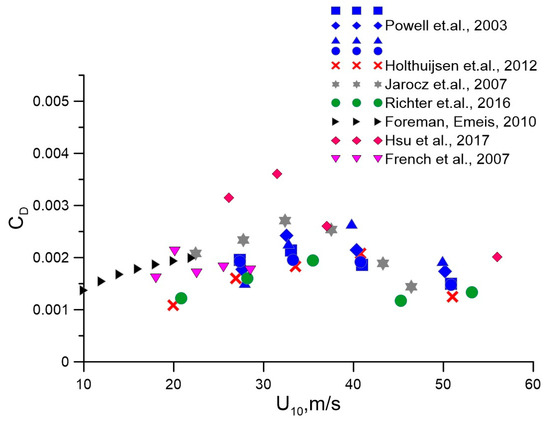
Figure 1.
Dependence of the neutral aerodynamic drag coefficient on . The symbols correspond to the field measurements from [28,31,32,33,34,35,36].
The main goal of the current study is concerned with the algorithm development for independent retrieval of the aerodynamic drag coefficient and turbulent stress (or wind friction velocity) directly from cross-polarized Sentinel-1 IW-mode SAR images for a wide range of wind conditions, including hurricanes. Empirical dependences of the scattered signal parameters on the atmospheric boundary layer characteristics mentioned above were obtained by comparing the values of the radar normalized cross section from SAR-images with measurements from stepped frequency microwave radiometer (SFMR) data. We use these measurements to obtain the values of the friction velocity, aerodynamic drag, and wind speed obtained with the empirical dependencies of ocean surface emissivity on wind parameters proposed in [24], in the framework of the alternative approach using collocated GPS-dropsondes and SFMR data.
The paper is organized as follows. In Section 2 we introduce the methodology and instruments used for wind measurements and define the analyzed dataset including each TCs category and its name, plus the time and date of SAR and SFMR data acquisition, together with its spatio-temporal collocation details. In Section 3 we describe an approach for the atmospheric boundary layer parameters retrieval from the SFMR data. In Section 4 we obtain the dependencies of the Sentinel-1 NRCS for VH-polarization on the 10-m wind speed, friction velocity and aerodynamic drag coefficient as retrieved from the collocated SFMR data using the approach from [24] and compare the wind speed obtained using the proposed dependencies with existing models (S1IW.NR [17], MS1A [15], H14S, H14E [16], S-C2PO [39]). The conclusions are provided in Section 5.
2. Methodology, Instruments and Datasets
To develop a method for determining the drag coefficient, turbulent stress (or associated friction velocity), and wind speed from remote sensing data, an array of SAR images of tropical cyclones in the Atlantic basin has been considered. C-band SAR acquisitions (with a frequency of 5.405 GHz) were performed in dual polarization (VV+VH, HH+HV) from the European Space Agency (ESA) Sentinel-1 mission. Sentinel-1 operates in four acquisition modes—Stripmap (SM), Interferometric Wide swath (IW), Extra-Wide swath (EW) and Wave (WV). In the present study the IW mode was used for the analysis, and its swath has a width of 250 km and captures 3 sub swaths. The spatial gridding of the IW mode is 5 × 20 m. Data was acquired for incidence angles in the range 30.85°–45.57°. All of the products used in the present study were obtained at SAR Level-1 GRD from the ESA Copernicus Open Access Hub (https://scihub.copernicus.eu/ (accessed on 24 November 2021)) for 6 hurricane scenes listed in Table 1. We applied the Sentinel Application Platform 8.0 (SNAP) to the SAR images in order to calibrate them and to perform thermal noise (NESZ) removal. An example of a SAR image for one of the selected hurricanes, its track and mean wind speed (MWS) distribution along the track is illustrated in Figure 2.

Table 1.
List of selected TCs, Sentinel-1 and SFMR acquisition time.
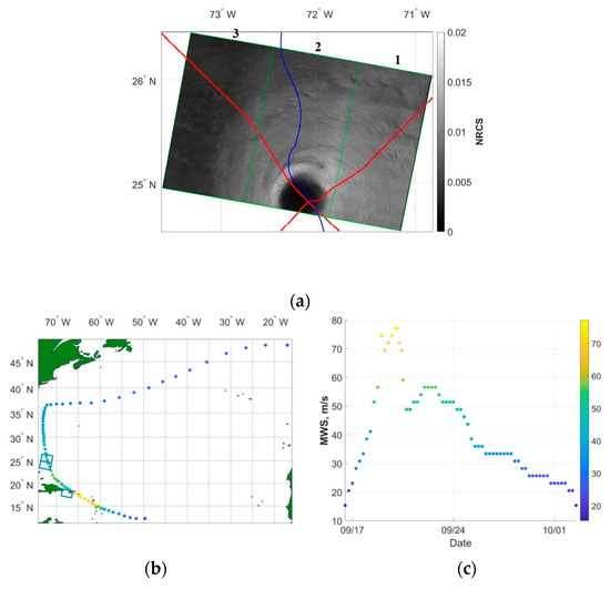
Figure 2.
Dataset illustration for Hurricane Maria 23 September 2017: (a) SAR image for IW mode and VH polarization, red curve—the track of the aircraft carrying SFMR superimposed on the Sentinel-1 image, blue curve—hurricane track; (b) Hurricane Maria track with the maximum wind speed indicated with color and selected for the analysis of the SAR image contours; (c) the distribution of maximum wind speed values of Hurricane Maria in time (data from https://www.nhc.noaa.gov/data/#hurdat (accessed on 1 December 2021)).
VH NRCS datasets from the Sentinel-1 Interferometric Wide swath SAR images with the extracted noise-equivalent sigma-zero (NESZ) data were combined with the collocated ocean surface emissivity from the NOAA/Hurricane Research Division’s Stepped-Frequency Microwave Radiometer (SFMR)—an airborne instrument measuring the microwave radiation from the ocean surface. The main value that the radiometer measures at C-band frequencies 4.55, 5.06, 5.64, 6.34, 6.96 and 7.22 GHz is the brightness temperature of the ocean, which can be recalculated into ocean surface emissivity. The data measured by SFMR is used in the wind speed retrieval algorithm, based on the geophysical model function (GMF) relating surface emissivity Ew and wind speed [40]. It provides values of surface wind speed and rain rate within TCs in real time. The spatial resolution of the SFMR measurements is 1.5 km for a typical aircraft speed of 150 m/s, with the duration of data acquisition for all SFMR channels of 10 s. The acquisition time of SFMR data for the TCs is listed in Table 1. In the present study, instead of the generally accepted GMF, we use our alternative geophysical model function relating CD (Ew), (Ew) and (Ew) as proposed in [24]. Its brief description is given in Section 3.
Ocean surface emissivity recalculated further into atmospheric parameters from SFMR data was averaged inside segments along the flight track with a step of 2 km, while the collocated SAR image data were averaged inside a square with a side of 2 km centered at the middle of the corresponding 2-km segment.
Along with the dependencies of NRCS on aerodynamic drag and friction velocity, the dependence of NRCS on wind speed was also considered in order to make a comparison with the previously constructed GMFs to make sure that the proposed approach is valid. The results of retrieval were validated using SMAP radiometric measurements. The NASA SMAP spacecraft carries an L-band radiometer instrument having a large, 1000 km swath width in a near-polar orbit. The SMAP L-band radiometer measures the microwave emission (brightness temperature), which can be co-located with Sentinel-1 images, with time differences of 3 h. SMAP data have a spatial resolution of 0.25° × 0.25°. In the present study the Level-3 (L3) soil moisture product is used, providing the surface wind speed data with 36 km × 36 km spatial resolution for the validation of wind speeds obtained from the Sentinel-1 images.
3. Geophysical Model Function for the SFMR Data
NOAA GPS-dropsondes are widely used instruments for measuring wind speed at a height of 10 m in tropical cyclones. In most cases a surface-adjusted wind speed is used because of technical difficulties that arise during measurements at the surface as a result of extreme weather conditions. One of the approaches for estimating such wind speeds within the 150-m atmospheric layer was used in [40]. This approach is based on the calculation of the wind speed averaged inside the lower atmosphere at a height of 150 m, while the wind speed at a height of 10 m is recalculated by multiplying the obtained averaged value by 0.85. In [41], an evaluation of the WL150 algorithm was made with respect to the SFMR winds. It demonstrated that wind averaging over thinner layers, specifically 100 m, 50 m, and especially the 25 m layer, have lower biases and are more appropriate for the retrieval of 10 m winds. It was thus concluded that winds obtained with the WL150 algorithm recalculated into 10-m surface wind are characterized by noise and biases. It was also emphasized in [41] that direct velocity measurements from GPS-dropsondes are obtained from the analysis of data using positions, which, in turn, are determined by measurements from GPS chips, information on the operation of which is currently insufficient. Therefore, the methods used for GPS-dropsonde 10-m wind speed retrieval require further investigation.
In the previous studies we proposed an approach to determine the wind speed at a 10 m height, as well as the friction velocity and aerodynamic drag coefficient, excluding the use of the WL150 algorithm or direct measurements of 10-m winds from GPS-dropsondes [24]. The measurements from SFMR were calibrated using the collocated GPS-dropsonde measurements for TC conditions. Twenty Category 4 and 5 TCs for the hurricane seasons 2001–2017 in the Atlantic basin were considered. The first step was the retrieval of the marine atmospheric boundary layer dynamic parameters from the GPS-dropsonde measurements. A generally accepted approach that is usually applied in technical hydrodynamics for turbulent boundary layers observed in aerodynamic pipes was considered. In the framework of this approach, airflow velocity profiles averaged over turbulent fluctuations are used to obtain the wind parameters. Velocity profiles are assumed to be self-similar and consist of a logarithmic part and a “wake” part, characterized by the airflow adaptation to the undisturbed part [24,42]. The retrieval of the 10 m wind speed, friction wind speed, and aerodynamic drag coefficient is performed from the wake part. This approach provides the opportunity to avoid the use of the logarithmic part of the boundary layer located closer to the water surface where the data are characterized by large scatter and errors, and neutralize the effect of profile deformation due to the wave-induced flux. To apply the self-similar laws, a statistical averaging of the GPS-dropsondes velocity profiles was applied. In order to do this for each individual TC, groups were constructed from a number of wind profiles selected at approximately the same distance from the center of each TC over the period of one day. The profiles demonstrating similar qualitative and quantitative behavior were combined into 3 conditional datasets: corresponding to the eye of the hurricane, to the region near the wall of the TC (10 m wind speeds were above 15 m/s), and to the outer region (10 m wind speeds were less than 15 m/s). For the further analysis we used only the wind profiles averaged over the profile groups corresponding to the region near the wall of the TC.
To develop an approach for the retrieval of the boundary layer parameters from the wake part of the self-similar velocity profiles, an approximation of self-similar velocity profiles observed in a wind channel or above a flat plate was used [24,43]:
here, is the maximum velocity in the turbulent boundary layer, is the friction velocity, is the boundary layer thickness, κ = 0.4 is the von Karman constant, and and are constants. The second-degree polynomial approximation of the “wake” part, i.e., for was used to obtain the values of (see [24]):
Comparing the expression (2) with (1) gives (see [24]):
The constants and were obtained through the approximation of experimental data (see [24]) using expressions (1): and . Then, using (4), the friction velocity can be calculated, and using the obtained values of the roughness parameter, the 10 m wind speed, and the aerodynamic drag coefficient can be calculated (see [24]):
here = 10 m.
The obtained within this algorithm is different from the surface wind speed determined with the WL150 algorithm [40]. and can be related with the following expression = 1.02 − 2.22, and it is obvious that and are highly correlated, as the calculated correlation has a value of 0.97. This relation is fitted to the data in the range of 15–57 m/s and does not apply equally well over this range; in particular, the scatter of wind speed values at the lower boundary of the proposed range gives a 13% discrepancy for the and , and for the upper boundary its value is 1.8%.
The next step of the investigation reported in [24] was the construction of a method for retrieval of the atmospheric boundary layer parameters from the ocean surface emissivity data due to the collocation of the GPS-dropsondes and the SFMR. The value of SFMR emissivity corresponding to the GPS-dropsonde coordinates was obtained and averaged over the chosen GPS-dropsonde groups. , , and were calculated from GPS-dropsonde data using the method proposed above and compared to the obtained values. In the present study, we have made a refinement of the retrieved atmospheric boundary layer parameters in comparison with the results presented in [24] using an additional verification of the friction velocity value using the constant flow part of the atmospheric boundary layer. The updated dataset is illustrated by the small symbols in Figure 3a–c. To construct the dependences of the averaged values of , , and , on the mean , the data illustrated by the small symbols was averaged inside bins (see large symbols in Figure 3a–c); the number of bins was equal to 10 and was chosen to meet the condition that the bins should contain a sufficient number of points for averaging—approximately 10. The obtained dependencies have the following form:
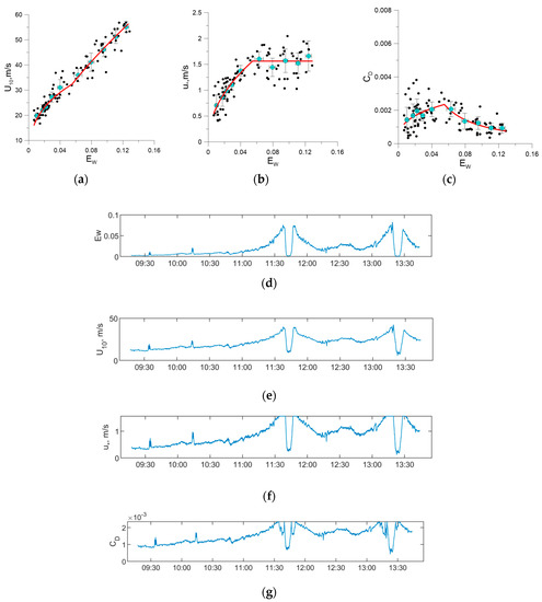
Figure 3.
The dependencies of surface wind speed (a), the wind friction velocity (b), and drag coefficient of the ocean surface (c), from GPS-dropsondes data on the ocean surface emissivity. The small symbols are the results of calculations for individual statistical ensembles composed of velocity profiles measured under approximately the same conditions; the large cyan symbols are mean values obtained from averaging inside the Ew bins, approximations (6)–(8) of the averaged data illustrated by the large symbols are shown in red color. The solid black line corresponds to the GMF from [40]. Time dependencies of ocean surface emissivity Ew (d), wind speed (e), friction velocity (f) and the aerodynamic drag coefficient CD (g) for Hurricane Maria from 23 September 2017.
The dependencies on the ocean surface emissivity of the surface wind speed, wind friction velocity, and aerodynamic drag coefficient of the ocean surface obtained from the GPS-dropsondes using the algorithm described above are illustrated in Figure 3a–c. It can be seen that the proposed algorithm is valid for the wind friction velocity retrieval only for wind speeds not exceeding 32 m/s due to the effect of saturation observed within the confidence intervals. It should be mentioned that the obtained saturation effect needs to be further verified with a larger amount of data, so a weak dependence of friction velocity on the emissivity cannot be excluded. The illustrated time dependencies of ocean surface emissivity , and CD for Hurricane Maria are presented in Figure 3d–g. It can be seen that the values of Ew and correspondingly the values of and are greatly reduced in the region of the hurricane eye, while at the same time the drag coefficient reduces sharply at the hurricane wall where the largest wind velocity values are observed.
It should be mentioned that despite the fact that the dataset used to obtain the dependencies (2)–(4) included measurements inside Category 4 and 5 hurricanes, at a significant distance from the analyzed hurricanes centers, low and moderate wind speeds were also observed (the lower limit of the analyzed velocities was 15 m/s), which are typical for hurricanes of lower categories. In this regard, the proposed algorithm may also be used to estimate the parameters in hurricanes of lower categories.
Below we use the dependencies (6)–(8) to obtain the values for the atmospheric boundary layer dynamic parameters. On the basis of a comparison of these values with the SAR data, we construct the model for the retrieval of atmospheric boundary layer dynamic parameters (, CD and —the last one is used as an auxiliary dependence) from Sentinel-1 IW mode cross-pol images, which we will refer to as MADP-S1. A flowchart diagram showing all analysis steps and their connections is shown in Figure 4.
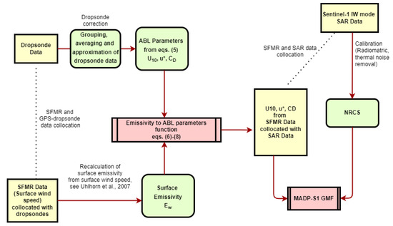
Figure 4.
Flowchart diagram showing all analysis steps and their connections made to obtain the MADP-S1 GMF.
4. Retrieval of Atmospheric Boundary Layer Dynamic Parameters at Strong Winds from Sentinel-1 SAR-Images
As a first step we obtained the dependence of NRCS on wind speed . This relationship was proposed for angles in the range of 30.85°–45.57° and for wind speeds in the range of 15–69 m/s. The construction of the dependence of NRCS on wind speed was conditioned by the need for comparison with the previous GMFs in order to confirm the validity of the approach for and CD retrieval proposed here.
4.1. Wind Speed Retrieval
For the construction of the dependency of NRCS on the wind speed , an approach proposed in [16] was used. This approach is based on the piecewise power law function applied to the number of selected wind speed regions. In this case, the angular dependence of NRCS in every i-th wind speed interval is achieved, since the proposed approximation coefficients depend on the incidence angle θ. We have used similar power dependence; however, to ensure the continuity of the approximation, a vertical shift was additionally used:
Thus, in order to construct a piecewise approximation, we carried out the following procedure:
Step 1: the dataset is divided into three groups according to the three sub swaths,
Step 2: we chose a sub swath for the analysis and set the lower boundary of the first approximation interval of wind velocity to 15 m/s in accordance with the limit of the capabilities of our algorithm for data retrieval using SFMR, as described in Section 3,
Step 3: the default i-th approximation interval of wind velocity was chosen to be 5 m/s; within this interval the approximation of the NRCS data was performed using the power dependence , and then the upper boundary of the chosen wind velocity interval was iteratively increased by 1 m/s and the approximation was made again. This procedure was repeated until the exponent of the power approximation within the selected interval did not change by more than 10 percent,
Step 4: in the case of a change in the power approximation exponent by more than 10 percent, we set the upper boundary of the i-th wind velocity interval (Ubi(θ)) and the values of the coefficients and ,
Step 5: the value of Ubi(θ) then becomes the new lower boundary of the (i + 1)-th approximation interval, after which we returned to step 3 to approximate data within the (i + 1)-th interval. The procedure was repeated until the upper limit of the data array was reached,
Step 6: the approximations obtained in steps 3–5 inside each wind speed interval thus formed a piecewise GMF. The continuity of the constructed GMF was ensured by vertically shifting each individual approximation by the value .
The approximations were made inside each of the three sub swaths covering the incidence angles 30.85°–35.9° (sub swath 1), 35.9°–41.3° (sub swath 2) and 41.3°–45.57° (sub swath 3). The resulting values of , , , and Ubi(θ) are listed in Table 2.
Table 2.
The MADP-S1 power approximation coefficients used for the wind velocity retrieval.
Figure 5 shows the dependencies of the NRCS for the three incidence angle bins corresponding to the three sub swaths outlined above. The proposed GMF is compared to the previously reported GMFs referred to as MS1A, S1IW.NR, H14E, H14S and S-C2PO. It can be seen that in the high-to-severe wind speed region ( > 30 m/s), the proposed MADP-S1 GMF significantly underestimates the wind speed compared to H14S, while for moderate winds MADP-S1 overestimates wind speeds compared to S-C2PO. The MADP-S1 is close to H14E and MS1A for sub swaths 1 and 2, while for sub swath 3 it demonstrates an underestimation for > 35 m/s compared to MS1A and an overestimation compared to H14E. It may be concerned with the fact that for the first and second sub swaths the datasets have good coverage of (up to 50–60 m/s), but for the third sub swath this data set covers only the region of wind speeds less than 35 m/s. Obviously, this is because the selected SAR images did not contain areas with strong winds in the third sub swath corresponding, in particular, to the wall of the hurricane.
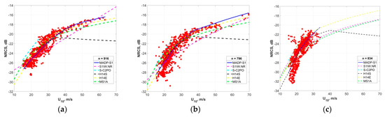
Figure 5.
The dependencies of NRCS on wind speed for sub swath 1 (a); sub swath 2 (b); and sub swath 3 (c). The blue solid line corresponds to the MADP-S, and the dotted curves illustrate recently created GMFs: S1IW.NR (purple), MS1A (green), H14E (yellow), H14S (black), and S-C2PO (light blue); n corresponds to the number of data points used to construct the proposed GMF.
Figure 6 shows the validation of retrievals made with the MADP-S1, H14E, MS1A, and S1IW.NR using wind speeds measured by SMAP for the dataset from Table 3. In general, the mean difference (bias), which is calculated as the difference between the modeled and measured values of wind velocity, is negative for MADP-S1 and H14E, which is opposite to the biases calculated for MS1A and S1IW.NR; this indicates the underestimation of the modeled values. It can be seen that this underestimation predominantly appears in the region of moderate-to-strong winds and can be corrected in the future if the data array is expanded in the area of extremely high wind speeds. However, it should be noted that the modeled and measured wind speeds are well correlated. Analyzing Figure 6, it can be seen that the overall difference between the statistical parameters for MADP-S1 and H14E are quite small, except for the bias, which has a larger value for H14E. This is apparently because in the case of data modeled using MADP-S1, the data considered in the region of low-to-moderate wind speeds turn out to be somewhat overestimated and, on the contrary, underestimated in the region of high wind speeds, while for the H14E there is only an underestimation of the simulated values with respect to the measured ones. On the contrary, the values calculated using MS1A turn out to be overestimated in the region of extreme winds in relation to those measured using SMAP; in addition, they demonstrate a rather large scatter in the region of extreme wind speeds. An overestimation for extreme winds is also demonstrated by S1IW.NR; however, the scatter of data for this turns out to be smaller than for MS1A. Analyzing the obtained results, one can come to the conclusion that MADP-S1 and H14E simulated values demonstrate the same trend with wind speed, different from S1W.NR. It should be noted, however, that in the case of the validation of retrievals made with the H14E and S1IW.NR using wind speeds measured by SFMR from the dataset from Table 1, the situation changes to the opposite and H14E shows a linear trend, in contrast to S1IW.NR (see Figure 6e,f). Perhaps this discrepancy is due to different instruments for data acquisition used to create these GMFs. The question of the influence of data source choice for the construction of the GMF on the results of its subsequent validation requires a more detailed study in the future. It should also be mentioned that the main weakness of the validation using the SMAP tool is due to the large SMAP footprint size (36 × 36 km), so it is difficult to capture the extreme winds because they fill only a modest fraction of the footprint. As a result, the maximum value of wind speeds measured using SMAP will be lower than the maximum value of the wind speeds measured using SFMR and used while constructing the proposed GMF.

Figure 6.
The dependencies of wind speed for all sub swaths on the wind speed retrieved from the SMAP measurements: MADP-S1 (a); H14E (b); MS1A (c); S1IW.NR (d). n corresponds to the number of data points. The dependencies of wind speed for all sub swaths on the wind speed retrieved from the SFMR measurements (on the basis of the dataset from Table 1): H14E (e); S1IW.NR (f).
Table 3.
List of TCs selected for validation, Sentinel-1 and SMAP acquisition time.
4.2. Wind Friction Velocity Retreival
For construction of the dependency of the NRCS on the friction velocity, we use power dependence with a vertical shift similar to (9):
The values of coefficients used in (9) are presented in Table 4. The boundary values of the friction wind speed regions containing different powers are referred to as .
Table 4.
The MADP-S1 power approximation coefficients for the friction velocity retrieval.
Figure 7 illustrates the dataset for the NRCS versus the friction velocity values obtained using expression (7). The dataset is limited with a cutoff value for equal to 1.56, which corresponds to the NRCS value of −21.4 dB. This cutoff is obtained due to the saturation effect observed for the dependency of ocean emissivity Ew on the friction velocity for the values of Ew exceeding 0.055 (see expression (7)).
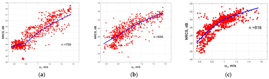
Figure 7.
Dependencies of the NRCS on the friction velocity for sub swath 1 (a); sub swath 2 (b); and sub swath 3 (c). The blue curve represents the power approximation from Table 3. n corresponds to the number of data points used to construct the proposed GMF.
4.3. Aerodynamic Drag Coefficient Retreival
The dependency of the NRCS on the aerodynamic drag coefficient was determined in a similar manner to (9) and (10) (see Table 5 and Table 6). The main difference was that the approximation parameters were obtained without taking into account the sub swath dependence, due to the lack of data for the drag coefficient. It can be seen from Figure 8 that there are two branches of the NRCS on CD dependence corresponding to different parts of the piecewise dependency of the aerodynamic drag coefficient on the emissivity Ew (see Figure 3c). The value of CD at which these dependencies intersect equals 0.00232, which corresponds to the NRCS value −21.4 dB (see Figure 8). Despite the fact that the dependence of NRCS on the aerodynamic drag coefficient is ambiguous, the CD retrieval can be performed precisely, and in accordance with the proposed dependencies, there may be cases when different NRCS correspond to the same values of the drag coefficient.
Table 5.
The MADP-S1 power approximation coefficients for the aerodynamic drag coefficient retrieval (NRCS with values greater than 0.0079 (−21.4 dB)).
Table 6.
The MADP-S1 power approximation coefficients for the aerodynamic drag coefficient retrieval (NRCS with the values less than 0.0079 (−21.4 dB)).
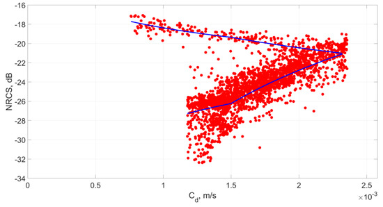
Figure 8.
Dependencies of the NRCS on the drag coefficient for all sub swaths; the blue curve represents the proposed approximations. The number of points is equal to 269 (for the upper dependence) and 2235 (for the lower dependence).
It should be mentioned that a validation of the GMF should include the comparison of the modeled values with the measurements. However, there are currently no reliable data on wind friction velocity and drag coefficient, especially corresponding to extreme wind speeds, as all the current datasets demonstrate a large scatter (see [44]). To validate the results of CD modeling with our GMF, we used the approximations of the datasets presented in [31,32,33,35,36]. On this basis, we have built a dependence of modeled drag coefficient on CD obtained with these approximations using SMAP retrieved wind speeds (see Figure 9b). It can be seen from Figure 9b that different datasets demonstrate different behavior (some of them overestimate the drag coefficient and some of them underestimate it), which again is due to the fact that in the area of extremely high winds there is a large scatter in the datasets, and a significant uncertainty in the functional dependencies of CD on .
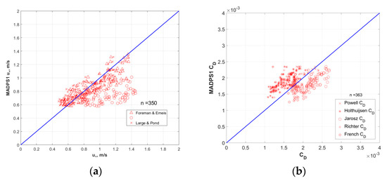
Figure 9.
The friction velocity modeled with MADP-S1 versus the values obtained from the bulk-formulas from ([27,28]; here Foreman & Emeis 1 corresponds to , and Foreman & Emeis 2 corresponds to , see [28])) using SMAP retrieved wind speeds (a). The dependency of drag coefficient modeled with MADP-S1 versus the values of drag coefficient obtained from the dataset parameterization on from [31,32,33,35,36] using SMAP-retrieved wind speeds (b).
To construct such dependencies for friction velocity in the range specified in our study, we used the parameterizations of friction velocity on from [27,28]. It can be seen from Figure 9a that different parameterizations give different results, which indicates an uncertainty in determining the value of friction velocity. It is obviously related to the choice of a specific parameterization, and thus the quality of the results greatly depends on which particular parameterization we choose from the currently existing ones.
The resulting dependences of NRCS on , and CD were used to retrieve the two-dimensional distribution of aerodynamic drag, friction velocity, and wind velocity from the SAR image of a tropical cyclone. Figure 10 contains the results of , and CD retrieval from the SAR image for Hurricane Maria on 23 September 2017 using the proposed MADP-S1 GMF. Since MADP-S1 works across a wide range of wind speeds, it allows the retrieval of all the wind speeds in the image up to the highest values observed in the wall area. Since the proposed GMF has limitations for the case of very low wind speeds (less than 15 m/s) particularly observed in the region of the hurricane eye, such wind speeds can be retrieved on the basis of generally accepted GMFs, such as CMOD5, in a similar way as was proposed in [15]. It is seen from Figure 10b that the distribution of the friction velocity demonstrates an increase in the area of the hurricane wall, until, at some distance from the center of the hurricane, it finally reaches its cutoff value of 1.56, and then in a region far from the hurricane eye it gradually decreases with distance from the hurricane center. It should be mentioned that for the illustration of friction velocity as demonstrated in Figure 10b,c, we use the cutoff value everywhere inside the area where the NRCS becomes more than −21.4 dB (for the friction velocity) corresponding to the cutoff values specified in Figure 7. At the same time, the drag coefficient shows an increase in the region of the wall of the eye, and then a noticeable decrease. When moving away from the wall of the eye, the drag coefficient increases again and reaches its maximum value of 0.00232. In the outer regions of the hurricane, the drag coefficient decreases monotonically (see Figure 10c). The effect of the drag coefficient decrease for extreme wind speeds was discussed in [36,38], and may be associated with a number of factors, such as the effects of form drag [45,46], separation [29], sheltering [47], sea spray [48,49,50], and foam [32,51,52] on the wind-wave momentum exchange, observed at extremely high wind speeds.
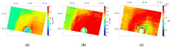
Figure 10.
Illustration of the distributions of (a), (b) and CD (c) retrieved from the Hurricane Maria SAR image of 23 September 2017.
5. Conclusions
Improving the accuracy of tangential turbulent stress and exchange coefficients retrieval which determine the large-scale ocean circulation is crucial in forecasting the development of tropical cyclones. Despite the fact that conventional C-band geophysical model functions are normally used for wind speed retrieval, the small-scale surface roughness determining the value of microwave backscatter is related to the tangential turbulent stress τ, which means that the dependence of NRCS on τ must be stronger than the dependence of NRCS on wind speed. The values of tangential turbulent stress (or associated friction velocity) are usually obtained with bulk-formulas that have limitations concerned with the significant uncertainties in determining the drag coefficient for strong winds. In the present study we have made an attempt to construct a MADP-S1 GMF that makes it possible to obtain the values of and CD from Sentinel-1 IW cross-polarized SAR images.
The first step in constructing MADP-S1 was concerned with the establishment of average interdependencies relating ocean emissivity from SFMR and the values of , and CD, similar to [24]. This approach allows one to determine these three parameters from one retrieval. The next step was the collocation of SAR images with SFMR data. The final step was the comparison of the NRCS with the values of and CD calculated using the developed radiometric relations. The interval for friction velocities for MADP-S1 retrieval ranges from 0.55–1.56 m/s and the aerodynamic drag coefficient values lie in the range of 0.00076–0.00232. We also obtained the dependence of the NRCS on the wind speed in order to compare it with previous similar dependences (MS1A, S1IW.NR, H14E, H14S and S-C2PO models) to show that the proposed approach is valid. It was shown that MADP-S1 GMF is consistent with H14E and MS1A.
It should be mentioned that as the parametrical relations between , and CD were used to construct the proposed GMF through the emissivity, these parameterizations are inherently included in the obtained dependencies of NRCS on these atmospheric boundary layer parameters. Therefore, some features of the proposed radiometric parameterizations are reflected in the results of calculations within the framework of the proposed GMF (such as, for example, the aerodynamic drag coefficient reduction).
As an example, on the basis of the proposed MADP-S1 GMF, the wind speed, wind friction velocity, and aerodynamic drag coefficient fields using the Hurricane Maria 23 September 2017 SAR image were retrieved; the results were presented in the form of two-dimensional images. For the wall of the eye, a sharp increase in the wind speed and a decrease in the drag coefficient were observed.
We should note that the strength of the proposed GMF is concerned with the possibility of wind speed, drag coefficient and friction velocity retrieval from cross-polarized Sentinel-1 IW SAR images at extremely high wind speeds (up to 69 m/s depending on the image sub swath). At the same time, the weakness of the proposed GMF includes the low upper limit for wind speed retrieval in the third subswath (only 35 m/s), as well as the fact that the GMF for the drag coefficient retrieval does not contain an angular dependence. These weaknesses can be eliminated in the future by expanding the data array.
Author Contributions
Conceptualization, O.E., N.R., E.P. and Y.T.; methodology, Y.T., N.R., E.P., O.E. and D.S.; software, N.R. and E.P.; validation, E.P. and N.R.; investigation, N.R., E.P. and O.E.; data curation, N.R. and E.P.; writing—original draft preparation, O.E., N.R. and E.P.; writing—review and editing, O.E., N.R. and E.P.; visualization, N.R. and E.P.; supervision, Y.T. and O.E. All authors have read and agreed to the published version of the manuscript.
Funding
This work was carried out under the financial support of the Russian Science Foundation Project No 21-17-00214.
Data Availability Statement
The data presented in this study are available on request from the corresponding author.
Conflicts of Interest
The authors declare that they have no conflict of interest.
References
- Horstmann, J.; Thompson, D.R.; Monaldo, F.; Iris, S.; Graber, H.C. Can synthetic aperture radars be used to estimate hurricane force winds? Geophys. Res. Lett. 2005, 32, L22801. [Google Scholar] [CrossRef]
- Shen, H.; Perrie, W.; He, Y. A new hurricane wind retrieval algorithm for SAR images. Geophys. Res. Lett. 2006, 33, L21812. [Google Scholar] [CrossRef]
- Yueh, S.; Stiles, B.W.; Liu, W.T. QuikSCAT wind retrievals for tropical cyclones. IEEE Trans. Geosci. Remote Sens. 2003, 41, 2616–2628. [Google Scholar] [CrossRef]
- Williams, B.A.; Long, D.G. Estimation of hurricane winds from SeaWinds at ultrahigh resolution. IEEE Trans. Geosci. Remote Sens. 2008, 46, 2924–2935. [Google Scholar]
- Stiles, B.W.; Dunbar, R.S. A neural network technique for improving the accuracy of scatterometer winds in rainy conditions. IEEE Trans. Geosci. Remote Sens. 2010, 48, 3114–3122. [Google Scholar] [CrossRef]
- Fernandez, D.; Carswell, J.R.; Frasier, S.; Chang, P.S.; Black, P.G.; Marks, F.D. Dual-polarized C- and Ku-band ocean backscatter response to hurricane-force winds. J. Geophys. Res. 2006, 111, C08013. [Google Scholar]
- Weissman, D.E.; Bourassa, M.A. The influence of rainfall on scatterometer backscatter within tropical cyclone environments—Implications on parameterization of sea-surface stress. IEEE Trans. Geosci. Remote Sens. 2011, 49, 4805–4814. [Google Scholar] [CrossRef]
- Stoffelen, A.; Anderson, D. Scatterometer data interpretation: Estimation and validation of the transfer function CMOD4. J.Geophys. Res. Ocean. 1997, 102, 5767–5780. [Google Scholar] [CrossRef]
- Quilfen, Y.; Chapron, B.; Elfouhaily, T. Observation of tropical cyclones by high-resolution scatterometry. J. Geophys. Res. Ocean. 1998, 103, 7767–7786. [Google Scholar] [CrossRef]
- Hersbach, H. CMOD5, an improved geophysical model functionfor ERS C-band scatterometry, technical memo; European Center for Medium-Range Weather Forecasts: Reading, UK, 2003. [Google Scholar]
- Hersbach, H. Comparison of C-Band Scatterometer CMOD5.N Equivalent Neutral Winds with ECMWF. J. Atmos. Ocean. Technol. 2010, 27, 721–736. [Google Scholar] [CrossRef]
- Stoffelen, A.; Verspeek, J.A.; Vogelzang, J.; Verhoef, A. The CMOD7 Geophysical Model Function for ASCAT and ERS Wind Retrievals. IEEE J. Sel. Top. Appl. Earth Obs. Remote Sens. 2017, 10, 2123–2134. [Google Scholar] [CrossRef]
- Vachon, P.W.; Wolfe, J. C-band cross-polarization wind speed retrieval. IEEE Geosci. Remote Sens. Lett. 2011, 8, 456–459. [Google Scholar] [CrossRef]
- Zhang, B.; Perrie, W.; He, Y. Wind speed retrieval from RADARSAT-2 quad-polarization images using a new polarization ratio model. J. Geophys. Res. 2011, 116, C08008. [Google Scholar]
- Mouche, A.; Chapron, B.; Zhang, B.; Husson, R. Combined Co- and Cross-Polarized SAR Measurements Under Extreme Wind Conditions. IEEE Trans. Geosci. Remote Sens. 2017, 55, 6746–6755. [Google Scholar]
- Hwang, P.A.; Stoffelen, A.; van Zadelhoff, G.-J.; Perrie, W.; Zhang, B.; Li, H.; Shen, H. Crosspolarization geophysical model function for C-band radar backscattering from the ocean surface and wind speed retrieval. J. Geophys. Res. Ocean. 2015, 120, 893–909. [Google Scholar] [CrossRef]
- Gao, Y.; Sun, J.; Zhang, J.; Guan, C. Extreme Wind Speeds Retrieval Using Sentinel-1 IW Mode SAR Data. Remote Sens. 2021, 13, 1867. [Google Scholar] [CrossRef]
- Jones, W.L.; Schroeder, L.C. Radar Backscatter from the Ocean: Dependence on Surface Friction Velocity. Boundary-Layer Meteorol. 1978, 13, 133–149. [Google Scholar] [CrossRef]
- Weissman, D.E.; Davidson, K.L.; Brown, R.A.; Friehe, C.A.; Li, F. The relationship between the microwave radar cross section and both wind speed and stress: Model function studies using frontal air-sea interaction experiment Data. J. Geophys. Res. 1994, 99, C10087–C10108. [Google Scholar] [CrossRef]
- Liu, W.T.; Xie, X. Sea surface wind/stress vector. In Encyclopedia of Remote Sensing; Springer: New York, NY, USA, 2014; pp. 759–767. [Google Scholar] [CrossRef]
- Liu, W.T.; Tang, W. Relating wind and stress under tropical cyclones with scatterometer. J. Atm. Ocean Tech. 2016, 33, 1151–1158. [Google Scholar] [CrossRef]
- Troitskaya, Y.; Abramov, V.; Baidakov, G.; Ermakova, O.; Zuikova, E.; Sergeev, D.; Ermoshkin, A.; Kazakov, V.; Kandaurov, A.; Rusakov, N.; et al. Cross-Polarization GMF For High Wind Speed and Surface Stress Retrieval. J. Geophys. Res. 2018, 123, 5842–5855. [Google Scholar] [CrossRef]
- Ermakova, O.; Sergeev, D.; Rusakov, N.; Poplavsky, E.; Balandina, G.; Troitskaya, Y. Toward the GMF for Wind Speed and Surface Stress Retrieval in Hurricanes Based on the Collocated GPS-Dropsonde and Remote Sensing Data. IEEE J. Sel. Top. Appl. Earth Obs. Remote Sens. 2020, 13, 1–7. [Google Scholar] [CrossRef]
- Poplavsky, E.; Rusakov, N.; Ermakova, O.; Sergeev, D.; Troitskaya, Y. Towards an Algorithm for Retrieval of the Parameters of the Marine Atmospheric Boundary Layer at High Wind Speeds Using Collocated Aircraft and Satellite Remote Sensing. J. Mar. Sci. Eng. 2022, 10, 1136. [Google Scholar] [CrossRef]
- Edson, J.B.; Jampana, V.; Weller, R.; Bigorre, S.; Plueddemann, A.J.; Fairall, C. On the exchange of momentum over the open ocean. J. Phys. Oceanogr. 2013, 43, 1589–1610. [Google Scholar] [CrossRef]
- Fairall, C.W.; Bradley, E.F.; Hare, J.E.; Grachev, A.A.; Edson, J.B. Bulk parameterization of air-sea fluxes: Updates and verification for the COARE algorithm. J. Clim. 2003, 16, 571–591. [Google Scholar] [CrossRef]
- Large, W.G.; Pond, P. Open ocean momentum flux measurements in moderate to strong winds. J. Phys. Oceanogr. 1981, 11, 324–336. [Google Scholar] [CrossRef]
- Foreman, R.J.; Emeis, S. Revisiting the Definition of the Drag Coefficient in the Marine Atmospheric Boundary Layer. J. Phys. Oceanogr. 2010, 40, 2325–2332. [Google Scholar] [CrossRef]
- Donelan, M.A.; Haus, B.K.; Reul, N.; Plant, W.J.; Stiassnie, M.; Graber, H.C.; Brown, O.B.; Saltzman, E.S. On the limiting aerodynamic roughness of the ocean in very strong winds. Geophys. Res. Lett. 2004, 31, L18306. [Google Scholar] [CrossRef]
- Andreas, E.L.; Mahrt, L.; Vickers, D. A new drag relation for aerodynamically rough flow over the ocean. J. Atmos. Sci. 2012, 69, 2520–2537. [Google Scholar] [CrossRef]
- Powell, M.D.; Vickery, P.J.; Reinhold, T.A. Reduced drag coefficient for high wind speeds in tropical cyclones. Nature 2003, 422, 279–283. [Google Scholar] [CrossRef]
- Holthuijsen, L.H.; Powell, M.D.; Pietrzak, J.D. Wind and waves in extreme hurricanes. J. Geophys. Res. 2012, 117, C09003. [Google Scholar] [CrossRef]
- Jarosz, E.; Mitchell, D.A.; Wang, D.W.; Teague, W.J. Bottom-Up Determination of Air-Sea Momentum Exchange Under a Major Tropical Cyclone. Science 2007, 315, 1707–1709. [Google Scholar] [CrossRef] [PubMed]
- Hsu, J.Y.; Lien, R.C.; D’Asaro, E.A.; Sanford, T.B. Estimates of surface wind stress and drag coefficients in typhoon Megi. J. Phys. Oceanogr. 2017, 47, 545–565. [Google Scholar] [CrossRef]
- French, J.R.; Drennan, W.M.; Zhang, J.A.; Black, P.G. Turbulent fluxes in the hurricane boundary layer. Part I: Momentum flux. J. Atmos. Sci. 2007, 64, 1089–1102. [Google Scholar] [CrossRef]
- Richter, D.H.; Bohac, R.; Stern, D.P. An assessment of the flux profile method for determining air–sea momentum and enthalpy fluxes from dropsonde data in tropical cyclones. J. Atmos. Sci. 2016, 73, 2665–2682. [Google Scholar] [CrossRef]
- Takagaki, N.; Komori, S.; Suzuki, N.; Iwano, K.; Kurose, R. Mechanism of drag coefficient saturation at strong wind speeds. Geophys. Res. Lett. 2016, 43, 9829–9835. [Google Scholar] [CrossRef]
- Richter, D.H.; Wainwright, C.; Stern, D.P.; Bryan, G.H.; Chavas, D. Potential Low Bias in High-Wind Drag Coefficient Inferred from Dropsonde Data in Hurricanes. J. Atmos. Sci. 2021, 78, 2339–2352. [Google Scholar] [CrossRef]
- Zhang, K.; Huang, J.; Mansaray, L.R.; Guo, Q.; Wang, X. Developing a Subswath-Based Wind Speed Retrieval Model for Sentinel-1 VH-Polarized SAR Data Over the Ocean Surface. IEEE Trans. Geosci. Remote Sens. 2018, 57, 1561–1572. [Google Scholar] [CrossRef]
- Uhlhorn, E.W.; Black, P.G.; Franklin, J.L.; Goodberlet, M.; Carswell, J.; Goldstein, A.S. Hurricane Surface Measurements from an Operational Stepped Frequency Microwave Radiometer. Mon. Weather. Rev. 2007, 135, 3070–3085. [Google Scholar] [CrossRef]
- Polverari, F.; Sapp, J.W.; Portabella, M.; Stoffelen, A.; Jelenak, Z.; Chang, P.S. On dropsonde surface-adjusted winds and their use for the stepped frequency microwave radiometer wind speed calibration. IEEE Trans. Geosci. Remote Sens. 2022, 60, 1–8. [Google Scholar] [CrossRef]
- Kandaurov, A.A.; Troitskaya, Y.I.; Sergeev, D.A.; Vdovin, M.I.; Baidakov, G.A. Average velocity field in the air flow over the water surface in laboratory study of the hurricane conditions. Izv. Atmos. Ocean. Phys. 2014, 50, 399–410. [Google Scholar] [CrossRef]
- Hintze, J.O. Turbulence: An Introduction to Its Mechanism and Theory; McGraw-Hill: New York, NY, USA, 1959; p. 586. [Google Scholar]
- Chen, S.; Qiao, F.; Zhang, J.A.; Xue, Y.; Ma, H.; Chen, S. Observed drag coefficient asymmetry in a tropical cyclone. J. Geophys. Res. 2022, 127, e2021JC018360. [Google Scholar] [CrossRef]
- Makin, V.K.; Kudryavtsev, V.N.; Mastenbroek, C. Drag of the sea surface. Bound.-Layer Meteor. 1995, 73, 159–182. [Google Scholar] [CrossRef]
- Kukulka, T.; Hara, T.; Belcher, S.E. A model of the air-sea momentum flux and breaking wave distribution for strongly forced wind-waves. J. Phys. Oceanogr. 2007, 37, 1811–1828. [Google Scholar] [CrossRef]
- Troitskaya, Y.I.; Rybushkina, G.V. Quasi-linear model of interaction of surface waves with strong and hurricane winds. Izv. Acad. Sci. USSR Atmos. Oceanic Phys. 2008, 44, 621–645. [Google Scholar] [CrossRef]
- Andreas, E.L. Spray stress revisited. J. Phys. Oceanogr. 2004, 34, 1429–1440. [Google Scholar] [CrossRef]
- Kudryavtsev, V.N.; Makin, V.K. Impact of ocean spray on the dynamics of the marine atmospheric boundary layer. Bound.-Layer Meteor. 2011, 140, 383–410. [Google Scholar] [CrossRef]
- Troitskaya, Y.; Druzhinin, O.; Kozlov, D.; Zilitinkevich, S. “Bag-breakup” spume droplet generation mechanism at hurricane wind. Part II. Contribution to momentum and enthalpy transfer. J. Phys. Oceanogr. 2018, 48, 2189–2207. [Google Scholar] [CrossRef]
- Golbraikh, E.; Shtemler, Y.M. Foam input into the drag coefficient in hurricane conditions. Dynam. Atmos. Ocean 2016, 73, 1–9. [Google Scholar] [CrossRef]
- Troitskaya, Y.; Sergeev, D.; Kandaurov, A.; Vdovin, M.; Zilitinkevich, S. The Effect of Foam on Waves and the Aerodynamic Roughness of the Water Surface at High Winds. J. Phys. Oceanogr. 2019, 49, 959–981. [Google Scholar] [CrossRef]
Disclaimer/Publisher’s Note: The statements, opinions and data contained in all publications are solely those of the individual author(s) and contributor(s) and not of MDPI and/or the editor(s). MDPI and/or the editor(s) disclaim responsibility for any injury to people or property resulting from any ideas, methods, instructions or products referred to in the content. |
© 2023 by the authors. Licensee MDPI, Basel, Switzerland. This article is an open access article distributed under the terms and conditions of the Creative Commons Attribution (CC BY) license (https://creativecommons.org/licenses/by/4.0/).