On Surface Waves Generated by Extra-Tropical Cyclones—Part I: Multi-Satellite Measurements

Abstract

Surface waves generated by Extra-Tropical Cyclones (ETCs) can significantly affect shipping, fishing, offshore oil and gas production, and other marine activities. This paper presents the results of a satellite data-based investigation of wind waves generated by two North Atlantic ETCs. These ETCs were fast-moving systems, inhibiting resonance (synchronism) between the group velocity of the generated waves and the ETC translation velocity. In these cases, wave generation begins when the front boundary of the storm appears at a given ocean location point. Since developing waves are slow, they move backward relative to the storm, grow in time, and then leave the ETC stormy area through the rear sector. Multi-satellite observations confirm such a paradigm, revealing that the storm regions are filled with young developing wind waves, the most developed in the rear-right sector. As observed, the energy of these waves grew in time during the ETC life span. It is demonstrated that the extended-fetch concept (inherent for Tropical Cyclones) does not apply to ETC. Instead, by analogy, the concept of extended-duration wave growth is more relevant. Satellite observations confirmed the validity of duration-laws for waves generated by ETCs, and demonstrated that extended-fetch solutioncan be valid at time scales exceeding the lifespan of considered ETCs.

1. Introduction

In the North Atlantic, there are more than 10 extra-tropical cyclones (ETCs) every year with hurricane-force winds (e.g., [1]). ETCs and the ocean surface waves they generate can significantly affect shipping, fishing, offshore oil and gas production, and other marine activities. Estimating the probability of occurrence of high surface waves is one of the most important factors to consider in designing offshore and onshore infrastructures. Caused by these storm events, wave heights can become catastrophically high, with heights exceeding 20 m [1,2]. As argued in [3,4,5], the highest waves on Earth are generally found in the northeast Atlantic, making this region particularly interesting for investigation of extreme waves and conditions of their generation.

ETCs are a synoptic-scale atmospheric system in the mid-latitudes that have a basin-wide impact on the weather and climate of the North Atlantic. The North Atlantic Ocean is regularly traversed by ETCs and low-pressure winter systems originating in the Western part of the basin that can potentially generate dangerous extreme sea states [6,7,8]. The region where these extreme sea states occur is linked to the tracks of the low-pressure systems in the North Atlantic basin. The variability of these storm tracks presents a primary dipole pattern, with centers in the extreme northeastern Atlantic and west of Portugal. A strong north-eastward extension of the storm tracks causes strong maritime flow, giving rise to mild European winters [9]. Indeed, in the North Atlantic, very high waves are to be found in the storm track region of the basin [10,11], and the west coast of Europe is regularly exposed to huge swells generated by the North Atlantic cyclones that cross the basin from west to east, with significant socio-economic consequences and increased coastal vulnerability [12,13].

In the absence of in situ measurements, satellite observations are the most robust and reliable sources for monitoring and forecasting extreme wind/waves, taking advantage of their availability, regularity, bandwidth, and improved spatial resolution. At present, large multi-mission databases of surface wind and significant wave height (SWH) from altimetry are available to study ocean wind, wave properties, and climate [14]. Although satellite altimetry suffers from incomplete temporal and spatial coverage, the amount of available data from successive satellite passes enables the calculation of wind and SWH distributions and allows estimating climatological fields, trends, and extreme values prediction [3,15]. In addition to existing satellite capabilities for monitoring extreme events, the CFOSAT (Chinese-French Oceanographic Satellite) mission, launched in 2018, can now simultaneously provide the ocean surface wind field and 2D spectral wave distributions. CFOSAT does carry SCAT, a Ku-band wind field scatterometer, and a unique SWIM (Surface Wave Investigation and Monitoring) Real Aperture Scanning Radar System designed for directional detection of ocean surface waves [16,17].

Wave fields generated by moving atmospheric systems (tropical cyclones (TC), ETCs, and polar lows (PL)) have several unique features that make them very different from waves generated by stationary wind fields. In general, these features originate from the fact that wave generation permanently occurs under a moving wind field. As a result, developing waves in a moving storm with a given spatial scale of wind field (i.e., cyclone radius), stay under wind forcing for a longer time than in a stationary one and thus, become more developed (higher). When the evolving group velocity of the developing waves starts to match the translation velocity of the storm, the waves remain under the wind forcing for an “infinitely” long time. Resulting wave heights and wavelengths can thus take on anomalous values, significantly exceeding the expected values prescribed by the given wind speed and the size of the storm area. This phenomenon is called extended (effective) fetch or group velocity resonance. It is inherent for the waves generated by moving TC [18,19,20,21,22,23,24,25] and PL [26,27,28]. The importance of this mechanism for the waves generated by ETCs was argued in [29] and also found in numerical simulations using WAM [30] and WW3 [31] models. Satellite observations of SWHs generated by ETC over the global ocean also revealed a clear dependence on wind speed and translation velocity of ETCs [32].

This paper aims to present a detailed description of the sea state features in the storm area of two cyclones traveling over the North Atlantic. This investigation is motivated by the present-day enhanced satellite coverage offered by multiple altimeter and CFOSAT-SWIM measurements. For the data analysis, we apply a classical approach based on the theory of self-similarity of wave development, supplemented by the extended fetch/duration concept (see, e.g., [23,24,28] and references cited therein). This approach is now commonly used to describe the waves generated by TC and PL, and is extended here for ETC cases.

The paper is organized as the following.

• Description of two ETCs in North Atlantic selected for the present study is represented in Section 2.1.
• Section 2.2 introduces the satellite data used to investigate surface waves generated by ETCs.
• A description of profiles of SWHs and the spectral peak parameters (wavelength, direction, and steepness) across the storm area of ETCs is presented in Section 3.1.
• Spatial distributions of the surface wave parameters inside the ETCs storm area and their evolution in time are analyzed in Section 3.2 and Section 3.3), respectively.
• An interpretation of satellite measurements of waves inside the ETC storm area within the frame of extended fetch and duration of wave growth is given in Section 4.
• Section 5 provides a summary of the results.

2. Materials and Methods

This section introduces two Extra-tropical cyclones (ETCs) traveling over the North Atlantic from 11 to 15 February 2020, and satellite measurements of surface waves generated by these ETCs.

Data on significant wave heights (SWH) of surface waves were obtained from measurements by satellite altimeters Sentinel-3A, Sentinel-3B, AltiKa, CryoSat-2, and JASON-3. In addition, more wave data, namely SWH, spectral peak parameters, and wave spectra, were obtained from China-France Ocean Satellite for Surface Wave Investigation and Monitoring (CFOSAT-SWIM).

The hourly fields of wind velocity at the height of 10 meters above the sea surface and the surface pressure taken from the National Centers for Environmental Prediction Climate Forecast System version 2 [33] (from now on NCEP/CFSv2) were used to identify and trace the selected ETCs and to analyze the surface wave field. The links to publicly archived datasets are available in Table 1.

Table 1. Links to the datasets used in this study.

Dataset	Link
Sentinel-3	finder.creodias.eu (accessed on 20 March 2022)
AltiKa	aviso-data-center.cnes.fr (accessed on 20 March 2022)
CryoSat-2	science-pds.cryosat.esa.int (accessed on 20 March 2022)
JASON-3	aviso-data-center.cnes.fr (accessed on 20 March 2022)
IFREMER l2s SWIM products	ftp.ifremer.fr (accessed on 20 March 2022)
CNES l2 SWIM products	aviso-data-center.cnes.fr (accessed on 20 March 2022)
NCEP/CFSv2	rda.ucar.edu (accessed on 24 September 2022)

2.1. Extra-Tropical Cyclone Case

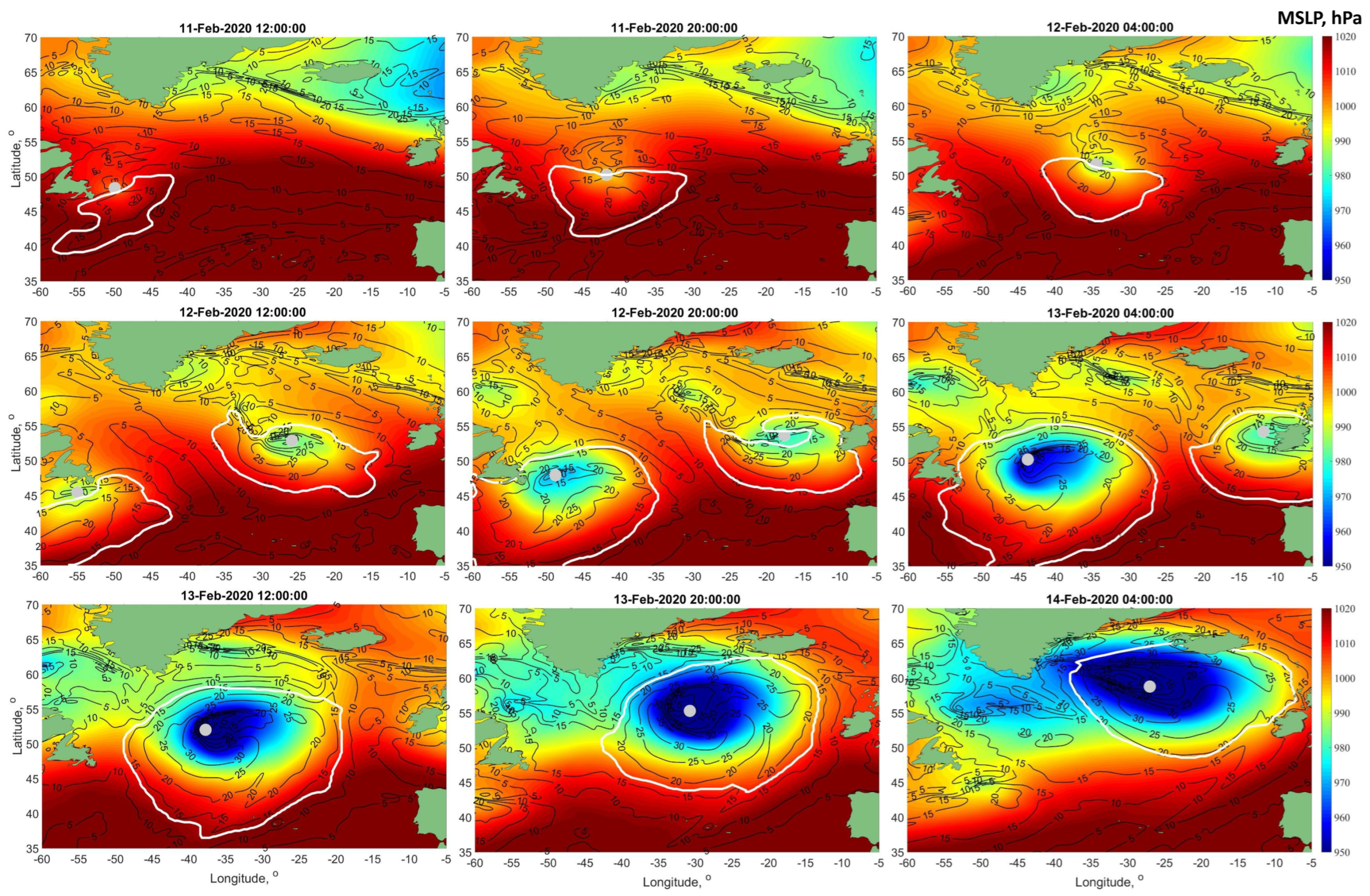
Based on the NCEP/CFSv2 hourly wind fields and surface pressure maps, two ETCs were identified moving simultaneously over the North Atlantic between 11 February 2020 and 15 February 2020, as seen in Figure 1. The first ETC (ETC#1) appeared on the morning of 11 February 2020, in the west of the basin at 48 degrees north latitude, and then moved east until it reached the coast of Ireland on the morning of 13 February 2020. The second ETC (ETC#2) also appeared in the west of the basin at 46°N, but a little later, at noon on 12 February 2020. Unlike the ETC#1, its movement was directed to the northeast, and when it reached 60 degrees north latitude at noon on 14 February 2020, ETC#2 lost shape and turned into an “air stream” along the southeast coast of Greenland and, eventually, continued to exist as the Icelandic low, as seen in Figure 1.

Figure 1. Mean sea level pressure, MSLP, maps with wind speed contours in ms${}^{-1}$. White contours are the storm area of ETCs with the gray circle as their center.

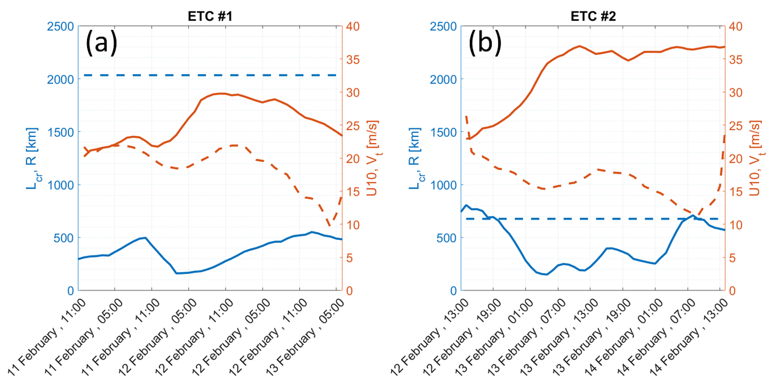
The coordinates of the minimum surface pressure were used to derive the center of ETCs, their trajectories, and then the translation velocities. The maximal value of wind speed in the vicinity of the ETC center, $u_m$, and the distance from the location of $u_m$ to the center, $R_m$, called as an analogy of Tropical Cyclones (TC) the maximum wind speed radius, are considered to be the main ETC parameters, characterizing its evolution. The ETC storm area is thus defined as the inner area around the ETC center where wind speed exceeds a given (threshold) value, which was empirically chosen as $max(0.45 u_m,12{\mathrm{ms}}^{-1})$.

The time evolution of $u_m$, $R_m$, and $V_t$, for ETC#1 and ETC#2 are shown in Figure 2a,b, respectively. The ETC#1 moves with average translation velocity, ${\overline{V}}_t$, equal to 19 ms${}^{-1}$. At the initial stage of the ETC#1 evolution, $u_m$ and $R_m$ are 20 ms${}^{-1}$ and 300 km, respectively. The largest values of $u_m$ and $R_m$ during its life span are $\sim 31$ ms${}^{-1}$ and 500 km, respectively, as seen in Figure 2a. The ETC#2 moves, with ${\overline{V}}_t$, equal to 17 ms${}^{-1}$. The maximum values of $u_m$ and $R_m$ during its life span are $\sim 40$ ms${}^{-1}$ and 700 km, as seen in Figure 2b.

Figure 2. Time evolution of ETC#1 (a) and ETC#2 (b) parameters: (red thick line) maximum wind speed, $u_m$; (red dashed line) translation velocity, $V_t$; (blue thick line) radius of maximum wind speed, $R_m$; (blue dashed line) critical fetch, ${\overline{L}}_{cr}$ from (1).

2.2. Measurements of Wave Parameters

2.2.1. Significant Wave Height

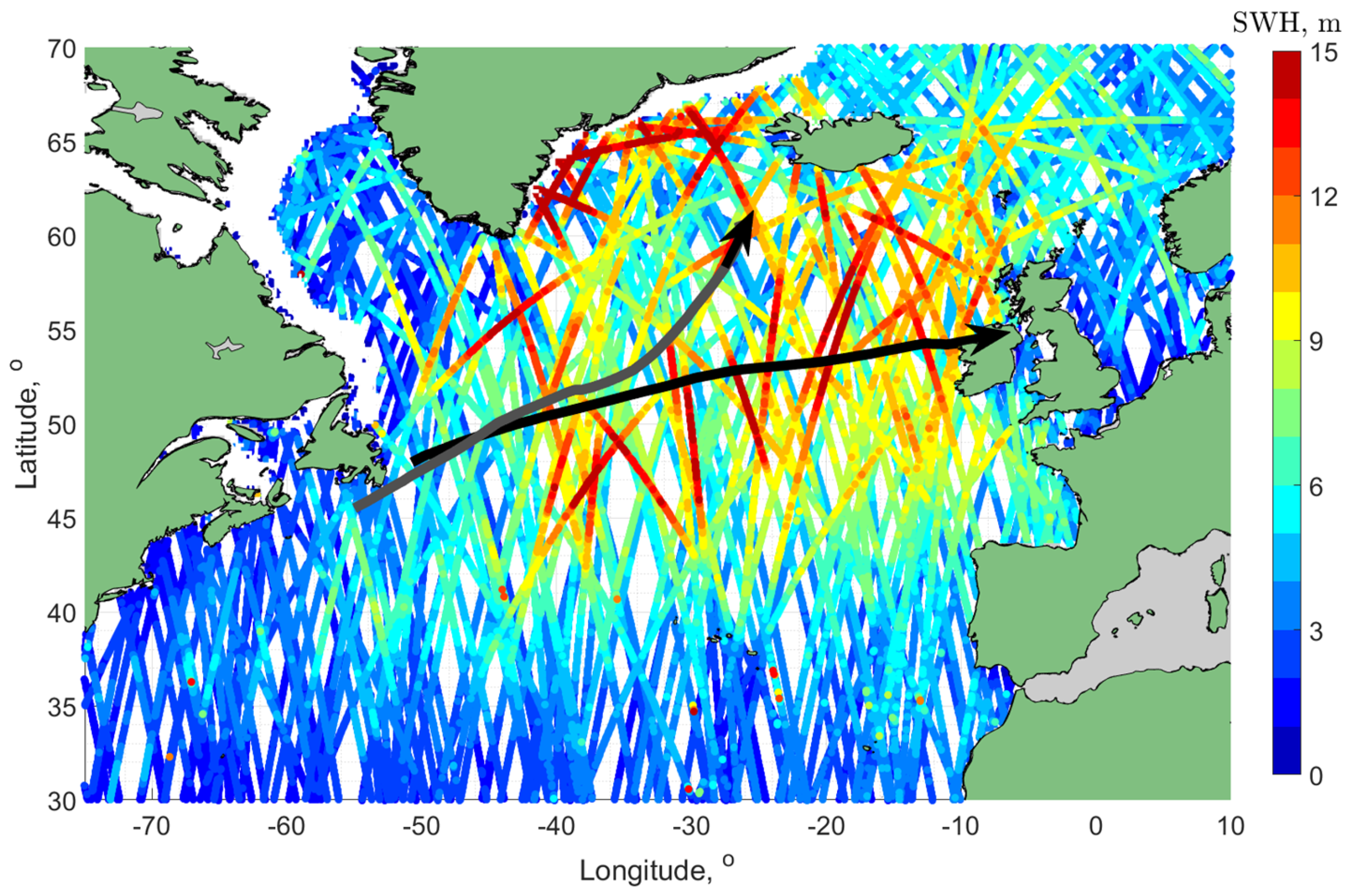
The measurements of significant wave height (SWH) are produced by different satellites, as shown in Figure 3. The SWH data used in this study include level two altimeter 1 Hz observations of Sentinel-3A, Sentinel-3B, Jason-3, CryoSat-2, AltiKa, and nadir nsec products of CFOSAT-SWIM, illustrated in Figure 3, with trajectories of ETCs. To show the SWH values, the land/ice mask and data quality flags are applied. Referring to Figure 3, one may find that the highest waves with SWH $>10$ m are observed around the ETCs tracks crossing the northern Atlantic Ocean. To analyze the SWH of waves generated by ETCs in more detail, the altimeter tracks which cross the storm areas of each of ETCs were selected and presented in Section 3.1.1.

Figure 3. Altimetry tracks passing through the Northern Atlantic during the period of 11 February 2020 00:00 UTC–16 February 2020 00:00 UTC, after applying ice and land masks. The black line shows the trajectory of the ETC#1 and the gray line ETC#2. The colour of the altimeter tracks indicates measured SWH in meters.

2.2.2. Wave Spectrum Measurements from CFOSAT-SWIM

The SWIM (Surface Waves Investigation and Monitoring) instrument is used by the China-France Oceanography Satellite (CFOSAT). SWIM is a Ku-band radar with nadir and near-nadir scanning beam geometry designed to measure the spectral properties of surface ocean waves [16]. Here, we use level two products processed by CNES and IFREMER: SWH, spectral peak wavelength, ${\lambda }_p$ and wave direction, ${\phi }_p$, with 180° ambiguity.

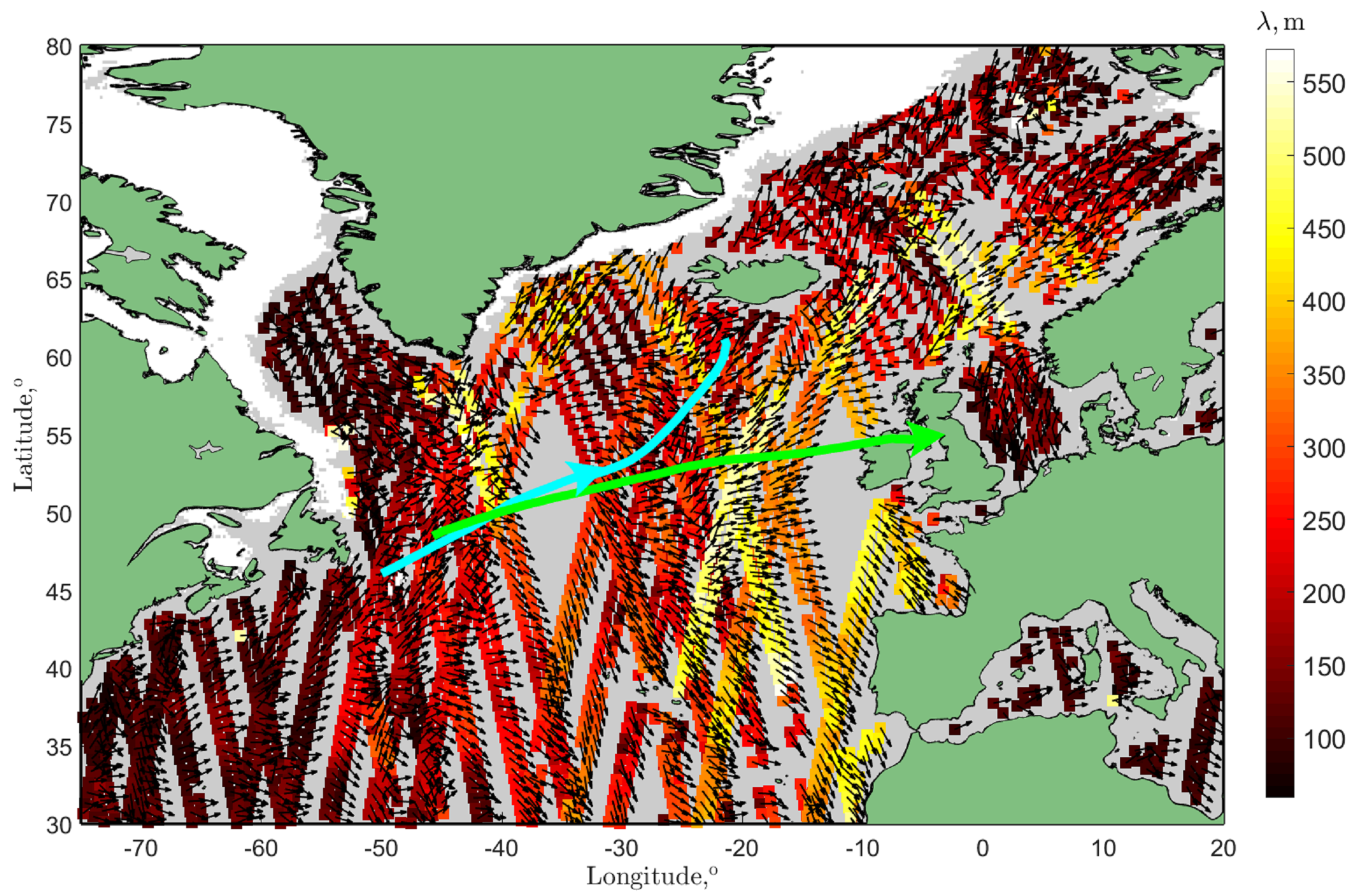
The SWIM nadir measurements of SWH are already shown in Figure 3 in combination with other altimeters observations. The SWIM estimations of ${\lambda }_p$ and ${\phi }_p$ are shown in Figure 4. To eliminate the 180° ambiguity of the SWIM wave direction, the wave directions were checked and corrected according to the corresponding wind directions, so that the wave direction is true when it is in the same quadrant with local wind directions taken from NCEP/CFSv2. Otherwise, the wave direction should be corrected by adding or subtracting 180° [34].

Figure 4. Measured ${\lambda }_p$ (colored boxes) and ${\phi }_p$ after eliminating 180° ambiguity (black arrows) in “wave boxes” on two sides of the CFOSAT-SWIM track in Northern Atlantic during the period of 11 February 2020 00:00 UTC —16 February 2020 00:00 UTC, after applying ice and land masks. The green and cyan colored lines and arrows show the trajectory and direction of the ETC#1 and ETC#2, respectively.

Although CFOSAT-SWIM l2 products, processed by CNES, give a wealth of information on the peak parameters, analyzing the wave spectrum using the l2s products processed by IFREMER is inevitable. The directional wave spectra are reconstructed from scanning radar measurements obtained with rotating beams directed at mean incidence angles of 0° (nadir), 2°, 4°, 6°, 8°, and 10°. In this study, we used observation from the angle of incidences 6°, 8°, and 10°.

3. Results: Features of Waves in Storm Area

The moving nature of cyclones leads to specific and important features of the generated wave fields. Specifically, waves generated in the right sector (where the wind is aligned with the cyclone heading) may stay under wind forcing for longer than in the left sector, where the wind is opposite to the cyclone’s heading. Wind waves in the right sector are thus often more developed than in the left one (as well as in comparison with a stationary cyclone), and hence are higher and have longer wavelength [18,19,20,21,22,26,27].

Differences between waves generated in the right sector, compared to those generated in the left one or in the case of a stationary cyclone, then depend on the relationship between the maximum wind speed, $u_m$, its radius, $R_m$, and velocity of cyclone movement, $V_t$. These parameters are combined in a critical length scale $L_{cr}$

$${\overline{L}}_{cr}=c_{cr}\frac{u_m^2}{g}{\left(\frac{u_m}{2V_t}\right)}^{1/q}$$

(1)

where $c_{cr}$ is a constant and q is the fetch-law exponent for the peak frequency, which following [23] are set here as: $c_{cr}=6.46\times {10}^3$ and $q=-1/4$.

The critical fetch $L_{cr}$ is the distance traveled by a developing train of waves from its point of origin to the point, where its group velocity reaches the value $V_t$ [22]. $L_{cr}$ thus helps divide all cyclones into two types: slow-moving if $R_m/L_{cr}>1$ and fast-moving if $R_m/L_{cr}<1$. In the former case, wind waves developing in the right sector can “outrun” the storm to become swell systems propagating ahead of the cyclone. In the latter case, the developing waves move backward relative to the cyclone and leave the storm zone through the rear sector, becoming trailing swell systems. A more detailed description of waves generated by different types of cyclones can be found in [23].

For the considering ETCs, an estimation of critical fetch, $L_{cr}$, can be achieved using the mean values of $V_t$ and $u_m$ which are: ${\overline{u}}_m=26$ m/s and ${\overline{V}}_t=19$ m/s for ETC#1, and ${\overline{u}}_m=34$ m/s and ${\overline{V}}_t=16.5$ m/s for ETC#2. The average values of critical fetch are ${\overline{L}}_{cr}\sim$2000 km and ${\overline{L}}_{cr}\sim$670 km for ETC#1 and #2, respectively, (Figure 2). Comparing ${\overline{L}}_{cr}$ with $R_m$ one may conclude that both ETC can be classified as fast-moving cyclones. In this case, we anticipate that the storm area in both ETC should be filled with developing wind waves. Following [22,23], the generation of these waves starts once the front boundary of the fast-moving storm appears at a given point. Since these developing waves are slow, they move backward relative to the traveling storm. These waves then attain a maximal development at the rear boundary of the storm, and then leave it, propagating behind as swell systems.

3.1. Profiles of Wave Parameters across ETCs

3.1.1. SWH

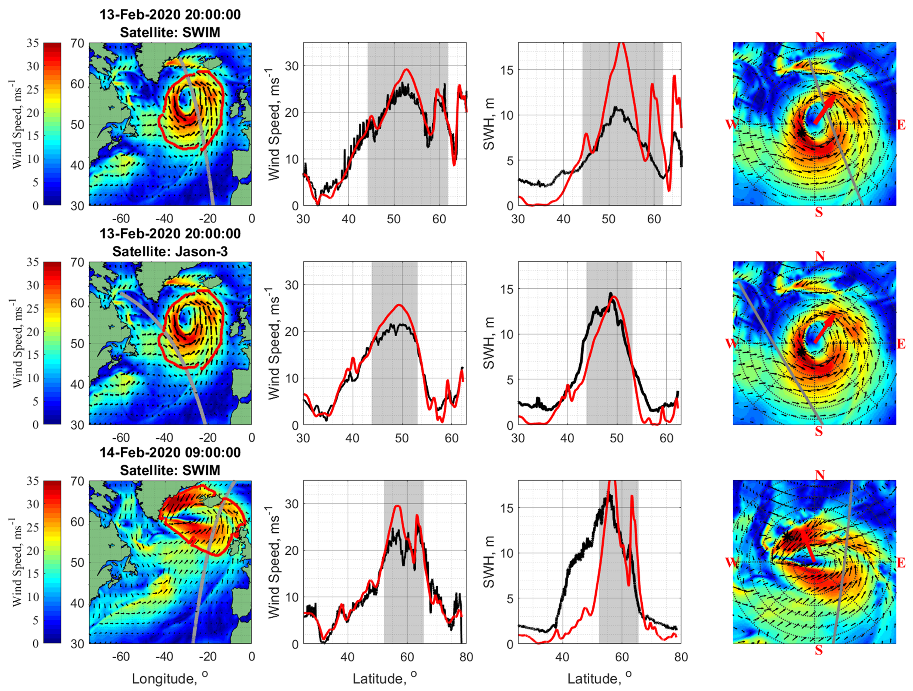
Among 130 altimeter tracks crossing the North Atlantic in the period 11–15 February 2020, 14 and 26 tracks crossed storms ETC#1 and ETC#2, respectively. Some of these tracks are displayed in Figure 5 for ETC#1 and Figure 6 for ETC#2, together with corresponding profiles of altimeter-derived wind speed and SWH (black lines), and cross-section profiles of the NCEP/CFSv2 wind speed and the SWH of fully developed seas, $H_s=0.21 u^2/g$ [35] along the selected altimeter tracks. Vertical shaded areas in columns 2 and 3 indicate the parts of the tracks crossing the ETCs’ storm area exactly, shown on the wind fields in the left column by a red contour.

Figure 5. Wind speed and SWH along the AltiKa, CryoSat-2, Sentinel-3, and CFOSAT-SWIM nadir tracks at the different moments of ETC#1 lifetime. Columns from left to right, (1st column): NCEP/CFSv2 wind field and position of the track; (2nd column): along-track wind speed from (black line) measurements and (red lines) NCEP/CFSv2; (3rd column): profile of measured SWH (black line) and SWH of fully-developed waves for local wind speed (red line); (4th column): zoom on the ETC#1 storm (inner) area (shown in the first column by red contour). The red arrows in the fourth column indicate the ETC’s direction, and the radius of dashed circles changes from 200 km at a 200 km interval. Vertical shaded areas in columns 2 and 3 indicate the parts of the tracks that fell into the ETC’s storm area, shown in the first column by red contour. The position of $u_m$ is indicated by a black asterisk.

Figure 6. The same as in Figure 5, but for ETC#2 and altimeters AltiKa, CryoSat-2, Sentinel-3, Jason-3, and CFOSAT-SWIM nadir tracks.

Referring to Figure 5 and Figure 6, wind fields in the ETCs show strong radial-azimuth asymmetry: strong winds in the right and rear sectors cover a larger area than in the front and left sectors. The wind speed estimates on the tracks crossing the ETC eye are also larger in the right sector than in the left. The difference of $u_m$ between these sectors does not exceed 10 ms${}^{-1}$. On the other hand, the difference in the maximum SWH values between the same sectors is much larger and exceeds the values that could be expected from the observed wind speed difference. In some cases, e.g., tracks of CryoSat-2 and Sentinel-3A in Figure 5 on 13 February at 21:00 and 23:00, the difference of SWH maxima between the right and the left sectors is about 10 m.

A zoomed-in version of the ETCs’ storm area (shown in the left column within the red curves) is presented in the last column of Figure 5 and Figure 6 in the orthogonal coordinates systems. The radius of gray circles in these plots changes from 200 km with a 200 km increment. The location of $u_m$ is shown by a black asterisk. After careful inspection of the wind speed and SWH profiles, in Figure 5 and Figure 6, the maximum SWH is found to be, in most cases, behind (upwind) the position of the maximum wind speed.

To help separate the measured SWH according to the type of surface waves, including developing wind waves, mature wind waves, and swell, a “threshold” SWH is introduced as

$$H_{s_{fd}}=0.21 u^2/g,$$

(2)

which corresponds to the SWH of fully developed waves [35]. Consequently, observed waves with SWH $H_s<H_{s_{fd}}$ can be considered to be developing waves, and waves with SWH $H_s>H_{s_{fd}}$—as swell. The NCEP/CFSv2 wind speed is further used as the reference to calculate $H_{s_{fd}}$.

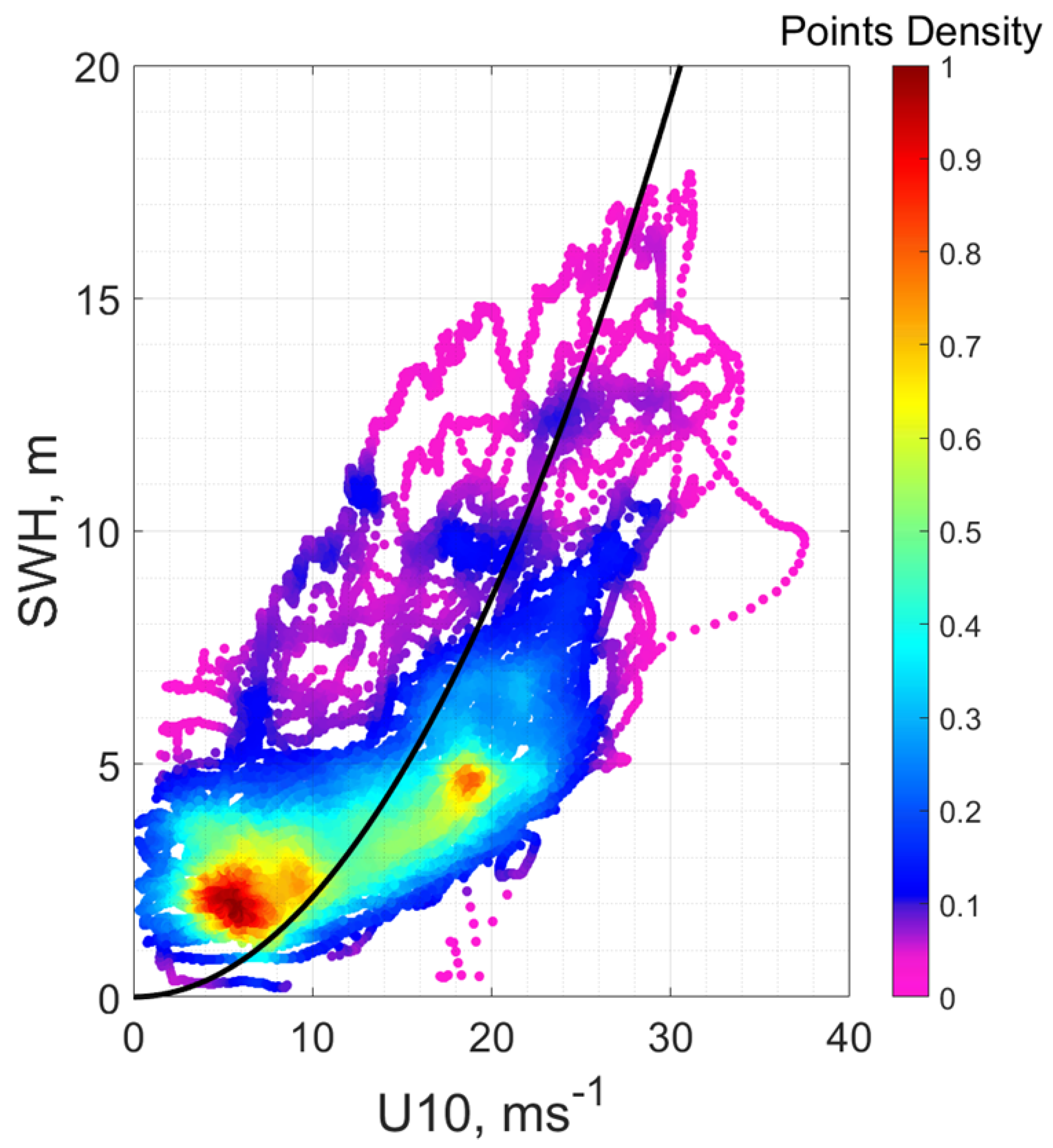
Comparison of the measured SWH with $H_{s_{fd}}$, Figure 5 and Figure 6, indicates that observed waves in the inner storm area can be classified as developing and mature wind waves, and waves outside the storm area can be interpreted as swell. All the data shown in Figure 5 and Figure 6, are presented in Figure 7 as a scatter plot “SWH vs. wind speed”. The measured SWHs below the “threshold” line from (2) represent wind waves developing under local wind forcing, and SWHs above—represent swells that travel outside the storm area.

Figure 7. Two−dimensional scatter plot of significant wave height SWH as a function of wind speed, colored with points density. The black curve shows the $H_{s_{fd}}=0.21 u_{10}^2/g$ [35].

3.1.2. Spectral Peak Parameters

From 11–15 February 2020, about 30 CFOSAT-SWIM tracks crossed the North Atlantic, as shown in Figure 4. However, only 3 and 4 tracks perfectly crossed the storm area of ETC#1 and ETC#2, respectively. Some of those tracks are shown in Figure 5, for ETC#1 and Figure 6, for ETC#2, together with corresponding profiles of wind speed and SWH. Hereafter, we solely analyze the parameters of the spectral peak—wavelength and direction.

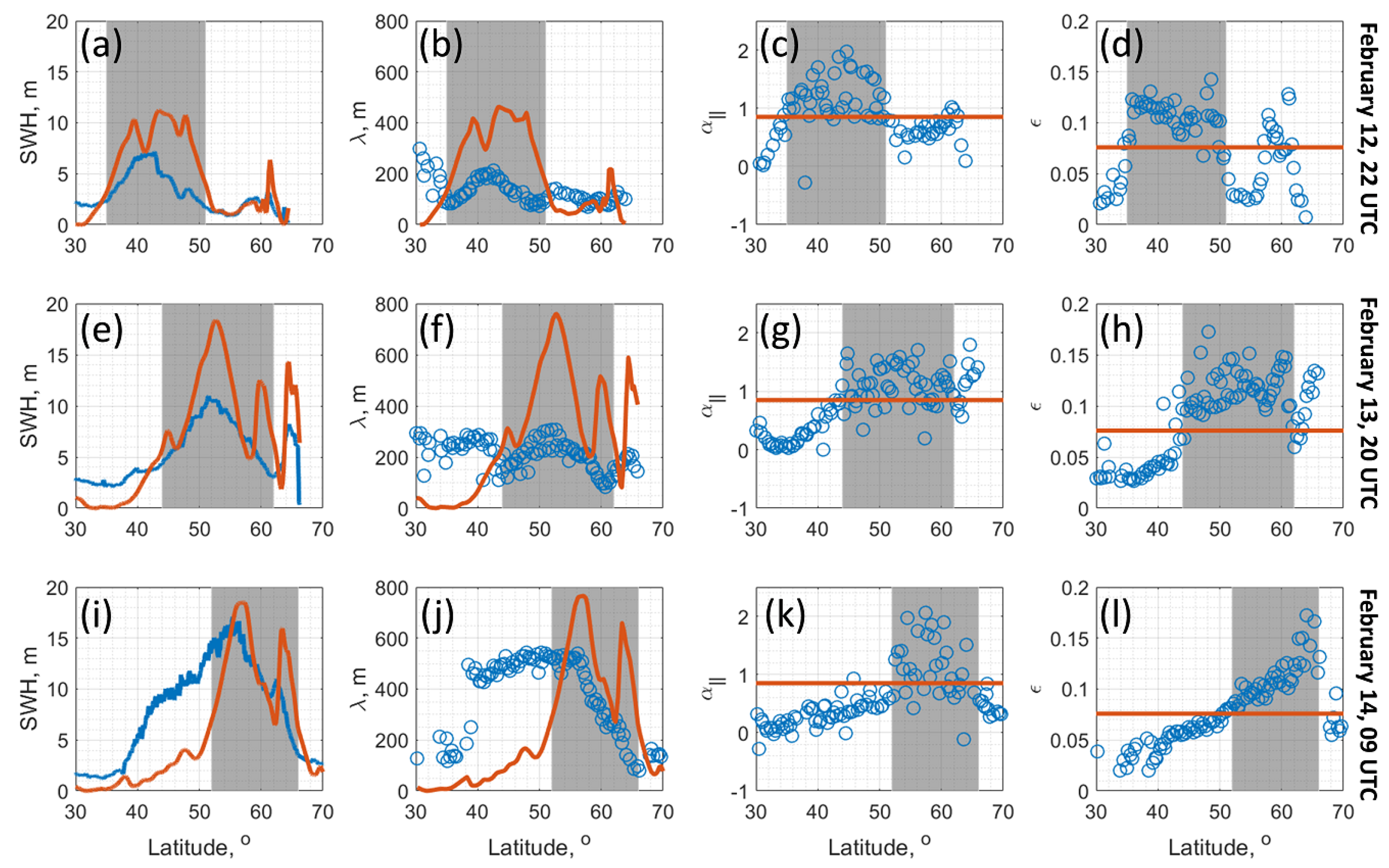
The measured along-track SWIM nadir SWH, off-nadir wavelength of a spectral peak, ${\lambda }_p$, and wave significant steepness, $ϵ=k_p{H}_s/2$, for cases on 12 February, 22 UTC,13 February, 20 UTC, and 14 February, 09 UTC are presented in Figure 8 (blue points). The satellite nadir track for these cases is shown on the maps of the 2nd, 8th, and 10th rows, as shown in Figure 6. The orange lines in each panel of Figure 8, show SWH, $H_{s_{fd}}=0.21 u_{10}^2/g$, wavelength, ${\lambda }_p=(2\pi /0.85)u_{10}^2/g$, and significant steepness, ${ϵ}_p=k_p{H}_s/2=0.076$, for fully developed waves. These estimates are used as reference values to discriminate between wind, seas, and swells. Observed waves are classified as wind waves (resp. swell) if their measured SWH and wavelength are less (resp. larger) than these reference values. For the significant steepness, the situation is reversed, i.e., the larger values are attributed to wind waves and the smallest to swell. Such a separation based on threshold reference values appears surprisingly well consistent with direct estimates of local inverse wave age, ${\alpha }_{\left|\right|}=(u/c_p)cos({\phi }_p-{\phi }_w)$, shown in Figure 8, where $c_p=\sqrt{g{\lambda }_p/2\pi }$ is the peak phase velocity, ${\phi }_w$ and ${\phi }_p$, the directions of the local wind and the spectral peak, respectively.

Figure 8. Along−track profile of (a,e,i) SWHs, $H_s$; (b,f,j) spectral peak wavelength, ${\lambda }_p$; (c,g,k) inverse wave age,${\alpha }_{\left|\right|}=(u/c_p)cos({\phi }_p-{\phi }_w)$; and (d,h,l) wave steepens, $ϵ=k_p{H}_s/2$ with $k_p=2\pi /{\lambda }_p$. Blue circles and curves show the measurements, and the orange curves represent the values associated with fully developed waves. The average time of the SWIM passage over the North Atlantic Ocean is shown on the right side of each row. The SWIM nadir tracks can be found in 2nd, 8th and 10th rows of Figure 6.

A remarkable feature, shown in Figure 8, is that locations of wind-driven waves and swells detected by different instruments (nadir altimeters and radar SWIM) for different wave parameters (SWH, ${\lambda }_p$, ${ϵ}_p$, ${\phi }_p$ ) are very consistent. It suggests that the inner storm area of fast-moving ETC is dominated by developing waves. Although this statement sounds trivial, it is an important feature of the wave field in fast-moving cyclones. In the case of slowly moving cyclones with parameters satisfying condition $R_m/L_{cr}>1$, the primary wave system, represented by developing wind waves, occupies a limited area in the front-right sector, and in the rest of the area the primary wave system is represented by swells (see [23] and their Figure 10 for illustration).

3.2. Spatial Distributions in the ETC Storm Area

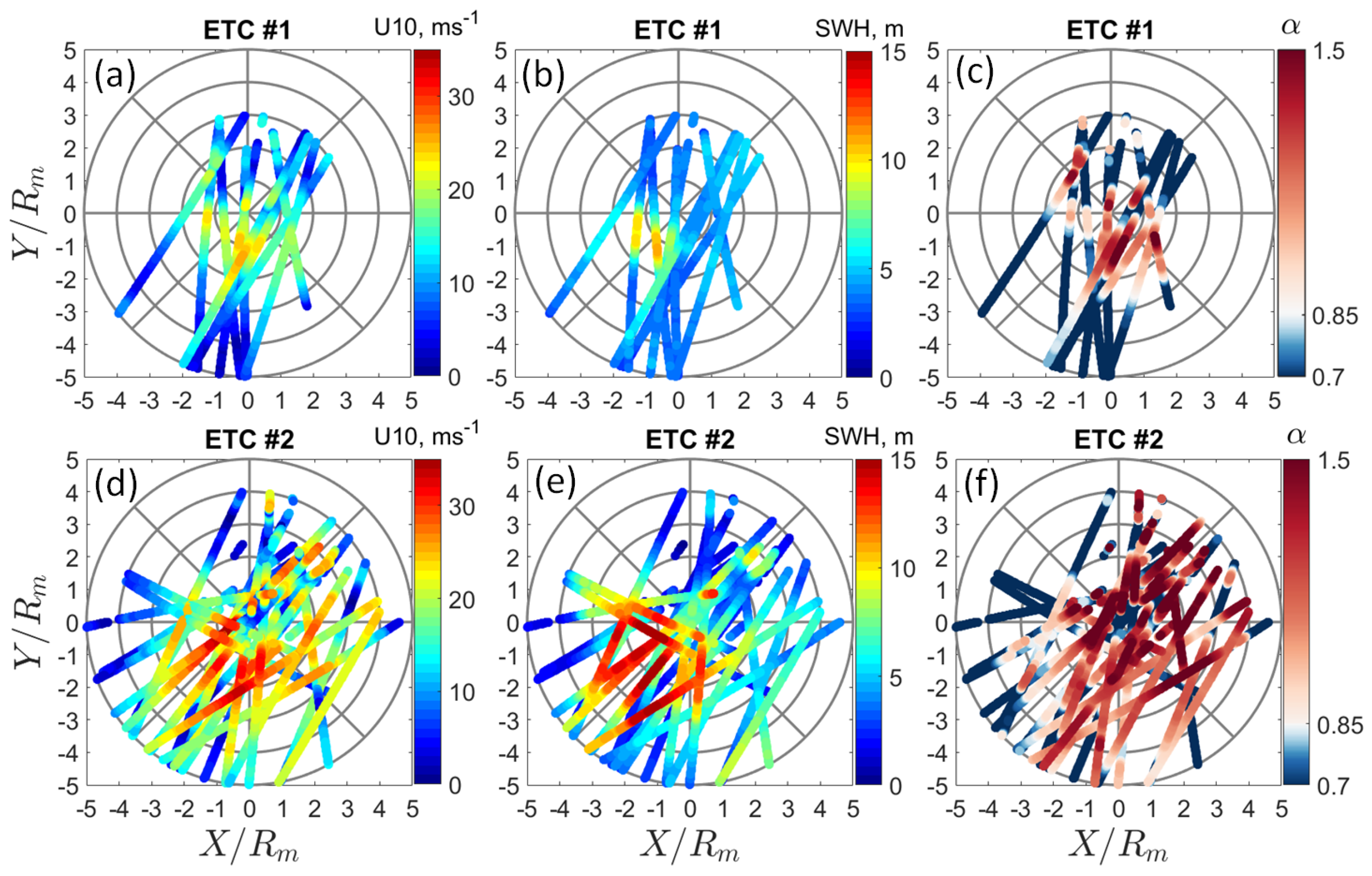
To better understand wind waves under these ETCs, the along-track distributions of wind speed and SWH are displayed in Figure 9, in a rectangular coordinate system with the origin tied to the eye of the ETC moving in the x-direction. Figure 9a,d confirm that the wind is stronger in the rear-right sectors of both ETCs. This is consistent with [36], who analyzed wind speed fields in ETCs to reveal systematic asymmetries with maximum wind speed in the rear-right quadrant.

Figure 9. Along−track wind speed, SWH, and $\alpha$ inside the cyclone in a coordinate system associated with the coordinates of ETCs considering their heading aligned in x-direction, respectively, illustrated in (a–c) for ETC#1 and (d–f) for ETC#2.

Spatial distributions of SWH, shown in Figure 9b,e, exhibit higher values in the rear-right quadrant at a radial distance about $1<r/R_m<3$. In our case, the largest surface waves approximately coincide with the area of higher wind speeds. On the one hand, relative SWH enhancements in the same quadrant were reported by [2,37] using numerical simulations. This is consistent with predictions of the self-similarity theory of wave development in moving storms based on the extended fetch concept [19,21,23]. This mechanism suggests that in the right sector, where wind direction coincides with ETC heading, developing waves stay under wind forcing for longer. Wave energy can then accumulate compared to other sectors or become a stationary storm with the same $u_m$ and $R_m$.

It is then tempting to quantify waves generated by ETCs in terms of inverse wave age. One of the fundamental results of the similarity theory for the wave growth by [38], is the proportionality of the dimensionless energy, $\tilde{e}=e{g}^2/u_{10}^4$, to the inverse wave age, $\alpha =u_{10}/c_p$ (which is equal to dimensionless peak frequency), to some certain power, e.g., to a power of “−3”: $\tilde{e}\propto {\alpha }^{-3}$ [39]. Using the definition $e=H_s^2/16$, the relationship between inverse wave age and SWH reads:

$$\alpha =0.85{\left(\frac{{\tilde{H}}_{s_{fd}}}{{\tilde{H}}_s}\right)}^{2/3},$$

(3)

where $H_{s_{fd}}$ and $0.85$ are SWH and inverse wave age corresponding to fully developed seas, respectively.

The inverse wave age maps, as seen in Figure 9c,f, show that the inverse wave age estimate, found in the right sector and partly in the left one, is $\alpha >0.85$. This suggests that waves in the inner storm area (inside $r/R_m\le 4$ for ETC#2 and $r/R_m\le 2$ for ETC#1) are developing mature wind waves. This is likely because the analyzed ETCs are fast-moving systems, with their $R_m$ smaller than the critical fetch $L_{cr}$ estimate, see Figure 2. In this case, waves start to develop in the forward sector, at the same time that the storm area appears at a given point in the ocean. The group velocity of the waves is then less than the ETC translation velocity, and the developing wind waves move backward relative to the ETC. Waves finally radiate out of the storm area through its rear boundary. This can be seen in Figure 9, in reasonable agreement with the simulations of wave generation under fast-moving cyclones, Ref. [23] (see their Figure 9d,h).

3.3. SWH Time Evoloution

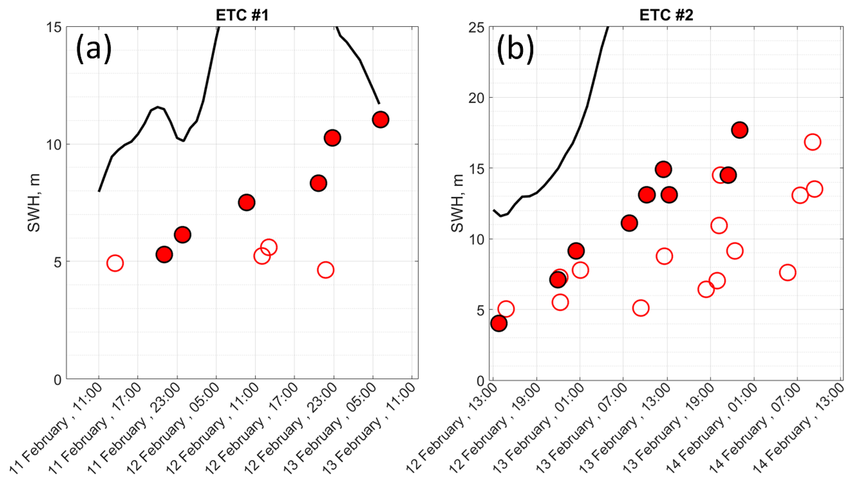
Data

Figure 10a,b display the time evolution of the maximal values of SWHs on each of the altimeter tracks, shown before in Figure 9c,d. The highest waves, maximal SWHs, are again divided into developing wind waves, whose local inverse wave age is $\alpha >0.85$, and swell, $\alpha <0.85$. Distinctive characteristics are indicated in Figure 10a,b by the filled and open red circles. Fully developed wave heights, $H_{s_{fd}}=0.21 u_m^2/g$, calculated by [35] for the maximal local wind speed, are also presented in Figure 10a,b. Hereinafter, only wind waves are considered.

Figure 10. Time evolution of maximum SWH values for ETC#1 (a) ETC#2 (b). The filled red circles are related to the SWH of wind waves ($\alpha >0.85$), and the open red circles—to the SWH of swell. The black curves show the SWH of fully developed waves calculated for local $u_m$.

Wind wave SWH for the ETC#1 (Figure 10a) demonstrates a gradual increase. By the end of the ETC life, the level of fully developed waves is almost reached. Yet, this is mainly due to a decrease in wind speed. For ETC#2, the SWH trend is more pronounced. However, the observed SWHs are still well below the fully developed level (black curve in Figure 10b).

4. Discussion

To qualify and quantify waves generated by ETCs, it is first tempting to consider the extended fetch concept, successfully applied to describe the waves generated by TCs [18,19,20,21,23,26]. This approach suggests that classical self-similar laws of wave growth by [38],

$${\tilde{\omega }}_p\equiv \alpha =c_{\alpha }{\tilde{x}}^q,\tilde{e}=c_e{\tilde{x}}^p,$$

(4)

can also be applied, with the wind fetch, $\tilde{x}=xg/u^2$, more properly defined to take into account TC’s moving nature. Such a fetch is termed an effective or an extended fetch [18,19,20,26]. In Equation (4), $\alpha$ is the inverse wave age, equal to the dimensionless spectral peak frequency, $\tilde{e}=e{g}^2/u^4$ is dimensionless energy, p and q are the fetch-law exponents, and $c_{\alpha }$ and $c_e$ are the constants. Examples of an application of self-similar laws for a description of waves in moving cyclones (either in radial and in the azimuthal directions) can be found in [23,25].

Following [23] (see their Equation (18)), the effective (extended) fetch, ${\tilde{X}}_e=Xg/u_m^2$, can be parameterized in self-similar variables as:

$$\begin{array}{c}\hfill {\tilde{X}}_e=1.1 {\tilde{R}}_m{[l_e+m_e{({\tilde{R}}_m/{\tilde{L}}_{cr}^m)}^{n_e}]}^{1/p},\\ \hfill {\tilde{X}}_{\lambda }=1.8 {\tilde{R}}_m{[l_{\lambda }+m_{\lambda }{({\tilde{R}}_m/{\tilde{L}}_{cr}^m)}^{n_{\lambda }}]}^{-1/2q}\end{array}$$

(5)

where [$l_e,m_e,n_e$] and [$l_{\lambda },m_{\lambda },n_{\lambda }$] are the constants, which depend on the type of storm. For slow-moving storms, ${\tilde{L}}_{cr}/{\tilde{R}}_m^{}\ge 1$, these constants are [1, 3.84, −0.4] and [1, 1.37, −0.38] for energy and wavelength, respectively. For fast-moving storms, ${\tilde{L}}_{cr}/{\tilde{R}}_m^{}<1$, these constants are correspondingly changed to [0, 2.92, 0.53] and [0, 1.67, 0.31].

In Figure 11, the waves, generated by ETCs, exhibit clear development in time. The developing waves suggested likely have not reached the steady state predicted by (5) with (1). Until they reach the steady solutions (5), the wave development must obey duration-laws, which in the framework of the classical self-similarity theory are:

$$\begin{array}{c}\hfill {\omega }_{p}u/g=c_{{\alpha }_t}{\left(tg/u\right)}^{q_t},\\ \hfill e{g}^2/u^4=c_{e_t}{\left(tg/u\right)}^{p_t},\end{array}$$

(6)

where $q_t$ and $p_t$ are duration law exponents, linked to the fetch law constants as follows: $q_t=q/(1+q)$ and $p_t=p/(1+q)$. The constants ${\alpha }_t$ and $c_{e_t}$ are also linked to the corresponding fetch-law constants (see, e.g., Equation (3) from [23]). Following [23], we adopt Toba’s fetch laws [39] with exponents $p=-1/4$ and $p=3/4$, which lead to duration laws exponent in (6) equal to $q_t=-1/3$ and $p_t=1$.

Figure 11. Dimensionless energy, $\tilde{e}$, versus dimensionless time, $\tilde{t}$, for ETC#1 (a) and ETC#2 (b): red circles are observations, and green lines are duration laws (6). Dashed-black and dashed-blue lines indicate the dimensionless time interval $t_0$ and $t_{max}$ defined by (7) and (8), and corresponding dimensionless energy predicted by duration laws (6).

The wave development will continue until the wave parameters reach the steady solutions (4) with (5). The required time interval, $t_{max}$, can be defined from the combination of duration laws (6) and the steady state values, (4) with (5), to give:

$$\begin{array}{c}\hfill t_{\lambda }^{max}=t_0{\left(l_{\lambda }+m_{\lambda }{\left(R_m/L_{cr}\right)}^{n_{\lambda }}\right)}^{-1/2q_t},\\ \hfill t_e^{max}=t_0{\left(l_e+m_e{\left(R_m/L_{cr}\right)}^{n_e}\right)}^{1/p_t},\end{array}$$

(7)

where $t_0$ is the timescale of wave development for a stationary storm, expressed through its radius as:

$$t_{0}g/u_m={\left(c_{\alpha }/c_{{\alpha }_t}\right)}^{1/q_t}{R}_m^{q/q_t}.$$

(8)

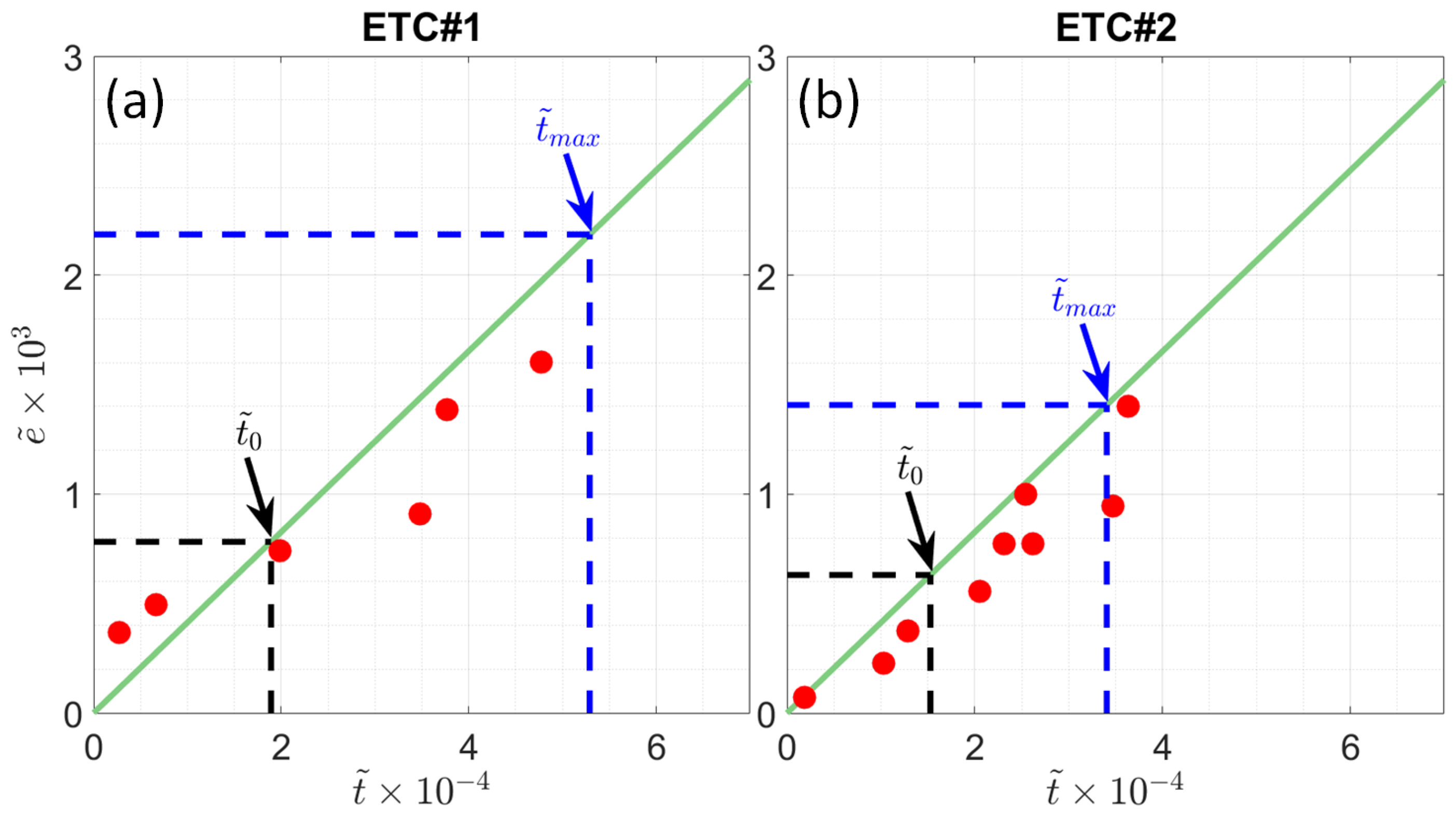
The dimensionless energy estimates, $\tilde{e}=e{g}^2/u_m^4$ (where $e=H_s^2/16$, as a function of dimensionless time, $\tilde{t}=tg/u_m$, where the mean maximal wind speed, ${\overline{u}}_m$, during the life span of each of ETCs is used for scaling, are shown in Figure 11a,b. The initial epochs of wave development, on 11 February 2020 at 19:00:00 for ETC#1 and 12 February 2020 at 12:00:00 for ETC#2, are chosen to fit the observations best. Duration laws (6), also shown in the same figure, exhibit an overall good agreement with the observations. Correlation coefficient of $\tilde{e}$ obtained from observations and Equation (6) is $\sim 0.95$ for both ETCs.

Two key time-scales, namely time intervals required to reach the steady state in stationary ETC, ${\tilde{t}}_0=t_{0}g/u_m$ defined by (8), and in moving ETC, ${\tilde{t}}_{max}=t_e^{max}g/u_m$ defined by (7), are shown in Figure 11a,b.

To estimate $t_0$, we used the values of $R_m$ and $u_m$ averaged over the lifespan of each ETC: ${\overline{u}}_m=26$ ms${}^{-1}$ and ${\overline{R}}_m=350$ km for ETC#1, and ${\overline{u}}_m=34$ ms${}^{-1}$ and ${\overline{R}}_m=450$ km for ETC#2. These values give $t_0\approx 14$ h and $t_0\approx 15$ h for ETC#1 and ETC#2, respectively. On the other hand, to estimate $t_e^{max}$, we used the values of $R_m$, $u_m$, and $V_t$ at the latest stage of the lifespan of ETCs, extracted from Figure 2 as [$u_m=24$ ms${}^{-1}$; $R_m=480$ km; $V_t=13$ ms${}^{-1}$], and [$u_m=36.5$ ms${}^{-1}$; $R_m=500$ km; $V_t=18$ ms${}^{-1}$], for ETC#1 and ETC#2, respectively. It gives $t_e^{max}\approx 39$ h and $t_e^{max}\approx 33$ h for ETC#1 and ETC#2, respectively. Referring to Figure 11a,b, we may find that neither wind waves developing under ETC#1 nor ETC#2 can attain the energy level predicted by the extended fetch relationship. Thus, wind wave development in the storm area of fast-moving ETC can better be considered to obey the classical duration laws. The effect of the fast-moving nature of the ETC on the growth of waves is to increase the residence time of waves under wind forcing. The longer this time, the more developed and higher the waves. This phenomenon, by analogy with extended fetch, can be called extended duration, similar to what was observed for waves generated by PLs [28].

5. Conclusions

Using multi-satellite measurements, this paper presents the results of investigating the main characteristics of the wind wave field generated by fast-moving ETCs in the North Atlantic. The two considered ETCs were fast-moving cyclones, in the sense that resonance (synchronism) between the group velocity of the generated waves and the ETC translation velocity is impossible. In this case, wave generation begins when the front boundary of the storm area crosses a given location in the ocean. Since the group velocity of the waves is always less than the ETC translation velocity, the developing waves move backward relative to the ETC, grow in time, and then leave the storm area through its rear sector. Multi-satellite observations confirm such a paradigm, and confirm that the main storm area is filled with young developing wind waves. The most developed waves are found in the moving ETC’s rear-right sector. Moreover, the energy of these waves grew with time during the ETC’s life span. In this context, observed wave fields in ETC are remarkably different from those generally associated with a TC. For latter cases, waves are usually enhanced in the right-front sector and demonstrate quasi-stationarity. As a consequence, the extended-fetch approach, commonly used to describe waves under TC, is not applicable for ETC. Instead, the concept of extended duration is more relevant, similar to what has already been found in PLs [28]. In this case, the moving nature of the ETC increases the residence time of waves under wind forcing. Satellite observations confirm the validity of duration-laws for waves generated by the ETC, and demonstrate that the extended-fetch regime for observing waves can only be asymptotically achieved at time intervals exceeding the lifespan of considered ETCs.

A more detailed description of the surface wave field characteristics generated by ETC, based on the use of parametric model simulations and satellite observations, will be discussed in the companion paper PART II [40].