
Satellite, UAV, and Geophysical Data to Identify Surface and Subsurface Hydrodynamics of Geographically Isolated Wetlands: Understanding an Undervalued Ecosystem at the Atlantic Forest-Cerrado Interface of Brazil

 ,
,
Abstract

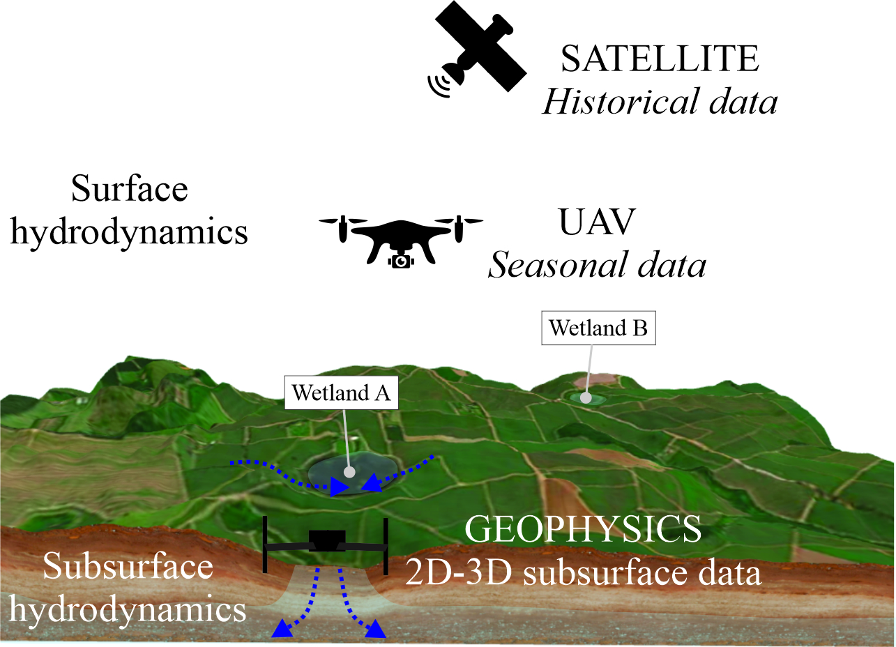
1. Introduction
2. Materials and Methods
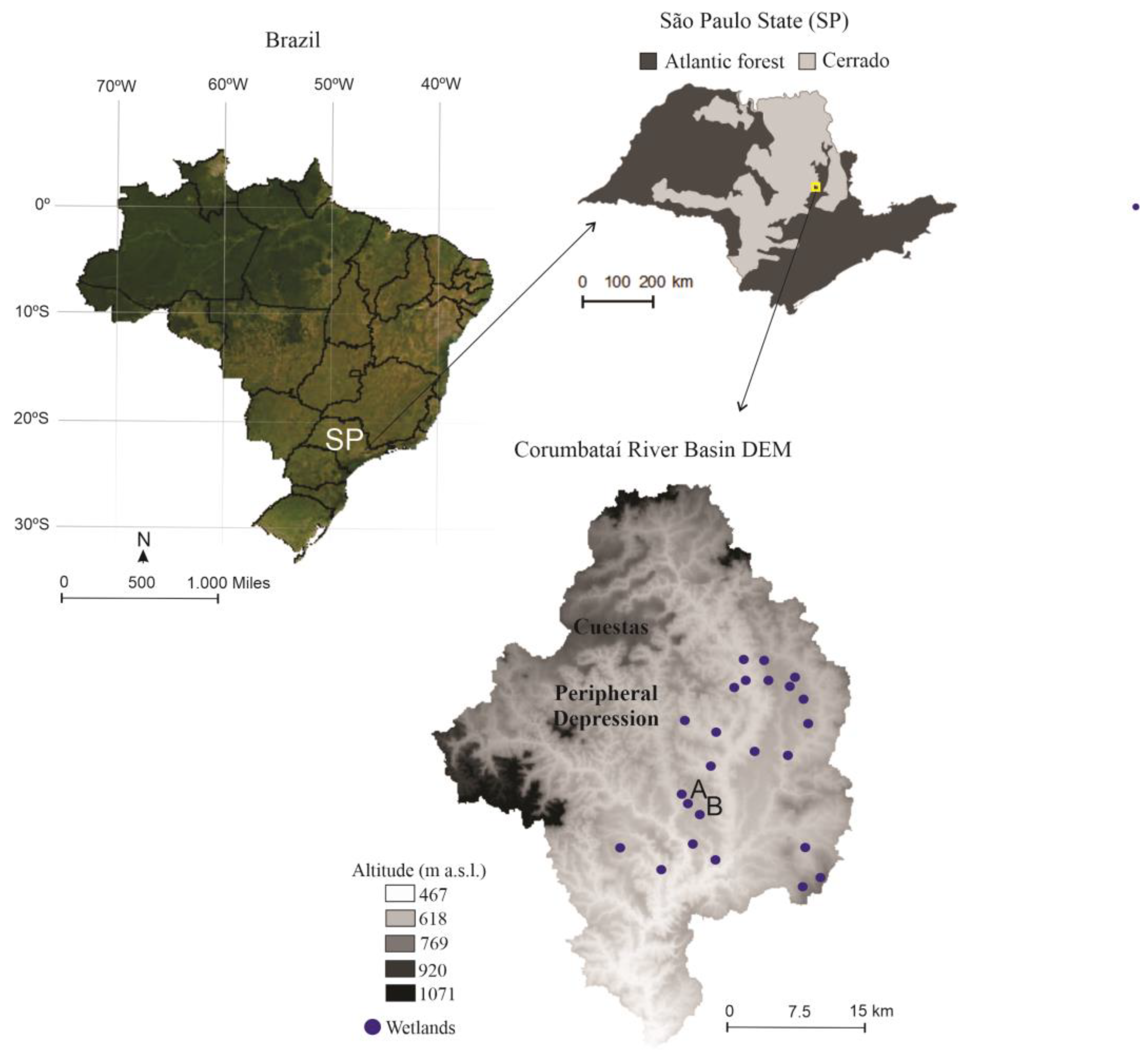
2.1. Study Sites
- (i)
- Wetland A: latitude: 22°25′41″S; longitude: 47°37′52″W; altitude: 610 m.
- (ii)
- Wetland B: latitude: 22°26′24″S; longitude: 47°37′8″W; altitude: 610 m.
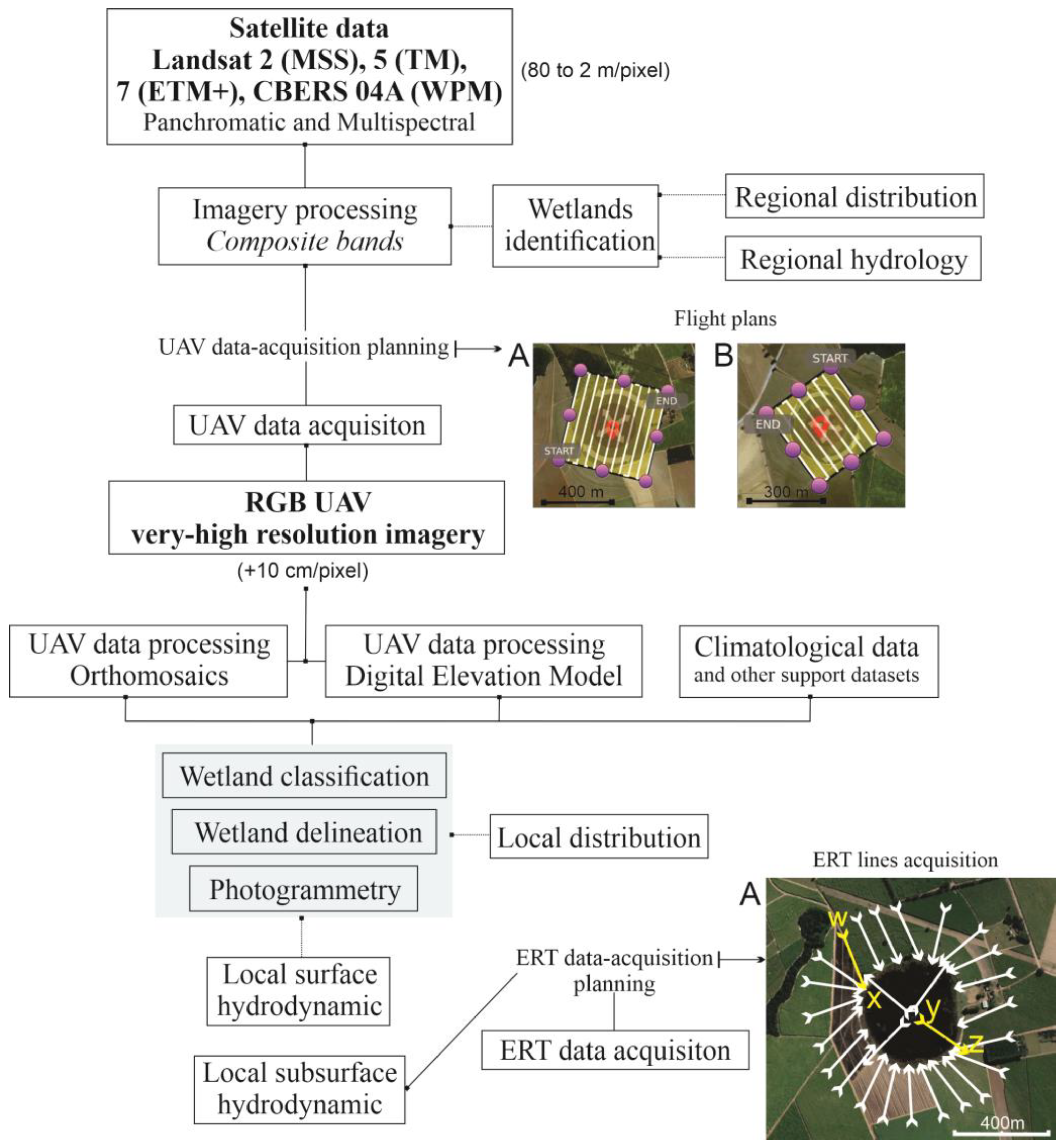
2.2. Satellite Images Acquisition and Bands Composition
2.3. UAV Data Acquisition and Processing
2.4. Water Balance for Hydrodynamic Analysis
2.5. ERT Geophysical Data Acquisition and Processing
3. Results
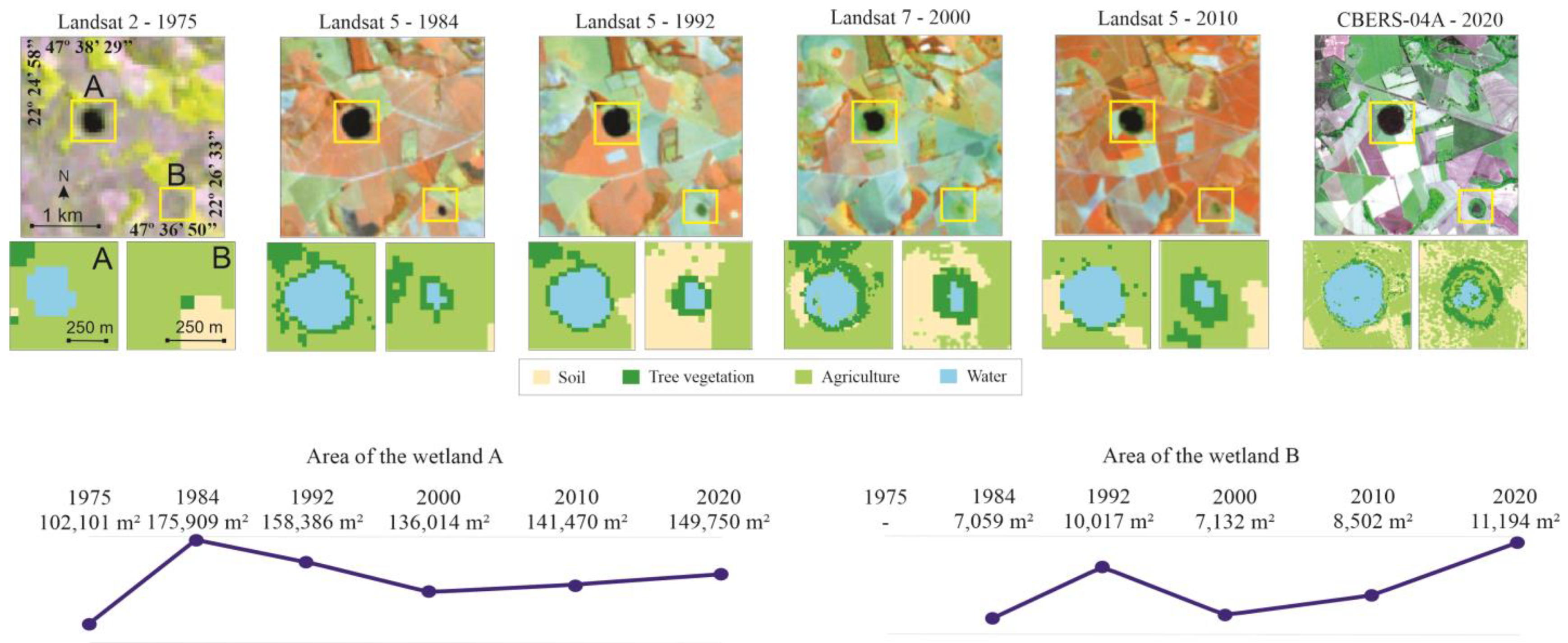
3.1. Satellite Products
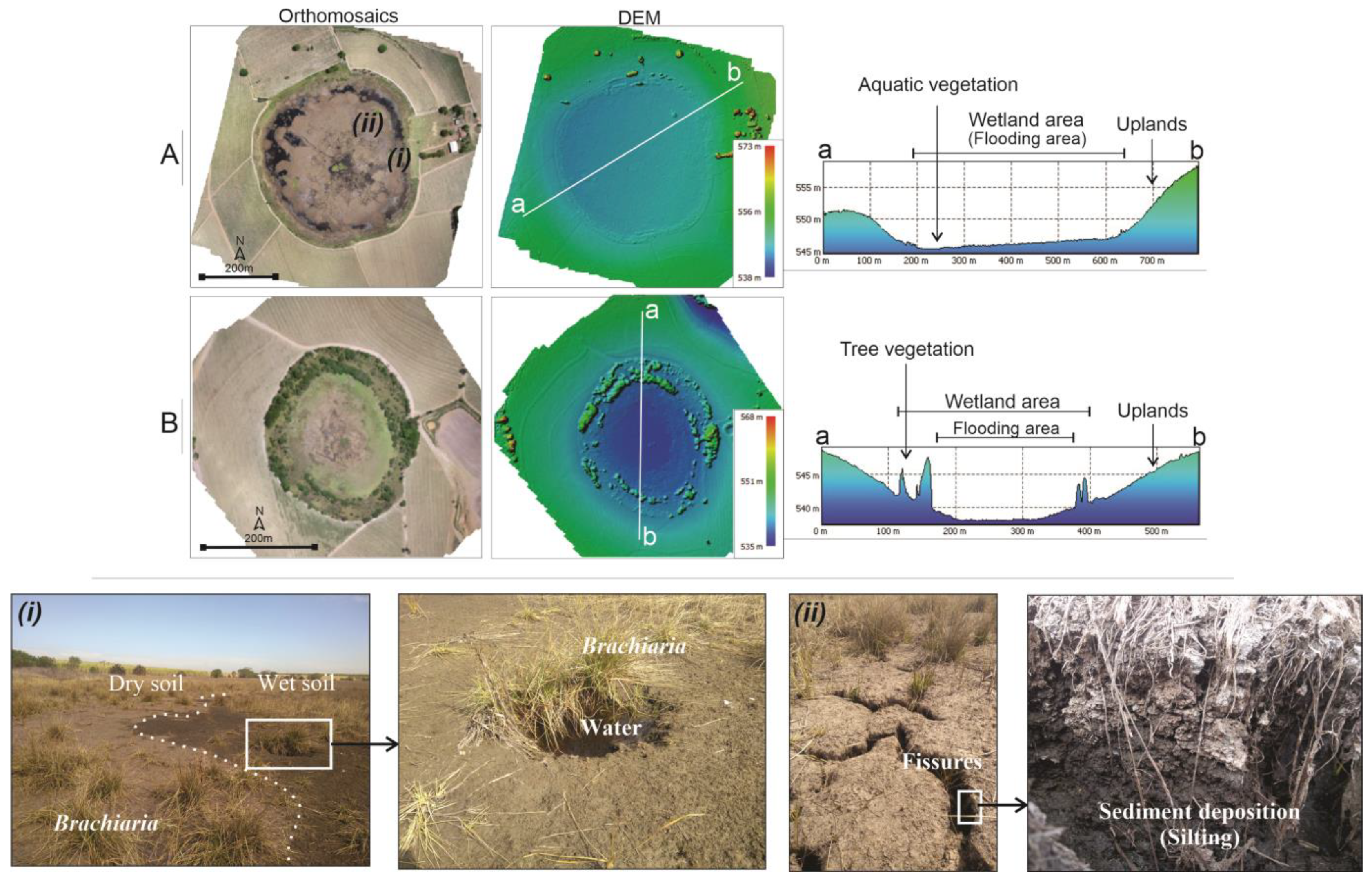
3.2. UAV Very-High-Resolution Orthomosaics and Digital Elevation Models
- (i)
- Dry-season images of wetland A. Dry and wet soil contrasts; Zoom-in, a water storage portion and native grasses tolerant to flooding;
- (ii)
- Soil-fissures observed in the border of wetland A; Zoom-in, where sediment deposition inside the wetland is observed (silting process).
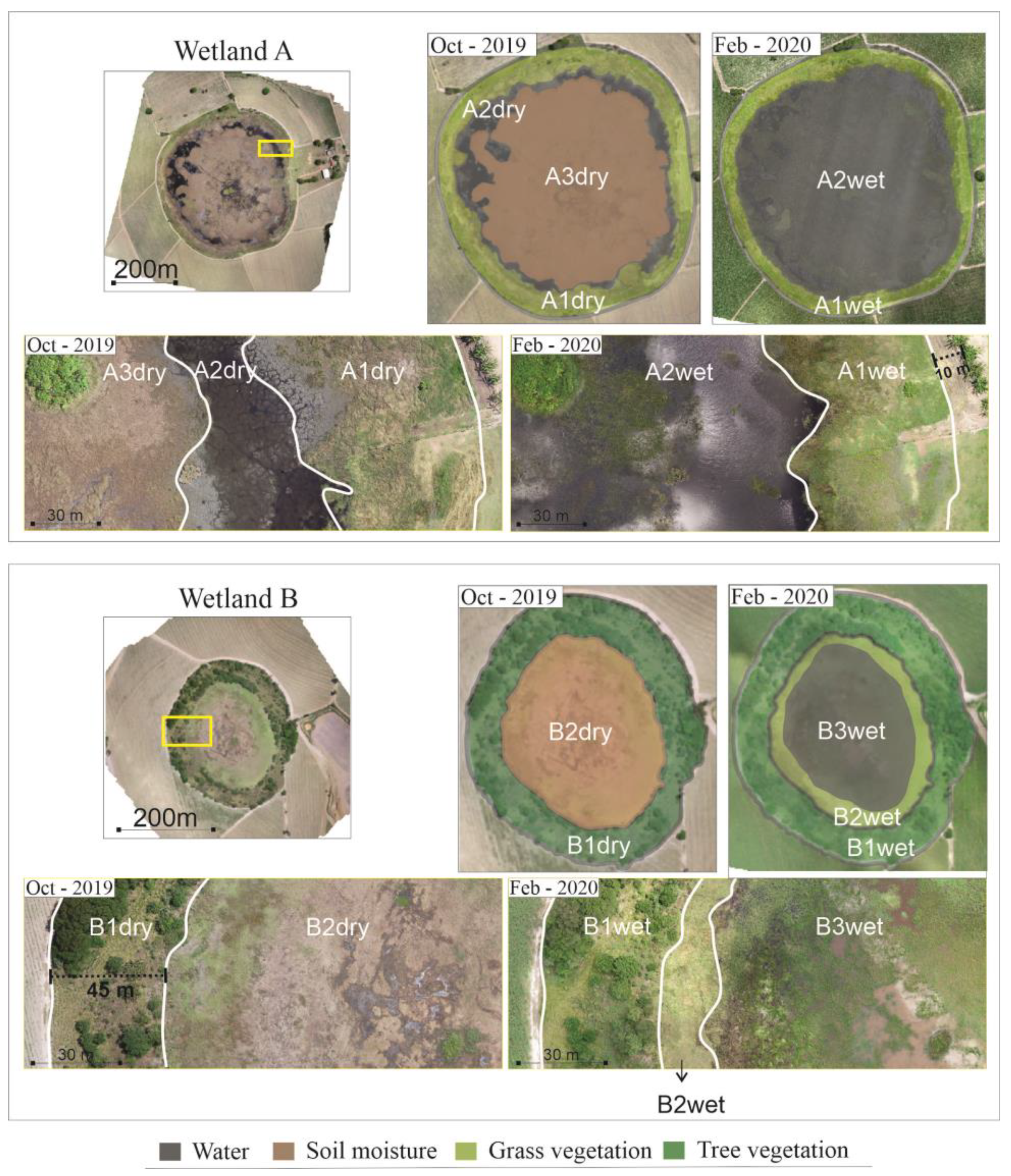
3.3. Water-Balance Integrated to Orthomosaics Imagery Response
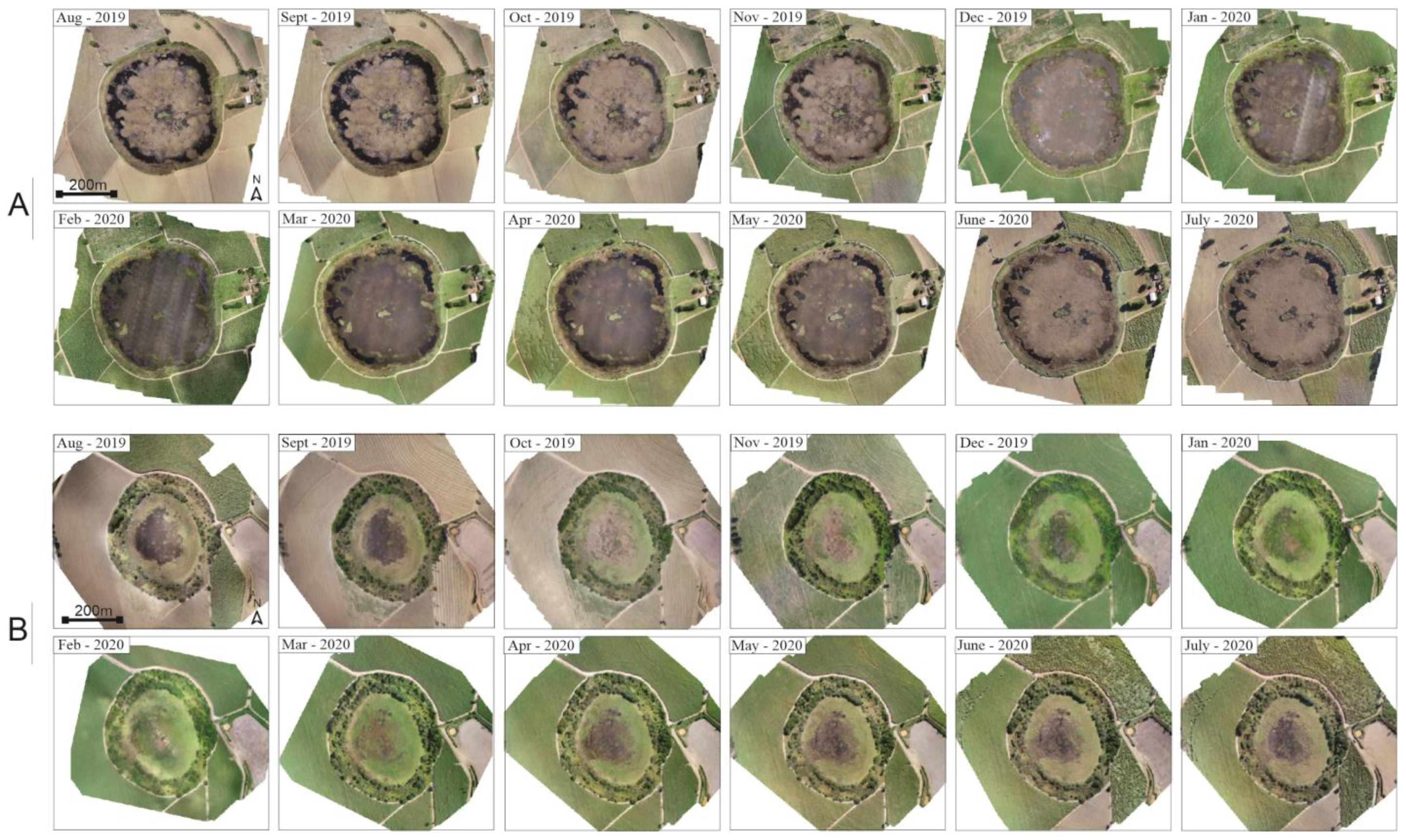
- August 2019–October 2019 and March 2019–July 2020: the decreased water level is associated with a retraction in the flooded borders (darkened portions) of orthomosaics, presenting ET > P. Although March shows positive values of water balance, the orthomosaics reveal a decrease in the amount of surface water in the wetlands;
- November 2019–February 2020: the water level rose, and the edges of the wetland expanded. Another imaging factor that indirectly indicates the rise of water level is the greater reflection of sunlight perceptible in the images of the period. The highest WB values and the highest water reflection in orthomosaics occur in the same months (January, February 2020), with P < ET. February is the month with the greater cumulative positive WB.For wetland B, it is also possible to integrate water-balance and orthomosaics into two distinct periods:
- August 2019–October 2019 and March 2019–July 2020: decrease in water level, reaching its minimum value in October 2019. The dominance of green color inside wetland area represents an increase of vegetation cover, ET > P;
- November 2019–July 2020: increase in water level. However, from December 2019 to February 2020, the area reached a water level that remained relatively stable, not presenting a sharp rise as suggested by the remarkable increase between January and February 2020 precipitation. Between March and July 2020 (dry period), unlike wetland A, wetland B presents an increase in water levels, despite the negative values in the WB, indicating a unique pattern of the wetland. P < ET. Two phenomena can occur simultaneously and explain this increase in pixels classified as water. The first is that the vegetation that dominates the wetland during the dry season is not resistant to moisture, so it is gradually suppressed during the flooding months, making the water more visible. The second is that during periods of drought, the wetland experiences less disturbance, which causes greater sedimentation of suspended particles, making the color more similar to that used in the supervised classification of water [74].
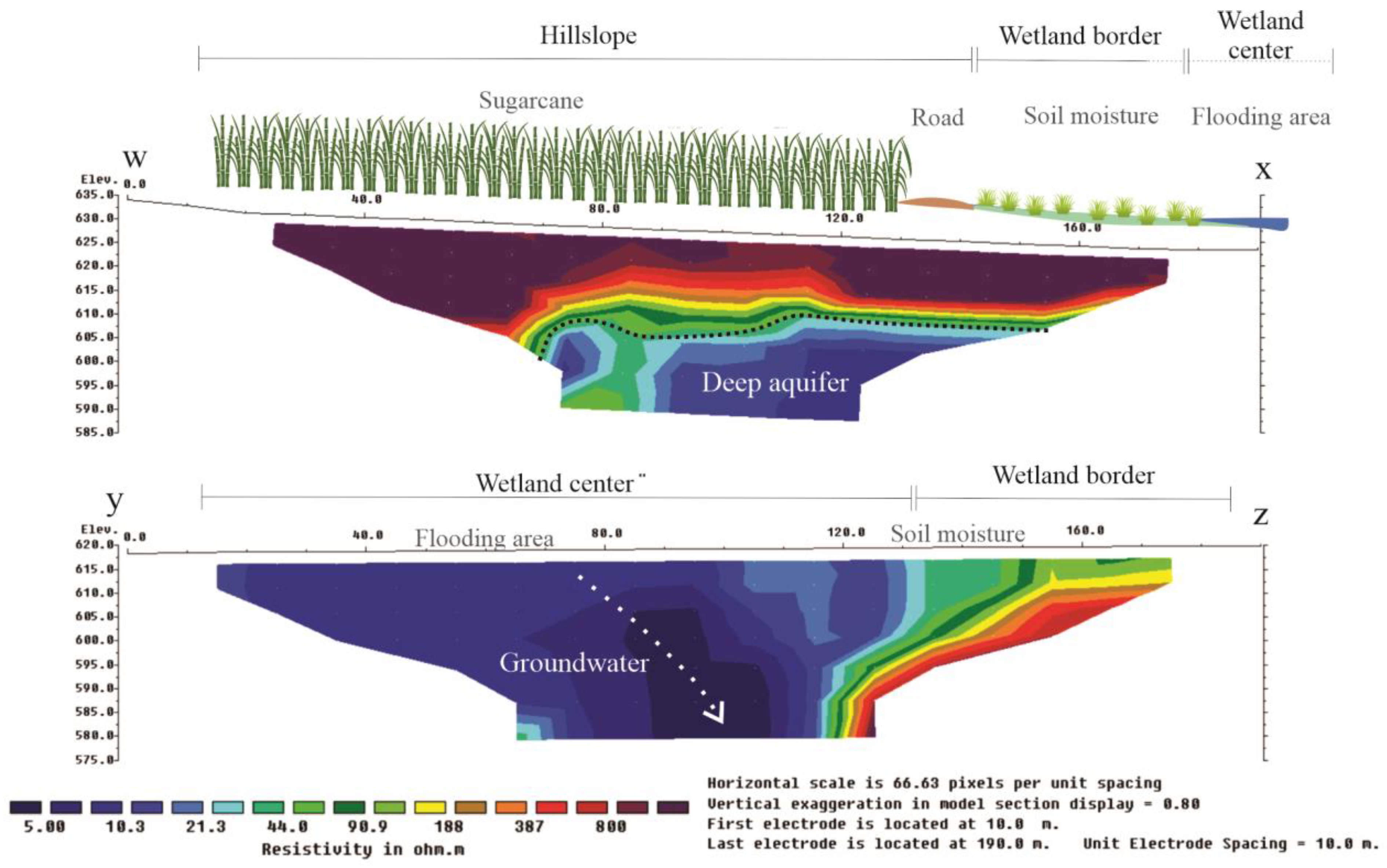
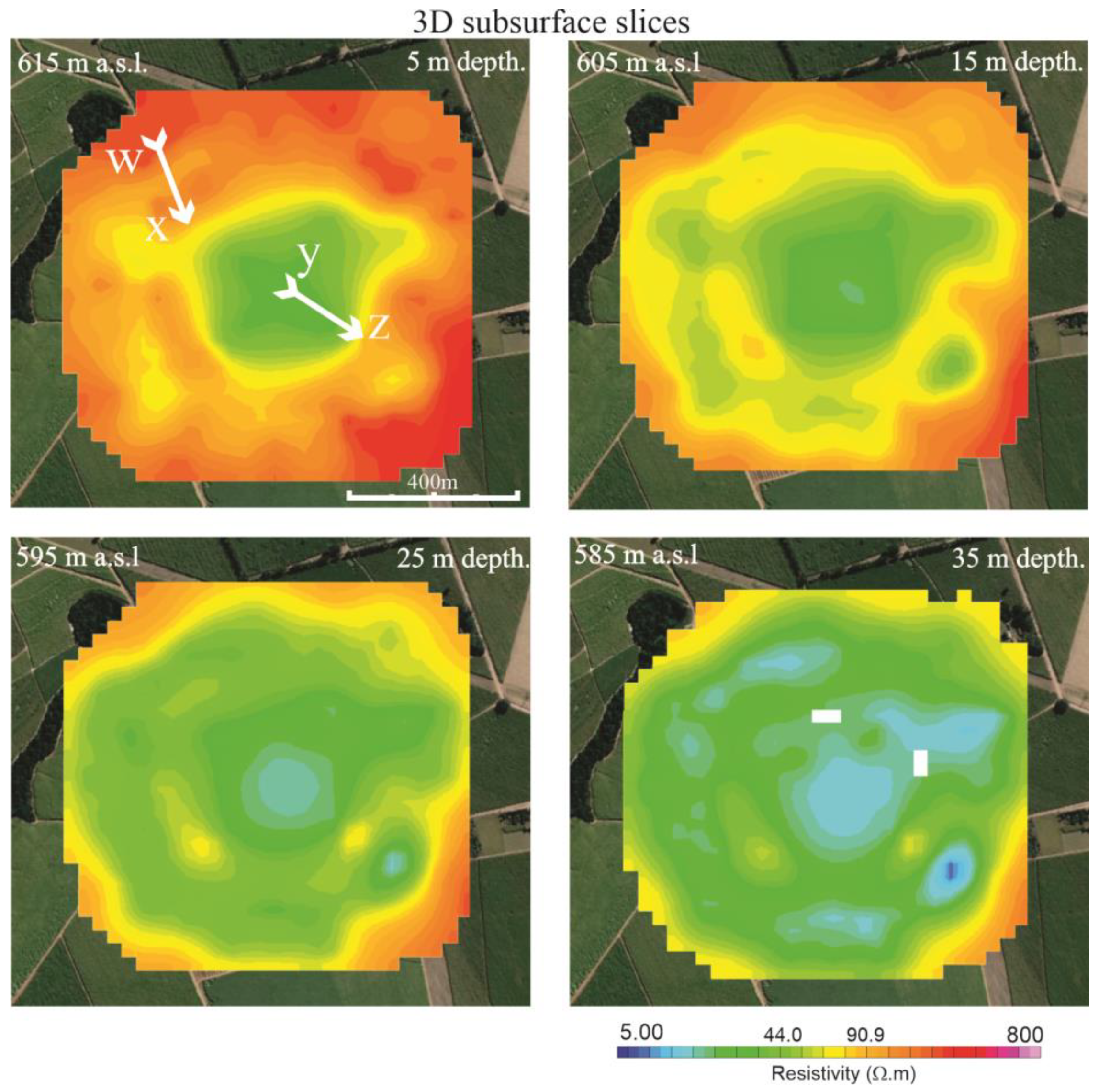
3.4. ERT Subsurface Imaging: 2D Profiles and 3D Slices
4. Discussion
5. Conclusions
Author Contributions
Funding
Data Availability Statement
Acknowledgments
Conflicts of Interest
References
- Moorkamp, M.; Lelièvre, P.G.; Linde, N.; Khan, A. Integrated imaging of the Earth. Theory and Applications; American Geophysical Union: Hoboken, NJ, USA; John Wiley and Sons: Hoboken, NJ, USA, 2016. [Google Scholar]
- Mousa, Y.A.; Hasan, A.F.; Helmholz, P. Spatio-Temporal Analysis of Sawa Lake’s Physical Parameters between (1985–2020) and Drought Investigations Using Landsat Imageries. Remote Sens. 2022, 14, 1831. [Google Scholar] [CrossRef]
- Mitsch, W.J.; Gosselink, J.G. The value of wetlands: Importance of scale and landscape setting. Ecol. Econ. 2000, 35, 25–33. [Google Scholar] [CrossRef]
- Rebelo, L.M.; Finlayson, C.M.; Nagabhatla, N. Remote sensing and GIS for wetland inventory, mapping and change analysis. J. Environ. Manag. 2009, 90, 2144–2153. [Google Scholar] [CrossRef] [PubMed]
- Neto, S. Water governance in an urban age. Util. Policy 2016, 43, 32–41. [Google Scholar] [CrossRef]
- Euliss, N.H.; Mushet, D.M. Impacts of water development on aquatic macroinvertebrates, amphibians, and plants in wetlands of a semi-arid landscape. Aquat. Ecosyst. Health 2004, 7, 73–84. [Google Scholar] [CrossRef]
- Melton, J.R.; Wania, R.; Hodson, E.L.; Poulter, B.; Ringeval, B.; Spahni, R.; Kaplan, J.O. Present state of global wetland extent and wetland methane modelling: Conclusions from a model inter-comparison project (WETCHIMP). Biogeosciences 2013, 10, 753–788. [Google Scholar] [CrossRef]
- Russi, D.; Ten Brink, P.; Farmer, A.; Badura, T.; Coates, D.; Förster, J.; Kumar, R.; Davidson, N. The economics of ecosystems and biodiversity for water and wetlands. IEEP Lond. Bruss. 2013, 78, 118. [Google Scholar]
- Ozesmi, S.L.; Bauer, M.E. Satellite remote sensing of wetlands. Wetl. Ecol. Manag. 2002, 10, 381–402. [Google Scholar] [CrossRef]
- Guo, M.; Li, J.; Sheng, C.; Xu, J.; Wu, L. A Review of Wetland Remote Sensing. Sensors 2017, 17, 777. [Google Scholar] [CrossRef]
- Reif, M.; Frohn, R.C.; Lane, C.R.; Autrey, B. Mapping Isolated Wetlands in a Karst Landscape: GIS and Remote Sensing Methods. GIScience Remote Sens. 2009, 46, 187–211. [Google Scholar] [CrossRef]
- Kandus, P.; Minotti, P.G.; Morandeira, N.S.; Grimson, R.; Trilla, G.G.; González, E.B.; Martín, L.S.; Gayol, M.P. Remote sensing of wetlands in South America: Status and challenges. Int. J. Remote Sens. 2018, 39, 993–1016. [Google Scholar] [CrossRef]
- Hakimdavar, R.; Hubbard, A.; Policelli, F.; Pickens, A.; Hansen, M.; Fatoyinbo, T.; Lagomasino, D.; Pahlevan, N.; Unninayar, S.; Kavvada, A. Monitoring water-related ecosystems with earth observation data in support of Sustainable Development Goal (SDG) 6 reporting. Remote Sens. 2020, 12, 1634. [Google Scholar] [CrossRef]
- Chabot, D.; Hodgson, A.J.; Hodgson, J.C.; Anderson, K. ‘Drone’: Technically correct, popularly accepted, socially acceptable: Different fields use different terms, but by changing its title, this journal is advocating for the discontinuation of ‘unmanned’ and recognition of ‘drone’ as an umbrella term for all robotic vehicles. Drone Syst. Appl. 2022, 10, 399–405. [Google Scholar]
- Debell, L.; Anderson, K.; Brazier, R.; King, N.; Jones, L. Water resource management at catchment scales using lightweight UAVs: Current capabilities and future perspectives. J. Unmanned Veh. Syst. 2016, 4, 7–30. [Google Scholar] [CrossRef]
- Chamoso, P.; González-Briones, A.; Rivas, A.; De Mata, F.B.; Corchado, J.M. The Use of Drones in Spain: Towards a Platform for Controlling UAVs in Urban Environments. Sensors 2018, 18, 1416. [Google Scholar] [CrossRef]
- Ledź, S.; Ewertowski, M.; Piekarczyk, J. Applications of unmanned aerial vehicle (UAV) surveys and Structure from Motion photogrammetry in glacial and periglacial geomorphology. Geomorphology 2021, 378, 107620. [Google Scholar]
- Golden, H.E.; Creed, I.F.; Ali, G.; Basu, N.B.; Neff, B.P.; Rains, M.C.; McLaughlin, D.L.; Alexander, L.C.; Ameli, A.A.; Christensen, J.R.; et al. Integrating geographically isolated wetlands into land management decisions. Front. Ecol. Environ. 2017, 15, 319–327. [Google Scholar] [CrossRef] [PubMed]
- Rains, M.; Leibowitz, S.G.; Cohen, M.J.; Creed, I.F.; Golden, H.E.; Jawitz, J.W.; Kalla, P.; Lane, C.R.; Lang, M.W.; McLaughlin, D.L. Geographically isolated wetlands are part of the hydrological landscape. Hydrol. Process. 2016, 30, 153–160. [Google Scholar] [CrossRef]
- Li, N.; Zhou, D.; Duan, F.; Wang, S.; Cui, Y. Application of unmanned airship image system and processing techniques for identifying of fresh water wetlands at a community scale. In Proceedings of the 2010 18th International Conference on Geoinformatics, Beijing, China, 18–20 July 2010; IEEE: Piscataway, NJ, USA; pp. 1–5. [Google Scholar] [CrossRef]
- Ouédraogo, M.M.; Degré, A.; Debouche, C.; Lisein, J. The evaluation of unmanned aerial system-based photogrammetry and terrestrial laser scanning to generate DEMs of agricultural watersheds. Geomorphology 2014, 214, 339–355. [Google Scholar] [CrossRef]
- Ishiguro, S.; Yamano, H.; Oguma, H. Evaluation of DSMs generated from multi-temporal aerial photographs using emerging structure from motion–multi-view stereo technology. Geomorphology 2016, 268, 64–71. [Google Scholar] [CrossRef]
- Iizuka, K.; Itoh, M.; Shiodera, S.; Matsubara, T.; Dohar, M.; Watanabe, K. Advantages of unmanned aerial vehicle (UAV) photogrammetry for landscape analysis compared with satellite data: A case study of postmining sites in Indonesia. Cogent Geosci. 2018, 4, 1498180. [Google Scholar] [CrossRef]
- James, M.R.; Robson, S. Straightforward reconstruction of 3D surfaces and topography with a camera: Accuracy and geoscience application. J. Geophys. Res. Earth Surf. 2012, 117, 03017. [Google Scholar] [CrossRef]
- Westoby, M.; Brasington, J.; Glasser, N.F.; Hambrey, M.J.; Reynolds, J.M. ‘Structure-from-Motion’ photogrammetry: A low-cost, effective tool for geoscience applications. Geomorphology 2012, 179, 300–314. [Google Scholar] [CrossRef]
- Fonstad, M.A.; Dietrich, J.T.; Courville, B.C.; Jensen, J.L.; Carbonneau, P.E. Topographic structure from motion: A new development in photogrammetric measurement. Earth Surf. Process. Landf. 2013, 38, 421–430. [Google Scholar] [CrossRef]
- Rubin, Y.; Hubbard, S.J. Hydrogeophysics; Springer: Dordrecht, The Netherlands, 2006. [Google Scholar]
- Moreira, C.A.; Rosolen, V.; Furlan, L.M.; Bovi, R.C.; Masquelin, H. Hydraulic conductivity and geophysics (ERT) to assess the aquifer recharge capacity of an inland wetland in the Brazilian Savanna. Environ. Chall. 2021, 5, 100274. [Google Scholar] [CrossRef]
- Lin, H.; Hopmans, J.W.; Richter, D.D. Interdisciplinary Sciences in a Global Network of Critical Zone Observatories. Vadose Zone J. 2011, 10, 781–785. [Google Scholar] [CrossRef]
- Linde, N.; Doetsch, J. Joint Inversion in Hydrogeophysics and Near-Surface Geophysics. In Integrated Imaging of the Earth. Theory and Applications; Moorkamp, M., Lelièvre, P.G., Linde, N., Khan, A., Eds.; American Geophysical Union: Hoboken, NJ, USA, 2016; pp. 119–135. [Google Scholar]
- Papastergiadou, E.S.; Retalis, A.; Apostolakis, A.; Georgiadis, T. Environmental Monitoring of Spatio-temporal Changes Using Remote Sensing and GIS in a Mediterranean Wetland of Northern Greece. Water Resour. Manag. 2008, 22, 579–594. [Google Scholar] [CrossRef]
- Haidary, A.; Amiri, B.J.; Adamowski, J.; Fohrer, N.; Nakane, K. Assessing the Impacts of Four Land Use Types on the Water Quality of Wetlands in Japan. Water Resour. Manag. 2013, 27, 2217–2229. [Google Scholar] [CrossRef]
- Ricaurte, L.F.; Olaya-Rodríguez, M.H.; Cepeda-Valencia, J.; Lara, D.; Arroyave-Suárez, J.; Finlayson, C.M.; Palomo, I. Future impacts of drivers of change on wetland ecosystem services in Colombia. Glob. Environ. Chang. 2017, 44, 158–169. [Google Scholar] [CrossRef]
- Mitsch, W.J.; Nahlik, A.; Wolski, P.; Bernal, B.; Zhang, L.; Ramberg, L. Tropical wetlands: Seasonal hydrologic pulsing, carbon sequestration, and methane emissions. Wetl. Ecol. Manag. 2009, 18, 573–586. [Google Scholar] [CrossRef]
- Cowood, A.L.; Young, J.; Dowling, T.I.; Moore, C.L.; Muller, R.; MacKenzie, J.; Littleboy, M.; Nicholson, A.T. Assessing wetland climate change vulnerability for wetland management decision support using the hydrogeological landscape framework: Application in the Australian Capital Territory. Mar. Freshw. Res. 2010, 70, 225. [Google Scholar] [CrossRef]
- Krasnostein, A.L.; Oldham, C. Predicting wetland water storage. Water Resour. Res. 2004, 40. [Google Scholar] [CrossRef]
- Zhang, G.; Bai, J.; Xi, M.; Zhao, Q.; Lu, Q.; Jia, J. Soil quality assessment of coastal wetlands in the Yellow River Delta of China based on the minimum data set. Ecol. Indic. 2016, 66, 458–466. [Google Scholar] [CrossRef]
- Sano, E.E.; Rosa, R.; Brito, J.L.S.; Ferreira, L.G. Land cover mapping of the tropical savanna region in Brazil. Environ. Monit. Assess. 2010, 166, 113–124. [Google Scholar] [CrossRef] [PubMed]
- Martinelli, L.A.; Filoso, S. Expansion of Sugarcane Ethanol Production in Brazil: Environmental and Social Challenges. Ecol. Appl. 2008, 18, 885–898. [Google Scholar] [CrossRef]
- Ussami, K.A.; Guilhoto, J.J.M. Economic and water dependence among regions: The case of Alto Tiete, Sao Paulo State, Brazil. Economia 2018, 19, 350–376. [Google Scholar] [CrossRef]
- Almeida, F.F.M. Geological foundations of São Paulo relief. São Paulo: Geographic and Geological Institute. Geol. State São Paulo 1964, 41, 167–263. [Google Scholar]
- Koeppen, W. Climatologia: Con un Estudio de Los Climas de la Tierra. Fondo de Cultura Econômica: Ciudad de Mexico, Mexic, 1948; p. 479. [Google Scholar]
- Cepagri. Clima dos Municípios Paulistas. Available online: http://www.cpa.unicamp.br (accessed on 28 July 2020).
- Modelo Digital de Elevação. Estado de São Paulo. Available online: Infraestruturameioambiente.sp.gov.br (accessed on 15 June 2020).
- Junqueira, D.A. Principles of the Environmental Governance in Water Resource Management Focusing on Wetlands at Depressão Periférica Paulista. Ph.D. Thesis, São Paulo State Universtiy, São Paulo, Brazil, 2020. [Google Scholar]
- Furlan, L.M.; Moreira, C.A.; de Alencar, P.G.; Rosolen, V. Environmental monitoring and hydrological simulations of a natural wetland based on high-resolution unmanned aerial vehicle data (Paulista Peripheral Depression, Brazil). Environ. Chall. 2021, 4, 100146. [Google Scholar] [CrossRef]
- Instituto Nacional de Pesquisas Espaciais. Available online: http://www.dgi.inpe.br/catalogo/ (accessed on 17 June 2020).
- USGS Earth Explorer. Available online: https://earthexplorer.usgs.gov (accessed on 20 June 2020).
- Lang, M.W.; Purkis, S.; Klemas, V.V.; Tiner, R.W. 25 Promising Developments and Future Challenges for Remote Sensing of Wetlands; Taylor and Francis: Boca Raton, FL, USA, 2015. [Google Scholar]
- Jensen, J.R. Remote Sensing of the Environment: An Earth Resource Perspective 2/e; Pearson Education: New Delhi, India, 2009. [Google Scholar]
- Li, Z.; Guo, X. Non-photosynthetic vegetation biomass estimation in semiarid Canadian mixed grasslands using ground hyperspectral data, Landsat 8 OLI, and Sentinel-2 images. Int. J. Remote Sens. 2018, 39, 6893–6913. [Google Scholar] [CrossRef]
- Taddeo, S.; Dronova, I.; Depsky, N. Spectral vegetation indices of wetland greenness: Responses to vegetation structure, composition, and spatial distribution. Remote Sens. Environ. 2019, 234, 111467. [Google Scholar] [CrossRef]
- Xu, H.; Gao, P. Custom image processing capabilities in ARCGIS. The International Archives of the Photogrammetry. Remote Sens. Spat. Inf. Sci. 2008, 37, 263–266. [Google Scholar]
- Hu, T.; Liu, J.; Zheng, G.; Zhang, D.; Huang, K. Evaluation of historical and future wetland degradation using remote sensing imagery and land use modeling. Land Degrad. Dev. 2020, 31, 65–80. [Google Scholar] [CrossRef]
- DJI. Phantom 4PRO. Available online: https://www.dji.com/br/phantom-4-pro (accessed on 30 November 2022).
- PIX4D. Available online: https://www.pix4d.com/ (accessed on 30 November 2022).
- Dandois, J.P.; Olano, M.; Ellis, E.C. Optimal Altitude, Overlap, and Weather Conditions for Computer Vision UAV Estimates of Forest Structure. Remote Sens. 2015, 7, 13895–13920. [Google Scholar] [CrossRef]
- D’Oleire-Oltmanns, S.; Marzolff, I.; Peter, K.D.; Ries, J.B. Unmanned Aerial Vehicle (UAV) for Monitoring Soil Erosion in Morocco. Remote Sens. 2012, 4, 3390–3416. [Google Scholar] [CrossRef]
- Gomez, C.; Hayakawa, Y.; Obanawa, H. A study of Japanese landscapes using structure from motion derived DSMs and DEMs based on historical aerial photographs: New opportunities for vegetation monitoring and diachronic geomorphology. Geomorphology 2015, 242, 11–20. [Google Scholar] [CrossRef]
- Agisoft Metashape Professional Software, Version 1.6.3. Available online: https://www.agisoft.com (accessed on 30 November 2022).
- Collischonn, C.; de Lima, E.M.; Ruiz, L.F.C.; Araujo, T.D.; Matsuoka, M.T. Posicionamento GNSS: Comparação entre coordenadas oficiais de estações da RBMC e as obtidas por PPP e posicionamento relativo e ajustamento. In Simpósio Brasileiro de Sensoriamento Remoto—SBSR.; INPE: João Pessoa, Brazil, 2015. [Google Scholar]
- Sales, J.C.; Bueno, G.T.; Rosolen, V.; Ferreira, M.E.; Furlan, L.M. The structure of an earth-mound field of the Brazilian Savanna. Geomorphology 2021, 386, 107752. [Google Scholar] [CrossRef]
- CEAPLA. Available online: https://igce.rc.unesp.br/#!/ceapla (accessed on 15 October 2022).
- Fries, A.; Silva, K.; Pucha-Cofrep, F.; Oñate-Valdivieso, F.; Ochoa-Cueva, P. Water Balance and Soil Moisture Deficit of Different Vegetation Units under Semiarid Conditions in the Andes of Southern Ecuador. Climate 2020, 8, 30. [Google Scholar] [CrossRef]
- Kearey, P.; Brooks, M.; Hill, I. An introduction to geophysical exploration. In Tradução de Maria Cristina Moreira Coelho, 1st ed; Oficina de Textos: São Paulo, Brazil, 2002. (In Portuguese) [Google Scholar]
- Milson, J. Field Geophysics; John Wiley & Sons: Sussex, UK, 2003. [Google Scholar]
- Mussett, A.E.; Khan, M.A. Looking into the Earth: An Introduction to Geological Geophysics. Cambridge University Press: London, England, 2000. [Google Scholar]
- Terrameter, L.S. Instruction Manual; ABEM Instrument: Sundbyberg, Sweden, 2012. [Google Scholar]
- Casagrande, M.F.S.; Furlan, L.M.; Moreira, C.A.; Rosa, F.T.G.; Rosolen, V. Non-invasive methods in the identification of hydrological ecosystem services of a tropical isolated wetland (Brazilian study case). Environ. Chall. 2021, 5, 100233. [Google Scholar] [CrossRef]
- Rosa, F.T.G.; Moreira, C.A.; Rosolen, V.; Casagrande, M.; Bovi, R.C.; Furlan, L.M.; dos Santos, S.F. Detection of Aquifer Recharge Zones in Isolated Wetlands: Comparative Analysis Among Electrical Resistivity Tomography Arrays. Pure Appl. Geophys. 2022, 179, 1275–1294. [Google Scholar] [CrossRef]
- Geotomo Software. Geoelectrical Imaging 2-D & 3D; Geotomo: Penang, Malaysia, 2003; 129p. [Google Scholar]
- Chulès, J.P.; Delfiner, P. Geostatistics—Modeling Spatial Uncertainty, 2nd ed.; Wiley: Hoboken, NJ, USA, 2012. [Google Scholar]
- Oasis Montaj. Available online: https://www.seequent.com/ (accessed on 20 November 2022).
- Mahdavi, S.; Salehi, B.; Granger, J.; Amani, M.; Brisco, B.; Huang, W. Remote sensing for wetland classification: A comprehensive review. GIScience Remote Sens. 2018, 55, 623–658. [Google Scholar] [CrossRef]
- Peng, H.; Xia, H.; Shi, Q.; Chen, H.; Chu, N.; Liang, J.; Gao, Z. Monitoring spatial and temporal dynamics of wetland vegetation and their response to hydrological conditions in a large seasonal lake with time series Landsat data. Ecol. Indic. 2022, 142, 109283. [Google Scholar] [CrossRef]
- Walton, C.R.; Zak, D.; Audet, J.; Petersen, R.J.; Lange, J.; Oehmke, C.; Wichtmann, W.; Kreyling, J.; Grygoruk, M.; Jabłońska, E.; et al. Wetland buffer zones for nitrogen and phosphorus retention: Impacts of soil type, hydrology and vegetation. Sci. Total Environ. 2020, 727, 138709. [Google Scholar] [CrossRef] [PubMed]
- Jarvis, N.J.; Moeys, J.; Koestel, J.; Hollis, J.M.; Lin, H. Preferential Flow in a Pedological Perspective; Hydropedology; Academic Press: Waltham, MA, USA, 2012; pp. 75–120. [Google Scholar]
- Frei, S.; Lischeid, G.; Fleckenstein, J. Effects of micro-topography on surface–subsurface exchange and runoff generation in a virtual riparian wetland—A modeling study. Adv. Water Resour. 2010, 33, 1388–1401. [Google Scholar] [CrossRef]
- Lee, S.; McCarty, G.W.; Moglen, G.E.; Lang, M.W.; Jones, C.N.; Palmer, M.; Yeo, I.-Y.; Anderson, M.; Sadeghi, A.M.; Rabenhorst, M.C. Seasonal drivers of geographically isolated wetland hydrology in a low-gradient, Coastal Plain landscape. J. Hydrol. 2020, 583, 124608. [Google Scholar] [CrossRef]
- Kite, G. Land Surface Parameterizations of Gcms and Macroscale Hydrological Models. JAWRA J. Am. Water Resour. Assoc. 1998, 34, 1247–1254. [Google Scholar] [CrossRef]
- Coral, A.C.; Tommaselli, J.T.G.; Leal, A.C. Cálculo de balance hídrico usando modelamiento de datos espaciales: Estudio aplicado a la cuenca del río Buena Vista, Ecuador. Formação 2015, 1. [Google Scholar]
- Tiner, R.W. Geographically isolated wetlands of the United States. Wetlands 2003, 23, 494–516. [Google Scholar] [CrossRef]
- Guo, Y.; Liao, H.-L.; Boughton, E.H.; Martens-Habbena, W.; Qiu, J. Effects of land-use intensity, grazing and fire disturbances on soil bacterial and fungal communities in subtropical wetlands. Agric. Ecosyst. Environ. 2023, 345, 108314. [Google Scholar] [CrossRef]
- Boughton, E.H.; Quintana-Ascencio, P.F.; Bohlen, P.J.; Fauth, J.E.; Jenkins, D.G. Interactive effects of pasture management intensity, release from grazing and prescribed fire on forty subtropical wetland plant assemblages. J. Appl. Ecol. 2016, 53, 159–170. [Google Scholar] [CrossRef]
- Yan, W.; Wang, Y.; Chaudhary, P.; Ju, P.; Zhu, Q.; Kang, X.; Chen, H.; He, Y. Effects of climate change and human activities on net primary production of wetlands on the Zoige Plateau from 1990 to 2015. Glob. Ecol. Conserv. 2020, 35, e02052. [Google Scholar] [CrossRef]
- Conciani, D.E.; dos Santos, L.P.; Silva, T.S.F.; Durigan, G.; Alvarado, S.T. Human-climate interactions shape fire regimes in the Cerrado of São Paulo state, Brazil. J. Nat. Conserv. 2021, 61, 126006. [Google Scholar] [CrossRef]
- da Silva, G.J.; Berg, E.C.; Calijuri, M.L.; dos Santos, V.J.; Lorentz, J.F.; Alves, S.D.C. Aptitude of areas planned for sugarcane cultivation expansion in the state of São Paulo, Brazil: A study based on climate change effects. Agric. Ecosyst. Environ. 2021, 305, 107164. [Google Scholar] [CrossRef]
- Blake, W.H.; Kelly, C.; Wynants, M.; Patrick, A.; Lewin, S.; Lawson, J.; Nasolwa, E.; Page, A.; Nasseri, M.; Marks, C.; et al. Integrating land-water-people connectivity concepts across disciplines for co-design of soil erosion solutions. Land Degrad. Dev. 2021, 32, 3415–3430. [Google Scholar] [CrossRef]
- Vepraskas, M.; Lindbo, D.; Lin, H. Redoximorphic Features as Related to Soil Hydrology and Hydric Soils; Hydropedology; Academic Press: Waltham, MA, USA, 2012; pp. 143–172. [Google Scholar] [CrossRef]
- Espinar, J.L.; Clemente, L. The impact of vertic soil cracks on submerged macrophyte diaspore bank depth distribution in Mediterranean temporary wetlands. Aquat. Bot. 2007, 87, 325–328. [Google Scholar] [CrossRef]
- Evenson, G.R.; Golden, H.E.; Lane, C.R.; McLaughlin, D.L.; D'Amico, E. Depressional wetlands affect watershed hydrological, biogeochemical, and ecological functions. Ecol. Appl. 2018, 28, 953–966. [Google Scholar] [CrossRef] [PubMed]
- Euliss, N.H.; Mushet, D.M. Water-level fluctuation in wetlands as a function of landscape condition in the prairie pothole region. Wetlands 1996, 16, 587–593. [Google Scholar] [CrossRef]
- Trettin, C.C.; Kolka, R.K.; Marsh, A.S.; Bansal, S.; Lilleskov, E.A.; Megonigal, P.; Stelk, M.J.; Lockaby, G.; D’Amore, D.V.; Mac-Kenzie, R.A.; et al. Wetland and hydric soil. In Forest and Rangeland Soils of the United States Under Changing Conditions; Pouyat, R.V., Page-Dumroese, D.S., Patel-Weynand, T., Geiser, L.H., Eds.; Springer: Cham, Switzerland, 2020; pp. 99–126. [Google Scholar]
- Chen, L.; Jin, Z.; Michishita, R.; Cai, J.; Yue, T.; Chen, B.; Xu, B. Dynamic monitoring of wetland cover changes using time-series remote sensing imagery. Ecol. Inform. 2014, 24, 17–26. [Google Scholar] [CrossRef]
- Cohen, M.J.; Creed, I.F.; Alexander, L.; Basu, N.B.; Calhoun, A.J.K.; Craft, C.; D’Amico, E.; DeKeyser, E.; Fowler, L.; Golden, H.E.; et al. Do geographically isolated wetlands influence landscape functions? Proc. Natl. Acad. Sci. USA 2016, 113, 1978–1986. [Google Scholar] [CrossRef]
- Winter, T.C. Hydrologic studies of wetlands in the Northern Prairies. In Northern Prairie Wetlands; van der Valk, A., Ed.; Iowa State University Press: Ames, IA, USA, 1989; pp. 16–54. [Google Scholar]


| Year | Season | Satellite | Sensor | Band Composition | Resolution |
|---|---|---|---|---|---|
| 1975 | Dry | Landsat 2 | MSS | 6(NIR)-7(NIR)-5(R) | 80 m |
| 1984 | Dry | Landsat 5 | TM | 4(NIR)-5(SWIR 1)-3(R) | 30 m |
| 1992 | Dry | Landsat 5 | TM | 4(NIR)-5(SWIR 1)-3(R) | 30 m |
| 2000 | Dry | Landsat 7 | ETM+ | 4(NIR)-5(SWIR 1)-3(R) + 8 (PAN) | 30 m (15 m) |
| 2010 | Dry | Landsat 5 | TM | 4(NIR)-5(SWIR 1)-3(R) | 30 m |
| 2020 | Wet | CBERS-04A | WPM | 3(R)-4(NIR)-2(G) + 0 (PAN) | 8 m (2 m) |
| October 2019 | February 2020 | |||
|---|---|---|---|---|
| Compartment | Area (m2) | Compartment | Area (m2) | |
| Wetland A | A1dry | 57,259 | A1wet | 42,316 |
| A2dry | 21,306 | A2wet | 130,339 | |
| A3dry | 94,089 | |||
| Wetland B | B1dry | 34,134 | B1wet | 34,134 |
| B2dry | 31,558 | B2wet | 10,200 | |
| B3wet | 21,358 | |||
| Month | P (mm) | ET (mm) | WB (mm) | |
|---|---|---|---|---|
| Period 1 | August-19 | 13.8 | 95.1 | 81.3 |
| September-19 | 56 | 112.08 | 56.8 | |
| October-19 | 126.4 | 138.74 | 12.34 | |
| Period 2 | November-19 | 171.1 | 116.5 | 54.6 |
| December-19 | 151.5 | 112.11 | 39.39 | |
| January-20 | 175 | 114.28 | 60.72 | |
| February-20 | 315 | 83.19 | 231.81 | |
| Period 1 | March-20 | 128.4 | 114.19 | 14.21 |
| April-20 | 8.4 | 102.95 | 94.55 | |
| May-20 | 23.6 | 80.74 | 57.14 | |
| June-20 | 79.2 | 68.36 | 10.84 | |
| July-20 | 8.2 | 80.55 | 73.35 |
Disclaimer/Publisher’s Note: The statements, opinions and data contained in all publications are solely those of the individual author(s) and contributor(s) and not of MDPI and/or the editor(s). MDPI and/or the editor(s) disclaim responsibility for any injury to people or property resulting from any ideas, methods, instructions or products referred to in the content. |
© 2023 by the authors. Licensee MDPI, Basel, Switzerland. This article is an open access article distributed under the terms and conditions of the Creative Commons Attribution (CC BY) license (https://creativecommons.org/licenses/by/4.0/).
Share and Cite
Furlan, L.M.; Ferreira, M.E.; Moreira, C.A.; de Alencar, P.G.; Casagrande, M.F.S.; Rosolen, V. Satellite, UAV, and Geophysical Data to Identify Surface and Subsurface Hydrodynamics of Geographically Isolated Wetlands: Understanding an Undervalued Ecosystem at the Atlantic Forest-Cerrado Interface of Brazil. Remote Sens. 2023, 15, 1870. https://doi.org/10.3390/rs15071870
Furlan LM, Ferreira ME, Moreira CA, de Alencar PG, Casagrande MFS, Rosolen V. Satellite, UAV, and Geophysical Data to Identify Surface and Subsurface Hydrodynamics of Geographically Isolated Wetlands: Understanding an Undervalued Ecosystem at the Atlantic Forest-Cerrado Interface of Brazil. Remote Sensing. 2023; 15(7):1870. https://doi.org/10.3390/rs15071870
Chicago/Turabian StyleFurlan, Lucas Moreira, Manuel Eduardo Ferreira, César Augusto Moreira, Paulo Guilherme de Alencar, Matheus Felipe Stanfoca Casagrande, and Vânia Rosolen. 2023. "Satellite, UAV, and Geophysical Data to Identify Surface and Subsurface Hydrodynamics of Geographically Isolated Wetlands: Understanding an Undervalued Ecosystem at the Atlantic Forest-Cerrado Interface of Brazil" Remote Sensing 15, no. 7: 1870. https://doi.org/10.3390/rs15071870
APA StyleFurlan, L. M., Ferreira, M. E., Moreira, C. A., de Alencar, P. G., Casagrande, M. F. S., & Rosolen, V. (2023). Satellite, UAV, and Geophysical Data to Identify Surface and Subsurface Hydrodynamics of Geographically Isolated Wetlands: Understanding an Undervalued Ecosystem at the Atlantic Forest-Cerrado Interface of Brazil. Remote Sensing, 15(7), 1870. https://doi.org/10.3390/rs15071870