
Woody Plant Encroachment in a Seasonal Tropical Savanna: Lessons about Classifiers and Accuracy from UAV Images
 , , , , and
Abstract
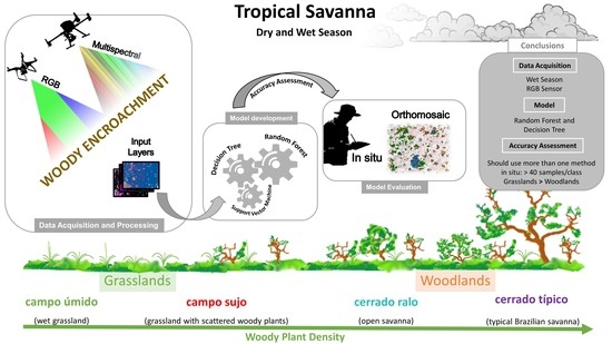
1. Introduction
2. Materials and Methods
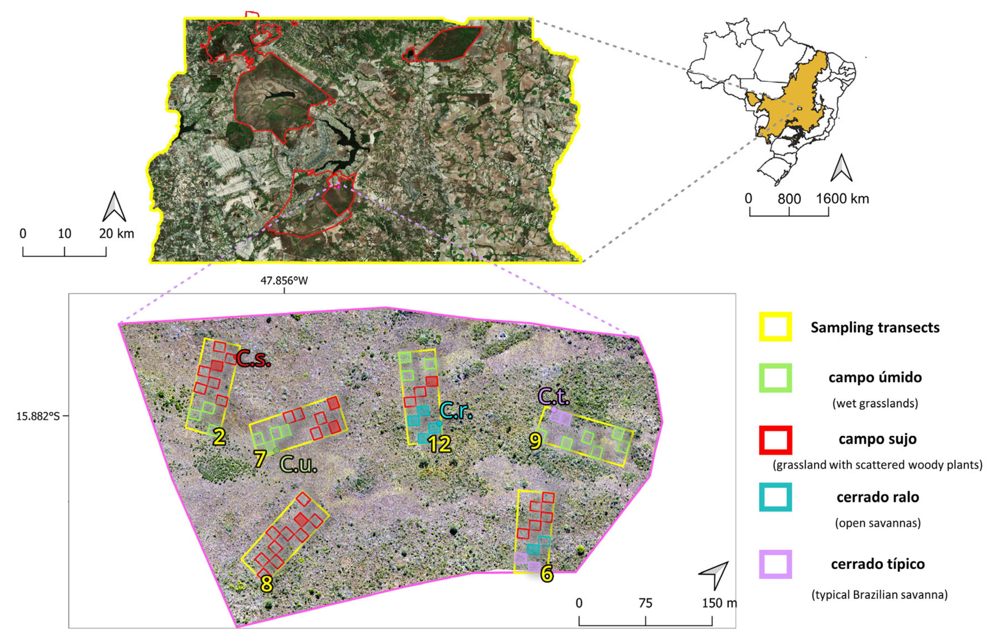
2.1. Study Area
2.2. Studied Species
2.3. Field Data Gathering and Digital Image Processing
2.4. Generation of Layers, Masks, and Metrics
2.5. Image Segmentation and Zonal Statistics
2.6. Object-Based Supervised Classification
2.7. Accuracy Assessment and In Situ Validation
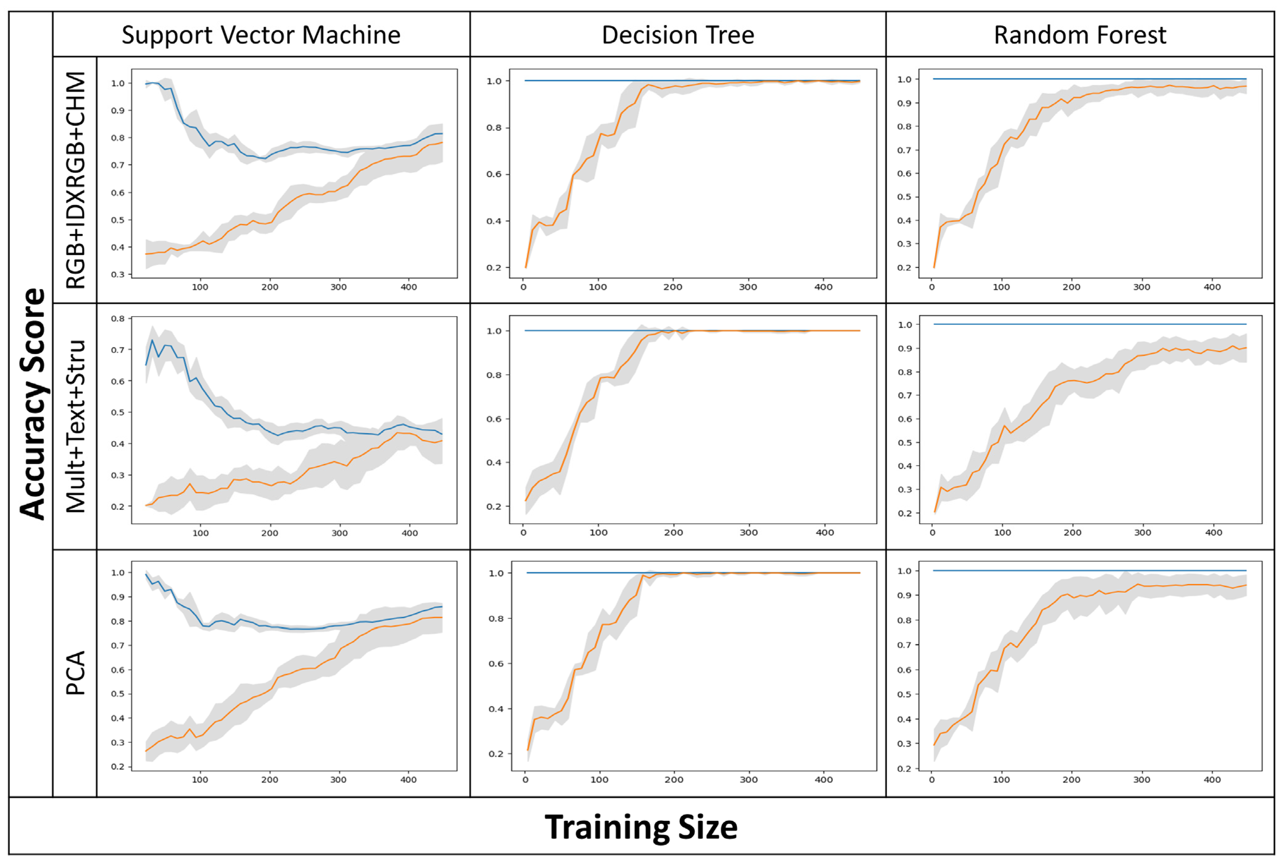
3. Results
3.1. Classifiers, Input Layers, and Climatic Seasons’ Accuracy Assessment
3.2. In Situ Validation and Cerrado Phytophysiognomy Accuracy Assessment
4. Discussion
4.1. Overall Accuracy Assessment and Model Validity
4.2. In Situ Validation
4.3. Evaluating In Situ Accuracy in Different Phytophysiognomies
5. Conclusions
Supplementary Materials
Author Contributions
Funding
Data Availability Statement
Acknowledgments
Conflicts of Interest
References
- Mack, R.N.; Simberloff, D.; Lonsdale, W.M.; Evans, H.; Clout, M.; Bazzaz, F.A. Biotic Invasions: Causes, Epidemiology, Global Consequences, and Control. Ecol. Appl. 2000, 10, 689–710. [Google Scholar] [CrossRef]
- Valéry, L.; Fritz, H.; Lefeuvre, J.-C.; Simberloff, D. In Search of a Real Definition of the Biological Invasion Phenomenon Itself. Biol. Invasions 2008, 10, 1345–1351. [Google Scholar] [CrossRef]
- Vitousek, P.M. Biological Invasions and Ecosystem Processes: Towards an Integration of Population Biology and Ecosystem Studies. Oikos 1990, 57, 7–13. [Google Scholar] [CrossRef]
- Richardson, D.M.; Pyšek, P.; Rejmánek, M.; Barbour, M.G.; Panetta, F.D.; West, C.J. Naturalization and Invasion of Alien Plants: Concepts and Definitions. Divers. Distrib. 2000, 6, 93–107. [Google Scholar] [CrossRef]
- Irini, S.; Xulin, G. Invasive and Native Woody Plant Encroachment: Definitions and Debates. J. Plant Sci. Phytopathol. 2022, 6, 84–86. [Google Scholar] [CrossRef]
- Eldridge, D.J.; Bowker, M.A.; Maestre, F.T.; Roger, E.; Reynolds, J.F.; Whitford, W.G. Impacts of Shrub Encroachment on Ecosystem Structure and Functioning: Towards a Global Synthesis. Ecol. Lett. 2011, 14, 709–722. [Google Scholar] [CrossRef]
- Archer, S.R.; Predick, K.I. An Ecosystem Services Perspective on Brush Management: Research Priorities for Competing Land-Use Objectives. J. Ecol. 2014, 102, 1394–1407. [Google Scholar] [CrossRef]
- Saintilan, N.; Rogers, K. Woody Plant Encroachment of Grasslands: A Comparison of Terrestrial and Wetland Settings. New Phytol. 2015, 205, 1062–1070. [Google Scholar] [CrossRef]
- Van Auken, O.W. Causes and Consequences of Woody Plant Encroachment into Western North American Grasslands. J. Environ. Manag. 2009, 90, 2931–2942. [Google Scholar] [CrossRef]
- Scholes, R.J.; Archer, S.R. Tree-Grass Interactions in Savannas. Annu. Rev. Ecol. Syst. 1997, 28, 517–544. [Google Scholar] [CrossRef]
- Bond, W.; Keeley, J. Fire as a Global ‘Herbivore’: The Ecology and Evolution of Flammable Ecosystems. Trends Ecol. Evol. 2005, 20, 387–394. [Google Scholar] [CrossRef] [PubMed]
- Huxman, T.E.; Wilcox, B.P.; Breshears, D.D.; Scott, R.L.; Snyder, K.A.; Small, E.E.; Hultine, K.; Pockman, W.T.; Jackson, R.B. Ecohydrological Implications of Woody Plant Encroachment. Ecology 2005, 86, 308–319. [Google Scholar] [CrossRef]
- O’Connor, T.G.; Puttick, J.R.; Hoffman, M.T. Bush Encroachment in Southern Africa: Changes and Causes. Afr. J. Range Forage Sci. 2014, 31, 67–88. [Google Scholar] [CrossRef]
- Puttick, J.R.; Hoffman, M.T.; Gambiza, J. The Influence of South Africa’s Post-Apartheid Land Reform Policies on Bush Encroachment and Range Condition: A Case Study of Fort Beaufort’s Municipal Commonage. Afr. J. Range Forage Sci. 2014, 31, 135–145. [Google Scholar] [CrossRef]
- Van Auken, O.W. Shrub Invasions of North American Semiarid Grasslands. Annu. Rev. Ecol. Syst. 2000, 31, 197–215. [Google Scholar] [CrossRef]
- Schlesinger, W.H.; Raikes, J.A.; Hartley, A.E.; Cross, A.F. On the Spatial Pattern of Soil Nutrients in Desert Ecosystems. Ecology 1996, 77, 364–374. [Google Scholar] [CrossRef]
- D’Odorico, P.; Caylor, K.; Okin, G.S.; Scanlon, T.M. On Soil Moisture–Vegetation Feedbacks and Their Possible Effects on the Dynamics of Dryland Ecosystems. J. Geophys. Res. Biogeosci. 2007, 112, G04010. [Google Scholar] [CrossRef]
- D’Odorico, P.; Fuentes, J.D.; Pockman, W.T.; Collins, S.L.; He, Y.; Medeiros, J.S.; DeWekker, S.; Litvak, M.E. Positive Feedback between Microclimate and Shrub Encroachment in the Northern Chihuahuan Desert. Ecosphere 2010, 1, 17. [Google Scholar] [CrossRef]
- Silva, F.H.B.; Arieira, J.; Parolin, P.; Cunha, C.N.; Junk, W.J. Shrub Encroachment Influences Herbaceous Communities in Flooded Grasslands of a Neotropical Savanna Wetland. Appl. Veg. Sci. 2016, 19, 391–400. [Google Scholar] [CrossRef]
- Siraj, K.G.; Abdella, G. Effects of Bush Encroachment on Plant Composition, Diversity and Carbon Stock in Borana Rangelands, Southern Ethiopia. Int. J. Biodivers. Conserv. 2018, 10, 230–245. [Google Scholar] [CrossRef]
- Gonçalves, R.V.S.; Cardoso, J.C.F.; Oliveira, P.E.; Oliveira, D.C. Changes in the Cerrado Vegetation Structure: Insights from More than Three Decades of Ecological Succession. Web Ecol. 2021, 21, 55–64. [Google Scholar] [CrossRef]
- Ribeiro, J.W.F.; Pilon, N.A.L.; Rossatto, D.R.; Durigan, G.; Kolb, R.M. The Distinct Roles of Water Table Depth and Soil Properties in Controlling Alternative Woodland-Grassland States in the Cerrado. Oecologia 2021, 195, 641–653. [Google Scholar] [CrossRef] [PubMed]
- Souza, G.F.; Ferreira, M.C.; Munhoz, C.B.R. Decrease in Species Richness and Diversity, and Encroachment in Cerrado Grasslands: A 20 Years Study. Appl. Veg. Sci. 2022, 25, e12668. [Google Scholar] [CrossRef]
- Ge, J.; Zou, C. Impacts of Woody Plant Encroachment on Regional Climate in the Southern Great Plains of the United States: Woody Encroachment and Climate. J. Geophys. Res. Atmos. 2013, 118, 9093–9104. [Google Scholar] [CrossRef]
- Honda, E.A.; Durigan, G. Woody Encroachment and Its Consequences on Hydrological Processes in the Savannah. Philos. Trans. R. Soc. B Biol. Sci. 2016, 371, 20150313. [Google Scholar] [CrossRef]
- Luvuno, L.; Biggs, R.; Stevens, N.; Esler, K. Woody Encroachment as a Social-Ecological Regime Shift. Sustainability 2018, 10, 2221. [Google Scholar] [CrossRef]
- Foxcroft, L.C.; Pyšek, P.; Richardson, D.M.; Genovesi, P. (Eds.) Plant Invasions in Protected Areas: Patterns, Problems and Challenges; Springer: Dordrecht, The Netherlands, 2013. [Google Scholar] [CrossRef]
- Morford, S.L.; Allred, B.W.; Twidwell, D.; Jones, M.O.; Maestas, J.D.; Naugle, D.E. Tree Invasions Threaten the Conservation Potential and Sustainability of U.S. Rangelands. J. Appl. Ecol. 2022, 59, 2971–2982. [Google Scholar] [CrossRef]
- Nackley, L.L.; West, A.G.; Skowno, A.L.; Bond, W.J. The Nebulous Ecology of Native Invasions. Trends Ecol. Evol. 2017, 32, 814–824. [Google Scholar] [CrossRef]
- Britz, M.; Ward, D. Dynamics of Woody Vegetation in a Semi-Arid Savanna, with a Focus on Bush Encroachment. Afr. J. Range Forage Sci. 2007, 24, 131–140. [Google Scholar] [CrossRef]
- Rohde, R.F.; Hoffman, M.T. The Historical Ecology of Namibian Rangelands: Vegetation Change since 1876 in Response to Local and Global Drivers. Sci. Total Environ. 2012, 416, 276–288. [Google Scholar] [CrossRef]
- Puttick, J.R.; Hoffman, M.T.; Gambiza, J. The Impact of Land Use on Woody Plant Cover and Species Composition on the Grahamstown Municipal Commonage: Implications for South Africa’s Land Reform Programme. Afr. J. Range Forage Sci. 2014, 31, 123–133. [Google Scholar] [CrossRef]
- Thompson, W.A.; Eldridge, D.J. Plant Cover and Composition in Relation to Density of Callitris glaucophylla (White Cypress Pine) along a Rainfall Gradient in Eastern Australia. Aust. J. Bot. 2005, 53, 545. [Google Scholar] [CrossRef]
- Tighe, M.; Reid, N.; Wilson, B.; Briggs, S.V. Invasive Native Scrub and Soil Condition in Semi-Arid South-Eastern Australia. Agric. Ecosyst. Environ. 2009, 132, 212–222. [Google Scholar] [CrossRef]
- Zarovali, M.P.; Yiakoulaki, M.D.; Papanastasis, V.P. Effects of Shrub Encroachment on Herbage Production and Nutritive Value in Semi-Arid Mediterranean Grasslands. Grass Forage Sci. 2007, 62, 355–363. [Google Scholar] [CrossRef]
- Marzialetti, F.; Frate, L.; Simone, W.; Frattaroli, A.R.; Acosta, A.T.R.; Carranza, M.L. Unmanned Aerial Vehicle (UAV)-Based Mapping of Acacia Saligna Invasion in the Mediterranean Coast. Remote Sens. 2021, 13, 3361. [Google Scholar] [CrossRef]
- Ratajczak, Z.; Nippert, J.B.; Briggs, J.M.; Blair, J.M. Fire Dynamics Distinguish Grasslands, Shrublands and Woodlands as Alternative Attractors in the Central Great Plains of North America. J. Ecol. 2014, 102, 1374–1385. [Google Scholar]
- Klink, C.A.; Machado, R.B. Conservation of the Brazilian Cerrado. Conserv. Biol. 2005, 19, 707–713. [Google Scholar] [CrossRef]
- Myers, N.; Mittermeier, R.A.; Mittermeier, C.G.; Fonseca, G.A.B.; Kent, J. Biodiversity Hotspots for Conservation Priorities. Nature 2000, 403, 853–858. [Google Scholar] [CrossRef]
- Sano, E.E.; Rodrigues, A.A.; Martins, E.S.; Bettiol, G.M.; Bustamante, M.M.C.; Bezerra, A.S.; Couto, A.F.; Vasconcelos, V.; Schüler, J.; Bolfe, E.L. Cerrado Ecoregions: A Spatial Framework to Assess and Prioritize Brazilian Savanna Environmental Diversity for Conservation. J. Environ. Manag. 2019, 232, 818–828. [Google Scholar] [CrossRef]
- Ribeiro, J.F.; Walter, B. As Principais Fitofisionomias do Bioma Cerrado. In Cerrado: Ecologia e Flora; Sano, S.M., Almeida, S.P., Ribeiro, J.F., Eds.; Embrapa: Brasíli, Brazil, 2008; pp. 151–212. [Google Scholar]
- Simberloff, D.; Martin, J.-L.; Genovesi, P.; Maris, V.; Wardle, D.A.; Aronson, J.; Courchamp, F.; Galil, B.; García-Berthou, E.; Pascal, M.; et al. Impacts of Biological Invasions: What’s What and the Way Forward. Trends Ecol. Evol. 2013, 28, 58–66. [Google Scholar] [CrossRef]
- Kwok, R. Ecology’s Remote-Sensing Revolution. Nature 2018, 556, 137–138. [Google Scholar] [CrossRef]
- Vaz, A.S.; Alcaraz-Segura, D.; Campos, J.C.; Vicente, J.R.; Honrado, J.P. Managing Plant Invasions through the Lens of Remote Sensing: A Review of Progress and the Way Forward. Sci. Total Environ. 2018, 642, 1328–1339. [Google Scholar] [CrossRef]
- Andrew, M.E.; Wulder, M.A.; Nelson, T.A. Potential Contributions of Remote Sensing to Ecosystem Service Assessments. Progr. Phys. Geogr. Earth Environ. 2014, 38, 328–353. [Google Scholar] [CrossRef]
- Pettorelli, N.; Bühne, H.S.; Tulloch, A.; Dubois, G.; Macinnis-Ng, C.; Queirós, A.M.; Keith, D.A.; Wegmann, M.; Schrodt, F.; Stellmes, M.; et al. Satellite Remote Sensing of Ecosystem Functions: Opportunities, Challenges and Way Forward. Remote Sens. Ecol. Conserv. 2018, 4, 71–93. [Google Scholar] [CrossRef]
- Gonçalves, V.P.; Ribeiro, E.A.W.; Imai, N.N. Mapping Areas Invaded by Pinus sp. from Geographic Object-Based Image Analysis (GEOBIA) Applied on RPAS (Drone) Color Images. Remote Sens. 2022, 14, 2805. [Google Scholar] [CrossRef]
- Lehmann, J.R.K.; Prinz, T.; Ziller, S.R.; Thiele, J.; Heringer, G.; Meira-Neto, J.A.A.; Buttschardt, T.K. Open-Source Processing and Analysis of Aerial Imagery Acquired with a Low-Cost Unmanned Aerial System to Support Invasive Plant Management. Front. Environ. Sci. 2017, 5, 44. [Google Scholar] [CrossRef]
- Anderson, K.; Gaston, K.J. Lightweight Unmanned Aerial Vehicles Will Revolutionize Spatial Ecology. Front. Ecol. Environ. 2013, 11, 138–146. [Google Scholar] [CrossRef]
- Kaneko, K.; Nohara, S. Review of Effective Vegetation Mapping Using the UAV (Unmanned Aerial Vehicle) Method. J. Geogr. Inf. Syst. 2014, 6, 733–742. [Google Scholar] [CrossRef]
- Kattenborn, T.; Lopatin, J.; Förster, M.; Braun, A.C.; Fassnacht, F.E. UAV Data as Alternative to Field Sampling to Map Woody Invasive Species Based on Combined Sentinel-1 and Sentinel-2 Data. Remote Sens. Environ. 2019, 227, 61–73. [Google Scholar] [CrossRef]
- Olariu, H.G.; Malambo, L.; Popescu, S.C.; Virgil, C.; Wilcox, B.P. Woody Plant Encroachment: Evaluating Methodologies for Semiarid Woody Species Classification from Drone Images. Remote Sens. 2022, 14, 1665. [Google Scholar] [CrossRef]
- Berni, J.; Zarco-Tejada, P.J.; Suarez, L.; Fereres, E. Thermal and Narrowband Multispectral Remote Sensing for Vegetation Monitoring from an Unmanned Aerial Vehicle. IEEE Trans. Geosci. Remote Sens. 2009, 47, 722–738. [Google Scholar] [CrossRef]
- Strecha, C.; Fletcher, A.; Lechner, A.; Erskine, P.; Fua, P. Developing Species Specific Vegetation Maps Using Multi-Spectral Hyperspatial Imagery from Unmanned Aerial Vehicles. ISPRS Ann. Photogramm. Remote Sens. Spat. Inf. Sci. 2012, 3, 311–316. [Google Scholar] [CrossRef]
- Alvarez-Vanhard, E.; Houet, T.; Mony, C.; Lecoq, L.; Corpetti, T. Can UAVs Fill the Gap between in Situ Surveys and Satellites for Habitat Mapping? Remote Sens. Environ. 2020, 243, 111780. [Google Scholar] [CrossRef]
- Pal, M.; Mather, P.M. An Assessment of the Effectiveness of Decision Tree Methods for Land Cover Classification. Remote Sens. Environ. 2003, 86, 554–565. [Google Scholar] [CrossRef]
- Pal, M.; Mather, P.M. Support Vector Machines for Classification in Remote Sensing. Int. J. Remote Sens. 2005, 26, 1007–1011. [Google Scholar] [CrossRef]
- Belgiu, M.; Drăguţ, L. Random Forest in Remote Sensing: A Review of Applications and Future Directions. J. Photogramm. Remote Sens. 2016, 114, 24–31. [Google Scholar] [CrossRef]
- Maxwell, A.E.; Warner, T.A.; Fang, F. Implementation of Machine-Learning Classification in Remote Sensing: An Applied Review. Int. J. Remote Sens. 2018, 39, 2784–2817. [Google Scholar] [CrossRef]
- Lawrence, R.L.; Moran, C.J. The AmericaView Classification Methods Accuracy Comparison Project: A Rigorous Approach for Model Selection. Remote Sens. Environ. 2015, 170, 115–120. [Google Scholar] [CrossRef]
- Sesnie, S.E.; Finegan, B.; Gessler, P.E.; Thessler, S.; Ramos Bendana, Z.; Smith, A.M. The multispectral separability of Costa Rican rainforest types with support vector machines and Random Forest decision trees. Int. J. Remote Sens. 2010, 31, 2885–2909. [Google Scholar] [CrossRef]
- Sothe, C.; De Almeida, C.M.; Schimalski, M.B.; La Rosa, L.E.C.; Castro, J.D.B.; Feitosa, R.Q.; Tommaselli, A.M.G. Comparative performance of convolutional neural network, weighted and conventional support vector machine and random forest for classifying tree species using hyperspectral and photogrammetric data. GISci. Remote Sens. 2020, 57, 369–394. [Google Scholar] [CrossRef]
- Adugna, T.; Xu, W.; Fan, J. Comparison of random forest and support vector machine classifiers for regional land cover mapping using coarse resolution FY-3C images. Remote Sens. 2022, 14, 574. [Google Scholar] [CrossRef]
- Waske, B.; van der Linden, S. Classifying multilevel imagery from SAR and optical sensors by decision fusion. IEEE Trans. Geosci. Remote Sens. 2008, 46, 1457–1466. [Google Scholar] [CrossRef]
- Ghosh, A.; Joshi, P.K. A comparison of selected classification algorithms for mapping bamboo patches in lower Gangetic plains using very high resolution WorldView 2 imagery. Int. J. Appl. Earth Obs. Geoinf. 2014, 26, 298–311. [Google Scholar] [CrossRef]
- Chen, Y.; Lu, D.; Moran, E.; Batistella, M.; Dutra, L.V.; Sanches, I.D.; Silva, R.F.B.; Huang, J.; Luiz, A.J.B.; Oliveira, M.A.F. Mapping croplands, cropping patterns, and crop types using MODIS time-series data. Int. J. Appl. Earth Obs. Geoinf. 2018, 69, 133–147. [Google Scholar] [CrossRef]
- Li, G.; Lu, D.; Moran, E.; Sant’Anna, S.J.S. A comparative analysis of classification algorithms and multiple sensor data for land use/land cover classification in the Brazilian Amazon. J. Appl. Remote Sens. 2012, 6, 061706-1. [Google Scholar] [CrossRef]
- Lu, D.; Li, G.; Moran, E.; Kuang, W. A comparative analysis of approaches for successional vegetation classification in the Brazilian Amazon. GISci. Remote Sens. 2014, 51, 695–709. [Google Scholar] [CrossRef]
- Chen, Y.; Lin, Z.; Zhao, X.; Wang, G.; Gu, Y. Deep Learning-Based Classification of Hyperspectral Data. IEEE J. Sel. Top. Appl. Earth Obs. Remote Sens. 2014, 7, 2094–2107. [Google Scholar] [CrossRef]
- Zhang, L.; Zhang, L.; Du, B. Deep Learning for Remote Sensing Data: A Technical Tutorial on the State of the Art. IEEE Geosci. Remote Sens. 2016, 4, 22–40. [Google Scholar] [CrossRef]
- Heiden, G.; Antonelli, A.; Pirani, J.R. A Novel Phylogenetic Infrageneric Classification of Baccharis (Asteraceae: Astereae), a Highly Diversified American Genus. Taxon 2019, 68, 1048–1081. [Google Scholar] [CrossRef]
- Fried, G.; Caño, L.; Brunel, S.; Beteta, E.; Charpentier, A.; Herrera, M.; Starfinger, U.; Panetta, F.D. Monographs on Invasive Plants in Europe: Baccharis halimifolia L. Bot. Lett. 2016, 163, 127–153. [Google Scholar] [CrossRef]
- Zavaleta, E.S.; Kettley, L.S. Ecosystem Change along a Woody Invasion Chronosequence in a California Grassland. J. Arid Environ. 2006, 66, 290–306. [Google Scholar] [CrossRef]
- Verloove, F.; Dana, E.D.; Alves, P. Baccharis spicata (Asteraceae), a New Potentially Invasive Species to Europe. Plant Biosyst. 2018, 152, 416–426. [Google Scholar] [CrossRef]
- Olivares-Pinto, U.; Barbosa, N.P.U.; Fernandes, G.W. Global Invasibility Potential of the Shrub Baccharis drancunculifolia. Braz. J. Bot. 2022, 45, 1081–1097. [Google Scholar] [CrossRef]
- Brodu, N.; Lague, D. 3D Terrestrial Lidar Data Classification of Complex Natural Scenes Using a Multi-Scale Dimensionality Criterion: Applications in Geomorphology. ISPRS J. Photogramm. Remote Sens. 2012, 68, 121–134. [Google Scholar] [CrossRef]
- Rodriguez-Galiano, V.F.; Ghimire, B.; Rogan, J.; Chica-Olmo, M.; Rigol-Sanchez, J.P. An Assessment of the Effectiveness of a Random Forest Classifier for Land-Cover Classification. ISPRS J. Photogramm. Remote Sens. 2012, 67, 93–104. [Google Scholar] [CrossRef]
- Papp, L.; van Leeuwen, B.; Szilassi, P.; Tobak, Z.; Szatmári, J.; Árvai, M.; Mészáros, J.; Pásztor, L. Monitoring Invasive Plant Species Using Hyperspectral Remote Sensing Data. Land 2021, 10, 29. [Google Scholar] [CrossRef]
- Sharma, R.; Ghosh, A.; Joshi, P.K. Decision Tree Approach for Classification of Remotely Sensed Satellite Data Using Open Source Support. J. Earth Syst. Sci. 2013, 122, 1237–1247. [Google Scholar] [CrossRef]
- Cortes, C.; Vapnik, V. Support-Vector Networks. Mach. Learn. 1995, 20, 273–297. [Google Scholar] [CrossRef]
- Breiman, L. Random Forests. Mach. Learn. 2001, 45, 5–32. [Google Scholar] [CrossRef]
- Amaral, A.G.; Bijos, N.R.; Moser, P.; Munhoz, C.B.R. Spatially Structured Soil Properties and Climate Explain Distribution Patterns of Herbaceous-Shrub Species in the Cerrado. Plant Ecol. 2022, 223, 85–97. [Google Scholar] [CrossRef]
- Pilon, N.A.P. Técnicas de Restauração de Fisionomias Campestres do Cerrado e Fatores Ecológicos Atuantes. Master’s Thesis, State University of Campinas, Campinas, Brazil, 2016. [Google Scholar]
- Durigan, G.; Munhoz, C.B.; Zakia, M.J.B.; Oliveira, R.S.; Pilon, N.A.L.; Valle, R.S.T.; Walter, B.M.T.; Honda, E.A.; Pott, A. Cerrado Wetlands: Multiple Ecosystems Deserving Legal Protection as a Unique and Irreplaceable Treasure. Perspect. Ecol. Conserv. 2022, 20, 185–196. [Google Scholar] [CrossRef]
- Ribeiro, J.W.F. Fatores Edáficos que Limitam a Germinação, o Estabelecimento e o Crescimento de Espécies Arbóreas em Campos Úmidos de Cerrado. Ph.D. Dissertation, Universidade Estadual Paulista, Rio Claro, Brazil, 2020. [Google Scholar]
- Huang, C.; Davis, L.S.; Townshend, J.R.G. An Assessment of Support Vector Machines for Land Cover Classification. Int. J. Remote Sens. 2002, 23, 725–749. [Google Scholar] [CrossRef]
- Foody, G.M.; Pal, M.; Rocchini, D.; Garzon-Lopez, C.X.; Bastin, L. The Sensitivity of Mapping Methods to Reference Data Quality: Training Supervised Image Classifications with Imperfect Reference Data. ISPRS Int. J. Geo-Inf. 2016, 5, 199. [Google Scholar] [CrossRef]
- McRoberts, R.E. Satellite Image-Based Maps: Scientific Inference or Pretty Pictures? Remote Sens. Environ. 2011, 115, 715–724. [Google Scholar] [CrossRef]
- Stehman, S.V.; Foody, G.M. Key Issues in Rigorous Accuracy Assessment of Land Cover Products. Remote Sens. Environ. 2019, 231, 111199. [Google Scholar] [CrossRef]
- Carlotto, M.J. Effect of Errors in Ground Truth on Classification Accuracy. Int. J. Remote Sens. 2009, 30, 4831–4849. [Google Scholar] [CrossRef]
- Marimon Junior, B.H.; Haridasan, M. Comparação da Vegetação Arbórea e Características Edáficas de um Cerradão e um Cerrado Sensu Stricto em Áreas Adjacentes sobre Solo Distrófico no Leste de Mato Grosso, Brasil. Acta Bot. Bras. 2005, 19, 913–926. [Google Scholar] [CrossRef]


| Predictors | Abbreviation | No. Bands |
|---|---|---|
| Canopy height model | CHM | 1 |
| Red, green, and blue bands | RGB | 3 |
| Texture | Text | 8 |
| Structure | Stru | 10 |
| Green, red, red edge, and NIR bands | Mult | 4 |
| Green leaf index and green–red difference | IDXRGB | 2 |
| NDVI and NDRE | IDXMult | 2 |
| Six principal components of all bands | PCA | 6 |
| Layers | Dry Season | Wet Season | ||||
|---|---|---|---|---|---|---|
| RGB + IDXRGB + CHM | 65.5 (0.57) | 76.4 (0.70) | 83.8 (0.80) | 83.3 a (0.79) | 86.7 ab (0.83) | 92.7 b (0.91) |
| RGB + IDXRGB + CHM + text | 66.9 (0.59) | 73.0 (0.66) | 81.1 (0.76) | 75.0 (0.69) | 81.8 (0.77) | 92.6 (0.91) |
| RGB + IDXRGB + CHM + stru | 66.9 (0.60) | 71.0 (0.64) | 81.1 (0.76) | 73.8 (0.67) | 87.3 (0.84) | 90.6 (0.88) |
| Mult + IDXMult + CHM + Text | 65.1 (0.56) | 69.8 (0.62) | 81.9 (0.77) | 67.1 a (0.59) | 73.8 a (0.67) | 87.3 b (0.84) |
| Mult + IDXMult + CHM + Stru | 61.9 (0.52) | 57.1 (0.46) | 68.0 (0.60) | 62.4 (0.53) | 67.1 (0.60) | 75.8 (0.70) |
| Mult + Text + Stru | 75.2 (0.69) | 75.2 (0.69) | 78.5 (0.73) | 71.8 (0.65) | 74.5 (0.68) | 85.9 (0.82) |
| PCA | 71.1 (0.64) | 76.5 (0.70) | 83.9 (0.80) | 77.3 (0.72) | 80.7 (0.76) | 84.0 (0.80) |
| Classifiers | SVM | DT | RF | SVM | DT | RF |
| Classifier | Support Vector Machine | Decision Tree | Random Forest | |||||||||||||||||||||||||||
|---|---|---|---|---|---|---|---|---|---|---|---|---|---|---|---|---|---|---|---|---|---|---|---|---|---|---|---|---|---|---|
| Class | T.P | B.Rw | B.Rg | Sh | Ot | T.P | B.Rw | B.Rg | Sh | Ot | T.P | B.Rw | B.Rg | Sh | Ot | |||||||||||||||
| Wet Season/Layer | UA | PA | UA | PA | UA | PA | UA | PA | UA | PA | UA | PA | UA | PA | UA | PA | UA | PA | UA | PA | UA | PA | UA | PA | UA | PA | UA | PA | UA | PA |
| RGB + IDXRGB + CHM | 88 | 78 | 81 | 93 | 69 | 73 | 98 | 95 | 79 | 76 | 96 | 82 | 87 | 79 | 81 | 87 | 97 | 97 | 71 | 87 | 100 | 80 | 97 | 88 | 81 | 98 | 99 | 97 | 86 | 99 |
| RGB + IDXRGB + CHM + text | 91 | 85 | 78 | 82 | 63 | 66 | 78 | 90 | 63 | 55 | 91 | 91 | 75 | 82 | 87 | 68 | 83 | 91 | 74 | 83 | 99 | 91 | 99 | 86 | 93 | 93 | 87 | 98 | 78 | 99 |
| RGB + IDXRGB + CHM + stru | 83 | 89 | 52 | 88 | 54 | 48 | 97 | 94 | 76 | 58 | 90 | 90 | 79 | 79 | 79 | 73 | 99 | 98 | 85 | 90 | 99 | 91 | 86 | 89 | 83 | 77 | 100 | 97 | 82 | 96 |
| Mult + IDXMult + CHM + Text | 83 | 88 | 57 | 77 | 56 | 70 | 80 | 80 | 60 | 36 | 74 | 81 | 77 | 79 | 62 | 78 | 92 | 96 | 68 | 46 | 89 | 94 | 99 | 81 | 79 | 93 | 92 | 96 | 76 | 73 |
| Mult + IDXMult + CHM + Stru | 72 | 85 | 60 | 72 | 59 | 57 | 54 | 65 | 67 | 46 | 69 | 69 | 73 | 59 | 59 | 71 | 70 | 68 | 73 | 71 | 97 | 80 | 73 | 73 | 69 | 71 | 67 | 74 | 67 | 80 |
| Mult + Text + Stru | 79 | 65 | 79 | 93 | 56 | 68 | 86 | 80 | 56 | 54 | 76 | 60 | 91 | 98 | 67 | 69 | 79 | 98 | 56 | 54 | 94 | 78 | 99 | 94 | 85 | 77 | 89 | 96 | 56 | 88 |
| PCA | 89 | 89 | 61 | 77 | 72 | 58 | 90 | 87 | 71 | 73 | 94 | 94 | 71 | 74 | 72 | 64 | 93 | 90 | 68 | 75 | 97 | 92 | 82 | 77 | 80 | 69 | 93 | 97 | 65 | 83 |
| Dry Season/Layer | ||||||||||||||||||||||||||||||
| RGB + IDXRGB + CHM | 56 | 64 | 74 | 77 | 51 | 66 | 87 | 84 | 60 | 42 | 60 | 63 | 90 | 85 | 70 | 81 | 93 | 93 | 64 | 55 | 72 | 75 | 94 | 85 | 78 | 85 | 97 | 94 | 76 | 76 |
| RGB + IDXRGB + CHM + text | 61 | 82 | 74 | 80 | 54 | 63 | 84 | 78 | 68 | 44 | 64 | 89 | 82 | 76 | 71 | 63 | 80 | 77 | 72 | 67 | 81 | 83 | 93 | 76 | 83 | 73 | 80 | 95 | 68 | 90 |
| RGB + IDXRGB + CHM + stru | 81 | 81 | 48 | 79 | 57 | 52 | 81 | 76 | 67 | 53 | 94 | 69 | 71 | 71 | 61 | 68 | 78 | 80 | 48 | 65 | 87 | 84 | 81 | 86 | 89 | 60 | 87 | 96 | 59 | 94 |
| Mult + IDXMult + CHM + Text | 64 | 67 | 59 | 76 | 53 | 63 | 81 | 68 | 68 | 53 | 79 | 61 | 66 | 78 | 56 | 58 | 84 | 82 | 64 | 73 | 96 | 75 | 78 | 83 | 50 | 84 | 97 | 100 | 92 | 70 |
| Mult + IDXMult + CHM + Stru | 60 | 78 | 76 | 67 | 52 | 59 | 61 | 61 | 67 | 50 | 71 | 74 | 67 | 50 | 52 | 53 | 39 | 46 | 59 | 59 | 77 | 84 | 71 | 65 | 61 | 59 | 64 | 66 | 67 | 64 |
| Mult + Text + Stru | 78 | 78 | 64 | 81 | 69 | 61 | 93 | 93 | 77 | 67 | 74 | 74 | 77 | 71 | 41 | 50 | 96 | 100 | 89 | 79 | 85 | 82 | 67 | 76 | 66 | 59 | 100 | 97 | 81 | 81 |
| PCA | 71 | 73 | 65 | 79 | 59 | 80 | 88 | 65 | 72 | 66 | 74 | 70 | 74 | 85 | 82 | 74 | 81 | 81 | 69 | 77 | 87 | 79 | 83 | 79 | 85 | 76 | 84 | 93 | 79 | 96 |
| Wet Season | Dry Season | ||||||||||
|---|---|---|---|---|---|---|---|---|---|---|---|
| RGB + IDXRGB + CHM (RF) | PCA (RF) | ||||||||||
| T.P | B.Rw | B.Rg | Sh | Ot | T.P | B.Rw | B.Rg | Sh | Ot | ||
| T.P | 24 | 0 | 0 | 0 | 0 | T.P | 27 | 0 | 2 | 2 | 0 |
| B.Rw | 0 | 30 | 0 | 1 | 0 | B.Rw | 0 | 19 | 4 | 0 | 0 |
| B.Rg | 3 | 3 | 26 | 0 | 0 | B.Rg | 2 | 2 | 29 | 0 | 1 |
| Sh | 0 | 0 | 0 | 35 | 0 | Sh | 2 | 0 | 3 | 27 | 0 |
| Ot | 3 | 1 | 0 | 0 | 24 | Ot | 3 | 3 | 0 | 0 | 23 |
| Mult + Text + Stru (DT) | Mult + Text + Stru (DT) | ||||||||||
| T.P | B.Rw | B.Rg | Sh | Ot | T.P | B.Rw | B.Rg | Sh | Ot | ||
| T.P | 25 | 0 | 3 | 0 | 5 | T.P | 20 | 0 | 5 | 0 | 2 |
| B.Rw | 0 | 31 | 2 | 0 | 1 | B.Rw | 0 | 30 | 7 | 0 | 2 |
| B.Rg | 3 | 0 | 18 | 0 | 6 | B.Rg | 4 | 11 | 12 | 0 | 2 |
| Sh | 5 | 0 | 0 | 22 | 1 | Sh | 1 | 0 | 0 | 27 | 0 |
| Ot | 9 | 0 | 3 | 0 | 15 | Ot | 2 | 1 | 0 | 0 | 23 |
| PCA (SVM) | RGB + IDXRGB + CHM (SVM) | ||||||||||
| T.P | B.Rw | B.Rg | Sh | Ot | T.P | B.Rw | B.Rg | Sh | Ot | ||
| T.P | 32 | 0 | 1 | 2 | 1 | T.P | 14 | 0 | 2 | 2 | 7 |
| B.Rw | 1 | 17 | 6 | 0 | 4 | B.Rw | 0 | 23 | 5 | 1 | 2 |
| B.Rg | 0 | 3 | 18 | 1 | 3 | B.Rg | 3 | 3 | 19 | 1 | 11 |
| Sh | 1 | 0 | 2 | 27 | 0 | Sh | 1 | 2 | 0 | 26 | 1 |
| Ot | 2 | 2 | 4 | 1 | 22 | Ot | 4 | 2 | 3 | 1 | 15 |
| Classifier | Support Vector Machine | ||||||||||||||
|---|---|---|---|---|---|---|---|---|---|---|---|---|---|---|---|
| Class | T.P | B.Rw | B.Rg | Sh | Ot | ||||||||||
| Indicators | P | R | F | P | R | F | P | R | F | P | R | F | P | R | F |
| RGB + IDXRGB + CHM | 0.78 | 0.87 | 0.82 | 0.92 | 0.80 | 0.86 | 0.73 | 0.68 | 0.71 | 0.94 | 1.00 | 0.97 | 0.76 | 0.78 | 0.77 |
| Mult + Text + Stru | 0.65 | 0.79 | 0.72 | 0.93 | 0.79 | 0.86 | 0.68 | 0.56 | 0.61 | 0.80 | 0.86 | 0.83 | 0.53 | 0.56 | 0.54 |
| PCA | 0.89 | 0.89 | 0.89 | 0.77 | 0.61 | 0.68 | 0.58 | 0.72 | 0.64 | 0.87 | 0.90 | 0.88 | 0.73 | 0.71 | 0.72 |
| Classifier | Decision Tree | ||||||||||||||
| Class | T.P | B.Rw | B.Rg | Sh | Ot | ||||||||||
| Indicators | P | R | F | P | R | F | P | R | F | P | R | F | P | R | F |
| RGB + IDXRGB + CHM | 0.82 | 0.96 | 0.88 | 0.79 | 0.87 | 0.83 | 0.87 | 0.81 | 0.84 | 0.97 | 0.97 | 0.97 | 0.87 | 0.71 | 0.78 |
| Mult + Text + Stru | 0.59 | 0.76 | 0.67 | 1.00 | 0.92 | 0.95 | 0.69 | 0.67 | 0.68 | 1.00 | 0.78 | 0.88 | 0.53 | 0.56 | 0.55 |
| PCA | 0.94 | 0.94 | 0.94 | 0.74 | 0.71 | 0.72 | 0.64 | 0.72 | 0.68 | 0.90 | 0.93 | 0.92 | 0.75 | 0.68 | 0.72 |
| Classifier | Random Forest | ||||||||||||||
| Class | T.P | B.Rw | B.Rg | Sh | Ot | ||||||||||
| Indicators | P | R | F | P | R | F | P | R | F | P | R | F | P | R | F |
| RGB + IDXRGB + CHM | 0.80 | 1.00 | 0.89 | 0.88 | 0.97 | 0.92 | 1.00 | 0.81 | 0.90 | 0.97 | 1.00 | 0.98 | 1.00 | 0.86 | 0.92 |
| Mult + Text + Stru | 0.77 | 0.93 | 0.85 | 0.94 | 1.00 | 0.97 | 0.77 | 0.85 | 0.81 | 0.96 | 0.90 | 0.92 | 0.88 | 0.56 | 0.69 |
| PCA | 0.92 | 0.97 | 0.94 | 0.76 | 0.82 | 0.79 | 0.69 | 0.80 | 0.74 | 0.96 | 0.93 | 0.95 | 0.83 | 0.64 | 0.72 |
| Layers/Classifier | SVM | DT | RF |
|---|---|---|---|
| RGB + IDXRGB + CHM | 78.4 (0.71) | 78.3 (0.71) | 75.6 (0.67) |
| Mult + Text + Stru | 72.1 (0.63) | 71.4 (0.62) | 72.3 (0.64) |
| PCA | 76.7 (0.69) | 85.4 (0.81) | 81.8 (0.76) |
| Classifier | Support Vector Machine | Decision Tree | Random Forest | |||||||||||||||||||||
|---|---|---|---|---|---|---|---|---|---|---|---|---|---|---|---|---|---|---|---|---|---|---|---|---|
| Class | T.P | B.Rw | B.Rg | Ot | T.P | B.Rw | B.Rg | Ot | T.P | B.Rw | B.Rg | Ot | ||||||||||||
| Accuracy | UA | PA | UA | PA | UA | PA | UA | PA | UA | PA | UA | PA | UA | PA | UA | PA | UA | PA | UA | PA | UA | PA | UA | PA |
| RGB + IDXRGB + CHM | 40.0 | 100.0 | 81.8 | 100.0 | 100.0 | 100.0 | 100.0 | 52.9 | 46.2 | 100.0 | 83.3 | 90.9 | 100.0 | 100.0 | 88.9 | 47.1 | 46.2 | 100.0 | 83.3 | 90.9 | 100.0 | 100.0 | 88.9 | 47.1 |
| Mult + Text + Stru | 38.5 | 83.3 | 100.0 | 100.0 | 80.0 | 88.9 | 77.8 | 41.2 | 28.6 | 80.0 | 87.5 | 100.0 | 100.0 | 100.0 | 90.0 | 45.0 | 28.6 | 80.0 | 87.5 | 100.0 | 100.0 | 100.0 | 90.0 | 45.0 |
| PCA | 70.0 | 100.0 | 72.7 | 100.0 | 70.0 | 100.0 | 100.0 | 47.4 | 76.9 | 100.0 | 88.9 | 100.0 | 90.0 | 90.0 | 88.9 | 61.5 | 76.9 | 100.0 | 88.9 | 100.0 | 90.0 | 90.0 | 88.9 | 61.5 |
| Support Vector Machine | Decision Tree | Random Forest | ||||||||||||
|---|---|---|---|---|---|---|---|---|---|---|---|---|---|---|
| RGB + IDXRGB + CHM | RGB + IDXRGB + CHM | RGB + IDXRGB + CHM | ||||||||||||
| T.P | B.Rw | B.Rg | Ot | T.P | B.Rw | B.Rg | Ot | T.P | B.Rw | B.Rg | Ot | |||
| T.P | 4 | 0 | 0 | 6 | T.P | 6 | 0 | 0 | 7 | T.P | 6 | 0 | 0 | 7 |
| B.Rw | 1 | 10 | 0 | 1 | B.Rw | 0 | 12 | 0 | 0 | B.Rw | 0 | 7 | 0 | 3 |
| B.Rg | 0 | 0 | 13 | 2 | B.Rg | 0 | 0 | 10 | 2 | B.Rg | 0 | 0 | 7 | 0 |
| Ot | 4 | 0 | 0 | 12 | Ot | 0 | 0 | 1 | 8 | Ot | 0 | 0 | 0 | 11 |
| Mult + Text + Stru | Mult + Text + Stru | Mult + Text + Stru | ||||||||||||
| T.P | B.Rw | B.Rg | Ot | T.P | B.Rw | B.Rg | Ot | T.P | B.Rw | B.Rg | Ot | |||
| T.P | 5 | 0 | 0 | 8 | T.P | 4 | 0 | 0 | 10 | T.P | 8 | 0 | 0 | 8 |
| B.Rw | 0 | 11 | 0 | 2 | B.Rw | 0 | 10 | 0 | 0 | B.Rw | 0 | 9 | 0 | 1 |
| B.Rg | 0 | 0 | 10 | 0 | B.Rg | 0 | 0 | 7 | 1 | B.Rg | 0 | 0 | 9 | 3 |
| Ot | 4 | 1 | 0 | 8 | Ot | 1 | 0 | 0 | 9 | Ot | 0 | 0 | 1 | 8 |
| PCA | PCA | PCA | ||||||||||||
| T.P | B.Rw | B.Rg | Ot | T.P | B.Rw | B.Rg | Ot | T.P | B.Rw | B.Rg | Ot | |||
| T.P | 7 | 0 | 0 | 3 | T.P | 10 | 0 | 0 | 3 | T.P | 8 | 0 | 0 | 4 |
| B.Rw | 0 | 8 | 0 | 1 | B.Rw | 0 | 9 | 0 | 1 | B.Rw | 0 | 11 | 0 | 2 |
| B.Rg | 0 | 0 | 10 | 3 | B.Rg | 0 | 0 | 8 | 1 | B.Rg | 0 | 0 | 9 | 1 |
| Ot | 4 | 0 | 0 | 8 | Ot | 0 | 1 | 0 | 8 | Ot | 1 | 0 | 0 | 8 |
| Layers | Grasslands | Woodlands | ||||||||||
|---|---|---|---|---|---|---|---|---|---|---|---|---|
| Campo Úmido | Campo Sujo | Cerrado Ralo | Cerrado Típico | |||||||||
| RGB + IDXRGB + CHM | 66.7 (0.53) | 80.0 (0.74) | 77.8 (0.70) | 75.0 (0.67) | 83.3 (0.76) | 77.8 (0.71) | 75.0 (0.65) | 83.3 (0.76) | 75.0 (0.62) | 83.3 (0.77) | 58.3 (0.48) | 66.7 (0.55) |
| Mult + Text + Stru | 87.5 (0.83) | 75.0 (0.65) | 72.7 (0.58) | 72.7 (0.63) | 66.7 (0.56) | 75.0 (0.64) | 66.7 (0.56) | 80.0 (0.71) | 83.3 (0.78) | 66.7 (0.56) | 66.7 (0.53) | 58.3 (0.46) |
| PCA | 70.0 (0.59) | 90.0 (0.83) | 90.0 (0.84) | 88.9 (0.81) | 90.0 (0.86) | 72.7 (0.64) | 83.3 (0.76) | 75.0 (0.65) | 83.3 (0.77) | 72.7 (0.61) | 88.9 (0.84) | 81.8 (0.76) |
| Classifiers | SVM | DT | RF | SVM | DT | RF | SVM | DT | RF | SVM | DT | RF |
| Classifier | Support Vector Machine | Decision Tree | Random Forest | |||||||||||||||||||||
|---|---|---|---|---|---|---|---|---|---|---|---|---|---|---|---|---|---|---|---|---|---|---|---|---|
| Class | T.P | B.Rw | B.Rg | Ot | T.P | B.Rw | B.Rg | Ot | T.P | B.Rw | B.Rg | Ot | ||||||||||||
| Campo Úmido | UA | PA | UA | PA | UA | PA | UA | PA | UA | PA | UA | PA | UA | PA | UA | PA | UA | PA | UA | PA | UA | PA | UA | PA |
| RGB + IDXRGB + CHM | 66.7 | 50.0 | 100.0 | 100.0 | 50.0 | 100.0 | 50.0 | 50.0 | 100.0 | 100.0 | 33.3 | 100.0 | 100.0 | 100.0 | 100.0 | 50.0 | 100.0 | 66.7 | 100.0 | 100.0 | 50.0 | 100.0 | 66.7 | 66.7 |
| Mult + Text + Stru | 100.0 | 66.7 | 100.0 | 100.0 | 100.0 | 100.0 | 50.0 | 100.0 | 50.0 | 50.0 | 100.0 | 100.0 | 100.0 | 100.0 | 66.7 | 100.0 | 71.4 | 100.0 | 50.0 | 100.0 | 100.0 | 100.0 | 100.0 | 25.0 |
| PCA | 75.0 | 100.0 | 50.0 | 100.0 | 50.0 | 100.0 | 100.0 | 40.0 | 100.0 | 100.0 | 100.0 | 100.0 | 100.0 | 50.0 | 50.0 | 100.0 | 100.0 | 83.3 | 100.0 | 100.0 | 100.0 | 100.0 | 50.0 | 100.0 |
| Campo Sujo | ||||||||||||||||||||||||
| RGB + IDXRGB + CHM | 33.3 | 100.0 | 100.0 | 100.0 | 100.0 | 100.0 | 100.0 | 50.0 | 50.0 | 100.0 | 100.0 | 83.3 | 100.0 | 100.0 | 66.7 | 66.7 | 33.3 | 100.0 | 100.0 | 100.0 | 100.0 | 100.0 | 100.0 | 33.3 |
| Mult + Text + Stru | 33.3 | 100.0 | 100.0 | 100.0 | 50.0 | 100.0 | 100.0 | 40.0 | 20.0 | 100.0 | 100.0 | 100.0 | 100.0 | 100.0 | 100.0 | 33.3 | 50.0 | 100.0 | 80.0 | 80.0 | 100.0 | 100.0 | 66.7 | 50.0 |
| PCA | 100.0 | 100.0 | 83.3 | 100.0 | 100.0 | 100.0 | 100.0 | 50.0 | 50.0 | 100.0 | 100.0 | 100.0 | 100.0 | 100.0 | 100.0 | 66.7 | 50.0 | 100.0 | 75.0 | 100.0 | 66.7 | 100.0 | 100.0 | 40.0 |
| Cerrado Ralo | ||||||||||||||||||||||||
| RGB + IDXRGB + CHM | 100.0 | 80.0 | 100.0 | 100.0 | 100.0 | 100.0 | 50.0 | 100.0 | 50.0 | 100.0 | 100.0 | 100.0 | 83.3 | 100.0 | 100.0 | 50.0 | 33.3 | 100.0 | 100.0 | 100.0 | 66.7 | 100.0 | 100.0 | 62.5 |
| Mult + Text + Stru | 100.0 | 100.0 | 100.0 | 100.0 | 80.0 | 50.0 | 25.0 | 100.0 | 50.0 | 100.0 | 50.0 | 100.0 | 100.0 | 100.0 | 100.0 | 33.3 | 33.3 | 100.0 | 100.0 | 100.0 | 100.0 | 100.0 | 100.0 | 60.0 |
| PCA | 100.0 | 50.0 | 100.0 | 100.0 | 100.0 | 100.0 | 66.7 | 100.0 | 50.0 | 100.0 | 66.7 | 100.0 | 66.7 | 100.0 | 100.0 | 57.1 | 50.0 | 100.0 | 100.0 | 100.0 | 75.0 | 100.0 | 100.0 | 60.0 |
| Cerrado Típico | ||||||||||||||||||||||||
| RGB + IDXRGB + CHM | 100.0 | 100.0 | 100.0 | 80.0 | 100.0 | 100.0 | 60.0 | 100.0 | 16.7 | 100.0 | 100.0 | 100.0 | 100.0 | 100.0 | 100.0 | 28.6 | 40.0 | 100.0 | 100.0 | 100.0 | 66.7 | 100.0 | 100.0 | 42.9 |
| Mult + Text + Stru | 100.0 | 100.0 | 100.0 | 66.7 | 100.0 | 100.0 | 42.9 | 100.0 | 20.0 | 100.0 | 100.0 | 100.0 | 100.0 | 100.0 | 100.0 | 50.0 | 25.0 | 100.0 | 50.0 | 100.0 | 75.0 | 100.0 | 100.0 | 28.6 |
| PCA | 100.0 | 100.0 | 100.0 | 50.0 | 100.0 | 100.0 | 40.0 | 100.0 | 66.7 | 100.0 | 100.0 | 100.0 | 100.0 | 100.0 | 100.0 | 50.0 | 33.3 | 100.0 | 100.0 | 100.0 | 100.0 | 100.0 | 100.0 | 50.0 |
Disclaimer/Publisher’s Note: The statements, opinions and data contained in all publications are solely those of the individual author(s) and contributor(s) and not of MDPI and/or the editor(s). MDPI and/or the editor(s) disclaim responsibility for any injury to people or property resulting from any ideas, methods, instructions or products referred to in the content. |
© 2023 by the authors. Licensee MDPI, Basel, Switzerland. This article is an open access article distributed under the terms and conditions of the Creative Commons Attribution (CC BY) license (https://creativecommons.org/licenses/by/4.0/).
Share and Cite
Costa, L.S.; Sano, E.E.; Ferreira, M.E.; Munhoz, C.B.R.; Costa, J.V.S.; Rufino Alves Júnior, L.; de Mello, T.R.B.; da Cunha Bustamante, M.M. Woody Plant Encroachment in a Seasonal Tropical Savanna: Lessons about Classifiers and Accuracy from UAV Images. Remote Sens. 2023, 15, 2342. https://doi.org/10.3390/rs15092342
Costa LS, Sano EE, Ferreira ME, Munhoz CBR, Costa JVS, Rufino Alves Júnior L, de Mello TRB, da Cunha Bustamante MM. Woody Plant Encroachment in a Seasonal Tropical Savanna: Lessons about Classifiers and Accuracy from UAV Images. Remote Sensing. 2023; 15(9):2342. https://doi.org/10.3390/rs15092342
Chicago/Turabian StyleCosta, Lucas Silva, Edson Eyji Sano, Manuel Eduardo Ferreira, Cássia Beatriz Rodrigues Munhoz, João Vítor Silva Costa, Leomar Rufino Alves Júnior, Thiago Roure Bandeira de Mello, and Mercedes Maria da Cunha Bustamante. 2023. "Woody Plant Encroachment in a Seasonal Tropical Savanna: Lessons about Classifiers and Accuracy from UAV Images" Remote Sensing 15, no. 9: 2342. https://doi.org/10.3390/rs15092342
APA StyleCosta, L. S., Sano, E. E., Ferreira, M. E., Munhoz, C. B. R., Costa, J. V. S., Rufino Alves Júnior, L., de Mello, T. R. B., & da Cunha Bustamante, M. M. (2023). Woody Plant Encroachment in a Seasonal Tropical Savanna: Lessons about Classifiers and Accuracy from UAV Images. Remote Sensing, 15(9), 2342. https://doi.org/10.3390/rs15092342