Up-Scaling Fuel Hazard Metrics Derived from Terrestrial Laser Scanning Using a Machine Learning Model

Abstract

The characterisation of fuel distribution across heterogeneous landscapes is important for wildfire mitigation, validating fuel models, and evaluating fuel treatment outcomes. However, efficient fuel mapping at a landscape scale is challenging. Fuel hazard metrics were obtained using Terrestrial Laser Scanning (TLS) and the current operational approach (visual fuel assessment) for seven sites across south-eastern Australia. These point-based metrics were then up-scaled to a continuous fuel map, an area relevant to fire management using random forest modelling, with predictor variables derived from Airborne Laser Scanning (ALS), Sentinel 2A images, and climate and soil data. The model trained and validated with TLS observations (R${}^2$ = 0.51 for near-surface fuel cover and 0.31 for elevated fuel cover) was found to have higher predictive power than the model trained with visual fuel assessments (R${}^2$ = −0.1 for the cover of both fuel layers). Models for height derived from TLS observations exhibited low-to-moderate performance for the near-surface (R${}^2$ = 0.23) and canopy layers (R${}^2$ = 0.25). The results from this study provide practical guidance for the selection of training data sources and can be utilised by fire managers to accurately generate fuel maps across an area relevant to operational fire management decisions.

1. Introduction

An increase in the frequency and extent of wildfires across the world is of growing concern [1,2,3] and has been attributed to climate change in combination with other factors [4]. Recent large and severe wildfires, for example, the 2018 California wildfires [5], the 2019 Amazon forest fires [6,7], and the 2020 Australia wildfires [8], have become more destructive. As fires become more frequent and severe, it is increasingly important to be able to accurately assess the fuel hazard risk associated with wildfires.

Recent advancements in fire behaviour modelling have occurred in both empirical and computational fluid dynamics (CFDs) models, providing fire researchers and scientists with estimates of the rate of spread and resultant fire interactions in heterogeneous environments [9,10,11,12]. These models are used to characterise fire behaviour under specific fuel, weather, and atmospheric conditions and predict fire spread during a fire event [13]. Fuel is the only element of a landscape that can be modified to influence the behaviour of future fires [14]. Land managers, therefore, undertake substantial effort to treat fuel with the aim of reducing risks [15,16]. To guide these efforts, fire behaviour models are used in conjunction with fuel maps to determine the expected change in wildfire behaviour from implementing a given fuel treatment. However, for the impact of these efforts to be understood, accurate and high resolution maps of the current fuel structure and hazard at landscape scales are required [12]. A variety of methods exist for observing fuel, including destructive sampling, visual assessment, and remote sensing [17,18,19].

Destructive sampling approaches can capture both fuel load and structure [20,21]. These approaches are considered the most precise; however, they require substantial efforts and only produce fuel characterizations over small volumes of space (limited in area and height) [22]. Additionally, by definition, destructive sampling prohibits repeat observations to measure change over time. Visual assessments represent the current operational approach to assess fuel in many parts of the world. These include the Overall Fuel Hazard Assessment Guide (OFHAG) in Australia [23] and the comprehensive Fuel Characteristic Classification System (FCCS) in Northern America [24]. The OFHAG assesses fuel in four layer-surfaces, near-surfaces, elevated, and bark. The hazard ratings for these layers are then combined to produce an overall fuel hazard rating for a site that ranges from low to extreme [23], while the FCCS represents fuel characteristics within fuel beds in six strata including canopy, shrubs, herbaceous fuels, downed wood, litter–lichen–moss, and ground fuels [25]. Methods such as these can provide a means to understand fuel conditions within a plot (i.e., a 10 $\mathrm{m}$ radius area), and have been used in conjunction with modelling approaches to predict fuel hazard across the landscape [26,27,28]. However, visual assessments have been shown to contain a high amount of variability and lack the precision needed to produce landscape-level fuel maps [29,30,31].

To address some of these limitations, 3D remote sensing has been investigated as a tool to improve the accuracy and precision of deriving 3D structural metrics. Airborne LiDAR (also referred to as Airborne Laser Scanning (ALS)) has been used to provide accurate information to describe canopy fuel properties [32]. However, the ability of an ALS sensor to measure elevated and near-surface properties is dependent on the extent and density of the canopy cover, with higher cover causing greater obscuration and resulting in less certain observations [33,34]. To analyse the structure of fuel, data captured with terrestrial laser scanners (TLSs) have been utilised to describe below-canopy characteristics with a high level of accuracy [35,36,37,38,39,40,41]. In addition to the improved precision of fuel characterisation, TLS has particular advantage in terms of being able to conduct repeat sampling on-demand at a lower cost [40,41].

Whilst the previous literature has highlighted the capability of TLS to be used to measure fuel attributes, a barrier to the wide-scale adoption of the technology by land management agencies is the plot-based nature of the data [42,43]. This is at odds with the scale at which fire and fuel management decisions are undertaken (up to thousands of hectares) [44]. The recent literature has demonstrated the utility of plot-based visual assessments used in combination with machine learning frameworks to model fuel hazard at landscape scales [15,27,28]. These approaches demonstrate the importance of landscape variables in predicting fuel hazard across the landscape. However, the lack of precision in the original visual-based assessments used as training data limits the model’s accuracy, which in turn leads to potentially misleading products [27] and discrepancies in a range of management applications [31]. Given the known limitations of visual-based fuel hazard assessment, it is important to investigate how 3D TLS datasets could be used to predict fuel hazard metrics at extents relevant to wildfire behaviour and management.

An important step in mapping fuel hazard mapping using plot-based data is to integrate the fuel metrics with ancillary co-variables (predictor variables) to produce landscape level predictions. Machine-learning models, such as random forest, have been increasingly used in such integration procedures for up-scaling fuel metrics such as canopy height [45,46], canopy cover [47], fuel load [48], and fine dead fuel load [49], utilising data observed from ALS and visual assessments [15,27]. However, the use of plot-level data collected with TLS within such framework is yet to be explored.

Recent studies have shown the importance of TLS in modelling of branch architecture [50], habitat assessment [51], vertical profiles of forest structure [52], and quantifying fuel loads [22,53,54]. Calders et al. [35] suggested the fusion of high resolution TLS data with remote sensing data for up-scaling fuel properties. However, to our knowledge, no study has attempted to estimate fuel metrics derived from 3D TLS datasets using the machine learning technique. In order to fill this gap, we aim to develop a machine-learning-based workflow to map the spatial pattern of fuel hazard metrics derived from TLS point clouds and visual assessments in south-eastern Australia. The predictor variables for both models were derived from satellite multi-spectral imagery, ALS, climate, and soil datasets. The cover and height of near-surface, elevated, and canopy layers were chosen as a candidate metrics owing to their importance across many applications, including wildfire behaviour models [9,10,13]. The specific objectives of the study were as follows:

• To estimate cover and height of near-surface, elevated, and canopy fuel layers derived from TLS point clouds;
• To evaluate the performance of a random forest model trained with TLS observation and compared to random forest models trained with visual assessment, where appropriate;
• To map fuel metrics derived from TLS point clouds across an area relevant to operational fire management decisions and compared to a map of fuel metrics obtained from visual assessments, where appropriate.

2. Study Area and Fuel Data

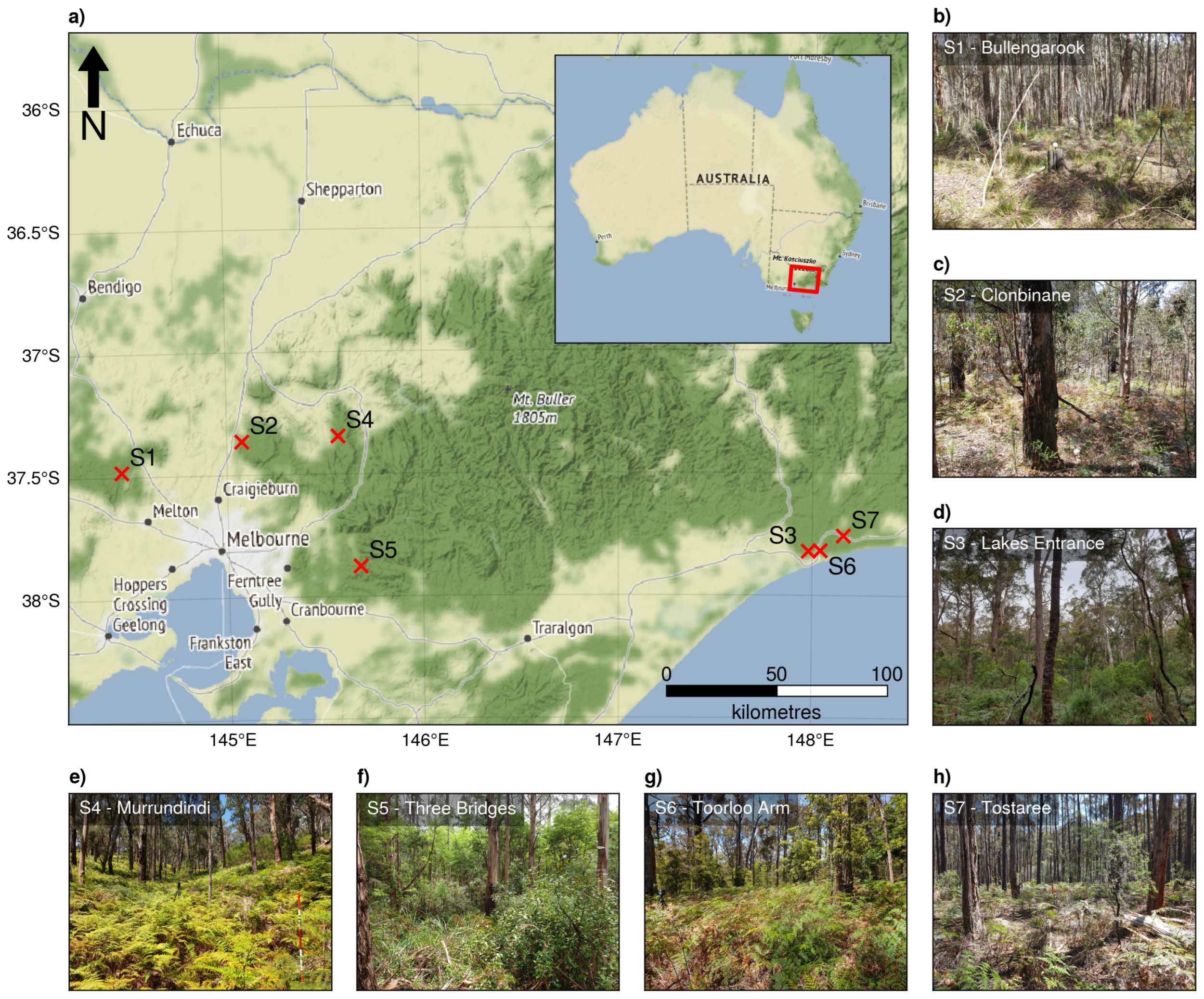
2.1. Study Area

In this study, seven sites (within burn units provided by the local land management agency, where a burn unit is a discrete unit of land that will be treated by prescribed fire) consisting of dry, lowland, and wet Eucalypt forests distributed across Victoria, Australia were included (Figure 1). Sites were selected to be accessible, contain a range of fuel hazard and vegetation conditions, and coincide with the recent (within the last 10 years) capture of ALS data (

Table 1. The properties of the seven study sites used in this study. Date of last burn was provided by the Victorian Department of Environment, Land, Water, and Planning. The type and severity of the burn were not available.

Site	Burn Unit Area (ha)	Vegetation Type	Year of Last Burn	Number of Plots
Bullengarook	182.9	Dry forests	2012	11
Clonbinane	384.5	Dry and lowland forests	2009	12
Lakes Entrance	268	Lowland forests	2011	11
Murrindindi	540	Dry forests, lowland forests with gullies of wet forest	2008	8
Three Bridges	482.7	Wet forests, spurs of dry forest	2000	4
Toorloo Arm	242	Lowland forests—significant bracken	1981	8
Tostaree	341.3	Lowland forests	2001	14

).

2.2. Fuel Data

The fuel data used in this study were collected at each plot using two approaches—one using TLS and another using visual assessments following OFHAG, which is the current operational approach used in Victoria, Australia. These in situ approaches both aimed to characterise fuel within 10 $\mathrm{m}$ radius plots. The number of plots at each site is provided in Table 1, with plot locations selected such that plots were situated at least 100 $\mathrm{m}$ and no more than 500 $\mathrm{m}$ away from the road edge within each site.

2.2.1. Terrestrial Laser Scanning

A Faro Focus M70 laser scanner was used to collect scans across all seven sites. Multiple plots were captured (4–14) with plots distributed based on existing land management approaches. The number of plots collected for each site is mentioned in Table 1. At each plot, five scans were collected in a cross-pattern with a central scan and four scans 10 $\mathrm{m}$ from that scan at 90 deg intervals. All together, 340 TLS scans were collected across seven sites. To characterise fuel in a particular plot, the average of the fuel metric values for each layer collected by the five scans was taken. This reduced the number of sample size to 68 for all seven sites. Each scan was captured at a scan resolution of 1/2 and scan quality of 2×. This resulted in a $3.1$ $\mathrm{m}$$\mathrm{m}$ point spacing at a distance of 10 $\mathrm{m}$. Scans were taken at a height between 1.6 and $1.8$ $\mathrm{m}$ from the ground surface to maximise near-field (<4 $\mathrm{m}$ from the scanner) observation of fuel features.

2.2.2. Visual Assessments

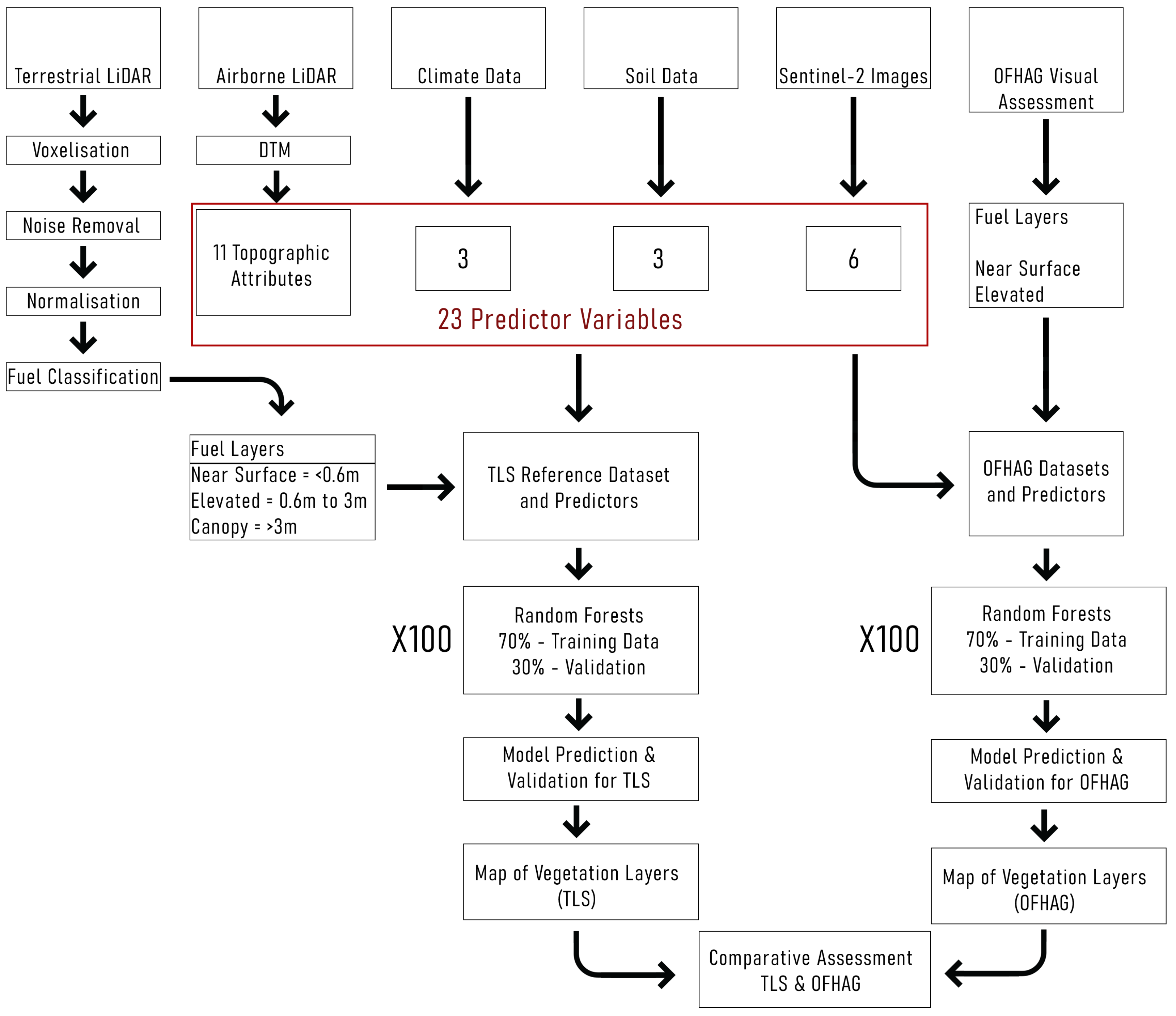
At each plot, a visual assessment following the OFHAG method outlined by Hines et al. [23] was undertaken. Assessments were carried out by personnel from the Department of Environment Land Water and Planning (DELWP) and RMIT University. The number of years of experience for assessors in assessing fuel hazard visually varied from less than one year to 10 years. This process requires an assessment of three different vegetation strata (surface, near-surface, and elevated layers), and an assessment of the bark hazard. Bark hazard is associated with the loose bark on tree trunks and branches, and can create extreme fuel hazards. When assessing each strata, characteristics including the proportion of dead material (near-surface and elevated), the depth (surface), height (where height differentiates fuel layers for separation from a visual standpoint), cover, and arrangement of fuel are visually compared in the field against a set of reference images and descriptions. Estimates of surface and bark fuel attributes made by this method were not considered further in this study, as currently no reliable method exists to observe the characteristics of these layers from TLS data.

3. Method

This study follows the workflow shown in Figure 2. The processing of the TLS data described below produces descriptions of fuel height and cover for the near-surface and elevated layers. In comparison, OFHAG does not explicitly measure near-surface and elevated height [23]. As such, the random forest-based workflow is used to produce landscape-level maps of near-surface and elevated layers cover using both TLS and OFHAG plot observations for training and validation, as well as height using only the TLS observations. Furthermore, the height and cover of the canopy layer is also predicted at landscape level using TLS observations for use in the properties prediction of lower vegetation strata. This section describes the steps taken to pre-process the TLS data and then up-scale response variables for both sets of plot-level data.

3.1. TLS Point Cloud to Fuel Metrics

The workflow outlined in [37,41] was adapted to derive the cover and height of fuel strata from each TLS scan. The main steps of this workflow, including any variations to the parameter used from that of Hillman et al. [37], Wallace et al. [41], are described in this section.

3.1.1. Voxelisation

Each individual scan was first clipped to only include points within a 4 $\mathrm{m}$ horizontal radius from the scanner’s origin to avoid overlap between scans. Then, to provide a discrete representation of the environment, point clouds were transformed into a $0.02$ $\mathrm{m}$ resolution voxel space, where any voxel (or 3D pixel) containing 1 or more points was considered filled. A voxel model for these purposes is a three-dimensional grid domain with the size of the grid cells determining the resolution of the 3D grid [55].

3.1.2. Noise Detection and Removal

Noise was detected within this voxel space using a kNN outlier detection approach [56]. This approach relies on two parameters, the number of nearest neighbours ($nn$) and a standard deviation threshold (ST) where noise points are found by determining the nearest neighbour distance between each point and other points in the point cloud. Points are then considered noise if their nearest neighbour distance is greater than the mean distance plus the standard deviation multiplied by a threshold (ST). Due to the properties of the scanner/environment interaction, it was found that the $nn$ and ST performed better if the (3D) distance to the scanner was considered [41]. The parameters determined in Wallace et al. [41] within a similar environment and using the same scanner were used for this study. These parameters are as follows: for points <2 $\mathrm{m}$ ($nn$ = 18, ST = 1.8), 2–4 $\mathrm{m}$ ($nn$ = 15, ST = 2.6), 4–6 $\mathrm{m}$ ($nn$ = 12, ST = 2.6), >6 $\mathrm{m}$ ($nn$ = 9, ST = 2.6).

3.1.3. Normalisation

Points originating from the ground were detected using the Cloth Simulation Filter (CSF) [57]. In this case, the parameters for the CSF algorithm were set as follows—a cloth resolution of 0.18, a rigidness of 3, a class threshold of 0.03, and a time step of 0.4. These parameters were determined based on the comparison of CSF outcomes on single scans in comparison to manually edited ground points set from a dense multi-scan data collection (reported in [41]). The DTM was constructed by triangular irregular network (TIN) interpolation between the identified ground points. The TIN was then used to normalise the points within each individual scan.

3.1.4. Fuel Strata Classification

Filled voxels were attributed to fuel layers using the layer pouring method outlined in [37]. In brief, the method utilises the vertical layers of the voxel space to determine clusters of filled space. These clusters are determined in the top-most layer first. Where any cluster intersects with a cluster from the layer directly above it, the two clusters are considered to be from the same vegetation element. This then creates a connection of elements through to the ground layer. Once a connection is determined, a cluster is attributed to a fuel strata layer based on the height of the upper-most voxel within the strata. This allows for objects to be allocated to a fuel strata. Although there are no fixed height thresholds defined in the literature for describing fuel strata, we applied an approach consistent with fuel studies in eucalyptus forests. This divides fuel into three classes: the near-surface (<$0.6$ $\mathrm{m}$), elevated ($0.6$ $\mathrm{m}$ to 3 $\mathrm{m}$), and canopy (>3 $\mathrm{m}$) fuel layers [23,37,41,58]. This process was applied on all point clouds to separate those points, which describe the stem and crown elements from the elevated and near-surface and surface elements of the fuel strata.

3.1.5. Fuel Metric Derivation

The cover and height of the near-surface and elevated fuel layers are extracted from the TLS data and used in the landscape level prediction. Canopy height and cover were also determined from the TLS data and predicted at a landscape level.

Mean height was calculated as the mean height of the surface of each fuel layer. The top surface was determined as the highest point within each voxel column. Mean cover was calculated as the number of voxel columns containing at least one voxel from each layer divided by the number of voxel columns containing any filled voxels. In the case of the near-surface layer, the number of columns containing a voxel from this strata was divided by the number of columns containing any voxels from the ground, near-surface, and elevated layers. Once fuel properties were determined for each individual scan, the mean value of the five scans was used to characterise each plot.

3.2. Landscape Fuel Hazard

3.2.1. Random Forest Model Configuration

In order to predict fuel properties across the landscape, random forest regression as implemented in Scikit-learn [59] was used. Random forest was chosen as it has been shown to provide high accuracy and allows for our results to be compared against similar outputs from within the literature [15,27].

For optimal performance of the random forest, two hyper-parameters were tuned—mtry (the number of variables used in each replicate run) and ntree (the total number of independent trees). Predictions were made for the training dataset with ntree values from 200 to 1000. We found that the ntree parameter did not differ significantly with increasing ntree values > 500, the default in many random forest regression modelling studies. Thus, 500 independent trees were used. We considered five possible values for mtry: default (square root of the number of input features), 3, 4, 6, and 9. The default value yielded the lowest out-of-bag error and was used for subsequent modelling.

Separate random forest models were produced for each fuel structural variable derived from the TLS point clouds and the visual assessments. As the understorey vegetation conditions are likely dependent on the canopy properties, a sequential approach was used to predict fuel properties using the TLS data [60]. In this approach, the canopy properties (height and cover) were predicted with the output used as parameters in the prediction of near-surface and elevated fuel properties. This approach was not followed using the OFHAG assessments as no canopy observations were recorded.

The four key drivers of vegetation distribution: topography [61], climate, soil [62], and vegetation indices from Sentinel-2 [63] (detailed below and described in Appendix A) were used as predictor variables. These predictor variables were chosen based upon a review of the literature and were considered to have an explanatory relationship with vegetation structure and composition in the study sites [15,27,61,63,64,65,66]. The final model was produced with a 20 $\mathrm{m}$ resolution to be commensurate with the plot area (10 $\mathrm{m}$ radius) and the resolution of landscape predictor variables.

3.2.2. Topographic Variables from ALS

ALS point clouds were used to produce a digital terrain model (DTM) at a spatial resolution of 20 $\mathrm{m}$ using pre-classified ground points and blast2dem tool within lastools [61]. These point clouds were obtained from the Victorian State Government (DELWP). At each site, data were collected using a range of ALS sensors, with capture properties also differing including the target pulse densities (

Table 2. Properties of the Airborne Laser Scanning data collected at seven sites.

Site Name	Date of Capture	ALS Sensor	Pulse Density (pts/m${}^2$)
Bullengarook	2017–2018	Trimble AX-60	8
Clonbinane	2019	Trimble AX-60	9.45
Lakes Entrance	2019	Riegl VQ780	8
Murrindindi	2016	Trimble AX-60	4
Three Bridges	2016	Trimble AX-60	4
Toorloo Arm	2019	Riegl VQ780	8
Tostaree	2019	Riegl VQ780	8

). QGIS software was then used to derive eleven topographic attributes (

Table A1. Topographic attributes derived from DTM using ALS data at a spatial resolution of 20 $\mathrm{m}$ for each site.

Topographic Variables	Description
Slope	Calculated by fitting a plane to the eight neighbouring cells [87].
Aspect	The orientation of the cell relative to the north [87].
Catchment area	The upstream area of each cell [88].
Profile curvature	The rate of change of slope in a down-slope direction: a proxy for acceleration and deceleration of water over the terrain [89].
Plan curvature	The curvature of a contour at the central pixel. It can be used as a proxy for convergence and divergence of water [89].
Potential solar radiation ratio	The ratio of the potential solar radiation on a sloping surface to that on a horizontal surface [90].
Topographic Position Index	Classifying terrain such that the altitude of each data point is evaluated against its neighbourhood to verify whether any particular data point forms part of a positive (e.g., crest) or negative (e.g., trough) feature of the surrounding terrain [91].
Terrain Ruggedness Index	The sum change in elevation between a grid cell and its eight neighbouring grid cells [92].
Stream Power Index	A measure of the erosive power of flowing water [93].
Topographic Wetness Index	A measure of soil moisture potential that combines contextual and site information and is used to identify potential locations of ephemeral gullies [94].
Convergence Index	The average bias of the slope directions of the adjacent cell from the direction of the central cell minus 90 degrees [88].

) from the DTM at a spatial resolution of 20 $\mathrm{m}$.

3.2.3. Soil Variables from Soil Data

Following the findings from McColl-Gausden et al. [27], three soil variables (bulk density, clay content, pH CaCl${}_2$) were used as predictor variables. These were obtained from CSIRO Data Access Portal at a resolution of 3 × 3 arcseconds ≈90 × 90 $\mathrm{m}$, (www.clw.csiro.au/aclep/soilandlandscapegrid/index.html (accessed on 16 March 2022)) [67]. The raw soil data were provided for three depths (0–5, 5–15, 15–30 $\mathrm{c}$$\mathrm{m}$). However, only the top-most layer for each soil variable was included due to high correlations among the depths [62]. Soil variables were then resampled at a spatial resolution of 20 $\mathrm{m}$ using cubic convolution approximation resampling approach.

3.2.4. Climate Variables from Climate Data

Climate data were downloaded from Worldclim at a resolution of 1 $\mathrm{k}$$\mathrm{m}$${}^2$ (http://worldclim.org/version2) (accessed on 16 March 2022) [68]. These were summarised into annual mean temperature, maximum temperature of warmest month, and precipitation of warmest quarter following McColl-Gausden et al. [27] and resampled using a cubic convolution approximation resampling approach to a spatial resolution of 20 $\mathrm{m}$.

3.2.5. Vegetative Indices from Sentinel MSI-2

Sentinel 2A multi-spectral imagery captured within 60 days of the plot data acquisition was downloaded from Google Earth Engine. Cloud-free composites of Level-2A imagery from acquisitions between November 2021 and January 2022 were created. From this imagery, seven individual bands (B1–B7) were obtained. Following [63,65], we then calculated the chlorophyll red-edge index, shortwave infrared to near infrared ratio, tasseled cap greenness, and tasseled cap wetness specific to the Sentinel-2 data [63] at a spatial resolution of 20 $\mathrm{m}$.

3.3. Model Evaluation

For each fuel property, values were extracted from the raster dataset at the location of each plot using the nearest neighbour approach. In each case, these sample points were divided into a training dataset (70%) and a validation dataset (30%). This was repeated 100 times to remove any bias from the selection of these groups [69,70,71]. For final performance, average results were presented.

The resultant models were used to predict each fuel metric derived from TLS data at a landscape level. As cover estimates for visual assessments were available only for near-surface and elevated layers, the following comparisons between visual and TLS estimates were only based on these layers.

The random forest regression models for each fuel metrics were parameterised using the out-of-bag (OOB) score ($R^2$). OOB accuracy assessments provided by random forest are claimed to be reliable [72]. Random forest based on the out-of-bag concept does not need a separate testing set to evaluate the model [73], while the success of the model against the held-out validation data was assessed via root mean square error (RMSE) and Pearson correlation coefficient (r) [74,75]. The mean value and standard deviation were recorded for each set of training and validation data. For final performance statistics, average results were presented.

4. Results

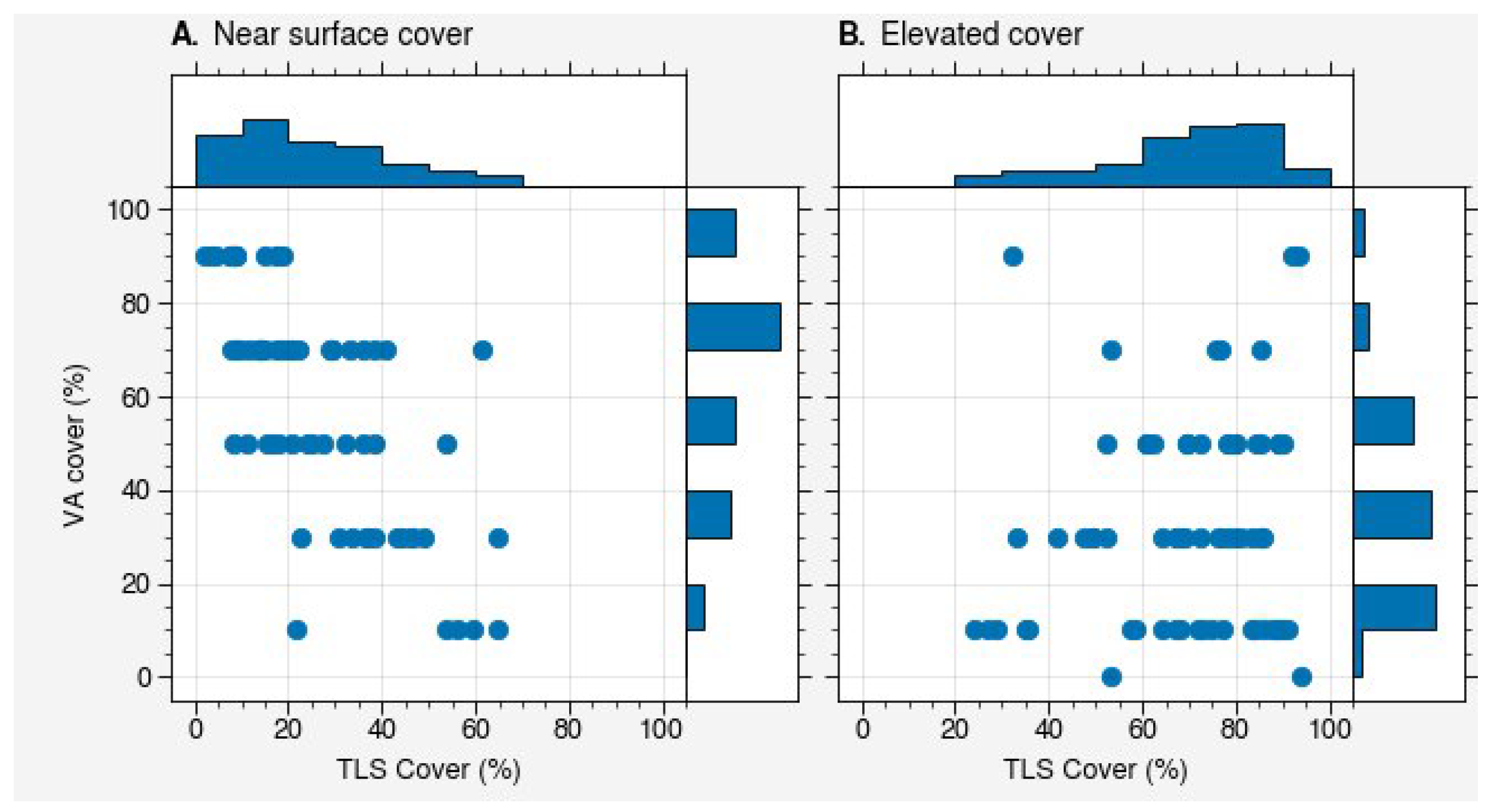
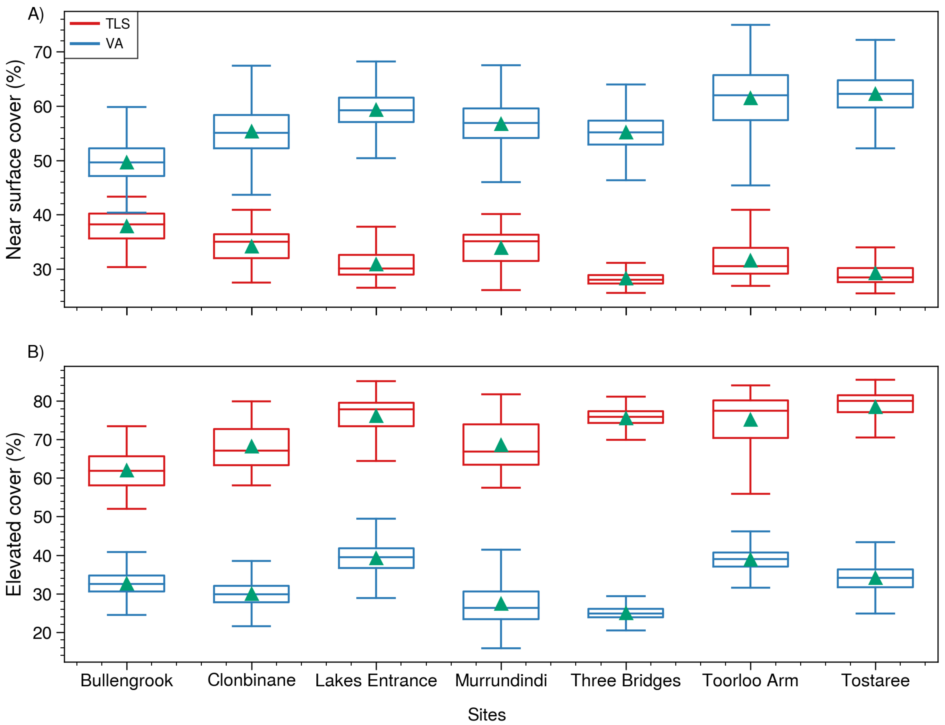
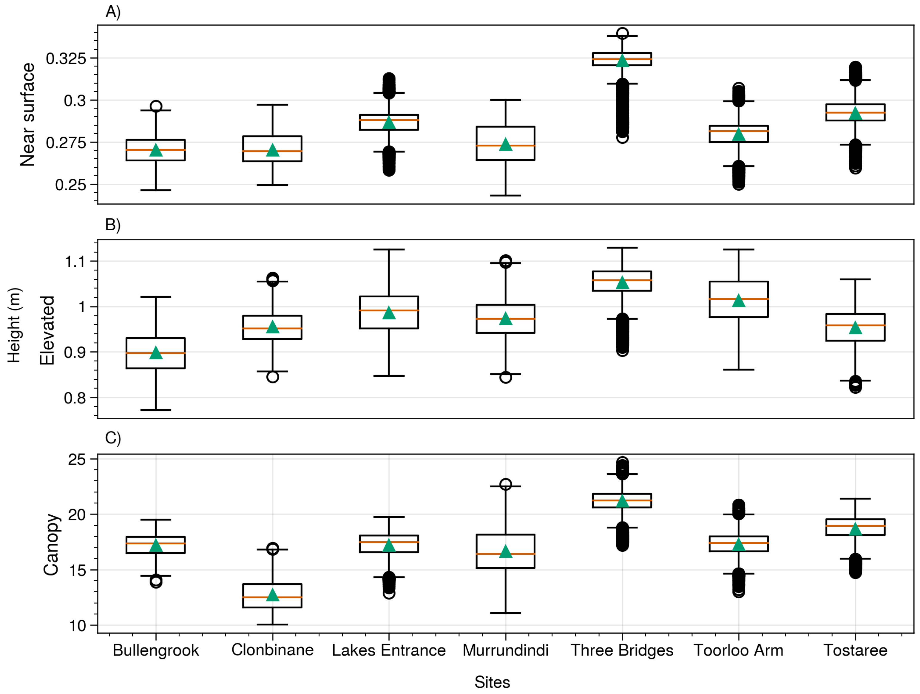
4.1. Plot-Level Fuel Estimates

Elevated fuel cover estimates from TLS and the visual assessment approaches showed low correlation (r = 0.14) (Figure 3B). The cover estimates observed using TLS point cloud ranged from 24.2 to 93.7% (mean = 69.6, median = 73.8). However, visually assessed cover estimates ranged from 0 to 90% (mean = 32.4, median = 30). For the near-surface layer, a negative correlation (r = −0.71) was observed between two estimates (Figure 3A). In most cases, the TLS estimates of cover (mean = 26%) were lower than the visual estimates (mean = 59%) (Figure 3A). The cover estimates observed using TLS point cloud ranged from 2 to 65%, whereas visually assessed cover estimates ranged from 10 to 90%.

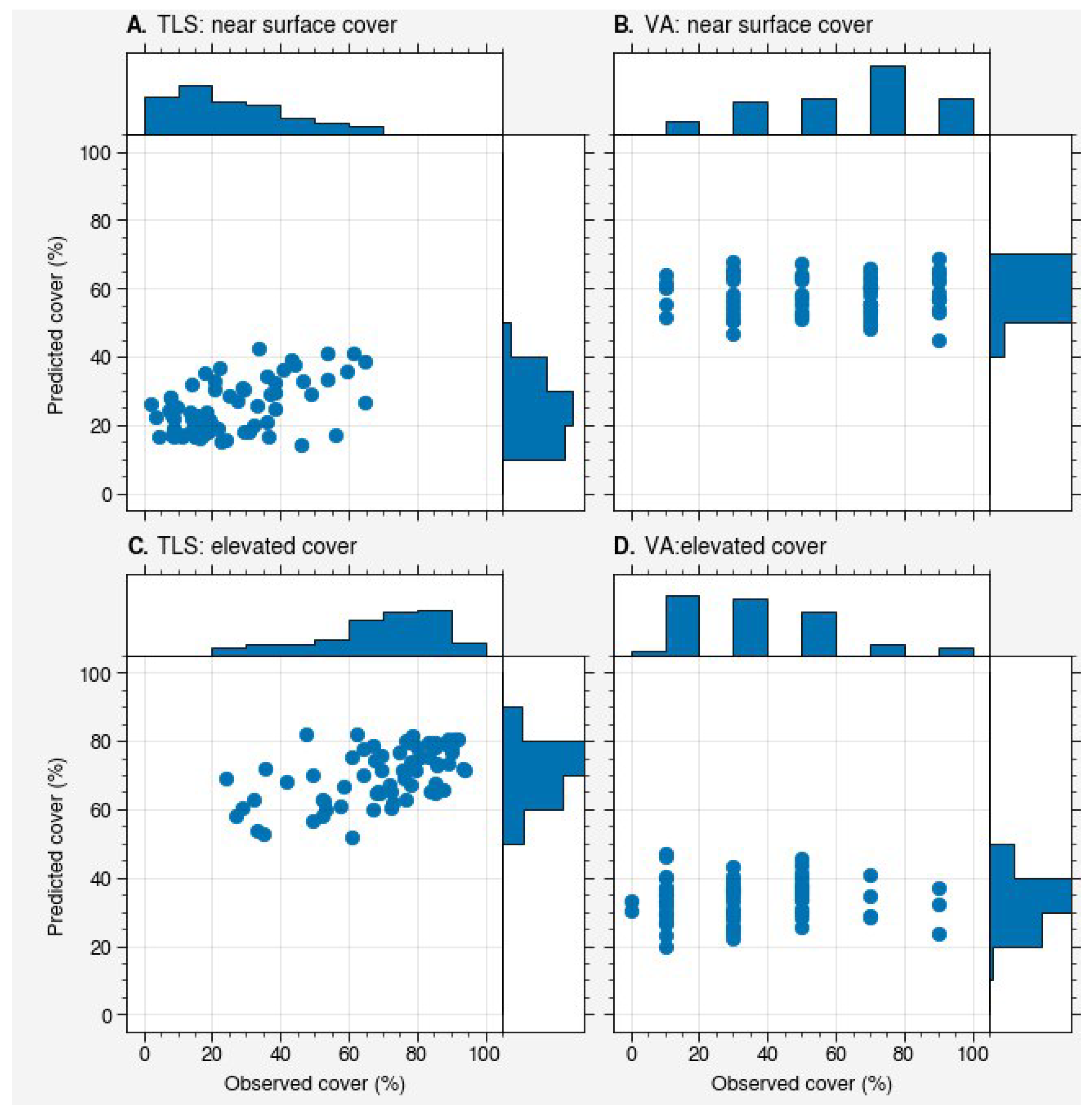
4.2. Random Forest Model Predictions for Near-Surface and Elevated Fuel Cover

The Random forest model trained and validated with the TLS estimates was found to have higher predictive power than the model trained with visually assessed estimates (Figure 4). The OOB score was found to be positive for both layers when predicted using TLS estimates and negative ($R^2$ = −0.1) for estimates predicted using visual assessments (

Table 3. Summary results showing mean ($\mu$) and standard deviation ($\sigma$) of out-of-bag score (OOB), Pearson coefficient of correlation (r), and RMSE for cover and height estimates from the TLS and visual assessment approaches (VAs). Statistics for visual assessments are available only for near-surface and elevated cover.

Fuel Metrics	Approach	${\mathit{R}}^2$ (OOB)		r		RMSE
		$\mathbf{\mu }$	$\mathbf{\sigma }$	$\mathbf{\mu }$	$\mathbf{\sigma }$	$\mathbf{\mu }$	$\mathbf{\sigma }$
Near-surface cover (%)	TLS	0.51	0.07	0.5	0.16	15	2.1
	VA	−0.1	0.09	0.04	0.18	25	2.6
Elevated cover (%)	TLS	0.31	0.09	0.55	0.14	16	2.4
	VA	−0.1	0.09	0.12	0.17	23	3.3
Canopy cover (%)	TLS	0.10	0.08	0.38	0.15	12	1.70
Near-surface height (m)	TLS	0.23	0.08	0.47	0.11	0.04	0.01
Elevated height (m)	TLS	−0.09	0.11	0.12	0.22	0.22	0.04
Canopy height (m)	TLS	0.25	0.07	0.6	0.15	4.41	0.62

). As such, the predictions of cover for both layers from the random forest models trained with TLS estimates were found to have higher correlation as well as lower RMSE in comparison to models based on visual estimates (Table 3).

The models for each variable predicted a restricted range of cover estimates in comparison to the field observations (Figure 4). In case of the TLS model, cover predictions ranged from 14.24% to 42.58% for near-surface (Figure 4A) and 52.01% to 81.84% for elevated layers (Figure 4C). However, field observation of cover using TLS ranged from 1.98% to 64.8% for near-surface and 24.21% to 93.74% for elevated layers.

A similarly restricted range of cover was predicted from the model trained with visual assessments in comparison to the in-field visually assessed observations. Cover predictions from the model trained with visual assessments ranged from 44.93% to 68.61% in comparison to in-field visual assessment (10% to 90%) (Figure 4B) for near-surface layers and 19.88% to 47.13% in comparison to the in-field visual assessment (0% to 90%) for elevated layers (Figure 4D).

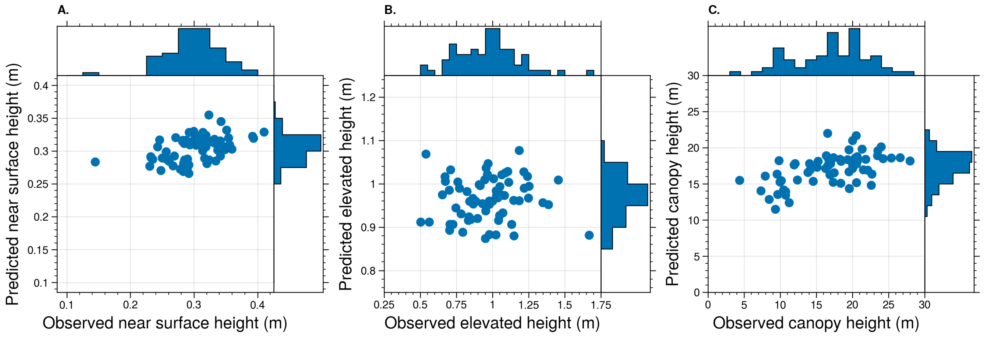
4.3. Fuel Metrics Predicted Using TLS Measurements Only

Canopy cover predicted by the random forest models trained with TLS observations achieved low OOB (R${}^2$ = 0.10), an RMSE of 12%, and a correlation of 0.38 (Table 3). Canopy height predictions on the other hand had higher predictive power (R${}^2$ = 0.25) and exhibited a moderate correlation (r = 0.6) with the validation data; however, low predictions in taller forests resulted in a relatively high RMSE ($4.41$ $\mathrm{m}$) (Figure 5C).

Both elevated and near-surface height models provided low-to-moderate predictive power. The mean predictions of elevated height from the random forest models trained with TLS observations were found to have low correlation (r = 0.12) with elevated height observed using TLS (Figure 5B). The mean predictions of near-surface height from the random forest models trained with TLS observations was found to have moderate correlation (r = 0.47) with near-surface height observed using TLS (Figure 5A).

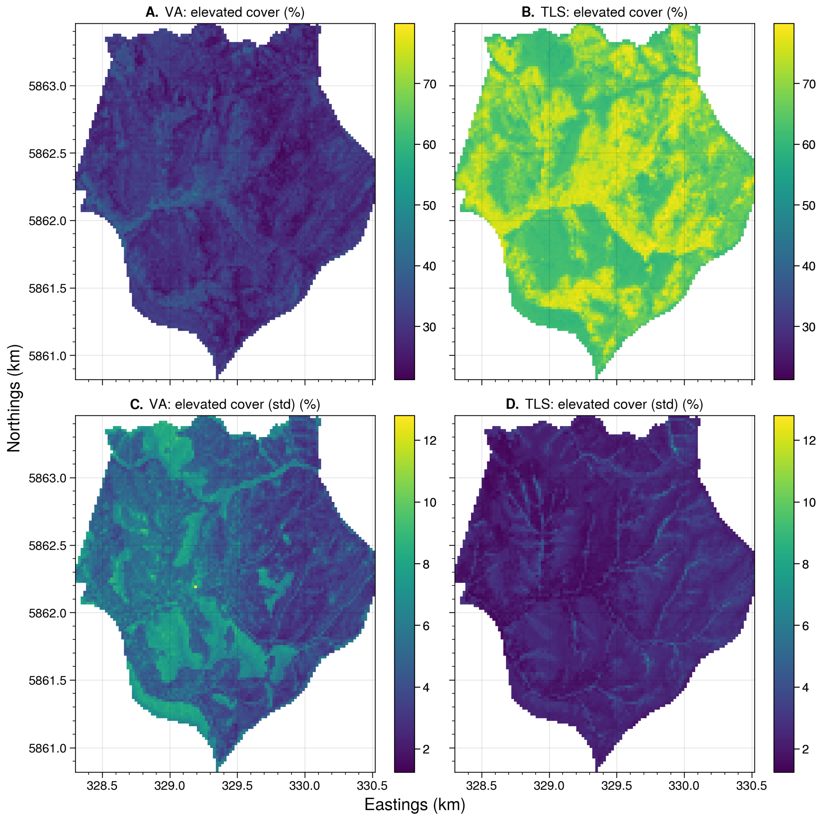
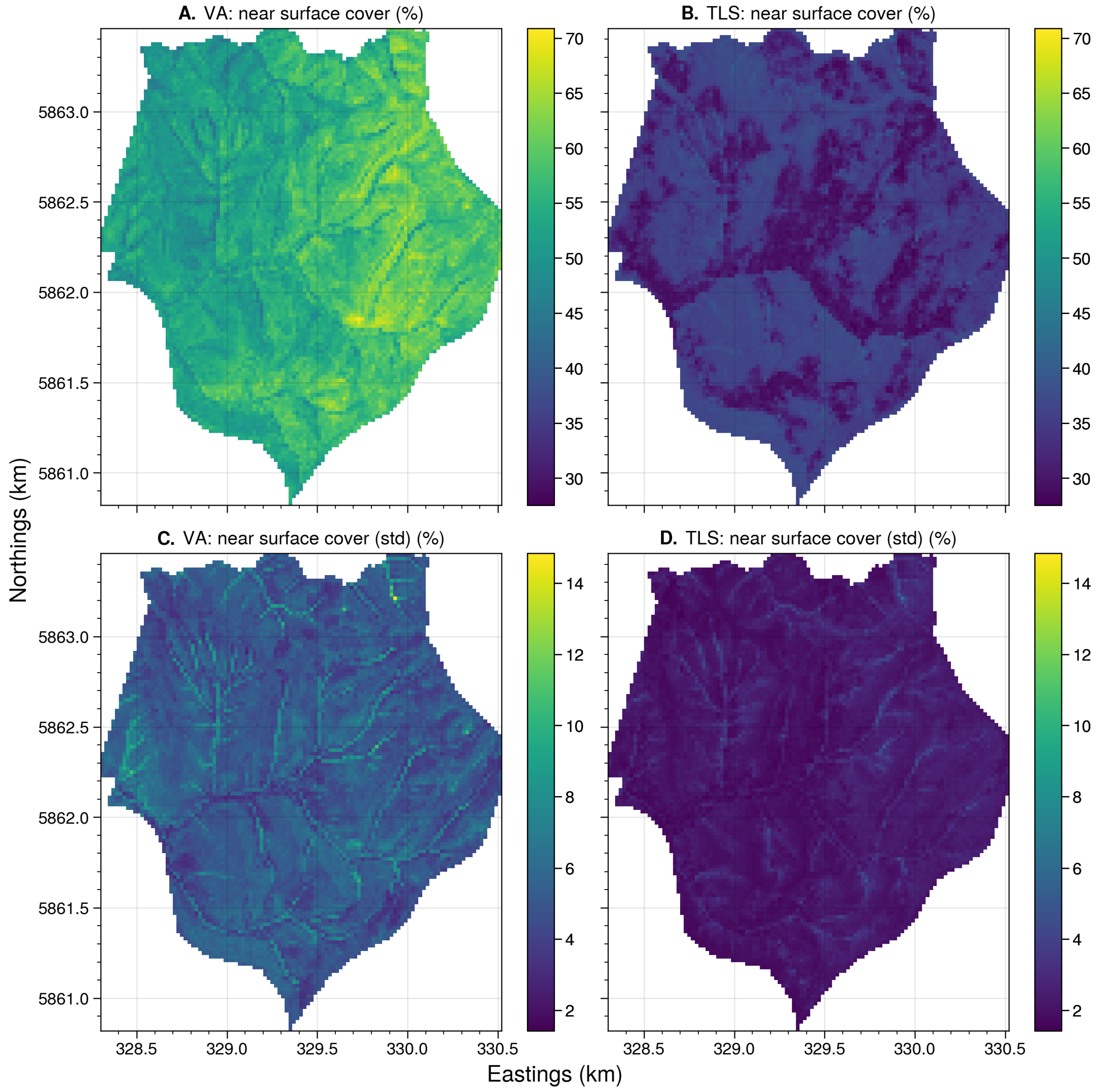
4.4. Landscape Level Fuel Properties

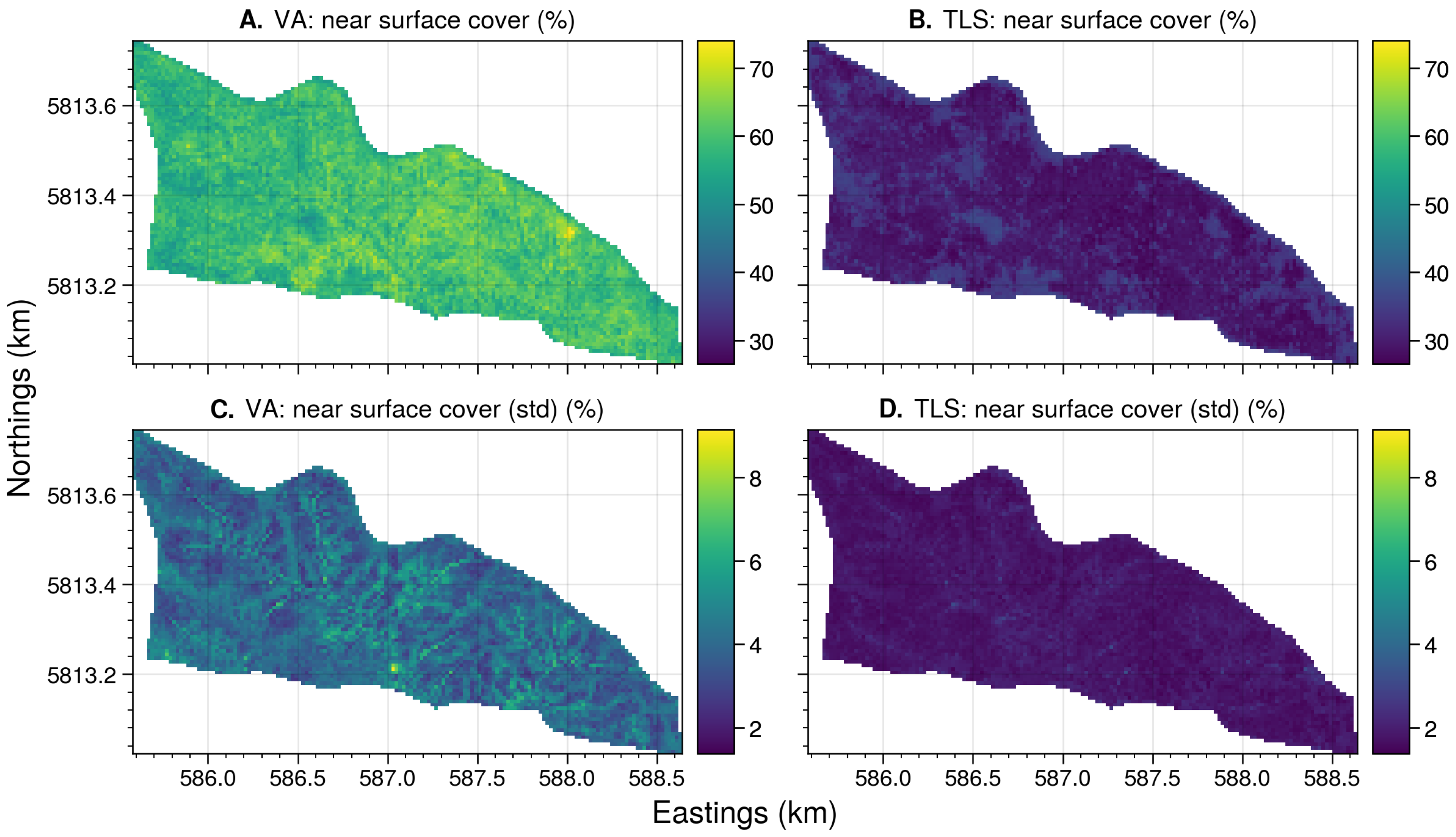
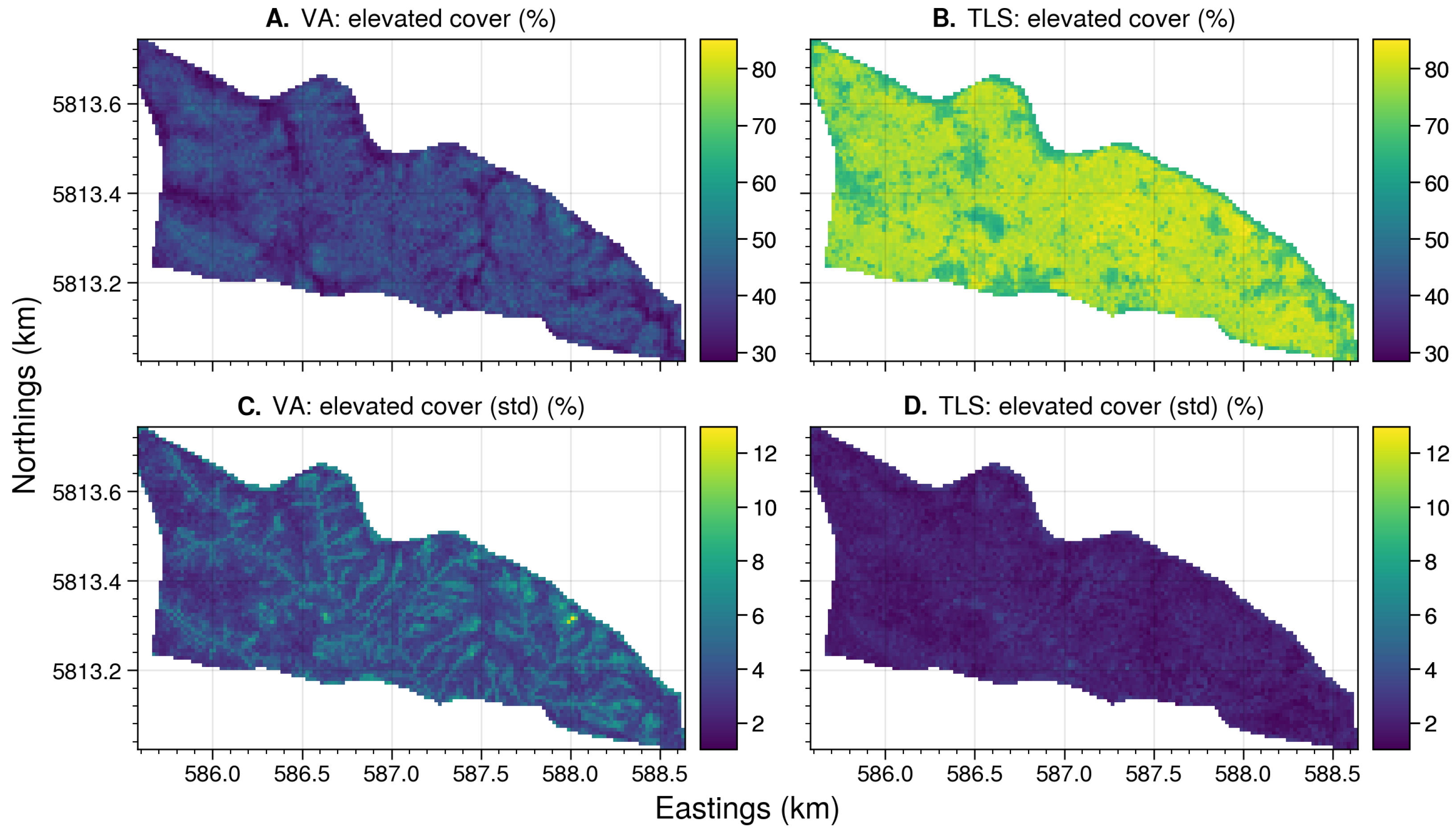
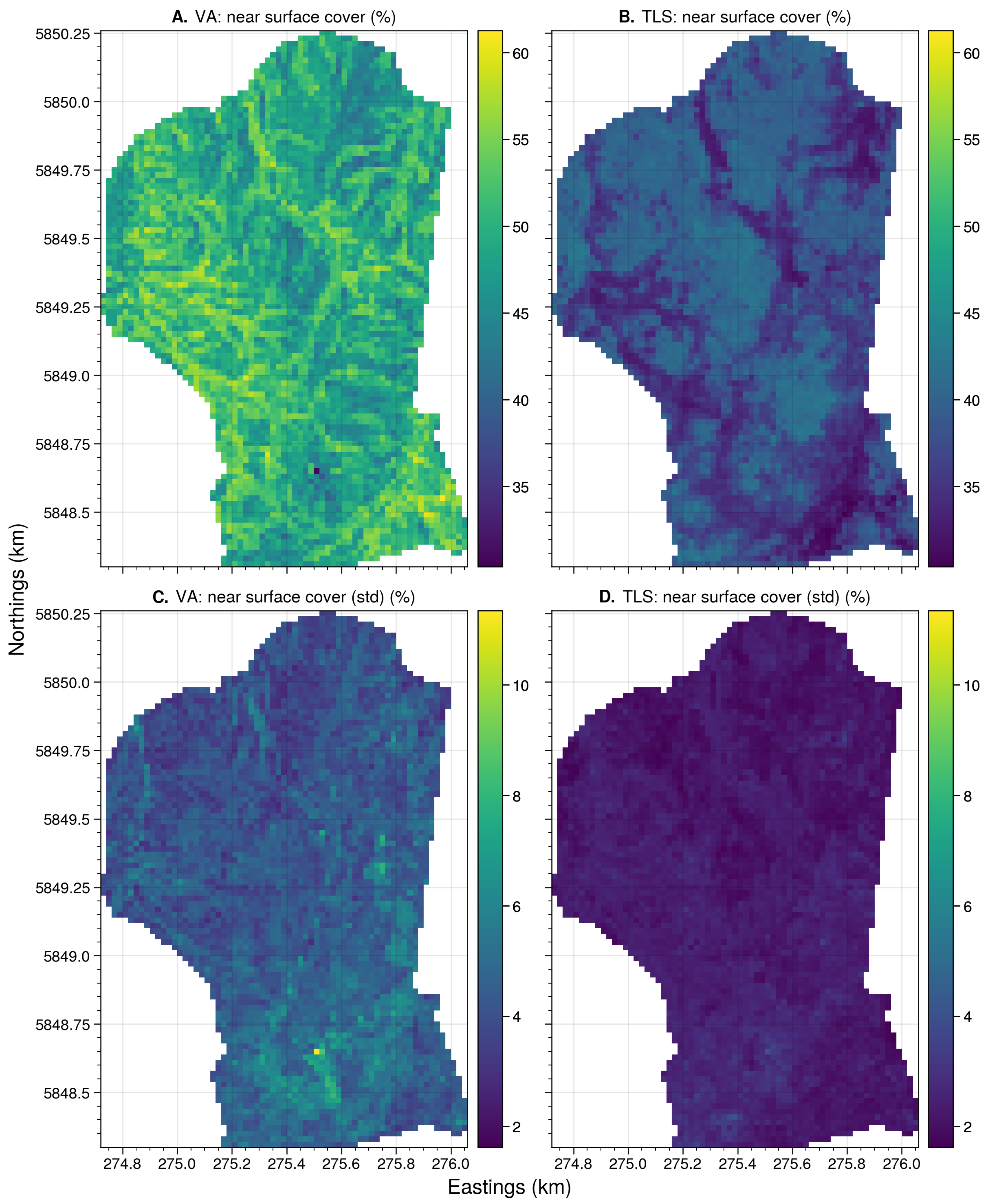
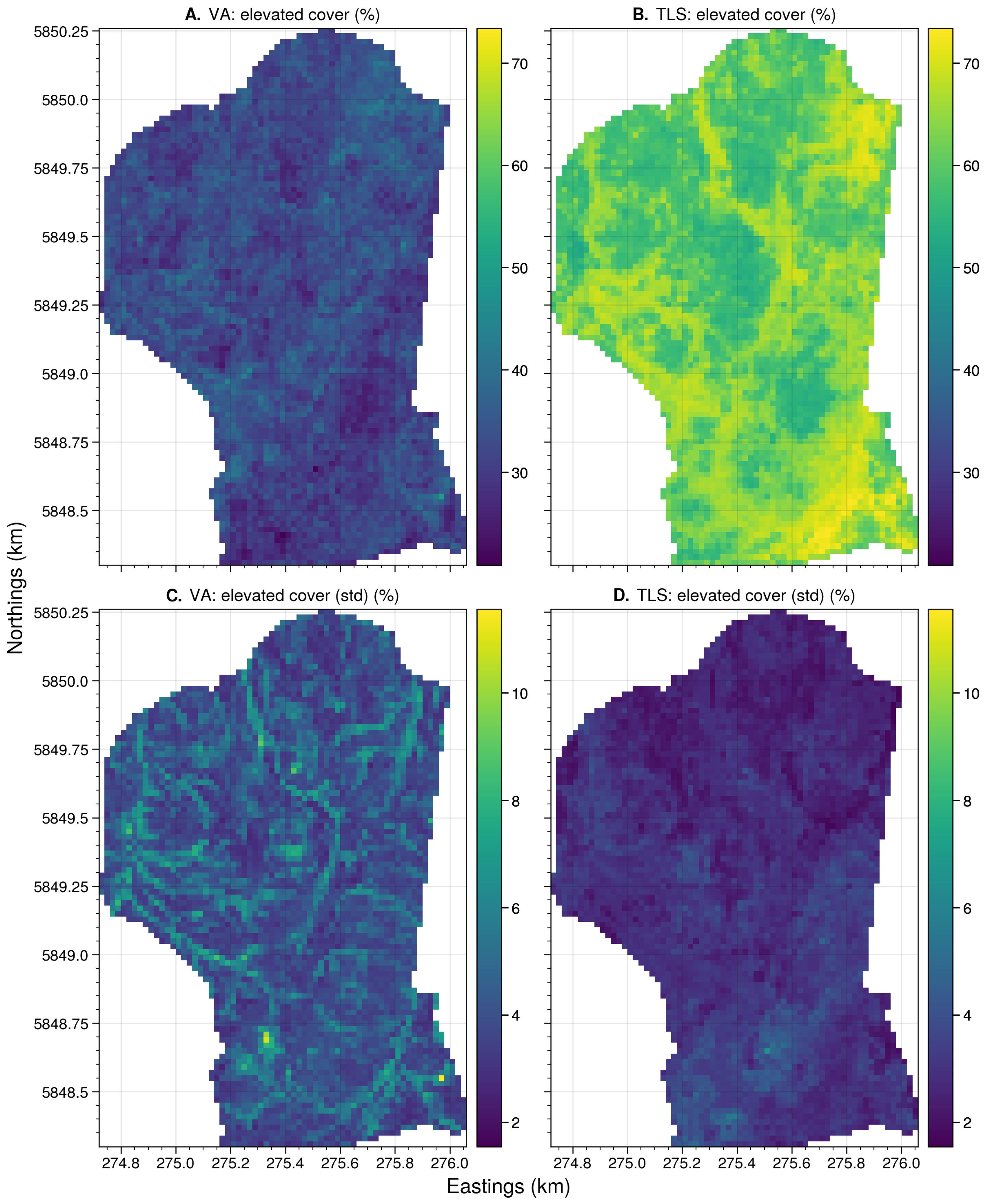
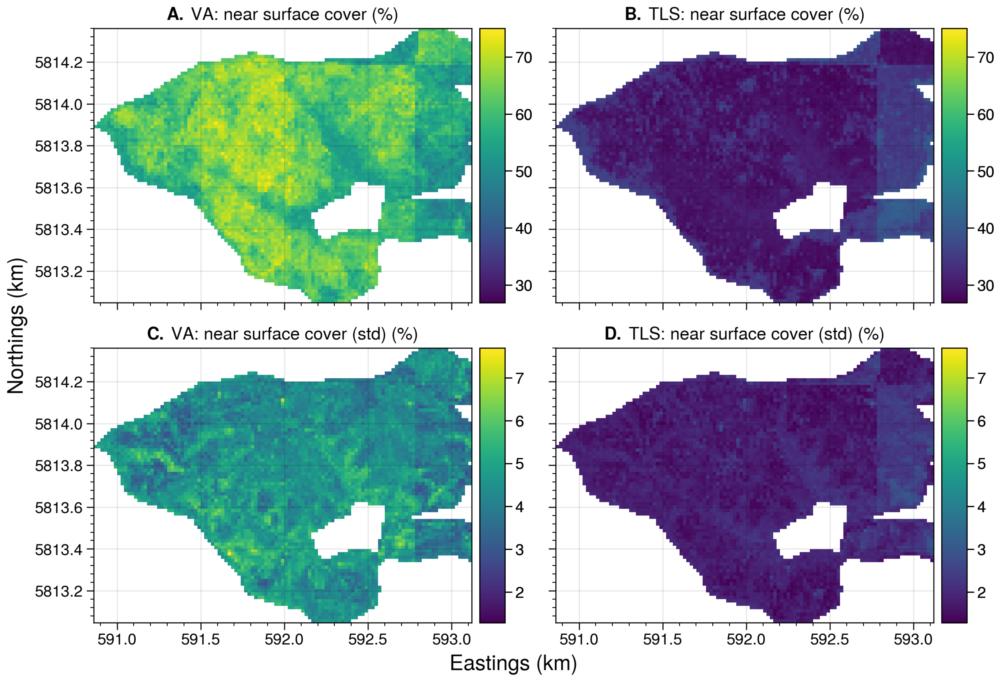
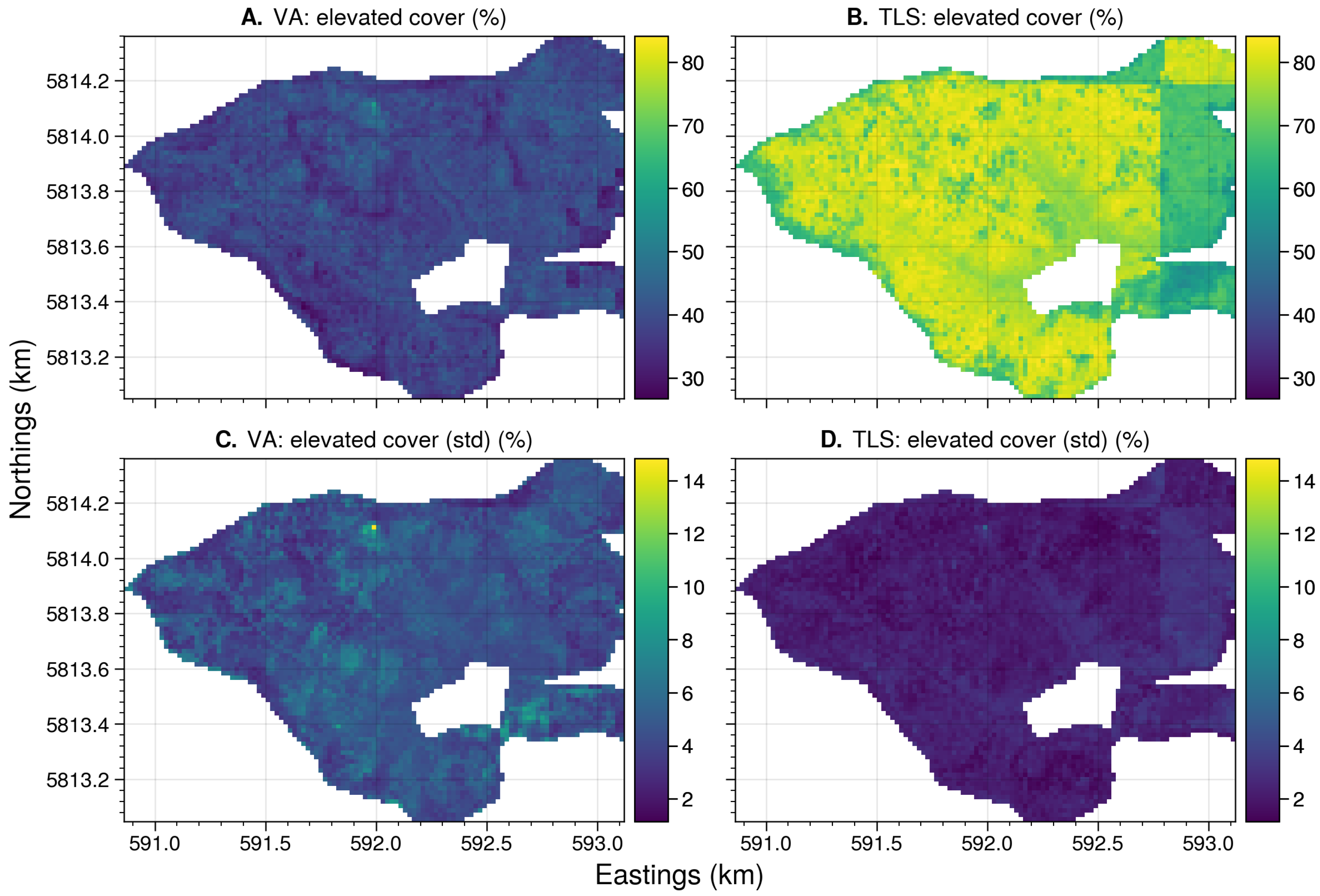
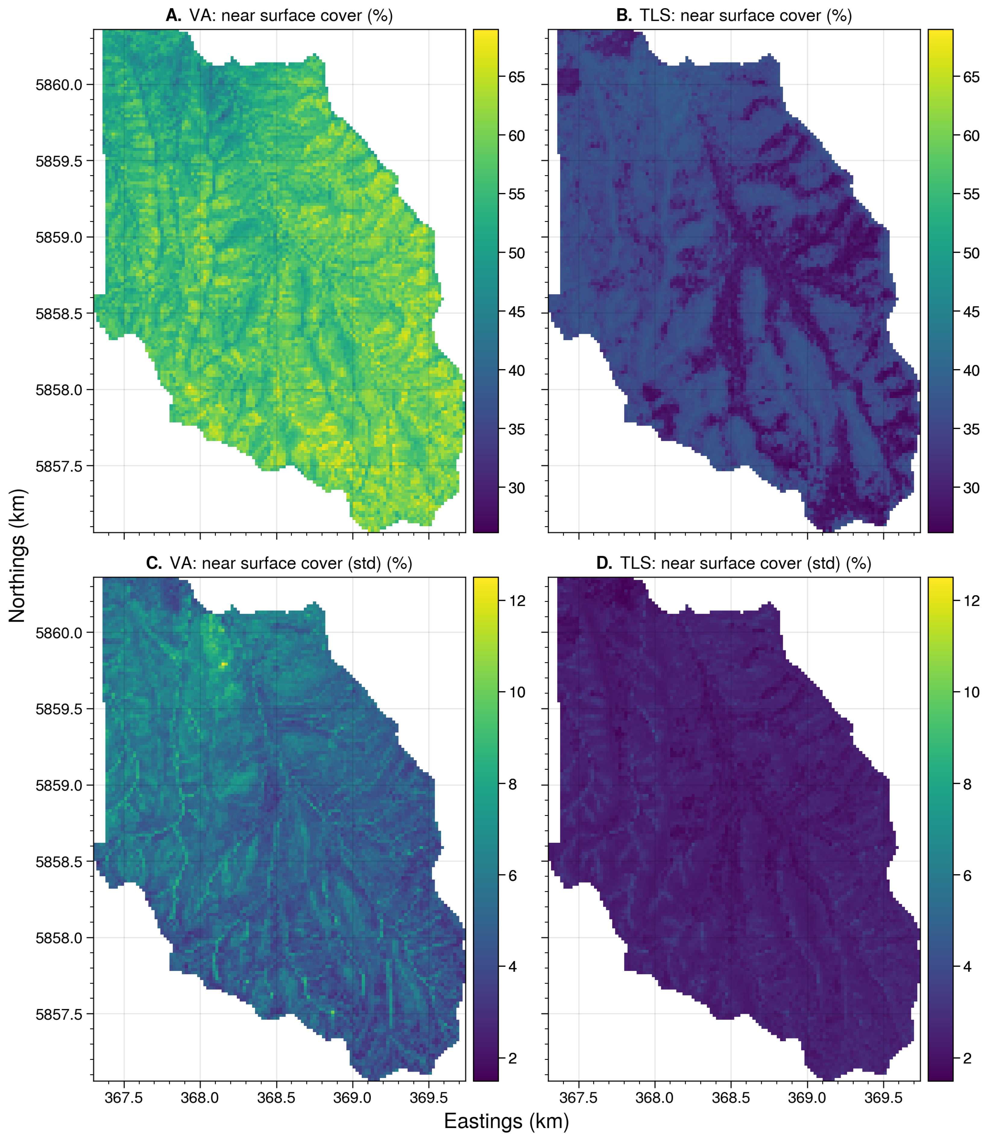
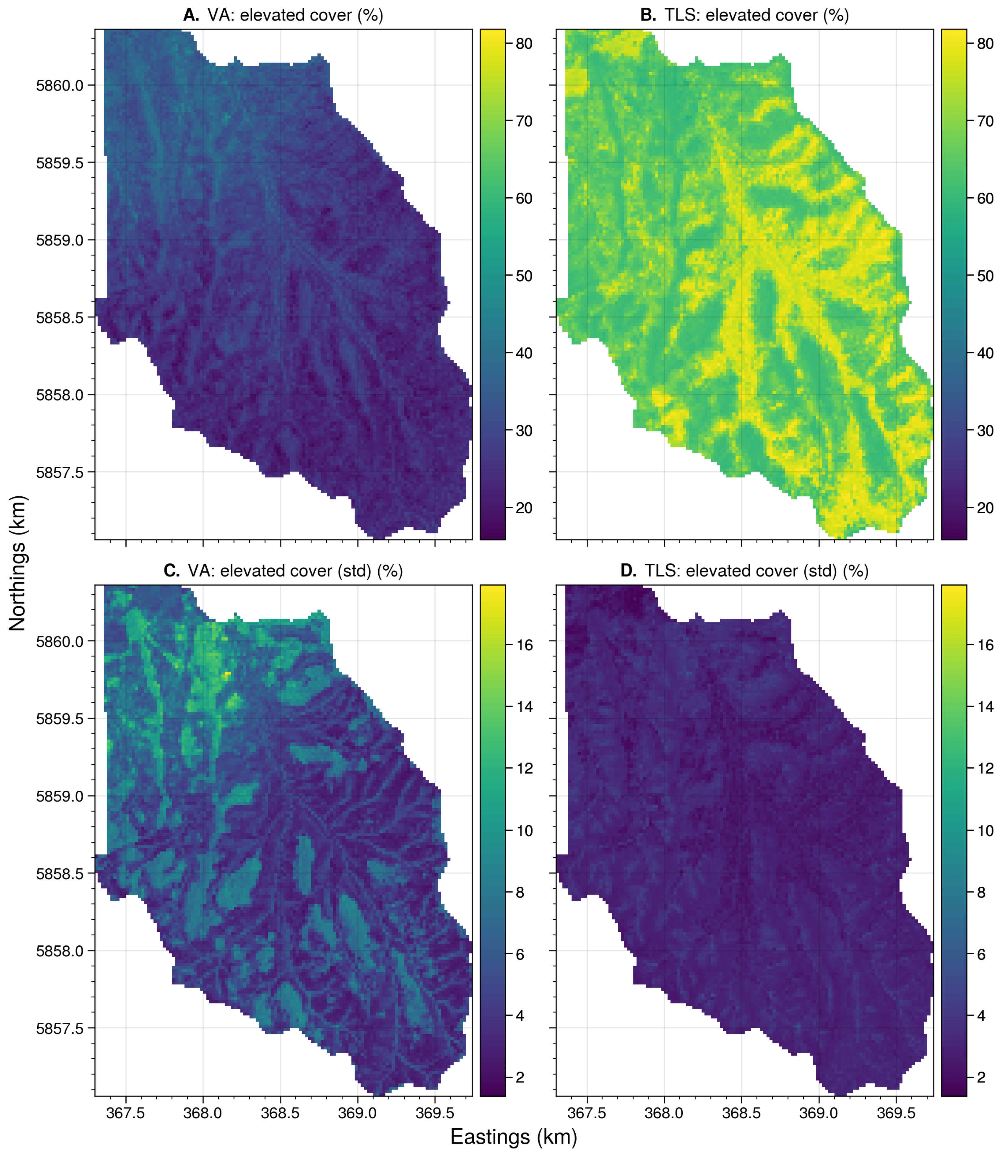
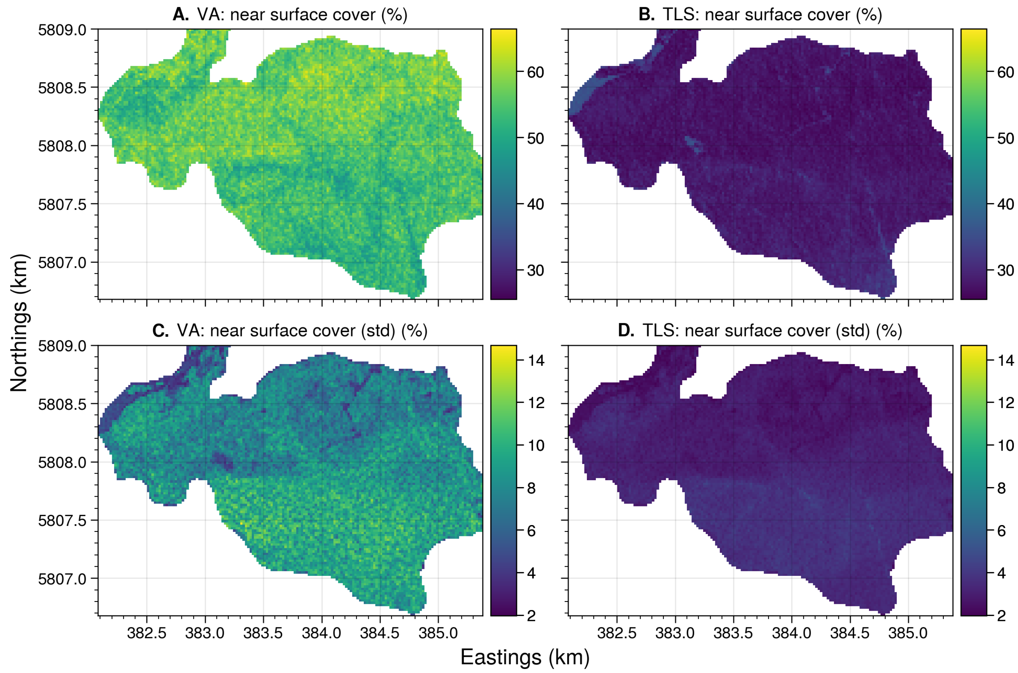
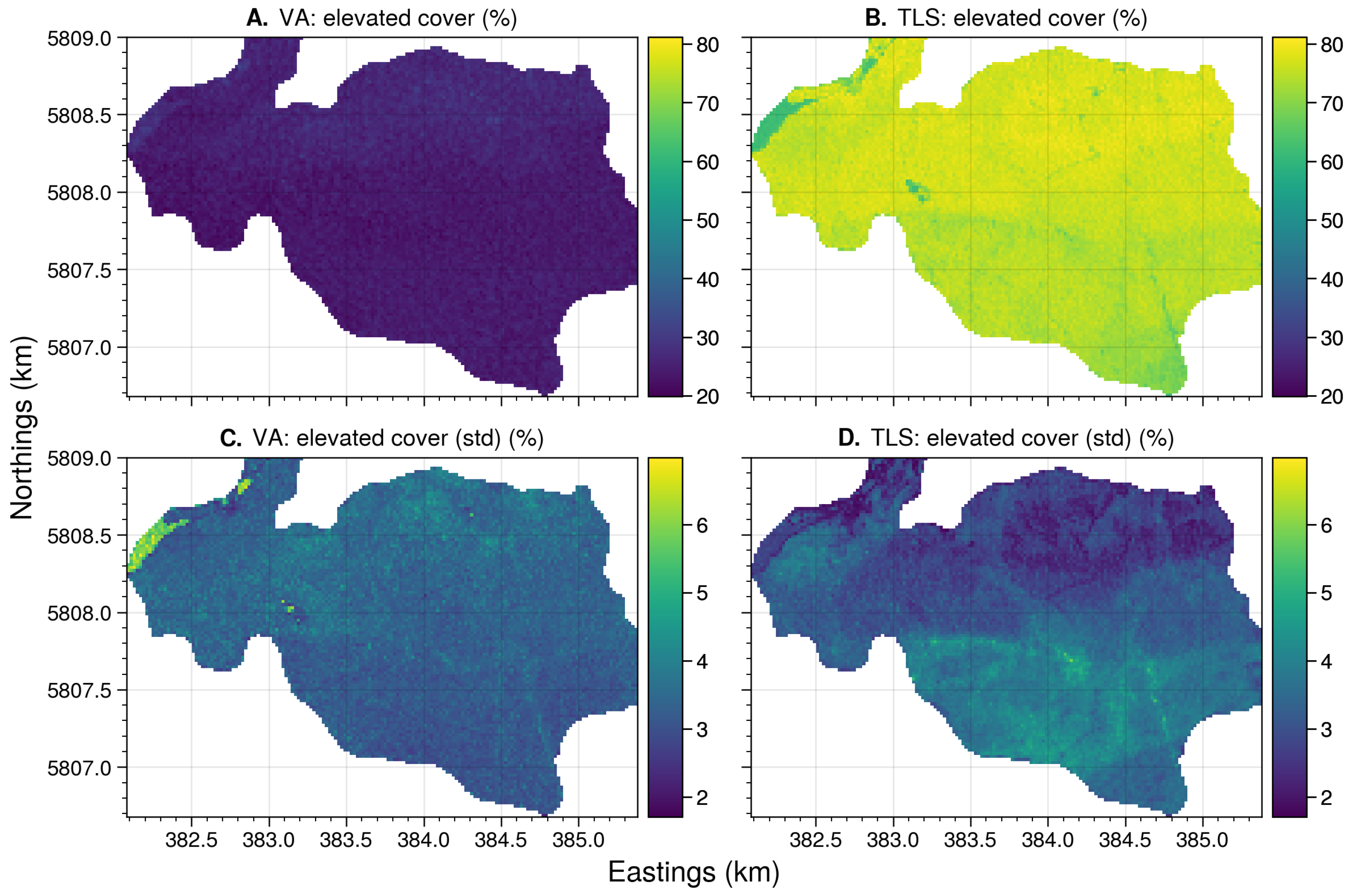
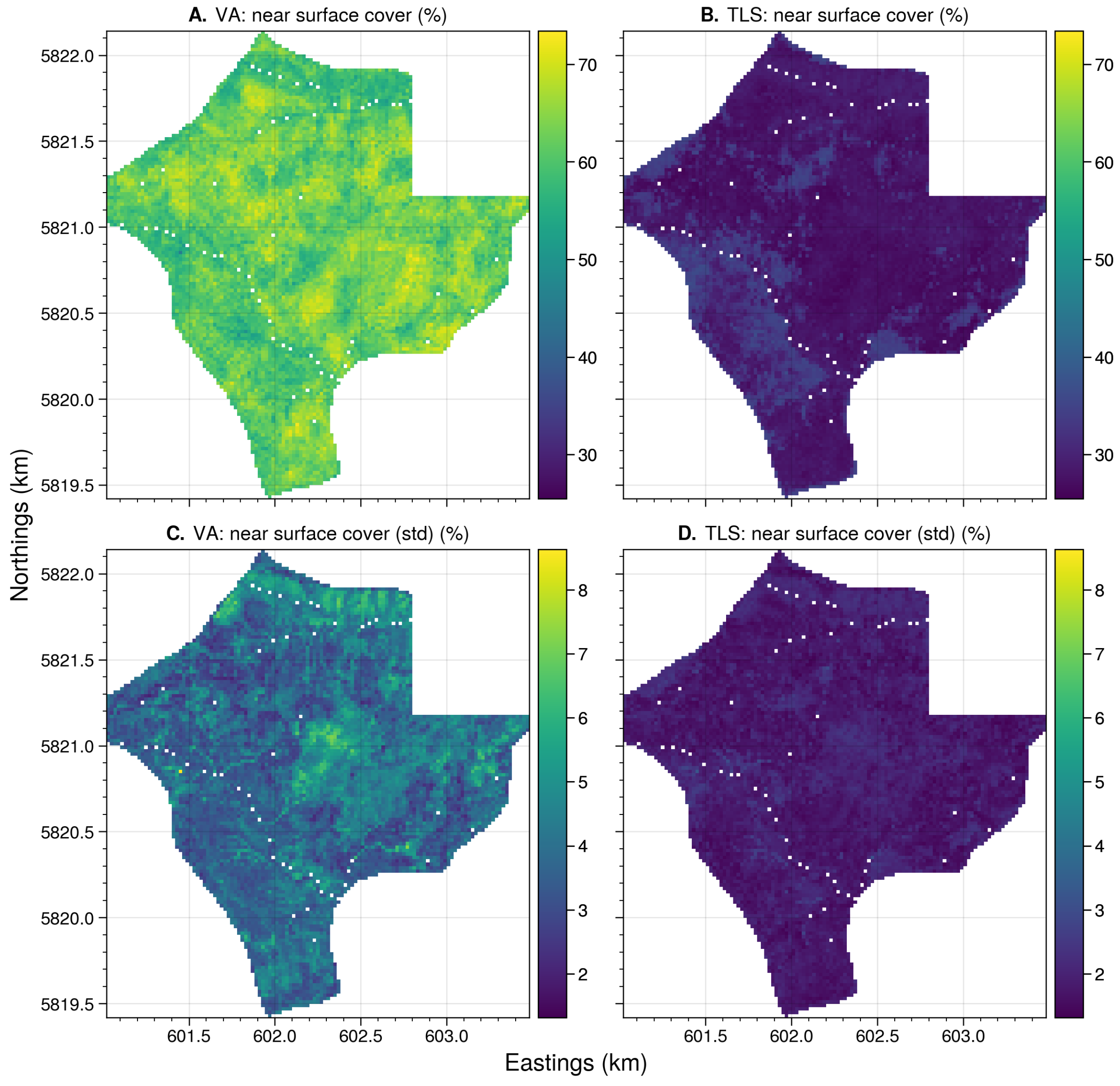
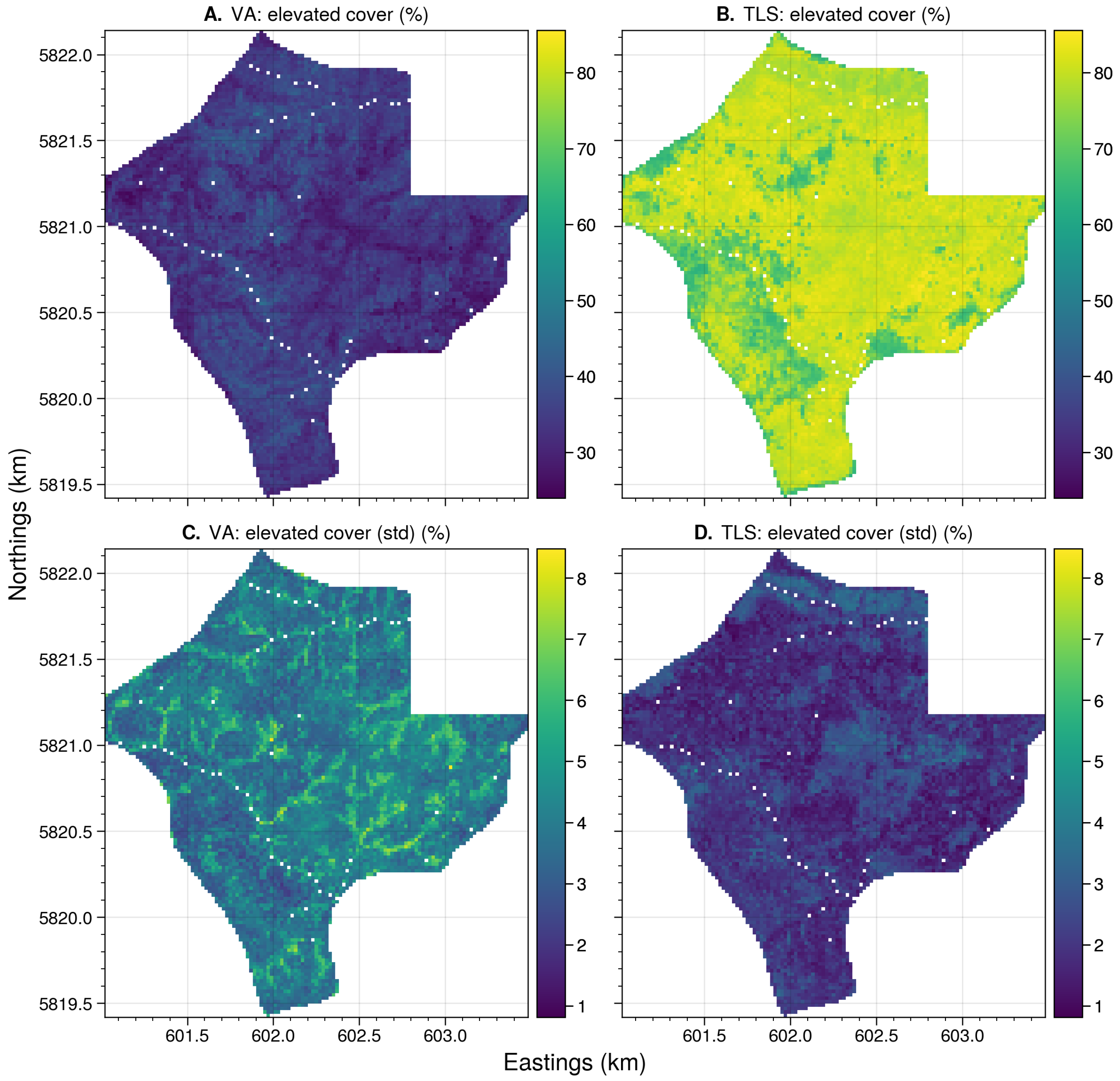
4.4.1. Near-Surface and Elevated Cover

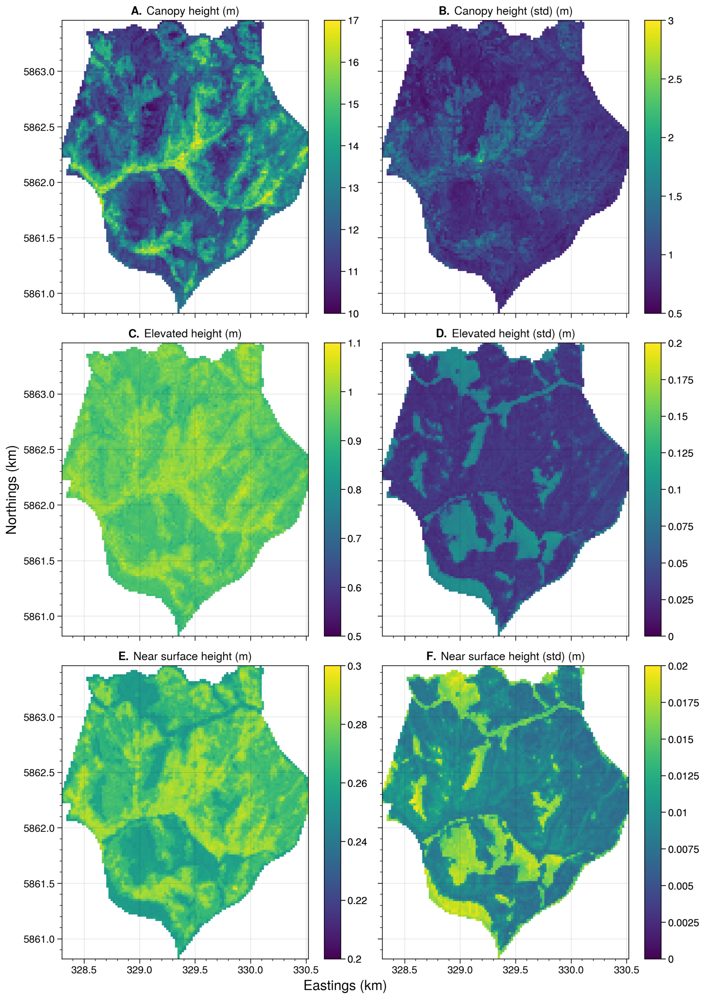
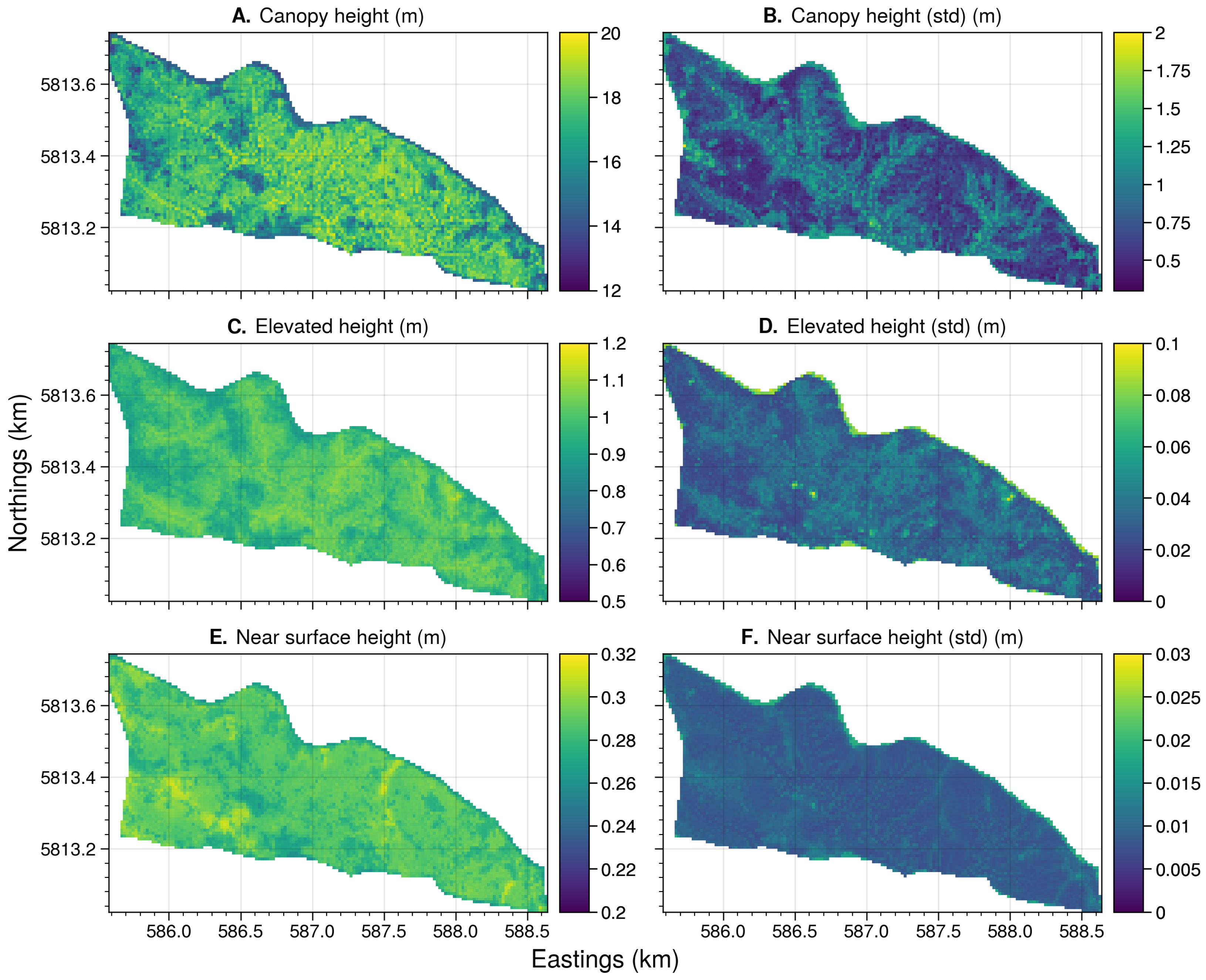
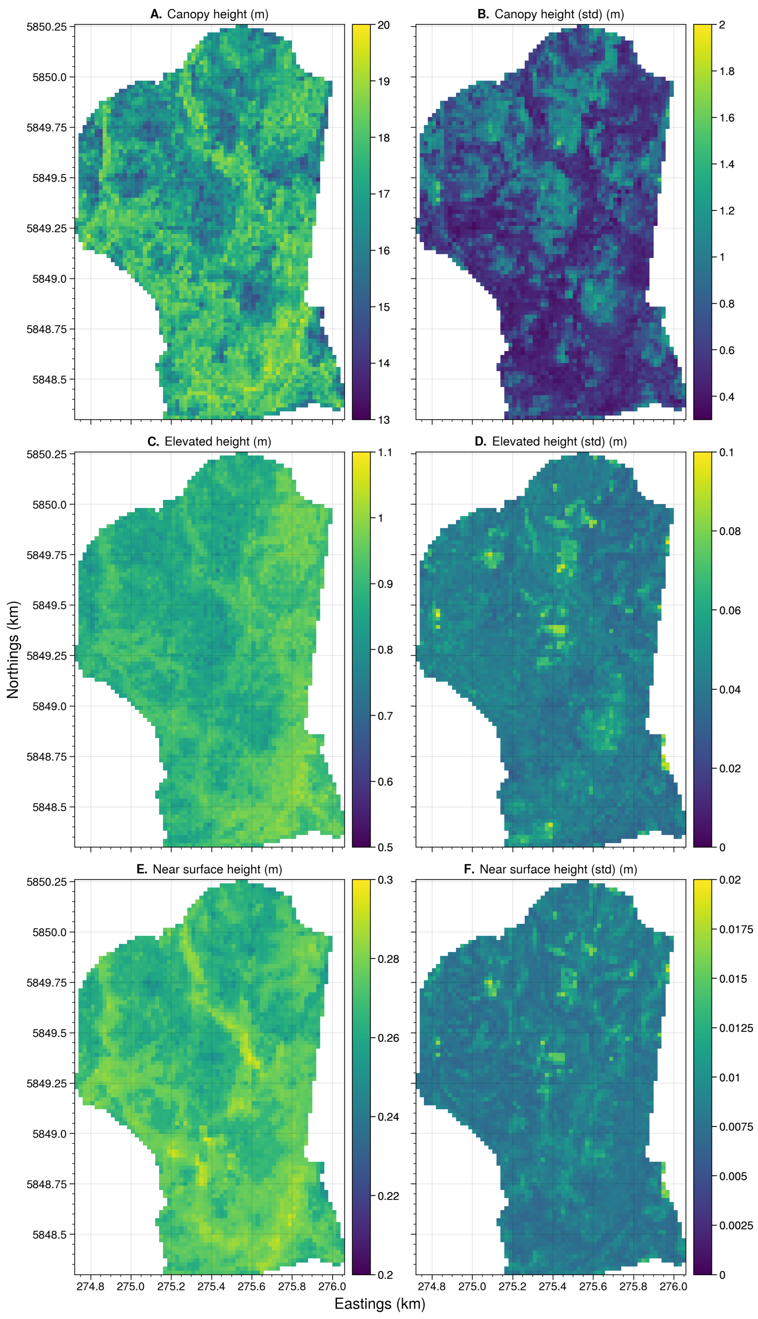
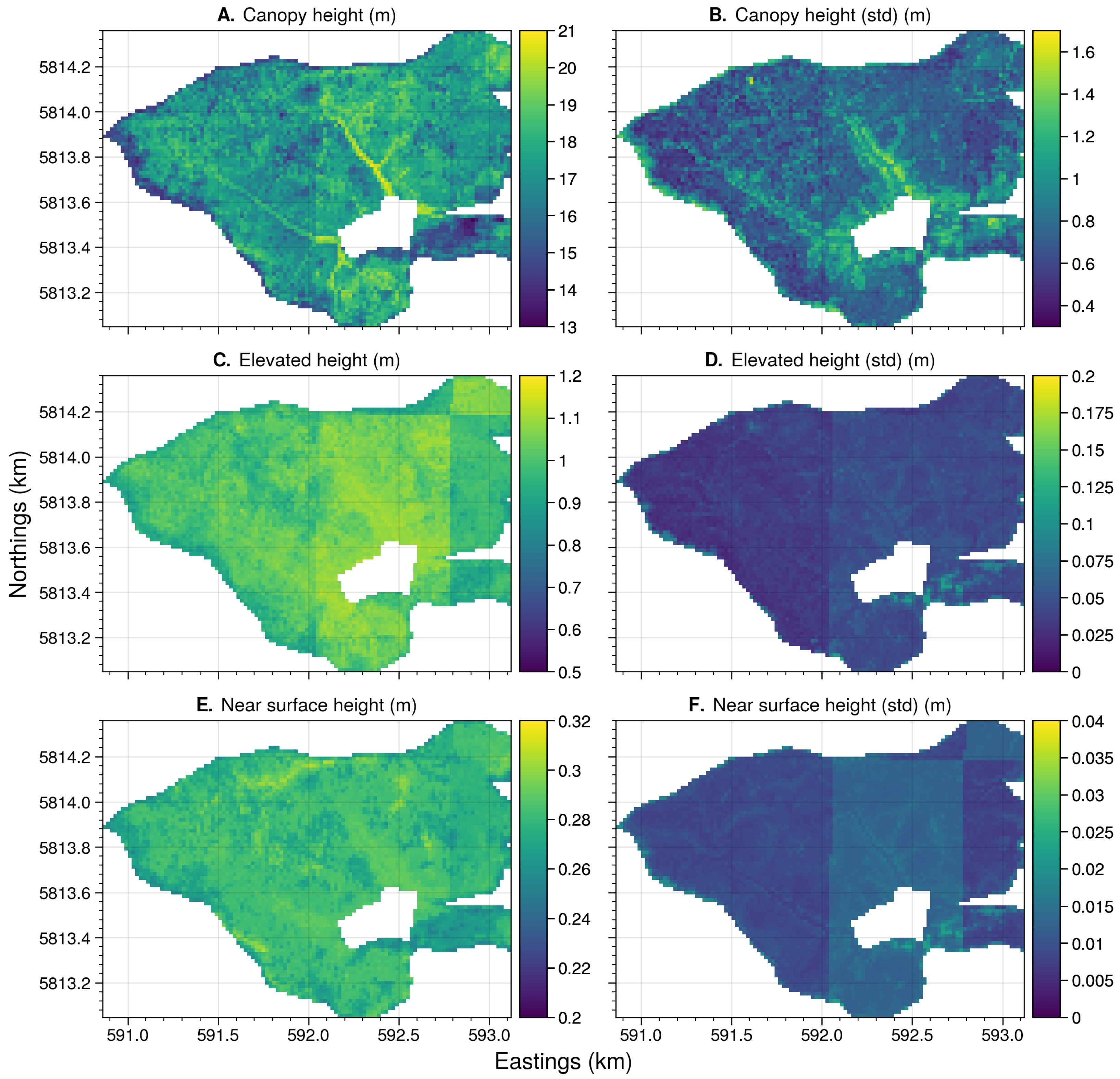
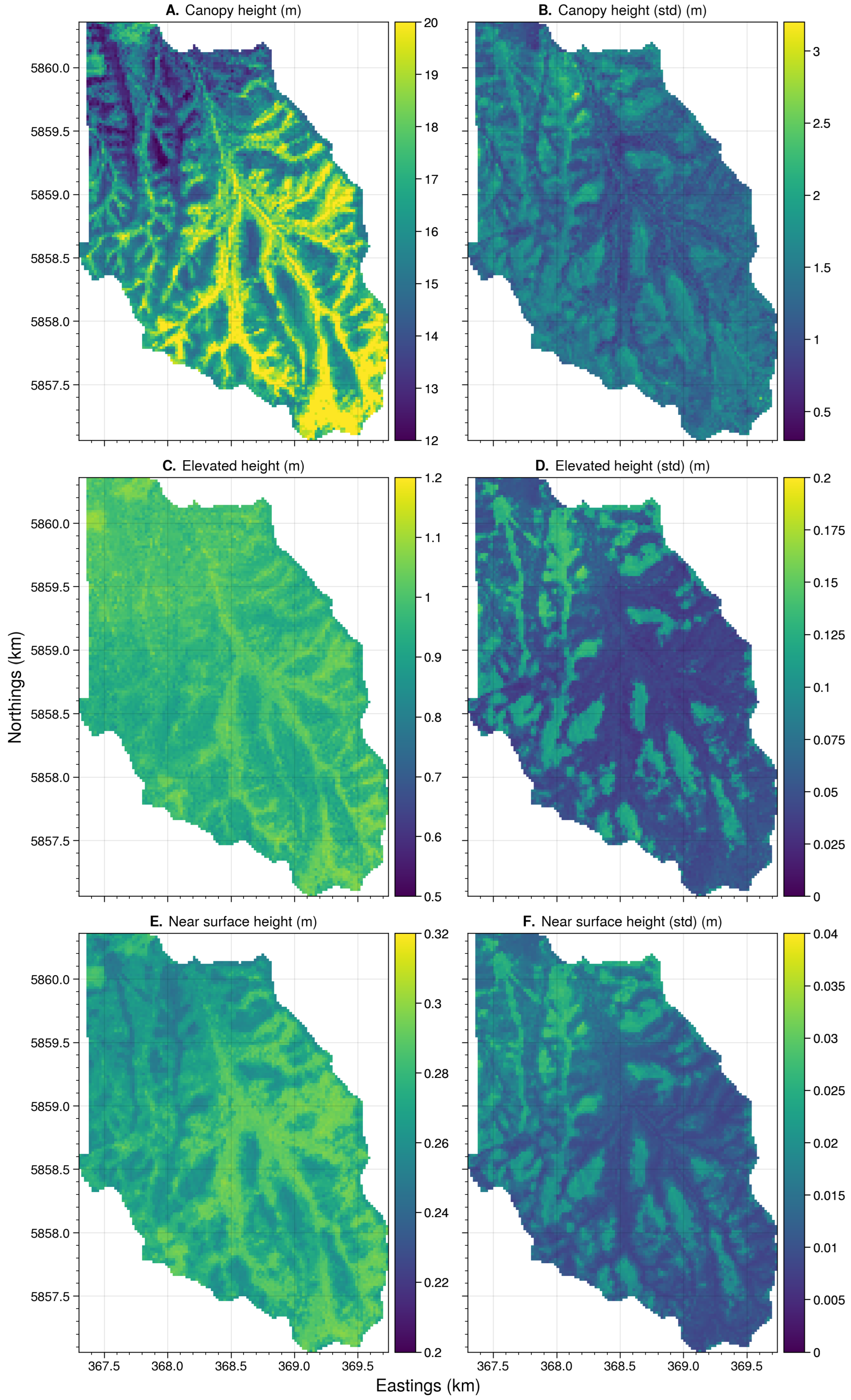
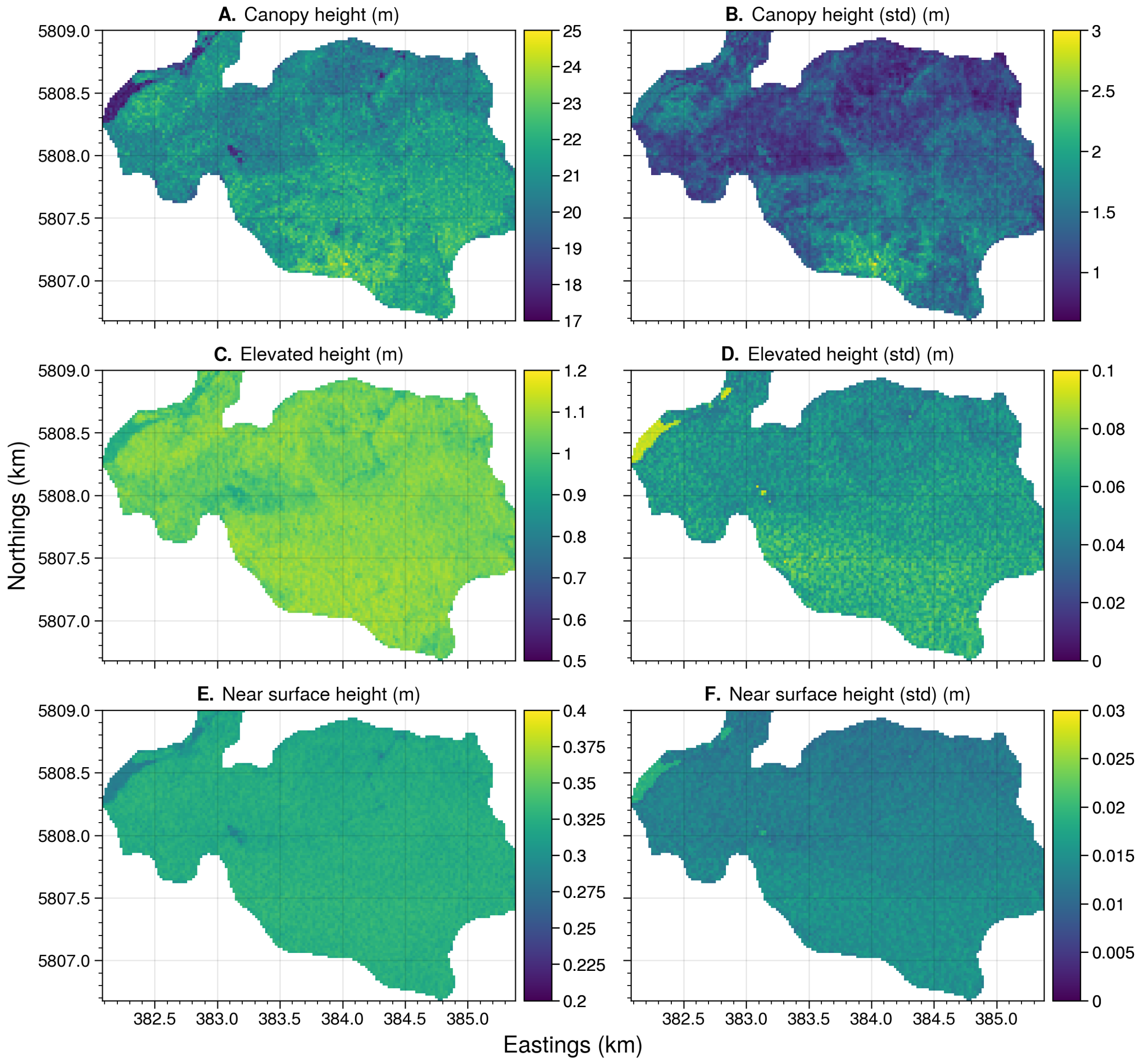
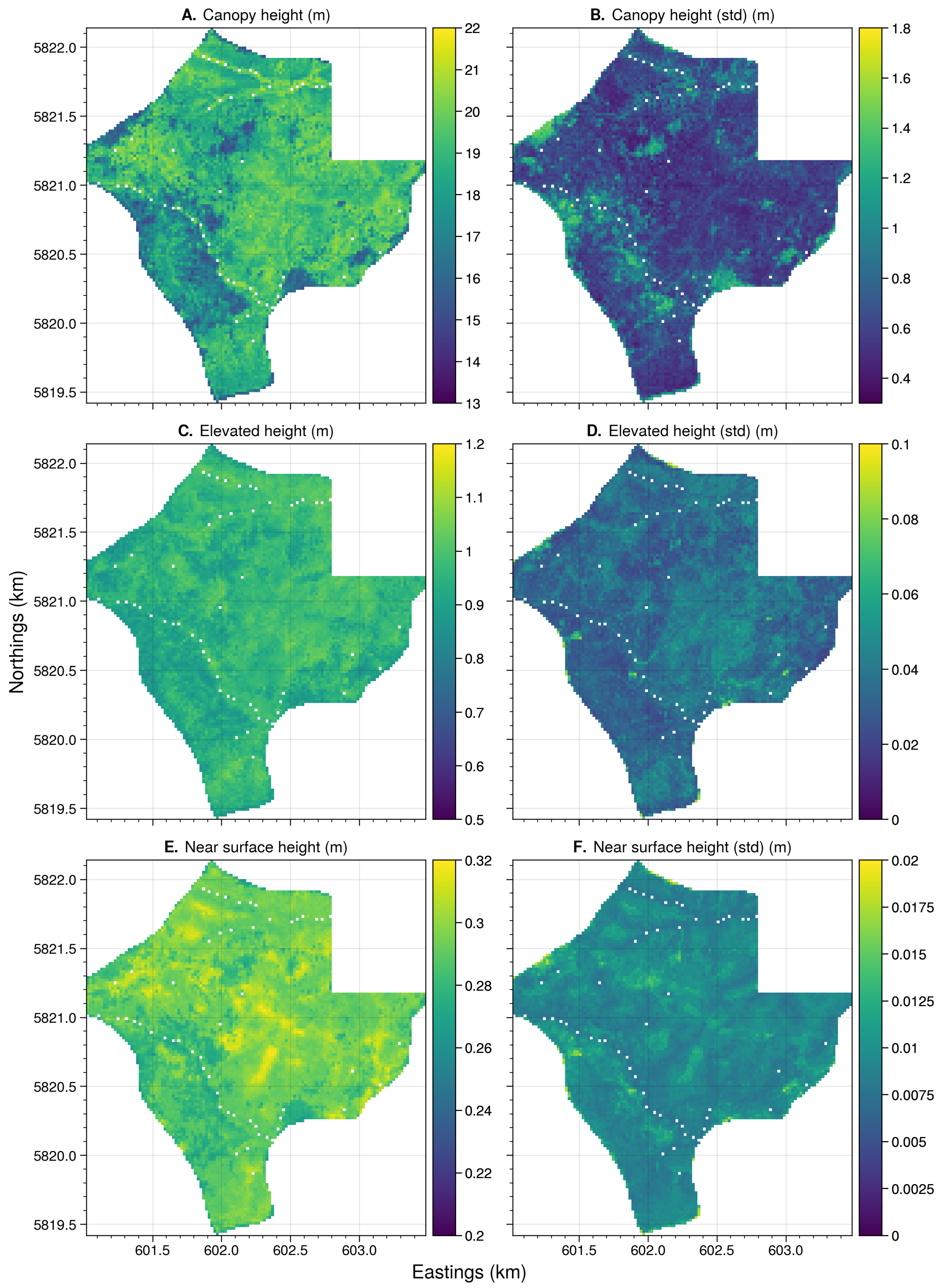
The TLS and visual assessment produced different magnitudes of cover within the near-surface and elevated layers, consistent with the differences seen in the comparison of infield data. Where the near-surface cover was higher and elevated cover was lower within the model predictions based on visual assessments, the TLS-based model predicted lower near-surface and higher elevated fuel cover (Figure 6). For example, at Clonbinane the mean near-surface cover predicted by the random forest model trained with TLS estimates was 34% in comparison to 55% from the random forest model trained with visual assessments (Figure 6). Despite being of differing magnitudes, similar landscape patterns of near-surface and elevated cover were predicted using the two training data inputs, as shown in Figure 7A,B and Figure 8A,B.

The standard deviation between the 100 predictions of cover for both the elevated and near-surface layer was lower across all seven sites when the TLS data were used to train the model (Figure 7C,D and Figure 8C,D) in comparison with when visual assessments were used to train the model. For example, the mean standard deviation of cover for the near-surface layer ranged from 2% (at Tostaree) to 3% (at Three Bridges) for TLS in comparison to 4% (at Tostaree) to 8% (at Three Bridges) for visual assessments. Patterns of standard deviation were similar between the predictions of the training data with higher variability in cover estimates occurring along the top of the slopes and the bottom of valleys. This is evident in Figure 7 and Figure 8 for Clonbinane and at all other sites (Appendix B). In both cases, the sites with a smaller number of plots in the area that was up-scaled produced higher variance in model estimates, suggesting that the conditions were not fully captured by the model. For example, where only four plots were used to up-scale an area of $482.7$ $\mathrm{h}\mathrm{a}$ (Three Bridges), a near-surface cover variance of 3.23% was produced, and where 14 plots were used to up-scale an area of $341.3$ $\mathrm{h}\mathrm{a}$ (Tostaree), a near-surface cover variance of 2% was produced (Figure 6).

4.4.2. Fuel Height

Landscape-level predictions of fuel height were also generated based on the TLS data (Figure 9 and figures in Appendix B). Similar features across the landscapes were observed in the height maps for both elevated and near-surface layer (Figure 9C,E). Patterns of standard deviation were also observed to be similar for both elevated and near-surface fuel height. This is evident in (Figure 9D,F) and at all other sites (figures related to height of fuel layers in Appendix B). The mean variation was observed to be low across the up-scaled area for both the near-surface and elevated layer for all seven sites (Figure 10).

Consistent features of landscape were observed in predicted maps of canopy height for all sites (Figure 9A and all figures in Appendix B). The mean variation in canopy height across the up-scaled areas for all seven sites was found to be low (<$1.4$ $\mathrm{m}$) (Figure 10). Relatively high variation in canopy height was observed in sites with low plot density (for instance, at Three Bridges ($1.34$ $\mathrm{m}$) where only four plots were used to up-scale an area of $482.7$ $\mathrm{h}\mathrm{a}$, the lowest variation ($0.7$ $\mathrm{m}$) in model prediction was observed at the Tostaree site, which had the highest plot density (Figure 10).

5. Discussion

The current visual approach to assess fuel hazard in southeast Australian forests provides a rapid means of assessing fuel and an indication of wildfire intensity. However, this approach has been shown to be subjective and does not provide a quantified estimate of fuel properties [30,31]. Nevertheless, using these data Jenkins et al. [15], McColl-Gausden et al. [27] demonstrated that environmental variables provide a driver of fuel hazard conditions across Victoria, Australia. In this study, the visually assessed fuel parameter estimates were captured followed Hines et al. [23] by the same set of observers over a short period of time. Despite this approach, removing some of the subjectivity associated with fuel hazard assessments, the random forest regression based on similar predictor variables to [15,27] failed to provide a prediction significantly improved over what could be achieved with random data. In comparison, moderate model performance was found when using TLS-derived properties for all metrics except for elevated fuel height. As such, in this study we demonstrated that the fuel properties derived from TLS data provide an improved source of plot-level data over visually assessed metrics for up-scaling fuel strata height and cover across the Victorian forests.

Previous attempts to describe landscape fuel conditions such as [15,27] based on plot-level visual assessments have often aimed to classify the landscape into fuel hazard classes (for instance, low, moderate, high, or extreme fuel hazard). By predicting classes, there is an inability to identify how certain classes were achieved. The workflow presented in this study provides an avenue for land managers to spatially interpolate metrics describing fuel properties by utilising observations from TLS. By predicting fuel properties instead of hazard, land managers are able to make informed decisions on how these properties may vary across the landscape without any loss of detail. To use these data to inform a fuel hazard rating, land managers may combine these products with live and dead fuel moisture readings as well observations of surface fuel hazard and bark hazard. Further research should be conducted to link non-morphological fuel characteristics with the structural metrics able to be derived from TLS to form a complete picture of the factors influencing fuel hazard.

The method used to randomly sample plot locations within the burn units in this study is currently implemented by Forest Fire Management Victoria staff and was developed to balance the capture of useful information and efficiency of data capture [76]. As such, plots were situated at least 100 $\mathrm{m}$ and no more than 500 $\mathrm{m}$ away from the road edge (to reduce edge effect whilst balancing human safety factors) with the number of plots scaled to the size of the burn unit. The determination of site placement did not consider changes in the landscape factors that are used to assist in the scaling-up of TLS data points. This likely caused the random forest predictions to fall within a narrower band than the overall fuel conditions at each location. Therefore, it is suggested that the method of sampling is refined, whereby further variables are added into the determination of the plot locations that are pertinent to the landscape measures able to be extracted from climate, soil, and satellite-derived datasets (e.g., the structurally guided sampling method [77]). By collecting data at sampling locations that are guided by environmental differences across the landscape (such as those highlighted in McColl-Gausden et al. [27]), it is likely that the location of plots spanning a greater range of fuel conditions will be obtained and in turn model accuracy estimates will likely improve.

In tandem with an improved sampling method, it is suggested that further variables to assist in the prediction of structural variables across the landscape are also considered. As highlighted in [15,26,27], the inclusion of time since fire and fire severity information from previous prescribed burning or wildfire is likely to assist in the prediction of structural metrics across an area. In this study, the plots captured did not show variability in time since fire, and hence this attribute was not used in the models. Satellite-based products have been shown to provide valuable information describing both the effect and recovery of Australian forests from disturbances [78,79,80,81]. The integration of such information to a modelling framework utilising plot-based TLS fuel properties will likely create greater understanding of fuel properties across a landscape as well as help in describing the dynamics of those properties.

Whilst the approach to process TLS point clouds shown here provides a more precise estimate of fuel properties than visual assessments, the produced results still require for decisions to be made for a number of metrics and thresholds. Using height thresholds to determine the attribution of vegetation elements to strata, for example, moves away from the physical description of fuel provided in Gould et al. [82], where fuel orientation (near-surface fuel is orientated horizontally, while elevated fuel is vertically orientated) should provide guidance as to the layer definition. By using defined height thresholds as in this research, negative correlation was seen between visual assessment and TLS methods. For example, where a dominant fuel element in a plot could be considered by an observer to be near-surface, due to its low height and orientation, the defined height threshold could result in this element being placed in the elevated layer during TLS processing. The consistent mapping of TLS-derived points (or point clusters) to physically relevant fuel strata remains a research challenge. Nevertheless, recent gains in areas such as in 3D machine learning point to potential improvements in the future processing of similar data [83]. However, further work is required to translate this into useful descriptions of fuel hazard.

It is vital that land and fire management staff further validate the products that are achieved using the method presented in this manuscript or similar approaches such as the one presented by Jenkins et al. [15], McColl-Gausden et al. [27]. Unlike the sole use of Airborne Laser Scanning data where land and fire managers can be completely remote from the production of fuel hazard metrics, sampling techniques such as terrestrial or mobile laser (MLS) scanning require on-ground sampling. Of these two technologies, it is believed that TLS is a preferred operational technique as it still provides a robust and repeatable measurement technique and requires the operator to remain in place for 3–5 min whilst each scan is undertaken [41,84]. This time provides the opportunity for the assessor to consider the plot area and capture ancillary information, such as photography of the site, and bark and surface fuel hazard assessments which are not currently able to be extracted from 3D point clouds. It is noted in a broader concept that landscape-specific sampling should be undertaken whereby if the landscape does not feature a dense forested canopy, ALS data may be sufficient to capture the fuel information required for a particular area [85,86].

6. Conclusions

This study presents a machine-learning-based method for estimating fuel metrics derived from TLS point clouds and visual assessment across an area relevant to operational fire management decisions. This method was applied across seven different sites distributed across Victoria, Australia. Plot-level data were collected by both TLS and visual assessments. The cover and height for three fuel layers such as near-surface, elevated, and canopy were derived from TLS point clouds. However, visual assessments were only available for cover of near-surface and elevated layers. Fuel metrics at landscape level were estimated by using a two-stage approach, firstly random forest models for each fuel metric were trained separately using TLS observations and visual assessments. Fuel metrics were then up-scaled to the large area by integrating topographic variables derived from ALS data, soil, climate variables, and vegetative indices derived from Sentinel MSI-2 imagery. The performance of a random forest model trained with TLS observation was compared with random forest models trained with visual assessment, where appropriate.

Our results show that the model trained and validated with TLS observations was found to have higher predictive power than the model trained with visual assessments for the cover of both fuel layers (near-surface and elevated). The results demonstrate the use of in-field TLS data coupled with machine learning approaches may provide a means to accurately generate fuel maps across the landscape and service operational decision-making as an alternative to visual-based assessments. The models utilising TLS data produced in this study could be utilised by fire managers to assess fuel treatment effectiveness and validate existing fuel maps. These results can be used to support a more robust determination of fuel metrics at the time of assessment and monitoring over time. The under-sampling of ranges and conditions was still found to be an issue with the TLS dataset as higher variation was observed in the cover and height for each fuel layer for those sites where a smaller number of plots were used for up-scaling larger areas. It is recommended that the sampling strategy should ultimately be driven according to the environmental differences across the landscape so that the location of plots cover a greater range of fuel conditions which in turn can improve the accuracy of the model.

References

1. Balch, J.; Bradley, B.; Abatzogloue, J.; Nagy, R.; Fuscod, E.; Mahood, A. Human-started wildfires expand the fire niche acrossthe United States. Environ. Sci. Sustain. Sci. 2017, 114, 2946–2951. [Google Scholar]
2. Cattau, M.; Wessman, C.; Mahood, A.; Balch, J. Anthropogenic and lightning-started fires are becoming larger and more frequent over a longer season length in the U.S.A. Glob. Ecol. Biogeogr. 2020, 29, 668–681. [Google Scholar] [CrossRef]
3. Liu, M.; Yang, L. Human-caused fires release more carbon than lightning-caused fires in the conterminous United States. Environ. Res. Lett. 2020, 16, 014013. [Google Scholar] [CrossRef]
4. Duane, A.; Castellnou, M.; Brotons, L. Towards a comprehensive look at global drivers of novel extreme wildfire events. Clim. Chang. 2021, 165, 43. [Google Scholar] [CrossRef]
5. Nauslar, N.; Abatzoglou, J.; Marsh, P. The 2017 North Bay and Southern California Fires: A case study. Fire 2018, 1, 18. [Google Scholar] [CrossRef] [Green Version]
6. Porter, T.W.; Crowfoot, W.; Newsom, G. Wildfire Activity Statistics; California Department of Forestry and Fire Protection: Sacramento, CA, USA, 2019. Available online: https://www.fire.ca.gov/incidents/2019 (accessed on 17 November 2022).
7. Coogan, S.; Robinne, F.; Jain, P.; Flannigan, M. Scientists’ warning on wildfire—A Canadian perspective. Can. J. For. Res. 2019, 49, 1015–1023. [Google Scholar] [CrossRef] [Green Version]
8. Munawar, H.; Ullah, F.; Khan, S.; Qadir, Z.; Qayyum, S. UAV assisted spatiotemporal analysis and management of bushfires: A case study of the 2020 Victorian Bushfires. Fire 2021, 4, 40. [Google Scholar] [CrossRef]
9. Cruz, M.; Cheney, N.; Gould, J.; McCaw, W.; Kilinc, M.; Sullivan, A. An empirical-based model for predicting the forward spread rate of wildfires in eucalypt forests. Int. J. Wildland Fire 2022, 31, 81–95. [Google Scholar] [CrossRef]
10. Linn, R.; Goodrick, S.; Brown, M.; Middleton, R.; OBrien, J.; Hiers, J. QUIC-fire: A fast-running simulation tool for prescribed fire planning. Environ. Model. Softw. 2020, 125, 104616. [Google Scholar] [CrossRef]
11. Miller, C.; Hilton, J.; Sullivan, A.; Prakash, M. SPARK—A bushfire spread prediction tool. IFIP Adv. Inf. Commun. Technol. 2015, 448, 262–271. [Google Scholar]
12. Taneja, R.; Hilton, J.; Wallace, L.; Reinke, K.; Jones, S. Effect of fuel spatial resolution on predictive wildfire models. Int. J. Wildland Fire 2021, 30, 776–789. [Google Scholar] [CrossRef]
13. Cruz, M.; McCaw, W.; Anderson, W.; Gould, J. Fire behavior modelling in semi-arid Mallee-heath shrublands of southern Australia. Environ. Model. Softw. 2013, 40, 21–34. [Google Scholar] [CrossRef]
14. Fernandes, P.M.; Botelho, H.S. A review of prescribed burning effectiveness in fire hazard reduction. Int. J. Wildland Fire 2003, 12, 117–128. [Google Scholar] [CrossRef] [Green Version]
15. Jenkins, M.E.; Bedward, M.; Price, O.; Bradstock, R.A. Modelling bushfire fuel hazard using biophysical parameters. Forests 2020, 11, 925. [Google Scholar] [CrossRef]
16. Thompson, M.; Vaillant, N.; Hass, J.; Gebert, K. Modelling surface fine fuel dynamics across climate gradients in eucalypt forests of south-eastern Australia. J. For. 2013, 111, 49–58. [Google Scholar]
17. Catchpole, W.; Wheeler, C. Estimating plant biomass: A review of techniques. Aust. J. Ecol. 1992, 17, 121–131. [Google Scholar] [CrossRef]
18. Price, O.; Gordon, C. The potential for LiDAR technology to map fire fuel hazard over large areas of australian forest. J. Environ. Manag. 2016, 181, 663–673. [Google Scholar] [CrossRef] [PubMed]
19. Van Wagner, C. The line intersect method in forest fuel sampling. For. Sci. 1968, 14, 20–26. [Google Scholar]
20. Elshikha, D. Using RGB-based vegetation indices for monitoring guayule biomass, moisture content and rubber. In Proceedings of the ASABE Annual International Meeting, Orlando, FL, USA, 17–20 July 2016. [Google Scholar]
21. Rowell, E.; Loudermilk, E.L.; Hawley, C.; Pokswinski, S.; Seielstad, C.; Queen, L.; O’Brien, J.J.; Hudak, A.T.; Goodrick, S.; Hiers, J.K. Coupling terrestrial laser scanning with 3D fuel biomass sampling for advancing wildland fuels characterization. For. Ecol. Manag. 2020, 462, 117945. [Google Scholar] [CrossRef]
22. Loudermilk, E.; Hiers, J.; O’Brien, J.; Mitchell, R.; Singhania, A.; Fernandez, J.; Cropper, W.; Slatton, K. Ground-based LiDAR: A novel approach to quantify fine-scale fuelbed characteristics. Int. J. Wildland Fire 2009, 18, 676–685. [Google Scholar] [CrossRef] [Green Version]
23. Hines, F.; Tolhurst, K.G.; Wilson, A.A.G.; McCarthy, G.J. Overall Fuel Hazard Assessment Guide, 4th ed.; Victorian Government, Department of Sustainability and Environment: East Melbourne, Australia, 2010; Volume 82, pp. 1–41.
24. 24.Prichard, S.J.; Sandberg, D.V.; Ottmar, R.D.; Eberhardt, E.; Andreu, A.; Eagle, P.; Swedin, K. Fuel Characteristic Classification System Version 3.0: Technical Documentation; Gen. Tech. Rep. PNW-GTR-887; US Department of Agriculture, Forest Service, Pacific Northwest Research Station: Portland, OR, USA, 2013; Volume 887, 79p.
25. Prichard, S.J.; Andreu, A.G.; Ottmar, R.D.; Eberhardt, E. Fuel Characteristic Classification System (FCCS) Field Sampling and Fuelbed Development Guide; Gen. Tech. Rep. PNW-GTR-972; U.S. Department of Agriculture, Forest Service, Pacific Northwest Research Station: Portland, OR, USA, 2019; p. 77.
26. Duff, T.J.; Bell, T.L.; York, A. Predicting continuous variation in forest fuel load using biophysical models: A case study in south-eastern Australia. Int. J. Wildland Fire 2012, 22, 318–332. [Google Scholar] [CrossRef]
27. McColl-Gausden, S.; Bennett, L.; Duff, T.; Cawson, J.; Penman, T. Climatic and edaphic gradients predict variation in wildland fuel hazard in south-eastern Australia. Ecography 2020, 43, 443–455. [Google Scholar] [CrossRef] [Green Version]
28. Penman, T.; McColl-Gausden, S.; Cirulis, B.; Kultaev, D.; Bennett, L. Improved accuracy of wildfire simulations using fuel hazard estimates based on environmental data. J. Environ. Manag. 2022, 301, 113789. [Google Scholar] [CrossRef]
29. Gosper, C.R.; Yates, C.J.; Prober, S.M.; Wiehl, G. Application and validation of visual fuel hazard assessments in dry Mediterranean-climate woodlands. Int. J. Wildland Fire 2014, 23, 385. [Google Scholar] [CrossRef] [Green Version]
30. Spits, C.; Wallace, L.; Reinke, K. Investigating Surface and Near-Surface Bushfire Fuel Attributes: A Comparison between Visual Assessments and Image-Based Point Clouds. Sensors 2017, 17, 910. [Google Scholar] [CrossRef] [Green Version]
31. Watson, P.J.; Penman, S.H.; Bradstock, R.A. A comparison of bushfire fuel hazard assessors and assessment methods in dry sclerophyll forest near Sydney, Australia. Int. J. Wildland Fire 2012, 21, 755–763. [Google Scholar] [CrossRef]
32. Gajardo, J.; García, M.; Riaño, D. Applications of airborne laser scanning in forest fuel assessment and fire prevention. In Forestry Applications of Airborne Laser Scanning; Springer: Berlin/Heidelberg, Germany, 2014; pp. 439–462. [Google Scholar] [CrossRef]
33. Lovell, J.L.; Jupp, D.L.; Culvenor, D.S.; Coops, N.C. Using airborne and ground-based ranging LiDAR to measure canopy structure in Australian forests. Can. J. Remote Sens. 2003, 29, 607–622. [Google Scholar] [CrossRef]
34. Hilker, T.; Coops, N.C.; Newnham, G.J.; van Leeuwen, M.; Wulder, M.A.; Stewart, J.; Culvenor, D.S. Comparison of Terrestrial and Airborne LiDAR in Describing Stand Structure of a Thinned Lodgepole Pine Forest. J. For. 2012, 110, 97–104. [Google Scholar] [CrossRef]
35. Calders, K.; Adams, J.; Armston, J.; Bartholomeus, H.; Bauwens, S.; Bentley, L.P.; Chave, J.; Danson, F.M.; Demol, M.; Disney, M.; et al. Terrestrial laser scanning in forest ecology: Expanding the horizon. Remote Sens. Environ. 2020, 251, 112102. [Google Scholar] [CrossRef]
36. Gupta, V.; Reinke, K.; Jones, S.; Wallace, L.; Holden, L. Assessing Metrics for Estimating Fire Induced Change in the Forest Understorey Structure Using Terrestrial Laser Scanning. Remote Sens. 2015, 7, 8180–8201. [Google Scholar] [CrossRef] [Green Version]
37. Hillman, S.; Wallace, L.; Reinke, K.; Jones, S. A comparison between TLS and UAS LiDAR to represent eucalypt crown fuel characteristics. ISPRS J. Photogramm. Remote Sens. 2021, 181, 295–307. [Google Scholar] [CrossRef]
38. Hudak, A.; Bright, B.; Rowell, E.; Robertson, K.; Pokswinski, S.; Hiers, K.; Prichard, S.; Nowell, H.; Holmes, C.; Gargulinski, E.; et al. Estimating Surface Fuel Density from TLS and ALS: A Two-Tiered Approach that Accounts for Sampling Scale. In Proceedings of the SilviLaser Conference, Vienna, Austria, 28–30 September 2021; pp. 123–125. [Google Scholar]
39. Levick, S.R.; Whiteside, T.; Loewensteiner, D.A.; Rudge, M.; Bartolo, R. Leveraging TLS as a Calibration and Validation Tool for MLS and ULS Mapping of Savanna Structure and Biomass at Landscape-Scales. Remote Sens. 2021, 13, 257. [Google Scholar] [CrossRef]
40. Pokswinski, S.; Gallagher, M.R.; Skowronski, N.S.; Loudermilk, E.L.; Hawley, C.; Wallace, D.; Everland, A.; Wallace, J.; Hiers, J.K. A simplified and affordable approach to forest monitoring using single terrestrial laser scans and transect sampling. MethodsX 2021, 8, 101484. [Google Scholar] [CrossRef] [PubMed]
41. Wallace, L.; Hillman, S.; Hally, B.; Taneja, R.; McGlade, J. Terrestrial Laser Scanning: An Operational Tool for Fuel Hazard Mapping? Fire 2022, 5, 85. [Google Scholar] [CrossRef]
42. Muir, J.; Phinn, S.; Eyre, T.; Scarth, P. Measuring plot scale woodland structure using terrestrial laser scanning. Remote Sens. Ecol. Conserv. 2018, 4, 320–338. [Google Scholar] [CrossRef] [Green Version]
43. Newnham, G.J.; Armston, J.D.; Calders, K.; Disney, M.I.; Lovell, J.L.; Schaaf, C.B.; Strahler, A.H.; Danson, F.M. Terrestrial laser scanning for plot-scale forest measurement. Curr. For. Rep. 2015, 1, 239–251. [Google Scholar] [CrossRef] [Green Version]
44. State Government of Victoria. Fuel Management Report 2020–21: Statewide Outcomes and Delivery-Victorian Bushfire Monitoring Program; State Government of Victoria: Melbourne, Australia, 2021.
45. Cartus, O.; Kellndorfer, J.; Rombach, M.; Walker, W. Mapping canopy height and growing stock volume using airborne LiDAR, ALOS PALSAR and Landsat ETM+. Remote Sens. 2012, 4, 3320–3345. [Google Scholar] [CrossRef] [Green Version]
46. Wilkes, P.; Jones, S.D.; Suarez, L.; Mellor, A.; Woodgate, W.; Soto-Berelov, M.; Haywood, A.; Skidmore, A.K. Mapping Forest Canopy Height Across Large Areas by Upscaling ALS Estimates with Freely Available Satellite Data. Remote Sens. 2015, 7, 12563–12587. [Google Scholar] [CrossRef] [Green Version]
47. Armston, J.; Denham, R.; Danaher, T.; Scarth, P.; Moffiet, T. Prediction and validation of foliage projective cover from Landsat-5 TM and Landsat-7 ETM+. J. Appl. Remote Sens. 2009, 3, 033540. [Google Scholar] [CrossRef]
48. Leite, R.; Silva, C.; Broadbent, E.; Amaral, C.; Liesenberg, V.; Almeida, D.; Mohan, M.; Godinho, S.; Cardil, A.; Hamamura, C.; et al. Large scale multi-layer fuel load characterization in tropical savanna using GEDI spaceborne LiDAR data. Remote Sens. Environ. 2022, 268, 112764. [Google Scholar] [CrossRef]
49. D’Este, M.; Elia, M.; Vincenzo, G.; Giuseppina, S.; Raffaele, L.; Giovanni, S. Machine Learning Techniques for Fine Dead Fuel Load Estimation Using Multi-Source Remote Sensing Data. Remote Sens. 2021, 13, 1658. [Google Scholar] [CrossRef]
50. Lau, A.; Bentley, L.; Martius, C. Quantifying branch architecture of tropical trees using terrestrial LiDAR and 3D modelling. Int. J. Wildland Fire 2018, 32, 1219–1231. [Google Scholar] [CrossRef] [Green Version]
51. Ashcroft, M.; Gollan, J.; Ramp, D. Creating vegetation density profiles for a diverse range of ecological habitats using terrestrial laser scanning methods. Ecol. Evol. 2014, 5, 263–272. [Google Scholar]
52. Palace, M.; Sullivan, F.; Ducey, M.; Herrick, C. Estimating tropical forest structure using a terrestrial LiDAR. PLoS ONE 2016, 11, e0154115. [Google Scholar] [CrossRef] [PubMed] [Green Version]
53. Chen, H.; Zhu, X.; Yebra, M.; Harris, S.; Tapper, N. Strata-based forest fuel classification for wild fire hazard assessment using terrestrial LiDAR. J. Appl. Remote Sens. 2016, 10, 046025. [Google Scholar] [CrossRef] [Green Version]
54. Hudak, A.; Evans, J.; Stuart Smith, A. LiDAR utility for natural resource managers. Remote Sens. 2009, 1, 934–951. [Google Scholar] [CrossRef] [Green Version]
55. Vosselman, G.; Gorte, B.; Sithole, G. Recognising strucutre in laser scanner point clouds. Remote Sens. Spat. Inf. Sci. 2004, 32, 33–38. [Google Scholar]
56. Rusu, R.B.; Marton, Z.C.; Blodow, N.; Dolha, M.; Beetz, M. Towards 3D Point cloud based object maps for household environments. Robot. Auton. Syst. 2008, 56, 927–941. [Google Scholar] [CrossRef]
57. Zhang, W.; Qi, J.; Wan, P.; Wang, H.; Xie, D.; Wang, X.; Yan, G. An easy-to-use airborne LiDAR data filtering method based on cloth simulation. Remote Sens. 2016, 8, 501. [Google Scholar] [CrossRef]
58. Gould, J.S.; Lachlan McCaw, W.; Phillip Cheney, N. Quantifying fine fuel dynamics and structure in dry eucalypt forest (Eucalyptus marginata) in Western Australia for fire management. For. Ecol. Manag. 2011, 262, 531–546. [Google Scholar] [CrossRef]
59. Pedregosa, F.; Varoquaux, G.; Gramfort, A.; Michel, V.; Thirion, B.; Grisel, O.; Blondel, M.; Prettenhofer, P.; Weiss, R.; Dubourg, V.; et al. Scikit-learn: Machine Learning in Python. J. Mach. Learn. Res. 2011, 12, 2825–2830. [Google Scholar]
60. Linusson, H. Multi-Output Random Forests. Master’s Thesis, University of Borås, Borås, Sweden, 2013. [Google Scholar]
61. Yadav, B.K.V.; Lucieer, A.; Jordan, G.J.; Baker, S.C. Using topographic attributes to predict the density of vegetation layers in a wet eucalypt forest. Aust. For. 2022, 85, 25–37. [Google Scholar] [CrossRef]
62. Hageer, Y.; Esperón-Rodríguez, M.; Baumgartner, J.B.; Beaumont, L.J. Climate, soil or both? Which variables are better predictors of the distributions of Australian shrub species? PeerJ 2017, 5, e3446. [Google Scholar] [CrossRef] [PubMed]
63. DeCastro, A.; Juliano, T.; Kosović, B.; Ebrahimian, H.; Balch, J. A computationally efficient Method for Updating Fuel Inputs for Wildfire Behavior Models Using Sentinel Imagery and Random Forest Classification. Remote Sens. 2022, 14, 1447. [Google Scholar] [CrossRef]
64. Hudak, A.T.; Kato, A.; Bright, B.C.; Loudermilk, E.L.; Hawley, C.; Restaino, J.C.; Ottmar, R.D.; Prata, G.A.; Cabo, C.; Prichard, S.J.; et al. Towards Spatially Explicit Quantification of Pre- and Postfire Fuels and Fuel Consumption from Traditional and Point Cloud Measurements. For. Sci. 2020, 66, 428–442. [Google Scholar] [CrossRef]
65. Meddens, A.; Hicke, J.; Vierling, L.; Hudak, A. Evaluating methods to detect bark beetle-caused tree mortality using single-date and multi-date Landsat imagery. Remote Sens. Environ. 2013, 132, 49–58. [Google Scholar] [CrossRef]
66. Wang, B.; Zhang, G.; Duan, J. Relationship between topography and the distribution of understory vegetation in a Pinus massoniana forest in Southern China. Int. Soil Water Conserv. Res. 2015, 3, 291–304. [Google Scholar] [CrossRef] [Green Version]
67. Viscarra Rossel, R.; Chen, C.; Grundy, M.; Searle, B.; Clifford, D.; Campbell, P. The Australian three-dimensional soil grid: Australia’s contribution to the GlobalSoilMap project. Soil Res. 2015, 53, 845–864. [Google Scholar] [CrossRef] [Green Version]
68. Fick, S.; Hijmans, R. WorldClim 2: New 1km spatial resolution climate surfaces for global land areas. Int. J. Climatol. 2017, 37, 4302–4315. [Google Scholar] [CrossRef]
69. Breiman, L. Bagging predictors. Machine Learning. Mach. Learn. 1996, 24, 123–140. [Google Scholar] [CrossRef] [Green Version]
70. Qian, W.; Yang, Y.; Zou, H. Tweedie’s compound poisson model with grouped elastic net. J. Comput. Graph. Stat. 2016, 25, 606–625. [Google Scholar] [CrossRef]
71. Yang, Y.; Qian, W.; Zou, H. Insurance premium prediction via gradient tree-boosted tweedie compound poisson models. J. Bus. Econ. Stat. 2018, 36, 456–470. [Google Scholar] [CrossRef] [Green Version]
72. Freeman, E.; Moisen, G.; Coulston, J.; Wilson, B. Random forests and stochastic gradient boosting for predicting tree canopy cover: Comparing tuning processes and model performance. Can. J. For. Res. 2015, 46, 323–339. [Google Scholar] [CrossRef] [Green Version]
73. Fletcher, R.S. Using Vegetation Indices as Input into Random Forest for Soybean and Weed Classification. Am. J. Plant Sci. 2016, 7, 2186–2198. [Google Scholar] [CrossRef] [Green Version]
74. Gao, Y.; Lu, D.; Li, G.; Wang, G.; Chen, Q.; Liu, L.; Li, D. Comparative analysis of modeling algorithms for forest aboveground biomass estimation in a subtropical region. Remote Sens. 2018, 10, 627. [Google Scholar] [CrossRef] [Green Version]
75. Rocha, A.; Groen, T.; Skidmore, A.; Darvishzadeh, R.; Willemen, L. Machine learning using hyperspectral data inaccurately predicts plant traits under spatial dependency. Remote Sens. 2018, 10, 1263. [Google Scholar] [CrossRef] [Green Version]
76. State Government of Victoria. Monitoring, Evaluation and Reporting Framework for Bushfire Management on Public Land; State Government of Victoria: Melbourne, Australia, 2015.
77. Goodbody, T.R.H.; Coops, N.C.; Queinnec, M.; White, J.C.; Tompalski, P.; Hudak, A.T.; Auty, D.; Valbuena, R.; LeBoeuf, A.; Sinclair, I.; et al. sgsR: A structurally guided sampling toolbox for LiDAR-based forest inventories. For. Int. J. Forest Res. 2023, cpac055. [Google Scholar] [CrossRef]
78. Massetti, A.; Rüdiger, C.; Yebra, M.; Hilton, J. The Vegetation Structure Perpendicular Index (VSPI): A forest condition index for wildfire predictions. Remote Sens. Environ. 2019, 224, 167–181. [Google Scholar] [CrossRef]
79. Chhabra, A.; Rüdiger, C.; Yebra, M.; Jagdhuber, T.; Hilton, J. RADAR-Vegetation Structural Perpendicular Index (R-VSPI) for the Quantification of Wildfire Impact and Post-Fire Vegetation Recovery. Remote Sens. 2022, 14, 3132. [Google Scholar] [CrossRef]
80. Collins, L.; Griffioen, P.; Newell, G.; Mellor, A. The utility of Random Forests for wildfire severity mapping. Remote Sens. Environ. 2018, 216, 374–384. [Google Scholar] [CrossRef]
81. Gibson, R.K.; White, L.A.; Hislop, S.; Nolan, R.H.; Dorrough, J. The post-fire stability index; a new approach to monitoring post-fire recovery by satellite imagery. Remote Sens. Environ. 2022, 280, 113151. [Google Scholar] [CrossRef]
82. Gould, J.S.; McCaw, W.; Cheney, N.; Ellis, P.; Knight, I.; Sullivan, A. Project Vesta: Fire in Dry Eucalypt Forest: Fuel Structure, Fuel Dynamics and Fire Behaviour; CSIRO Publishing: Clayton, Australia, 2008. [Google Scholar]
83. Krisanski, S.; Taskhiri, M.S.; Aracil, G.; Muneri, A.; Gurung, M.B.; Montgomery, J.; Turner, P. Forest Structural Complexity Tool—An Open Source, Fully-Automated Tool for Measuring Forest Point Clouds. Remote Sens. 2021, 13, 4677. [Google Scholar] [CrossRef]
84. Bienert, A.; Georgi, L.; Kunz, M.; Maas, H.; Oheimb, G. Comparison and Combination of Mobile and Terrestrial Laser Scanning for Natural Forest Inventories. Forests 2018, 9, 395. [Google Scholar] [CrossRef] [Green Version]
85. William, W.; Mariela, S.B.; Lola, S.; Simon D., J.; Michael, H.; Phil, W.; Christoffer, A.; Andrew, H.; Andrew, M. Searching for the Optimal Sampling Design for Measuring LAI in an Upland Rainforest. In Proceedings of the Geospatial Science Research Symposium GSR2, Melbourne, Australia, 10–12 December 2012. [Google Scholar]
86. EPA Technical Guidance—Flora and Vegetation Surveys for Environmental Impact Assessment; Technical Report; EPA: Joondalup, Australia, 2016.
87. Travis, M.; Elsner, G.; Iverson, W.; Jonnson, C. VIEWIT: Computation of Seen Areas, Slope, and Aspect for Landuse Planning; Department of Agriculture, Forest Service, Pacific Southwest Forest and Range Experiment Station: Berkeley, CA, USA, 1975.
88. Kiss, R. Determination of drainage network in digital elevation models, utilities and limitations. J. Hung. Geomath. 2004, 2, 16–29. [Google Scholar]
89. Wilson, M.; O’Connell, B.; Brown, C.; Guinan, J.; Grehan, A. Multiscale terrain analysis of multibeam bathymetry data for habitat mapping on the continental slope. Mar. Geodesy. 2007, 30, 3–35. [Google Scholar] [CrossRef] [Green Version]
90. Lukovic, J.; Bajat, B.; Kilibarda, M.; Filipovic, D. High resolution grid of potential incoming solar radiation for Serbia. Therm. Sci. 2015, 19, s427–s435. [Google Scholar] [CrossRef]
91. De Reu, J.; Bourgeois, J.; Bats, M.; Zwertvaegher, A.; Gelorini, V.; De Smedt, P.; Chu, W.; Antrop, M.; De Maeyer, P.; Finke, P. Application of the topographic position index to heterogeneous landscapes. Geomorphology 2013, 186, 39–49. [Google Scholar] [CrossRef]
92. Riley, S.; Stephen, D.; Elliot, R. A terrain ruggedness index that quantifies topographic heterogeneity. Int. J. Sci. 1999, 5, 23–27. [Google Scholar]
93. Jacoby, B.; Peterson, E.; Dogwiler, T. Identifying the stream erosion potential of cave levels in Carter Cave State Resort Park, Kentucky, USA. J. Geogr. Inf. Syst. 2011, 3, 323–333. [Google Scholar] [CrossRef] [Green Version]
94. Sørensen, R.; Zinko, U.; Seibert, J. On the calculation of the topographic wetness index: Evaluation of different methods based on field observations. Hydrol. Earth Syst. Sci. 2006, 10, 101–112. [Google Scholar] [CrossRef] [Green Version]
95. O’Donnell, M.; Ignizio, D. Bioclimatic Predictors for Supporting Ecological Applications in the Conterminous United States; U.S. Geological Survey: Reston, VA, USA, 2012; p. 10.
96. Weier, J.; Herring, D. Measuring Vegetation (NDVI & EVI); NASA Earth Observatory: Washington, DC, USA, 2000.
97. Nedkov, R. Orthogonal transformation of segmented images from the satellite Sentinel-2. Comptes Rendus L’acad. Bulg. Sci. 2017, 70, 687–692. [Google Scholar]
98. Gitelson, A.; Gritz, Y.; Merzlyak, M. Relationships between leaf chlorophyll content and spectral reflectance and algorithms for non-destructive chlorophyll assessment in higher plant leaves. J. Plant Physiol. 2003, 160, 271–282. [Google Scholar] [CrossRef] [PubMed]
99. Gitelson, A.; Gritz, Y.; Merzlyak, M. Three-band model for noninvasive estimation of chlorophyll, carotenoids, and anthocyanin contents in higher plant leaves. Geophys. Res. Lett. 2006, 33, L11402. [Google Scholar] [CrossRef] [Green Version]
Figure 1. (a) The location of the seven study sites in Victoria, Australia. Photos of typical conditions at the (b) Bullengarook (S1), (c) Clonbinane (S2), (d) Lakes Entrance (S3), (e) Murrindindi (S4), (f) Three Bridges (S5), (g) Toorloo Arm (S6), and (h) Tostaree (S7) sites.
Remotesensing 15 01273 g001
Figure 2. The workflow used to generate prediction of fuel properties (near-surface and elevated fuel cover and height) for the extent of an area that needed to be up-scaled.
Remotesensing 15 01273 g002
Figure 3. Joint plots comparing cover (%) for the (A) near-surface and (B) elevated fuel layers from TLS and visually assessed (VA) observations.
Remotesensing 15 01273 g003
Figure 4. Joint plots comparing cover (%) of the near-surface (A,B) and elevated (C,D) layers. (A,C) show the TLS observation against the random forest prediction (trained using TLS data). (B,D) show the visually assessed cover against the random forest prediction (trained using visually assessed data).
Remotesensing 15 01273 g004
Figure 5. Joint plots showing fuel height observed using TLS point clouds and mean prediction from the random forest models trained with TLS observations for (A) near-surface (B) elevated (C) canopy fuel layers.
Remotesensing 15 01273 g005
Figure 6. Box plots showing comparison between mean prediction of cover (%) from the random forest models trained with TLS observations and mean prediction from the random forest models trained with visual assessments for (A) near-surface and (B) elevated layers.
Remotesensing 15 01273 g006
Figure 7. The mean and standard deviation of landscape level predictions for elevated fuel cover using visual assessments (A,C) and TLS (B,D) at Clonbinane.
Remotesensing 15 01273 g007
Figure 8. The mean and standard deviation of landscape level predictions for near-surface fuel cover using visual assessments (A,C) and TLS (B,D) at Clonbinane.
Remotesensing 15 01273 g008
Figure 9. The mean and standard deviation predictions at landscape level for canopy (A,B), elevated (C,D) and near-surface (E,F) fuel height using TLS observations at Clonbinane.
Remotesensing 15 01273 g009
Figure 10. Box plots showing mean prediction of height from the random forest models trained with TLS observations for (A) near-surface (B) elevated (C) canopy layers at all sites.
Remotesensing 15 01273 g010