Combining Multi-Dimensional SAR Parameters to Improve RVoG Model for Coniferous Forest Height Inversion Using ALOS-2 Data

Abstract

This paper considers extinction coefficient changes with height caused by the inhomogeneous distribution of scatterers in heterogeneous forests and uses the InSAR phase center height histogram and Gaussian function to fit the normalized extinction coefficient curve so as to reflect the vertical structure of the heterogeneous forest. Combining polarization decomposition based on the physical model and the PolInSAR parameter inversion method, the ground and volume coherence matrices can be separated based on the polarization characteristics and interference coherence diversity. By combining the new abovementioned parameters, the semi-empirical improved RVoG inversion model can be used to both quantify the effects of temporal decorrelation on coherence and phase errors and avoid the effects of small vertical wavenumbers on the large temporal baseline of spaceborne data. The model provided robust inversion for the height of the coniferous forest and enhanced the parameter estimation of the forest structure. This study addressed the influence of vertical structure differences on the extinction coefficient, though the coherence of the ground and volume in sparse vegetation areas could not be accurately estimated, and the oversensitivity of temporal decorrelation caused by inappropriate vertical wavenumbers. According to this method we used spaceborne L-band ALOS-2 PALSAR data on the Saihanba forest in Hebei Province acquired in 2020 for the purpose of height inversion, with a temporal baseline range of 14–70 days and the vertical wavenumber range of 0.01–0.03 rad/m. The results are further validated using sample data, with $R^2$ reaching 0.67.

1. Introduction

In recent decades, the rising levels of ${\mathrm{CO}}_2$ in the atmosphere and their effects on the environment have drawn public attention and been addressed as a worldwide problem. Forest areas play a significant role in measuring the global carbon cycle and climate change in this context [1]. Forest is the most structurally complex and functionally rich terrestrial ecosystem and constitutes the regions with some of the richest natural resources in the world [2]. The forest height is an important parameter characterizing the forest vertical structure, which has an important reference value for the estimation of forest carbon stocks and plays a key role in evaluating the quality of forest stands and climate impacts [3]. By penetrating the forest canopy at a specific depth and collecting data on the stems, branches, and understory, radar data, particularly long-wavelength radar, can provide further details on the vertical forest structure for different vegetation types [4].

The combination of polarimetry, which is sensitive to the shape and orientation of the scatterer, and interferometry, which is sensitive to the spatial distribution and height of the scatterer, enables polarimetric interferometric SAR (PolInSAR) to use differences in polarization characteristics to identify scattering mechanisms in natural media [5,6]. Although PolInSAR has limitations in terms of the interference baselines, temporal decorrelation and other noise sources, in conceptual terms, forest height retrieval based on PolInSAR is a promising indicator for predicting tree height [7]. The RVoG is a widely used and successful model of forest vertical parameter inversion based on PolInSAR technology, which was established by Papathanassiu and Cloude to interpret coherence as a function of the vertical backscattering profiles and scattering models of differences in scattering regimes between vegetation and ground layers [8,9]. The RVoG model explains complex interference coherence and forest parameters based on a physical model by describing forests as randomly oriented scatterers that are randomly distributed on the canopy of the impenetrable surface [10]. The ground phase, average extinction coefficient, ground-to-volume scattering ratio (GVR) and forest height are all considered in the RVoG model when investigating complex coherence in each polarization state [11]. In order to mitigate the impact of erroneous starting sets on nonlinear optimization, Cloude et al. presented a three-stage inversion approach for the parameter inversion of the RVoG model, which was initially conceived as a six-dimensional nonlinear optimization problem [12]. The three-stage inversion approach is highly valued for its ease of use and high degree of accuracy, and it has been successfully used for the parameter inversion of various forest types and wavelengths [13]. However, the RVoG model only applies to PolInSAR data without temporal decorrelation because it is a volume decorrelation model. The dynamic changes resulting from wind, precipitation, seasonal changes and human activities further lead to decorrelated interferometric radar echoes that alter the amplitude and phase of the observed coherence on a scale of magnitude comparable to volume decorrelation in more typical repeat-pass interference scenarios [14]. As a result, disregarding temporal decorrelation will lead to considerable bias in the estimation of the PolInSAR parameter and low accuracy in the results of the height inversion.

Temporal decorrelation, which is inevitable in repeat-pass interferometric systems, results in significant biases in the inversion of the forest height that are often unavoidable. It has been suggested that the RVoG+VTD model, which is based on the RVoG model and considers variations in the temporal decorrelation coefficient of the scalar, can reduce the impact of temporal decorrelation [15]. The TD-RVoG model was created to consider the impacts of wind-induced temporal decorrelation and variation in the dielectric constant vector on interferometry in vegetation-covered regions [16]. The RMoG model, which represents the first effort to directly extract the forest height from the combined effects of temporal and volume decorrelation, was developed based on the assumption that wind-induced decorrelation changes with the forest height, in order to further study wind-induced temporal decorrelation [14]. Although these models can reduce the impact of temporal decorrelation on the inversion of the RVoG model, changes in the dielectric constant can result in unstable or inaccurate answers. Yang Lei combined the concepts of the abovementioned models by introducing the factor of dielectric constant variation in the canopy and soil water content to create a temporal decoherent semi-empirical model, by simplifying the inversion method in the whole interference scenarios to create highly sensitive measurements, but ignoring the volume decorrelation caused by the vertical structure of the forest and the horizontal movement of vegetation caused by the wind [17]. Due to the complexity of the model parameters and the superiority of the temporal baseline of airborne data, the abovementioned models disregard the influences of temporal decorrelation or volume decorrelation factors to a certain extent, which can lead to large errors when applied to satellite-based data with a long temporal baseline. Additionally, due to the range of the effective vertical wavenumber ($k_z$), the interference phase of repeat-pass spaceborne SAR is more significantly affected by temporal decorrelation. The forest height and interferometry are connected via the effective $k_z$. A value of $k_z$ that is either too high or too low causes more decorrelation interference, which causes the inversion results to deviate greatly [18,19,20]. It can be challenging to utilize the RVoG model to invert the forest height using repeat-pass spaceborne PolInSAR data, it since the $k_z$ values are frequently lower than the inversion range.

Assuming a uniform canopy distribution and a constant extinction coefficient for forest height inversion, the current temporal decorrelation models simplify the forest as a homogenous volume formed of random uniform particles, overlooking the function of the extinction coefficient in the inversion. Constant extinction coefficient models do not adequately reflect the forest structure and may lead to inaccurate height estimates because different types of forest structure have different vertical structures and extinction coefficients that vary vertically in relation to the forest volume [21]. Tayebe Managhebi used the penetration depth, which is influenced by the forest parameters, to limit the range of the average extinction coefficient, defining a new index related to the relative position of volume decorrelation on the coherence line as the extinction coefficient [22]. Wenxue Fu used the Gaussian function for vertical profile fitting and expressed the vertical variation in the extinction coefficient as a function of height [21]. Garestier proposed calculating the interference coherence associated with the vertically varying extinction coefficient, assuming that the mean extinction coefficient changes linearly along the vertical axis, in the case of both zero and above zero extinction at the top of the canopy [23]. Tayebe Managhebi further combined the Gaussian error function and linearly varying extinction coefficient to establish a variable extinction coefficient model (VERVoG) [10]. All of the abovementioned models use the variation in the extinction coefficients in the volume layer, related to the improvement of the vertical structure, to reduce the effects caused by vertical structure heterogeneity in the vegetation layer.

To retrieve forest heights using fully polarized single-baseline data, a unique solution is often derived from the RVoG model, which is based on the null GVR assumption (one polarization channel has a zero GVR). This hypothesis is difficult to test because strong scattering contributions of the ground are present in all polarizations. Another constraint is that the maximum forest height that can be inverted is limited by the penetration depth of the SAR signal and depends on sufficient scattering phase center separation for each pixel in order to derive an accurate canopy height estimate [24]. The GVR obtained by model inversion frequently underestimates the attenuation of electromagnetic waves in the ground medium and is unable to accurately estimate the volume-only and ground-only coherence, leading to significant errors in the separated ground phase. In fact, the inversion errors caused by the incorrect ground phase can be even larger than those caused by temporal decorrelation [25]. The PolInSAR decomposition technique combined with the polarization decomposition concept describes each complex coherence as direct, double-bounce, and random volume scattering contribution to the sum of the contributions. This method retrieves the magnitudes associated with each mechanism and their positions in the vertical dimension, distinguishes the direct scattering responses from the ground or vegetation layer, which enables one to accurately distinguish between direct and volume contributions, and perform phase separation. Previous studies have combined three polarization decomposition methods, namely Freeman two-component [26], Freeman three-component [27] and Yamaguchi four-component decomposition [28], with the PolInSAR theory to separate ground-only and volume-only coherence using different forest height inversion models and to improve the accuracy of the inversion of the forest height [29]. However, the problem of excessive ground scattering in sparse vegetation areas has not yet been solved.

The existing models based on PolInSAR inversion of the forest height do not consider the effects of different forest structures on the extinction coefficient and GVR with temporal decoherence, which are the primary factors limiting the accuracy of forest height inversion. In this context, this paper was designed to achieve the following aims:

(1)

Using the semi-empirical improved RVoG inversion model to analyze the impact of temporal decorrelation on the inversion performance of repeat-pass spaceborne ALOS-2 data, introduce correction factors to reduce the coherence and phase errors caused by temporal decorrelation and other factors, use empirical iterations to achieve high-precision forest height inversion, and resolve the problem of precisely quantifying the errors in the coherence and phase caused by temporal decorrelation, which is generated by the small vertical wavenumber and long temporal baseline of satellite-based data.

(2)

The interference phase histogram and Gaussian function were used to fit the normalized extinction coefficient curve by considering the heterogeneous vertical structure indicated by the vertically variable extinction coefficient curve in the volume layer of the forest. The value of the extinction coefficient function with respect to height was established, reflecting the variation in the vegetation profiles and preventing the assumption of a homogeneous vegetation layer in the existing models from influencing the accuracy of the forest height inversion results. This was achieved by combining the structures of the vertical reflectance profiles to analyze the influence of vertical heterogeneity on the variation in the extinction coefficient.

(3)

The polarization decomposition technique of the physical model was introduced to investigate surface scattering as the ground contribution and double-bounce scattering and volume scattering as the contribution of the vegetation layer. By modeling the ground and volume contributions separately, the model estimation errors frequently induced by excessive ground scattering were avoided, and better ground and volume phase separation results were obtained, indicating that the physical model is more appropriate for forest height inversion of complex forest structures.

This paper is organized as follows: the processing of the L-band data is covered in Section 2, together with some basic information on the sample sites and the measured data. In Section 3, the theory of the RVoG model is briefly explained, and the theory of the proposed method is explained in Section 4. Section 5 describes the evaluation of the results, and Section 6 explores the effects of the extinction coefficient, GVR and temporal decorrelation at different $k_z$ and $h_v$. Section 7 is the conclusion.

2. Study Area and Data

2.1. Study Area and Sample Plot Data

The study area is located in the largest plantation forest in the northern hemisphere, the Saihanba Forest, situated in Weichang Manchu and Mongolian Autonomous County, Chengde City, Hebei Province (42°02′N–42°36′N, 116°51′E–117°39′E), which is the intersection of the Yinshan Mountains and Daxinganling and Hunsandak Sands, with a temperate continental monsoon climate. The climate of the forest area is cold, with long winters, short springs and autumns and indistinguishable summers, and the growing season is short. The forest coverage rate of the Saihanba Forest is 85%, and the tree species are mainly Larix principis-rupprechtii Mayr, Pinus sylvestris var. mongholica Litv and Picea asperata Mast, among which Larix principis-rupprechtii Mayr is the most dominant forest type.

To ensure that the sample plots were an accurate representation of the actual state of the surrounding forest, we avoided the forest margins and large empty windows, instead selecting relatively central areas of the forest. As a result of tending and thinning, the stand density of most forests gradually decreases with the forest’s age. To restore the real forest condition, some sample plots with the characteristics of low, sparse, high and dense forest were selected in the sampling process so that the sample plots would represent the overall condition of the forest area and achieve accurate regional extrapolation results. A total of 65 sample plots over an area of 0.06 ha were established. The subjects were all coniferous forests, and the main tree species were Larix gmelinii (Rupr.) Kuzen and Pinus sylvestris var. mongholica Litv. The field survey included the tree species composition, DBH, tree height and the height of the lowest live branch. Using the number of trees per hectare as the forest stand density, the difference between the tree height and the height of the lowest live branch was determined as the canopy thickness (Figure 1).

Table 1. Information on the sample plots, including the maximum (Max), minimum (Min), mean and standard deviation (STD) of the forest stand density, mean tree height, mean DBH and mean canopy thickness.

Parameter	Max	Min	Mean	STD
Forest stand density (stems/ha)	5100	133	960	1083
Mean tree height (m)	27.8	5.81	17.3	4.88
Mean DBH (cm)	33.1	7.2	22.74	7.3
Mean canopy thickness (m)	17.9	4.6	9.5	2.8

provides information about the sample plots, including the maximum, minimum, mean and standard deviation of the forest stand density, mean tree height, mean DBH and mean canopy thickness.

Table 2. Correlation coefficients between the biophysical forest parameters (forest stand density, mean tree height, mean DBH, mean canopy thickness), measured and derived at the stand level.

Parameter	${\mathit{r}}^2$—Spearman
	Forest Stand Density	Mean Tree Height	Mean DBH	Mean Canopy Thickness
Forest stand density	1	-	-	-
Mean tree height	−0.69	1	-	-
Mean DBH	−0.8	0.89	1	-
Mean canopy thickness	−0.55	0.72	0.75	1

shows the Spearman correlation coefficient between the sample plots, and Figure 2 expresses the scatter plot distribution of the sample data, in which the DBH and forest height showed a strongly positive correlation. Moreover, while the forest stand density decreased exponentially with the increasing DBH, the range of the forest stand density varied significantly around the DBH of 10 cm. Although there was a weak, positive link between the forest height and canopy thickness, overall, the canopy thickness gradually increased as the forest height increased.

2.2. Satellite Data

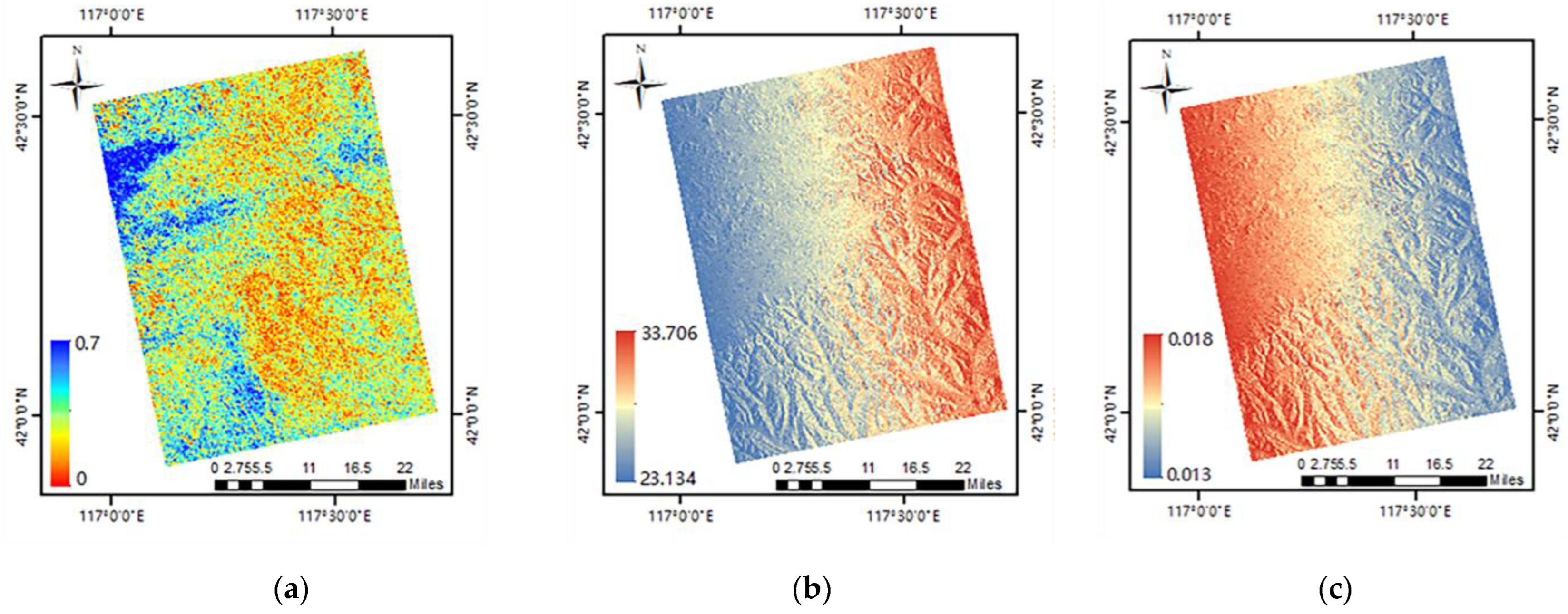
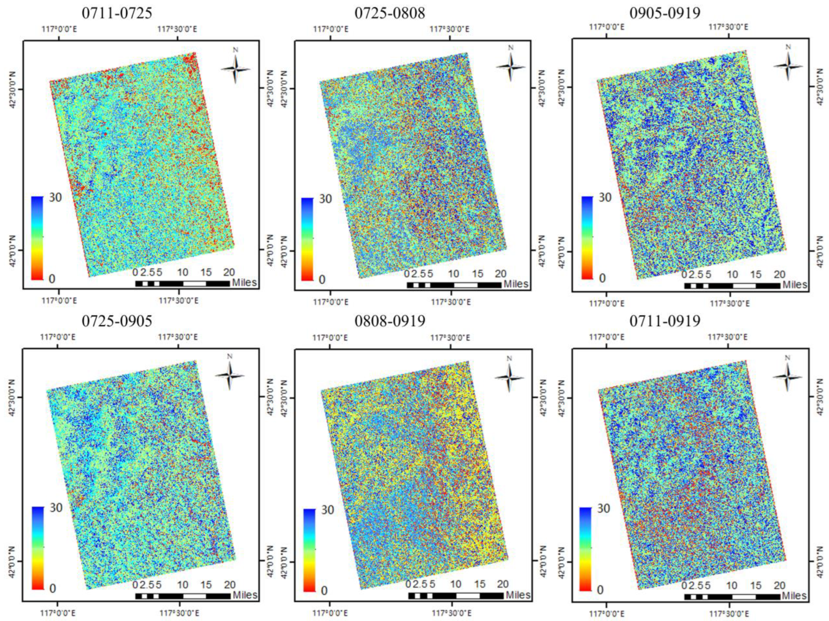
The ALOS-2 PALSAR data used in this study were based on L-band high-resolution synthetic aperture radar, which provides full-polarization 1.1-level SLC data and can obtain observation data independent of the climate conditions and time. Six interference pairs with different spatial and temporal baselines were established using five-view fully polarized data collected from July to September 2020 (

Table 3. Information on the ALOS-2 PALSAR data.

Master Image	Slave Image	Temporal Baseline (Days)	Vertical Wavenumber (rad/m)	Incidence Angle at the Scene Center (°)
0711	0725	14	0.013–0.018	27.8054
0725	0808	14	0.010–0.015	27.8029
0905	0919	14	0.015–0.020	27.7991
0725	0905	42	0.010–0.016	27.8029
0808	0919	42	0.016–0.020	27.8012
0711	0919	70	0.019–0.027	27.8054

), with a range resolution of 5.66 m and azimuth resolution of 2.86 m. GAMMA software was used to conduct geometric decorrelation preprocessing, such as radiometric calibration and filter denoising [30], and SRTM DEM data were used for the topographic correction and geocoding. Figure 3 shows the HV polarization coherence image (a), the local incident angle image (b) and the vertical wavenumber image (c) of the 0711-0725 interference pair obtained after the image preprocessing stage.

3. Theoretical Background of the RVoG Model

PolInSAR combines the characteristics of InSAR and PolSAR to provide sensitivity to the vertical distribution of different scattering mechanisms and to improve the accuracy of forest vertical structure inversion. For the two SAR images $s_1\left(\overrightarrow{w}\right)$ and $s_2\left(\overrightarrow{w}\right)$ acquired by interference with polarization $\overrightarrow{w}$, the complex interferometric coherence (including the amplitude and phase) can be expressed as:

$$\gamma =\frac{\langle s_1\left(\overrightarrow{w}\right)s_2^{*}\left(\overrightarrow{w}\right)\rangle }{\sqrt{\langle s_1\left(\overrightarrow{w}\right)s_1^{*}\left(\overrightarrow{w}\right)s_2\left(\overrightarrow{w}\right)s_2^{*}\left(\overrightarrow{w}\right)\rangle }}$$

(1)

where * is the conjugate of the SAR image, and 〈〉 is the expected value.

Coherence reflects the degree of consistency of the radar signals received by the primary and secondary antennas for the same target, which is determined by the temporal stability of the ground and vegetation scatterers in the resolution cell. It ranges from 0 to 1 and describes the degree of similarity between the homonymous regions of the two images. For completely coherent scatterers, $\gamma =1$. However, any variation between the two images results in decorrelation, and the observed interference coherence can be represented by the following contributions [31,32]:

$$\gamma ={\gamma }_{SNR}{\gamma }_{Temporal}{\gamma }_{Volume}$$

(2)

where ${\gamma }_{SNR}$ is decorrelation caused by system noise, ${\gamma }_{Temporal}$ is the reduction in interferometric coherence caused by changes in the scatterer during two repeated observations, and ${\gamma }_{Volume}$ is volume decorrelation, which usually occurs in the vegetation region and provides information on the vertical structure of the scatterer. It is usually expressed as the Fourier transform of the vertical structure profile function of the effective scatterer [33,34].

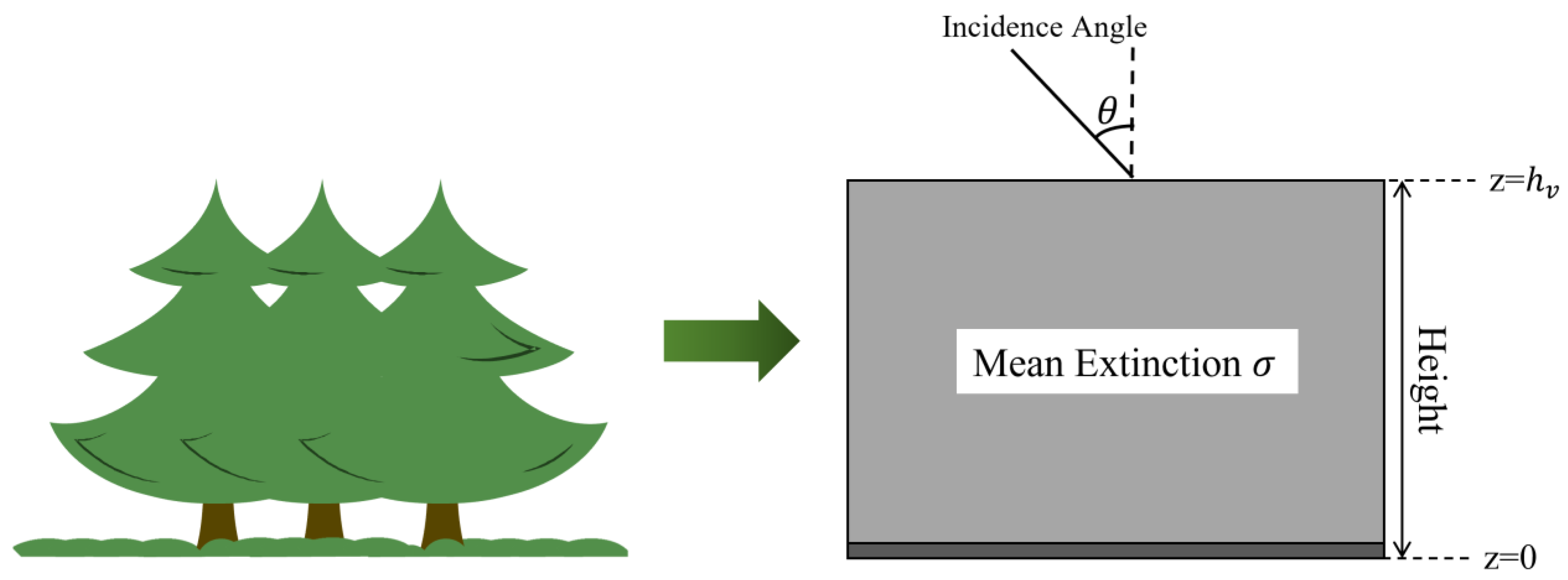
To estimate the forest height, the RVoG inversion model is frequently used, as it is fundamentally a physical model. The model relates the forest vertical structure parameters to complex interferometric coherence observations. In this model, the canopy is a homogeneous volume consisting of particles that are randomly oriented and have constant wave attenuation in a medium on the ground [9], as shown in Figure 4. The interference scattering process of the forest scene, which consists of a volume layer on the underlying surface, is described by the two-layer RVoG model. Volume decorrelation ${\gamma }_{Volume}$ is directly related to the vertical distribution of the scatterer through the (normalized) Fourier transform relation, which can be written as a function of the volume coherence ${\gamma }_V$, expressed as:

$${\gamma }_{Volume}=e^{j\phi }\frac{{\gamma }_V+m}{1+m}$$

(3)

$${\gamma }_V=\frac{{{\displaystyle \int }}_0^{h_v}{e}^{\frac{2\sigma }{\mathit{cos}\theta }z}{e}^{j{k}_{z}Z}dz}{{{\displaystyle \int }}_0^{h_v}{e}^{\frac{2\sigma }{\mathit{cos}\theta }z}dz}=\frac{e^{\frac{2\sigma }{\mathit{cos}\theta }{h}_v+j{k}_z{h}_v}-1}{\left(e^{\frac{2\sigma }{\mathit{cos}\theta }{h}_v}-1\right)}\frac{2\sigma }{2\sigma +j{k}_z\mathit{cos}\theta }$$

(4)

$$m=\frac{{\omega }^{*T}{T}_G\omega }{{\omega }^{*T}{T}_V\omega }$$

(5)

where $m$ represents the ground-to-volume scattering ratio, $\phi$ is the ground phase, and $\theta$ is the incident angle of the radar. ${\gamma }_V$ is pure volume scattering complex coherence, which is a function of the vegetation layer thickness $h_v$ and the mean extinction coefficient $\sigma$, $T_G$ and $T_V$ are the echo signal intensity of the ground and vegetation layers, respectively, and $\ast T$ represents the conjugate transpose.

$k_z$ is the vertical wavenumber, which is a function of the deviation of the incidence angle caused by the baseline. The $k_z$ value is higher near the small incident angle, and it decreases when it is far from the increasing incident angle [35], as follows:

$$k_z=m\frac{2\pi }{\lambda }\frac{B_{\perp }}{R\sin \left(\eta \right)}$$

(6)

where $m$ is an integer constant, which is equal to 2 in the case of monostatic acquisition and 1 in the case of a bistatic acquisition. $\lambda$ is the wavelength, $B_{\perp }$ is the vertical component of the spatial baseline, $R$ is the radar slope distance, and $\eta$ is the local incidence angle.

The three-stage inversion method is an improved forest height inversion technique based on the RVoG model. The complexity of the model is simplified by fixing the extinction coefficient value, which includes three main steps. Firstly, the complex coherence coefficients of the different polarization interference combinations are calculated, and then a line of coherence coefficients is obtained on the complex unit circle by fitting the real and imaginary parts of the coherence coefficients by the least squares so as to realize the least squares fitting of the multi-polarization interference coherence coefficients in the complex plane. After that, maximum vegetation deviation removal and ground phase estimation are performed, according to the principle of the maximum deviation of vegetation to determine which one of the two-phase intersections is a real phase, first the GVR corresponding to each polarization is estimated separately, then the corresponding minimum m value is determined, its phase distance from the two intersection points is calculate, and that which is furthest away from the intersection as the ground phase point $\phi$ is selected. Finally, the vegetation height and extinction coefficient are estimated using the iterative estimation of the mean squared deviation minimization principle. According to the minimum distance between the calculated volume coherence points and the observed coherence points, the LUT of the variation in the volume-only complex coherence ${\gamma }_V$ with the forest height and $\sigma$ is established. From the ground phase estimated in the second step, it is easy to determine the coherence point ${\gamma }_V$ that is farthest from it in the observed data. By comparing the estimated value of ${\gamma }_V$ with the lookup table, the estimated values of $\sigma$ and the forest height can be obtained [12,32].

4. Proposed Method of the Research

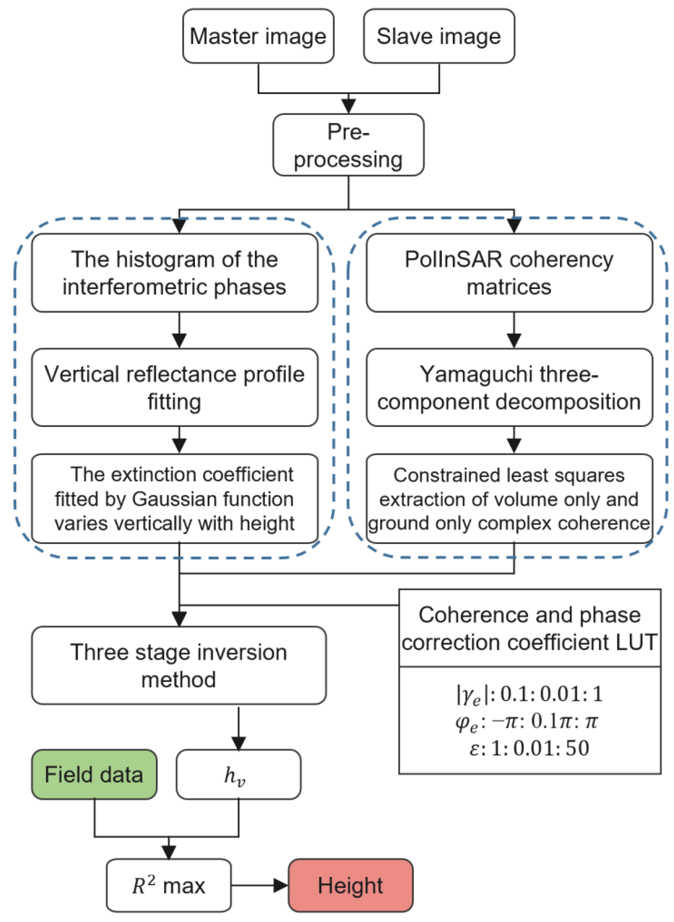
Figure 5 shows the flowchart of the proposed forest height inversion method.

4.1. Semi-Empirical Improved RVoG Inversion Model

In the microwave region, the dielectric properties of vegetation are significantly influenced by its water content and geometric characteristics (e.g., the stems, branches and leaves), as well as the movement of the scatterers (leaves and fine branches) between data acquisitions, resulting in differences in displacement due to vegetation movement. Depending on the frequency and polarization, these factors have different degrees of influence on scattering in temporal decorrelation [28]. Temporal decorrelation reduces the coherence and causes phase shifts in the interferometric data, which have a significant impact on the forest height inversion model. Moreover, its error sources have a complicated structure and are affected by a combination of factors that are difficult to quantify, rendering temporal decorrelation difficult to eliminate when preprocessing image data [36]. This has a greater impact on PolInSAR forest height inversion and, consequently, measures must be taken to reduce this interference.

In previous studies, the physical model construction method was used to decompose temporal decorrelation into dielectric constant, random motion and other components, which were then modeled together with volume decorrelation to extract the forest height [36]. Different images produce different degrees of temporal decorrelation effects with the same disturbance. PolInSAR data with smaller $k_z$ show more obvious responses to temporal decorrelation, and the inversion of the forest height is more sensitive to the coherence and phase changes of the interference data [19]. Therefore, when using interference images with small $k_z$ to retrieve the forest height, the inversion results may have large errors, even in the presence of a weak temporal decorrelation [20]. This situation is indicated by the fact that the complex coherence shown in the unit circle does not intersect the LUT when using the three-stage inversion method for height inversion [12]. In fact, the $k_z$ of repeat-pass spaceborne PolInSAR data tends to be low (already containing a large temporal decorrelation factor), leading to the low accuracy of the inversion results. Therefore, an effective correction of $k_z$ is required to ensure high accuracy in forest height extraction.

In this study, considering no deformation of the ground surface during the two imaging periods and overlooking atmospheric disturbances and noise interference, only the flat earth phase and topographic phase remain in the interferometric phase. $k_z$ is a factor that indicates the sensitivity of the interferometric phase to terrain (height) variation (Equation (6)). Thus, the linear relationship between the height and terrain phase can be connected by $k_z$ [19]. The interferometric phase variation is analyzed by combining the flat earth phase ${\phi }_{flat}$ and topographic phase ${\phi }_{topo}$, as follows:

$$\Delta \phi ={\phi }_{topo}-{\phi }_{flat}=-k_z·h-{\phi }_t$$

(7)

where the first term on the right side of the equation is the terrain phase caused by terrain height, and ${\phi }_t$ is the flatland phase caused by no elevation change. A linear relationship between height and terrain phase connected by $k_z$ is established when the flatland phase is removed.

When measuring the forest height using PolInSAR, there are major differences in the interferometric measurements of the terrain height. Therefore, when measuring the forest height, the interferometric phase of the upper point of the canopy and the bottom mat point are must be incorporated into the calculation. However, there are two kinds of phase contributions. One is the shift of the phase center caused by the penetration of low-frequency SAR into the forest canopy, and the other major phase contribution is the phase shift caused by the random motion of the canopy during imaging of the primary secondary image [37]. Both contributions play interfering roles in the measurements and must be removed during the inversion. When the effects of the above two effects are considered, the phase changes, as follows:

$$\Delta \phi ={\phi }_{topo}-{\phi }_{flat}=-k_z·\left(h+\Delta h\right)-{\phi }_t$$

(8)

where $\Delta h$ is the height deviation resulting from the combined effect of the two effects.

The height offset can be thought of as a linear function of canopy height when only the offset from the random motion of the canopy is considered as follows:

$$\Delta h=\frac{H_r}{h_r}h={\epsilon }_{0}h$$

(9)

where $H_r$ represents the standard deviation of the motion at a certain reference height $h_r$ and ${\epsilon }_0$ indicates the change in this offset relative to the height.

The phase deviation due to low-frequency SAR penetration causes the observed phase between the top of the canopy and half of the height [38], therefore, considering the canopy phase shift due to random motion and the phase center deviation due to low-frequency SAR penetration, the height deviation obtained through the coupling of these two factors can be simplified to a linear function with the variation vertical target height.

$$\Delta h={\epsilon }_{0}h-d$$

(10)

where $d$ is the distance between the scattering center and the underlying surface after the canopy phase shift, $h/2\le d\le h$ [38].

By introducing the height error into the canopy phase after removing the flat earth phase, the relationship between the observed canopy phase ${\phi }_v$ and the true canopy height $h$ can be obtained as follows [37]:

$${\phi }_v=k_z\left(\left(1+{\epsilon }_0\right)h-d\right)=\epsilon k_{z}h-k_{z}d=\epsilon k_{z}h+{\phi }_e$$

(11)

where $\epsilon$ is the correction term of temporal decorrelation caused by random motion, ${\phi }_e$ is the correction phase of the phase center shift and $\epsilon \ge 1$, $-\pi \le {\phi }_e\le \pi$.

To solve the problem of temporal decorrelation in the inversion of PolInSAR data, a new inversion method was proposed that realizes the inversion of the forest height through empirical iteration. The semi-empirical improved RVoG inversion model integrates the error factors encountered in the inversion process to provide an overall correction of the offset phase caused by random motion and microwave penetration factors and the coherence errors caused by dielectric constants [37]. Three correction terms, namely, $\epsilon$, ${\phi }_e$ and ${\gamma }_e$, are introduced based on the RVoG model. ${\gamma }_e$ is the correction of temporal decorrelation according to the overall coherence, and the correction of the phase influence of temporal decorrelation on $k_z$ is realized using $\epsilon$ and ${\phi }_e$. The correction term in the phase and the complex coherence correction term are introduced into the iteration process to ensure that the full error source is considered in the model:

$$\begin{gathered} {\gamma }_V=\left|{\gamma }_e\right|\frac{2\sigma }{\mathit{cos}\theta \left(e^{\frac{2\sigma }{\mathit{cos}\theta }{h}_v}-1\right)}{{\displaystyle \int }}_0^{h_v}{e}^{\frac{2\sigma }{\mathit{cos}\theta }z}{e}^{j(\epsilon k_{z}Z+{\phi }_e)}dz \\ {\gamma }_V={\gamma }_e\frac{2\sigma }{\mathit{cos}\theta \left(e^{\frac{2\sigma }{\mathit{cos}\theta }{h}_v}-1\right)}{{\displaystyle \int }}_0^{h_v}{e}^{\frac{2\sigma }{\mathit{cos}\theta }z}{e}^{j(\epsilon ·k_z)Z}dz \\ {\gamma }_e=\left|{\gamma }_e\right|·e^{j{\phi }_e} \end{gathered}$$

(12)

4.2. Extinction Coefficient

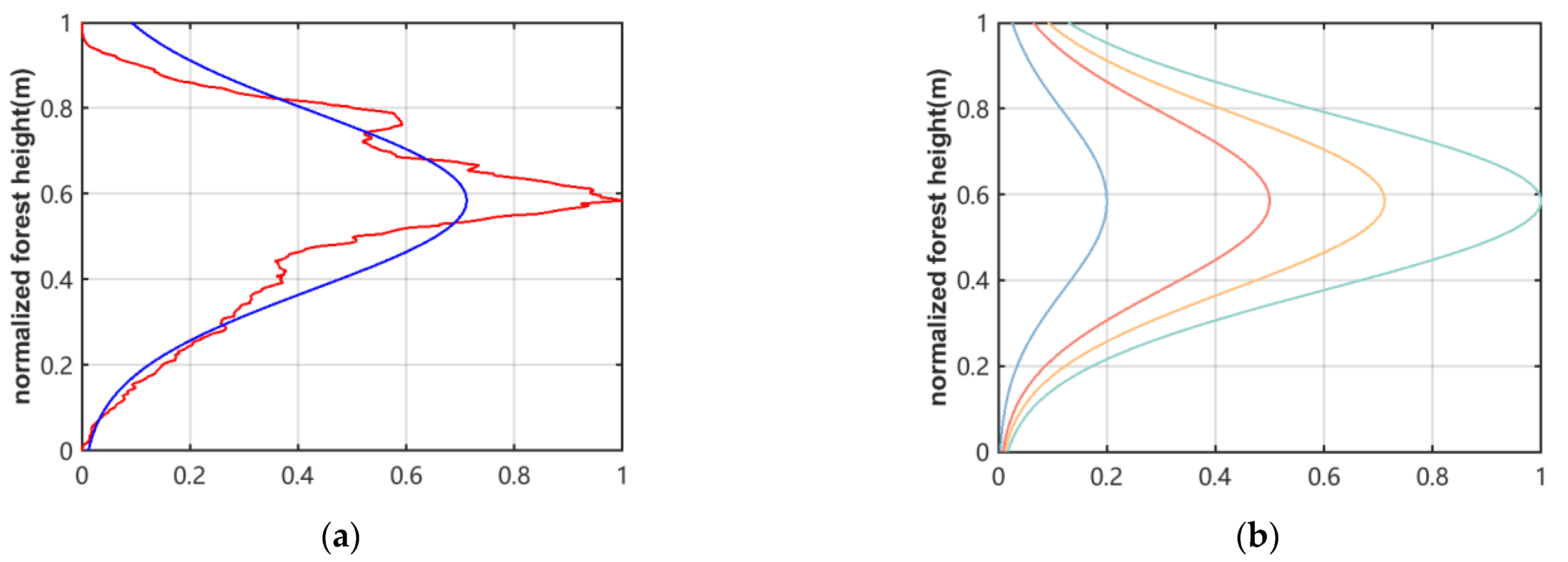
The extinction coefficient represents the attenuation rate of microwaves in the forest volume, which is a function of the density of scatterers in the forest and its dielectric constant, reflecting the environmental conditions of the forest [9,39]. The existing RVoG model assumes that the extinction coefficient σ is a constant value of a uniform vegetation volume, which cannot describe the forest heterogeneity in the vertical direction. However, forests have different vertical structures from the canopy to the ground, including the leaf, branch and trunk layers. The vertical structure of the forest has a significant effect on the extinction coefficient and influences the inversion of the forest parameters. In fact, in the case of heterogeneous forests, the material density at the top of the canopy is lower than that at the bottom of the forest, and the inhomogeneous distribution of scatterers in the volume causes the value of the extinction coefficient σ to vary with height. Therefore, a more suitable model for height inversion must investigate how one can accurately describe the vertical forest structure. In recent years, polarization coherence tomography (PCT) has been rapidly developed and used to estimate the vertical backscattering profiles of forests in the L-band [40], but the theoretical research on the technique is complex, and its practical application is challenging. Meanwhile, the Lidar waveform has been widely used to determine the vertical reflectance profile structure [41], but the acquisition of Lidar data is expensive, and the data cannot cover a large area. In this study, we use a converted InSAR phase center height histogram to provide an approximation of the vertical reflectance profile [42,43] and fit the extinction coefficient function with the height according to the shape of the vertical reflectivity profile, allowing us to avoid the problems of expensive LiDAR data and the complex PCT research theory. The interference phase histogram is used to provide an approximation of the vertical reflectance profile, and the vertical extinction coefficient curve is expressed as a function of height using a Gaussian function [21]:

$$\sigma =a·exp\left[-{\left(\frac{z-u}{v}\right)}^2\right] 0\le z\le h_v, a>0$$

(13)

where $h_v$ is the thickness of the vegetation layer, $a$ is the influence factor of $\sigma$, $u$ is the position of maximum extinction in the forest canopy, $v$ is the standard deviation represented by the canopy shape and $u$ and $v$ reflect the vertical heterogeneity of the forest.

The $v$ value increases with the canopy height and vice versa. When the value of $v$ approaches infinity or 0, the extinction coefficient approaches $a$ and 0, respectively. Under these two extreme conditions, the volume coherence can be simplified to the RVoG model and SINC model after introducing the above extinction coefficient function.

4.3. PolInSAR Decomposition Technique

The GVR is the ratio of the scattering energy generated by the electromagnetic wave on the ground and the vegetation canopy, which determines the relative scattering contribution of the ground and volume layer and depends on the polarization mode. Different GVRs correspond to different physical properties of the vertical structure and polarization characteristics of ground scattering and volume scattering. Usually, the GVR is customized using the RVoG model, but the RVoG model cannot distinguish between two ground responses, specifically direct scattering with the trunk and the interaction with double-bounce scattering, while the PolInSAR-based polarization decomposition algorithm includes all the beneficial characteristics of radar data decomposition, resolving the issues with the RVoG model mentioned above [7]. This study combines the potential of polarization decomposition to obtain different scattering mechanisms with the ability of interference estimation to determine the vertical positions of different scatters in order to separate the ground and volume coherence matrices. The polarization decomposition concept of Yamaguchi three-component decomposition is applied to PolInSAR data.

Instead of the most widely known form of decomposition, namely Freeman three-decomposition, Yamaguchi three-component decomposition was selected to improve the GVR because it improves on the Freeman decomposition method by manually compensating for the polarization azimuth angle and modifying the volume scattering probability density function to reduce errors when distinguishing between volume scattering and double-bounce scattering, which are more suitable for the mapping of forest parameters due to the distinct physical properties related to scattering [44,45]. The covariance matrix obtained from PolInSAR observation data is decomposed into three scattering mechanism matrices, as proposed by Yamaguchi for PolSAR data, so as to more accurately distinguish the scattering responses from the ground and the overlying vegetation [26]. In this study, we considered the influence of a larger GVR on the accuracy of forest height inversion, which is caused by the fact that electromagnetic waves in sparsely vegetated areas can easily penetrate the vegetation layer and reach the ground, thus resulting in a stronger ground echo signal, and the fact that there is more double-bounce scattering caused by tree growth and trunk interaction, which is considered as ground scattering [46]. With this in mind, we established a new GVR parameter that considers volume scattering and even scattering as volume layer scattering and odd scattering as ground layer scattering so as to avoid the limitations of GVR generation to a certain extent, as follows:

$$m=\frac{{\omega }^{*T}{T}_s\omega }{{\omega }^{*T}(T_{Vol}+T_d)\omega }=\frac{{\omega }^{*T}{T}_G\omega }{{\omega }^{*T}{T}_V\omega }$$

(14)

where $T_s$, $T_d$ and $T_{Vol}$ represent the contributions of surface, double-bounce and volume scattering components, respectively. $T_d$ and $T_{Vol}$ are considered as the volume layer scattering $T_V$ and $T_s$ as the ground layer scattering $T_G$.

The ground and volume scattering contribution coherence matrices are reconstructed using the RVoG model and PolInSAR decomposition technique. Firstly, polarization interference information is extracted from the preprocessed PolInSAR data. Each pair of polarization interference data contains the original complex data at full polarization. The scattering matrix defined by the Pauli basis can be equivalently described by the scattering vector, provided that the scatterer satisfies the reciprocity condition:

$$\begin{gathered} K_1=\frac{1}{\sqrt{2}}{\left[S_{1HH}+S_{1VV} S_{1HH}-S_{1VV} 2S_{1HV}\right]}^T \\ {K}_2=\frac{1}{\sqrt{2}}{\left[S_{2HH}+S_{2VV} S_{2HH}-S_{2VV} 2S_{2HV}\right]}^T \end{gathered}$$

(15)

where $S$ represents the scattering matrix elements obtained at different polarizations, and $T$ represents the transpose of the matrix.

The PolInSAR coherence matrices, namely the polarization ($T_{11}$ and $T_{22}$) and cross-correlation (${\Omega }_{12}$) coherence matrix, are extracted as follows [26,47]:

$$\left[T_6\right]=\langle \left[\begin{array}{c}{K}_1\\ K_2\end{array}\right] \left[K_1{}^{*T} K_2{}^{*T}\right]\rangle =\left[\begin{array}{c}\langle K_1{K}_1{}^{*T}\rangle \langle K_1 K_2{}^{*T}\rangle \\ \langle K_2{K}_1{}^{*T}\rangle \langle K_2 K_2{}^{*T}\rangle \end{array}\right]=\left[\begin{array}{c}{T}_{11} {\Omega }_{12}\\ {\Omega }_{21} T_{22}\end{array}\right]$$

(16)

where $\ast T$ represents the conjugate transpose operator. ${\Omega }_{12}$ is a 3 ∗ 3 non-Hermitian complex matrix that contains polarization and interference information. $T_{11}$ and $T_{22}$ are Hermitian positive semidefinite matrices, which contain the polarization features of each image.

The maximum likelihood estimate of the polarization coherence matrix $T$ is obtained using the polarization stationary assumption [48,49]:

$$T=\frac{1}{2}\left(T_{11}+T_{22}\right)$$

(17)

The coherence matrix based on the model assumption can be decomposed into a ground layer and a volume layer:

$$T=f_G{T}_G+f_V{T}_V$$

(18)

where $T_G$ and $T_V$ are the ground matrix and volume coherence matrix, respectively, and $f_G$ and $f_V$ are the contributing factors related to the ground layer and volume layer, respectively.

The interference behavior of the main scattering contribution of a layer of random volume vegetation on the ground can be modeled by a linear combination of polarization interference correlation matrices as follows:

$${\Omega }_{12}=f_G{\Omega }_G+f_V{\Omega }_V$$

(19)

Based on the assumption that the polarization of all the decorrelation sources is independent, it can be expressed as [50]:

$${\Omega }_{12}=f_G{T}_G{\gamma }_G+f_V{T}_V{\gamma }_V$$

(20)

where ${\gamma }_G$ and ${\gamma }_V$ are ground-only and volume-only complex coherence, respectively.

Thus, a system of linear equations is obtained in which the unknown parameters, namely, ${\gamma }_G$ and ${\gamma }_V$, can easily be estimated. It should be noted that there must be pure ground coherence and pure volume coherence on the coherence lines of the unit circle. Therefore, Equation (20) is transformed into a constrained linear least squares problem, where the phases of ${\gamma }_V$ and ${\gamma }_G$ are taken as the observed volume phase and ground phase, respectively, using the least squares method.

5. Results

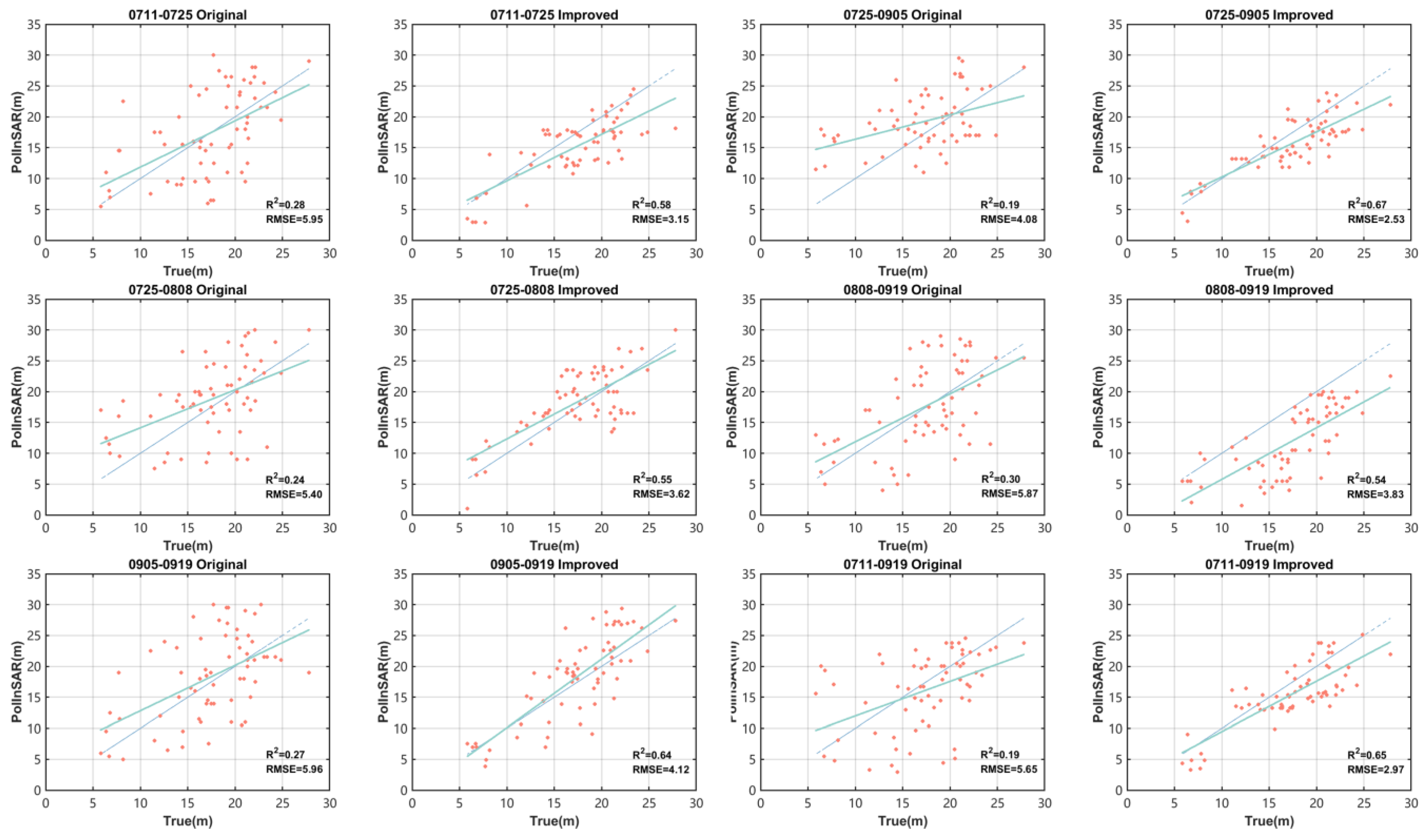
The improved forest height inversion model was created by introducing the variable extinction coefficient and the improved GVR findings obtained using the above method into the semi-empirical improved RVoG model. Figure 6 shows the inversion height results obtained using the original model and the improved model, with some improvement in the overall accuracy. However overall underestimation is still apparent.

Table 4. Results regarding the parameter iteration and precision of inversion. Both RMSE and R² have two values, which are the results of the original model and the improved model, respectively.

Datasets	Parameters		Accuracy		Result
	$\mathit{\epsilon }$	${\mathit{\gamma }}_{\mathit{e}}$	RMSE	${\mathit{R}}^2$	$\mathbf{Average} \mathit{\epsilon }{\mathit{k}}_{\mathit{z}}$
0711-0725	29.15	$0.60\times e^{-i·\pi }$	5.85/3.15	0.28/0.58	0.3148
0725-0808	38.89	$0.17\times e^{i·0.6\pi }$	5.40/3.62	0.24/0.55	0.3422
0905-0919	40.02	$0.60\times e^{-i·0.5\pi }$	5.96/4.12	0.27/0.64	0.5203
0725-0905	39.57	$0.24\times e^{-i·0.2\pi }$	4.08/2.53	0.19/0.67	0.3680
0808-0919	29.88	$0.10\times e^{i·0.1\pi }$	5.87/3.83	0.30/0.54	0.3944
0711-0919	37.09	$0.19\times e^{i·0.4\pi }$	5.65/2.97	0.19/0.65	0.5897

shows the inverse accuracy of the model. It can be seen that the $R^2$ values of the improved model were all above 0.5, which indicates a certain degree of improvement in the accuracy compared with the original model and better fitting outcomes. The iteration parameter $\epsilon$ ranged from 20 to 50, demonstrating that the phase inaccuracy of the repeat-pass spaceborne PolInSAR data was significantly impacted by the random motion of the canopy. The decorrelation correction term ${\gamma }_e$ increased with the increase in the temporal baseline for the first five images, which indicates that the improved model has a good correction effect on the temporal decorrelation interference. However, in the 0711-0919 interferometric image, the effect of the excessive temporal baseline on the image was too large to be fully explained by the temporal decorrelation term alone. This indicates that when the temporal baseline reaches a certain level, it is necessary to consider the magnitude of both the iteration parameter $\epsilon$ and the decorrelation correction term ${\gamma }_e$ in order to analyze the error caused by temporal decorrelation. At the same temporal baseline, the final $k_z$ value increased with the decreasing incident angle of the image center, and the magnitude of $\epsilon$ was related to the initial $k_z$ value. With the same image center incidence angle, the larger the temporal baseline was, the larger the initial $k_z$, $\epsilon$ and corrected $k_z$ value were, and the smaller the decorrelation correction term ${\gamma }_e$ was. That is, the magnitude of $\epsilon$ increased with the increase in the temporal baseline of the collective data, while ${\gamma }_e$ decreased with the increase in the temporal baseline. Although the $k_z$ compensation algorithm can invert the forest height rather accurately, it still has a small margin of error. Compared with the temporal baseline, $k_z$ has a more evident impact on the inversion results. The inversion results are accurate for large $k_z$ in general. After the linear cancellation of the influence on decorrelation, the robustness and accuracy of inversion were significantly improved, thus possibly satisfying the requirements for the remote sensing inversion of the forest height.

Figure 7 shows the forest height map obtained through the inversion of each pair of interference images. The 0711-0919 and 0905-0919 interference pairs had a better overall inversion effect, and the two images obtained larger vertical wavenumbers after correction, ensuring the better removal of the interference of temporal decorrelation. The other four images were affected by $k_z$, and with the decrease in $k_z$, the inversion results for the right side of the image were significantly underestimated. After correction, the $k_z$ values of the four images were relatively small, preventing the complete removal of the phase effect caused by temporal decorrelation on the vertical wavenumber. Moreover, the image of 0808-0919 was seriously underestimated, and the decorrelation correction term ${\gamma }_e$ was the smallest and was still clearly affected by the temporal decorrelation, only partially correcting the effect of temporal decorrelation on the sample data.

6. Discussion

6.1. Extinction Coefficient

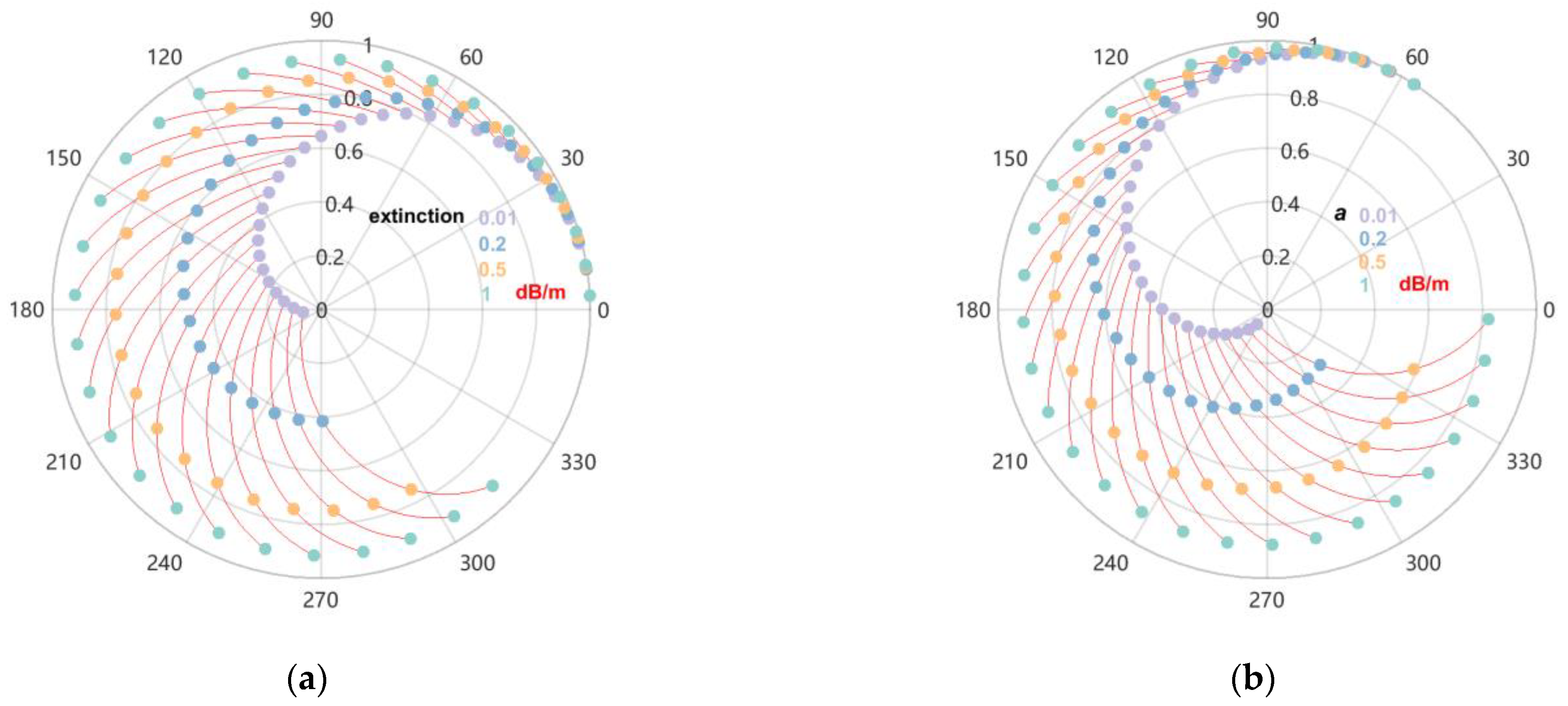
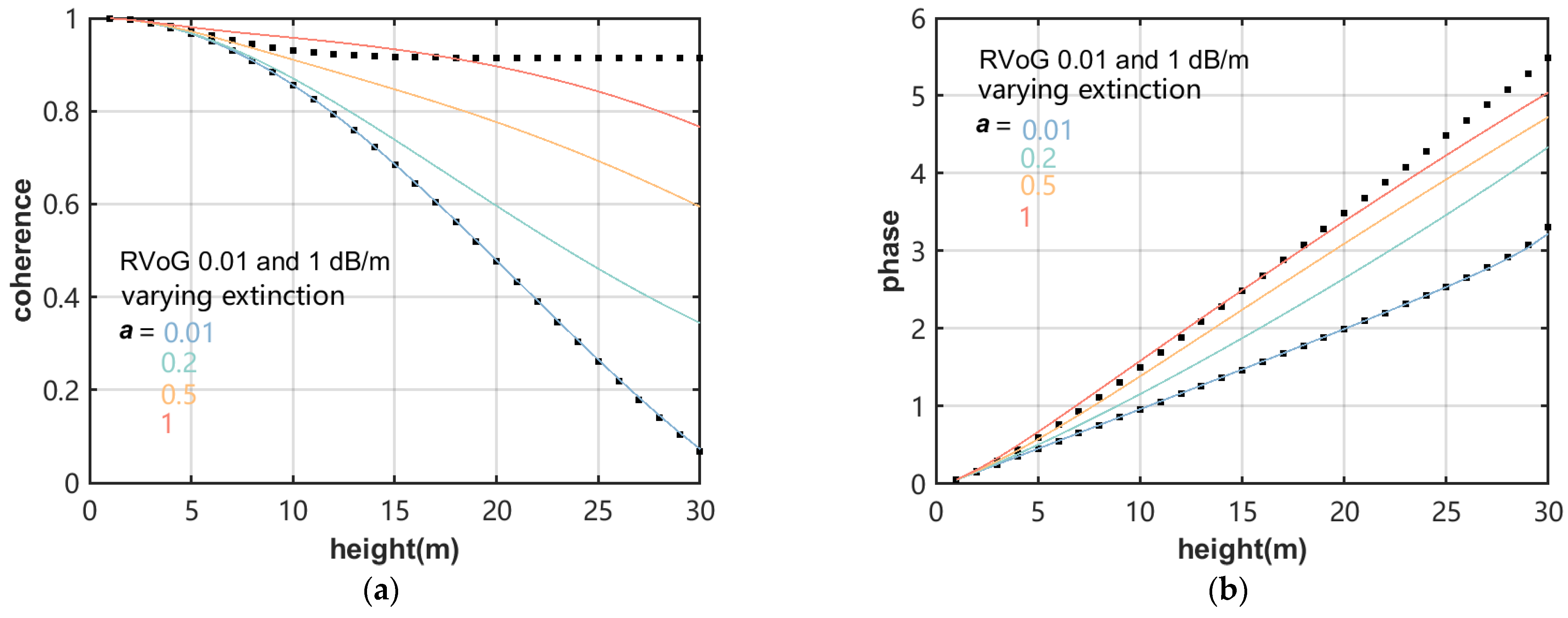
The constant extinction coefficient RVoG model and the variable extinction coefficient semi-empirical improved RVoG model were used to build the LUTs, which are shown in Figure 8a,b, respectively. We observed that when the extinction coefficient is zero, the impact of volume decorrelation is the most significant, because the scatterers distributed throughout the forest height interval contribute the same intensity and the radial position of the interference position is closest to the triangle of the circle center. When the extinction coefficient is large or the ground scattering is strong, the volume complex coherence amplitude easily becomes saturated, but the phase is not saturated (green curve). With the highest extinction coefficient is the highest, the smallest volume decorrelation, and largest phase center height. The volume coherence of the extinction coefficient in the range of 0–1 dB/m (red curve) varies with $h_v$. When the forest height is the same, the scattering amplitude of volume complex coherence is larger due to the strong surface scattering or vegetation attenuation, and volume decorrelation causes the complex coherence to decrease with the increasing vegetation height. Therefore, the increase in the extinction coefficient affects the volume decorrelation and phase center. The interference coherence of the varying extinction volume at low heights is close to the constant zero extinction random volume, the total change in the volume of the average extinction coefficient is lower, and the difference between the various extinction change rates becomes more significant with the increasing forest height. Furthermore, compared with the complex coherence obtained by constant extinction coefficient, it was found that the complex coherence obtained by varying the extinction coefficient simultaneously affects the phase center and coherence by introducing the temporal decorrelation correction factor. Figure 9 shows the coherence and phase of the extinction volume variation with height, where the linear variation in the coherence and phase at a constant extinction (0.01 and 1 dB/m) yield random volume boundaries. Comparing the coherence and phase variations obtained by the fixed extinction coefficient and extinction coefficient influence factor, it was found that the lowest and highest extinction coefficient influence factors are close to the properties of the constant extinction random volume model, and high extinction results in less volume decorrelation and a higher phase center height than low extinction.

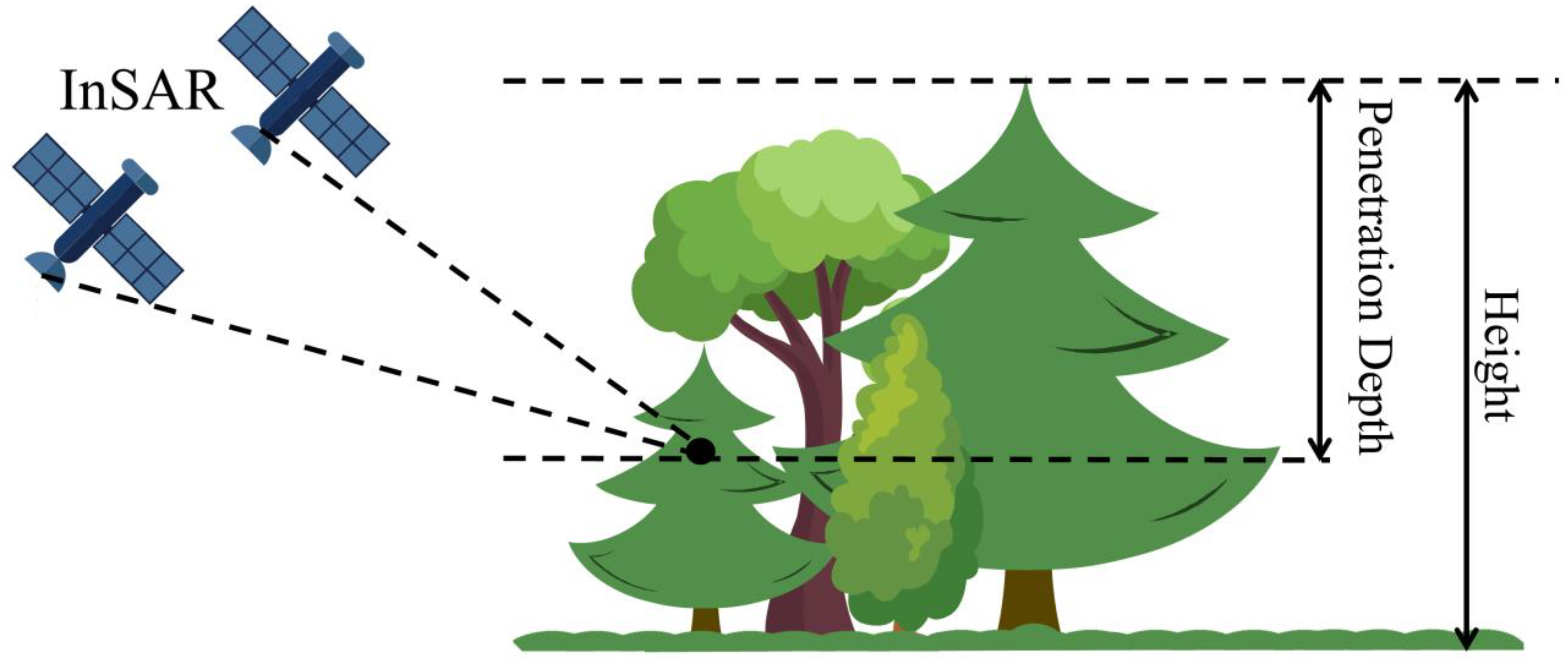
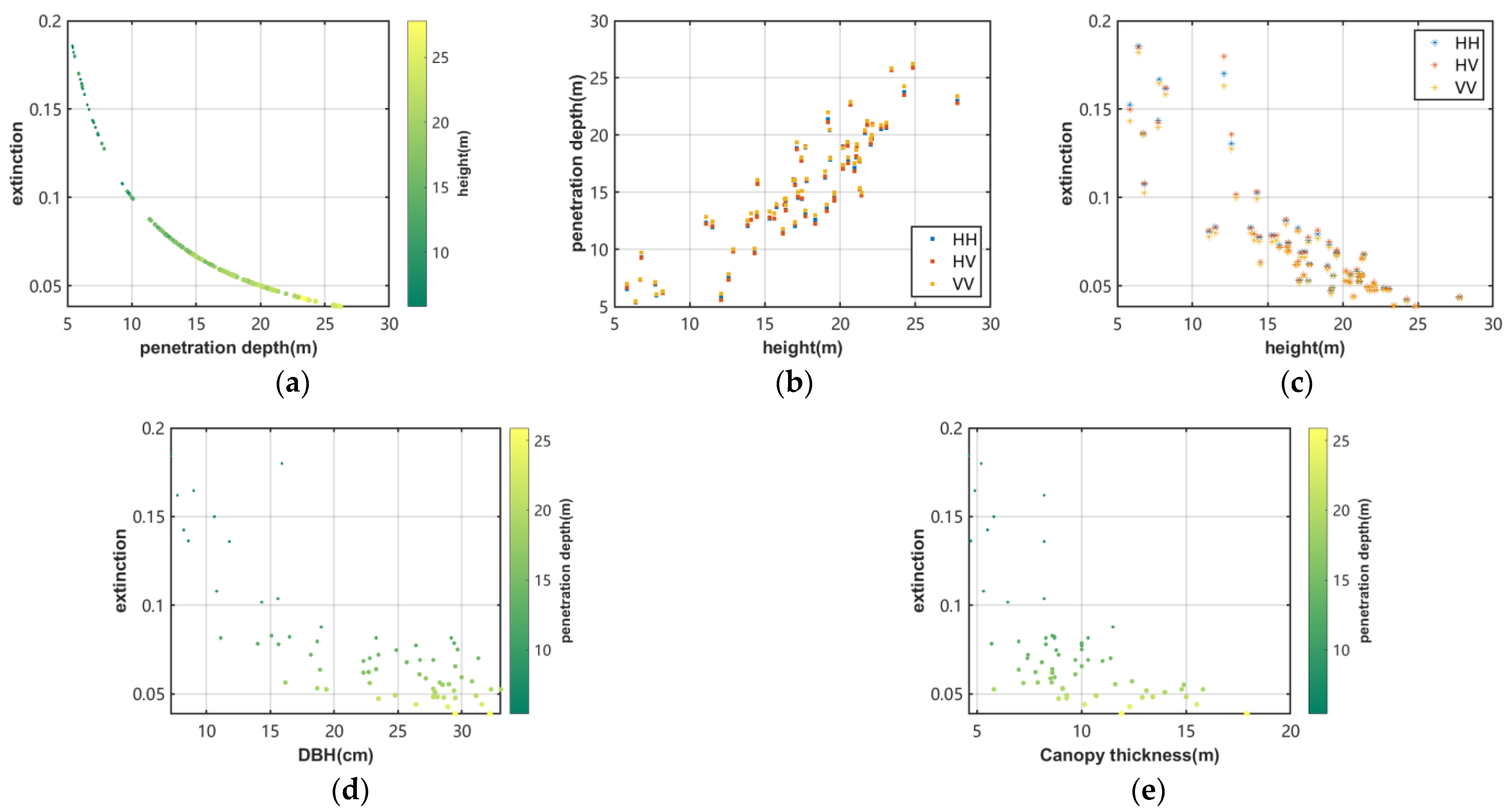
Since L-band data, which have an excellent electromagnetic wave penetration ability and a low phase center, were used in this study, the relationship between the vertical structure and electromagnetic wave attenuation was analyzed using the penetration depth. Penetration depth refers to the distance from the top of the canopy to the scattering phase center, and the interaction of the radar wavelength with canopy density and thickness determines the degree of canopy penetration and the degree of microwave attenuation (namely, the magnitude of the extinction coefficient) [51] (Figure 10). The scattering mechanism is directly related to the medium structure and its internal geometry. The vertical ordering of the polarization phase centers changes with the increasing forest height, indicating that the change in the forest structure during tree growth can affect the vertical distribution of the scattering mechanism [43]. Figure 11b shows that the penetration depth of HV polarization remained low in the canopy throughout the entire range of forest heights, whereas the vertical position of the phase center of HH polarization and VV polarization changed with the forest height and were more strongly affected by the stand density, indicating that the effect of the stand density on the interference signal received by the cross-polar channel was less significant [43,52]. The position of the phase center height derived from the interferometric data depends on the relative contributions of various scattering components, which, in turn, depend on the extinction coefficient. Changes in the forest stand density and canopy thickness can affect the extinction effect, and the forest stand density distribution is an important factor affecting the extinction coefficient. A rapid increase in the forest stand density can result in the formation of a closed canopy, leading to the further attenuation and depolarization of leaves and small branches through volume scattering, which manifests as an increase in the extinction coefficient [53]. The increase in the extinction effect reduces the interactions between radar signals and trees, and reduces the penetration of electromagnetic waves into the canopy, thus limiting the ability of microwaves to penetrate the vegetation canopy and causing the polarization scattering phase center to be close to the top of the canopy, which is conducive to the determination of forest height [54]. In this study, both the DBH and canopy thickness decreased with the increasing extinction coefficient (Figure 11d,e). Combined with changes in the relationship between the sample plots, it was found (Figure 2) that both the DBH and canopy thickness decreased exponentially with the increasing forest stand density. Therefore, the extinction coefficient increased with the increase in forest stand density, which led to the decrease in the penetration depth. This conclusion is the same as that obtained in the existing research [52]. Clearly, the extinction coefficient is closely connected to the forest height and canopy thickness [55,56].

All of the sample plots were pure coniferous forests with an equal distribution of trees and slight variation in the canopy height due to forests’ artificial nature. Therefore, in this study, we assumed that the normalized vertical structures of the trees in the forest were similar in a certain spatial domain and the SRTM DEM data was used to determine the transformed phase histogram to represent the vertical profiles of the trees in the region. The InSAR interferometric phase histogram was used to provide an approximation of the vertical reflectance profile, and the Gaussian function was used for the profile fitting so as to represent the vertical structural change in the extinction coefficient with height (Figure 12). The existing studies generally agree that HV polarization is more sensitive to the vegetation structure [57]. Thus, only the HV polarization of each interference pair was used to fit the vertical reflectance profile. Since there are no LiDAR data on the study area, the validation of the profile structure is not possible, but the structure of the obtained vertical reflectance profile structure conforms to the general scatterer distribution law [58]. The fitting result of the Gaussian function was good and represents the scatterer distribution well with respect to the extinction coefficient, which varies with height.

6.2. GVR

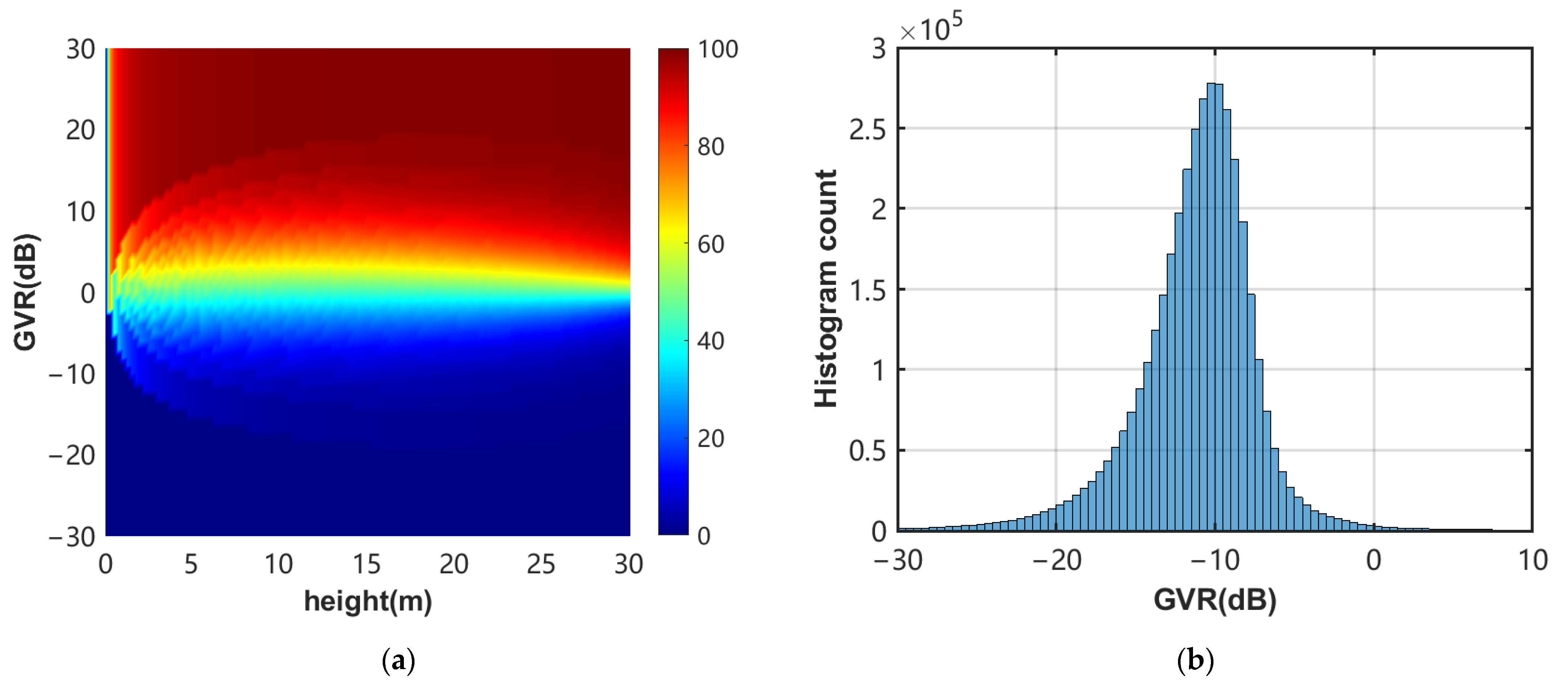
Zero GVR assumes ambiguity space in the calculation of volume-only coherence, especially in the case of sparse forest areas, since the contributions of volume and ground scattering are mixed in all polarization channels. Through the use of simulation experiments, the RVoG model was used to illustrate the degree sensitivity of the forest height to the GVR. In order to quantitatively analyze the forest height bias, the assumption of zero GVR was made for the forest height in the range of 0–30 m based on a GVR range from −30 dB to 30 dB. The simulation results show (Figure 13a) that when the GVR is less than −10 dB, the forest height is highly underestimated by 10%. The bias increases significantly as the GVR increases. The error is approximately 50% when the GVR approaches 0 dB, and the inversion of the forest height practically fails when the GVR exceeds 0 dB. Therefore, to ensure a certain level of accuracy in the estimation, the GVR should be lower than −10 dB. The improved GVR adopts the double-bounce and volume scatter as the scattering contribution of the volume layer, which enables one to avoid the error caused by the overestimation of the GVR in sparse vegetation areas. In general, the improved method can reduce the magnitude of the GVR, but it is still difficult to ensure that every GVR is below −10 dB (Figure 13b).

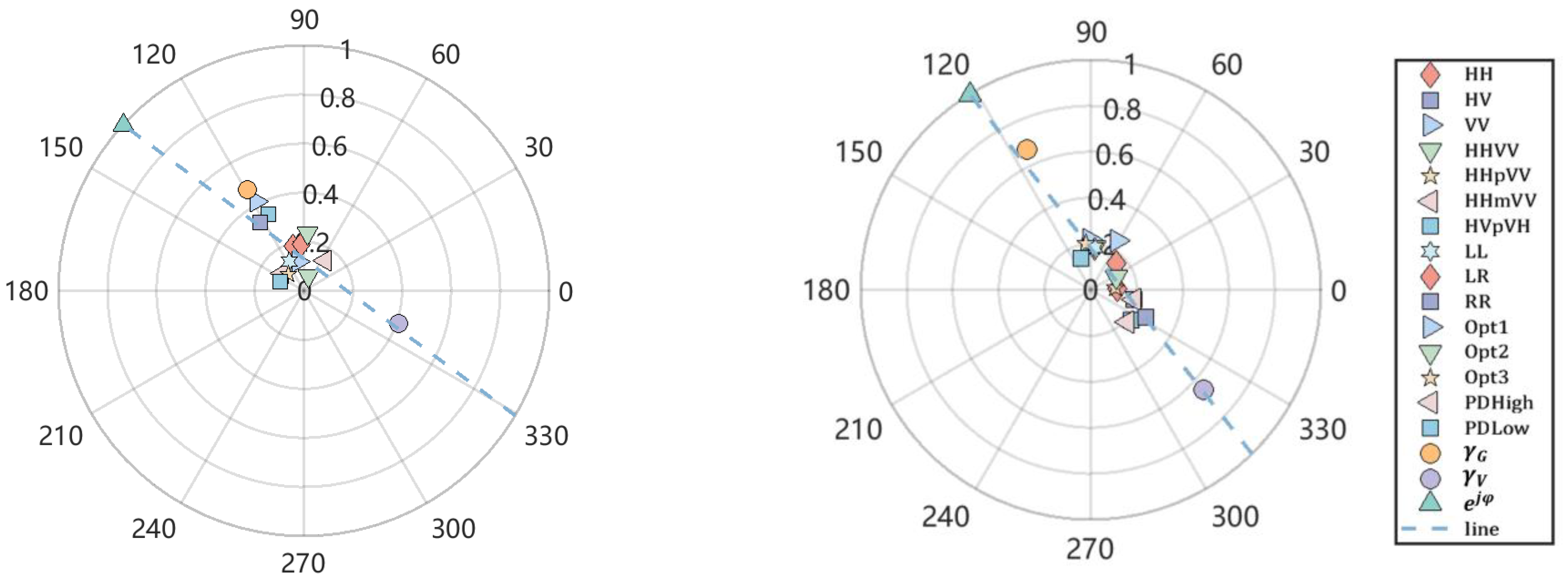
In order to analyze the relationship between the GVR and forest stand densities, the sample plots with the highest and lowest stand densities were selected in order to analyze the complex coherence (Figure 14). Fifteen complex coherence values that are common and easy to extract were used in this study to compare with the complex coherence values obtained in this paper, including three basic polarization types (HH, HV, VV), four linear combinations of different polarizations (HHVV, HH + VV, HH − VV, HV + VH), three circular polarizations (LL, LR, RR), three Opt coherence optimizations (Opt1, Opt2, Opt3), and two PD coherence optimizations (PD High, PD Low). It can be seen from Figure 14, the low-density complex coherences all converged together, while the high-density ones were relatively scattered. Because the electromagnetic wave easily penetrates the vegetation layer in low-density forest stands, the scattering phase of the high volume is close to that of the surface. However, the electromagnetic wave in high-density forest stands cannot easily penetrate the vegetation layer, and the scattering phase center of the high volume is far from the surface scattering phase. In the complex plane, the coherent points are scattered on both sides of the coherence line, which is beneficial for the fitting of the coherence line and the estimation of the ground phase. Moreover, there is more ground scattering, because the attenuation of the electromagnetic wave decreases in sparse forest when penetrating the vegetation layer. It can be observed that the ground-only and volume-only complex coherences obtained after the modification improve the estimation of the ground and volume phases to a considerable extent.

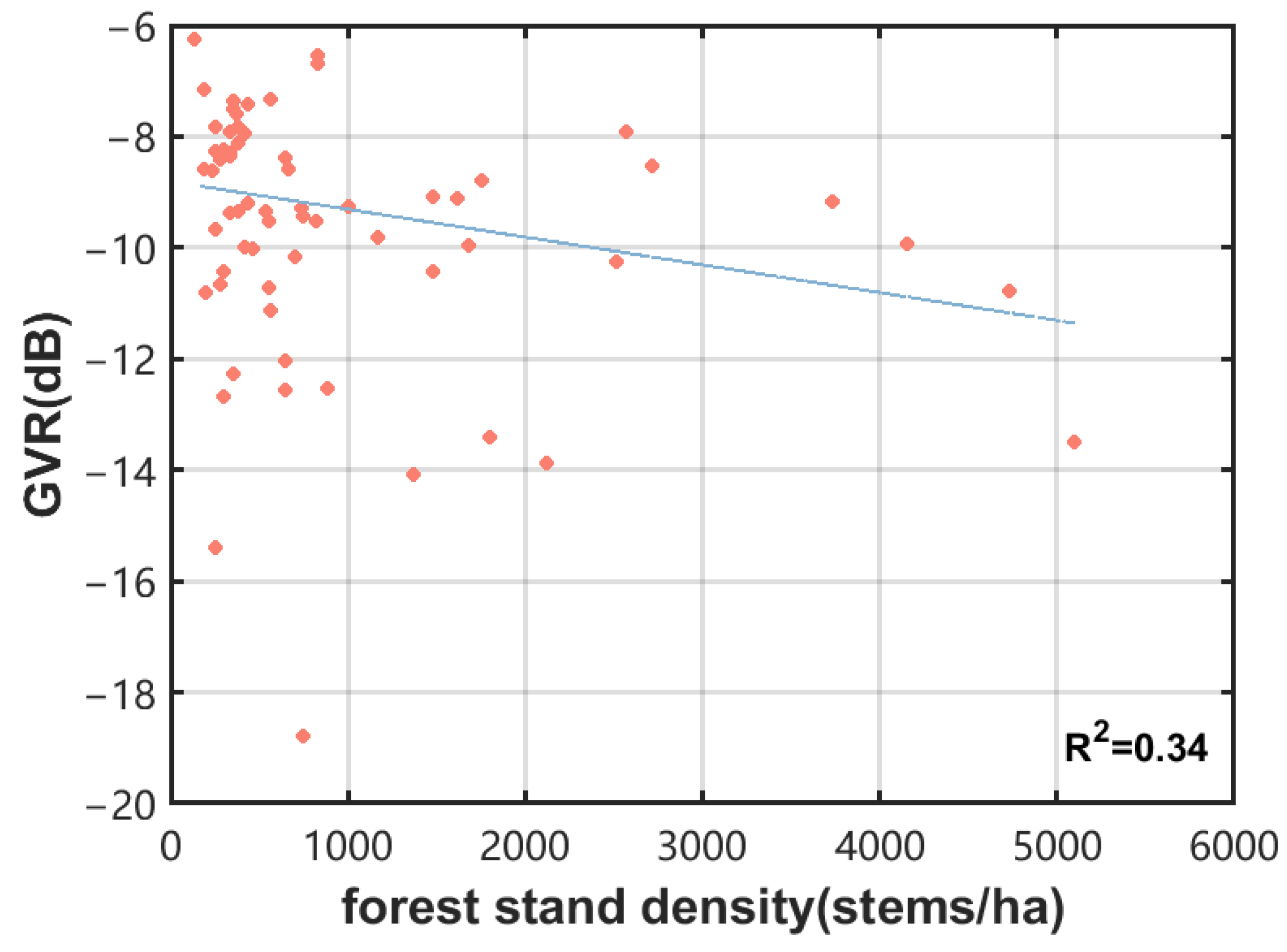
Because the L-band has penetrating properties, the volume and double-bounce scattering increase significantly with the increasing forest stand density and the growth of trees, and the GVR decreases, which is conducive to height inversion. For dense canopies, only the upper canopy returns to backscatter, which greatly increases scattering on the canopy surface, rather than volume scattering. Compared to dense forests, in sparse forests, electromagnetic wave attenuation decreases when propagating to the forest layer, and electromagnetic waves easily penetrate the vegetation layer and reach the ground, where ground scattering dominates in cases when forest height inversion is limited [57,59]. According to the distribution of the complex coherence of different forest stand densities, it was concluded that there was a certain relationship between the forest stand density and GVR (Figure 15). However, because the sample plots were concentrated in low density areas, this relationship was not evident, but there was an overall trend whereby the GVR decreased with the increasing forest stand density [46,60]. Moreover, only 34% of the GVR could be explained by the density of the forest stands, indicating that, in this paper, the forest stand density cannot effectively represent the GVR. In fact, the canopy water content affects the distribution of scatterers and the attenuation and scattering of electromagnetic waves, which have significant effects on the magnitude of surface scattering and volume scattering, thus leading to uncertainty in the GVR. Therefore, more forest structure information is required to explain the variation in the GVR.

6.3. Error Analysis of the Forest Height

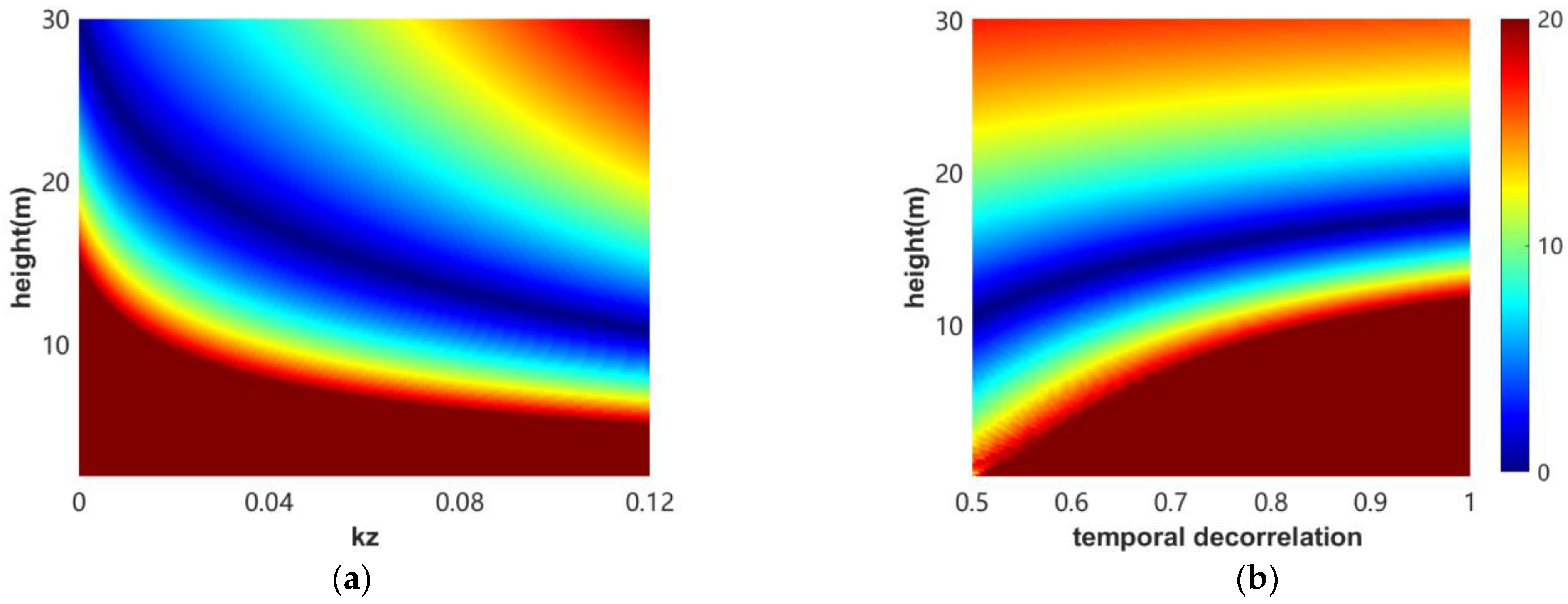
Since the semi-empirical improved RVoG model adopted in this study is based on the RvoG model and was used to empirically correct the effects of $k_z$ and temporal decorrelation, simulation experiments were conducted to further reveal the effects of $k_z$ and temporal decorrelation on the accuracy of forest height inversion. According to previous studies, the best $k_z$ range for estimating the forest height is between 0.06 and 0.1 rad/m [20]. When $k_z$ is less than 0.06 rad/m, the range of the interference coherence and coherence matrix ratio of the data is small, and the independence and decorrelation of the data are poor. When $k_z$ is greater than 0.1 rad/m, the error will further increase, which may lead to unreliable results [61]. Therefore, only the influence of $k_z$ variation in the range of 0–0.12 rad/m on the inversion accuracy of the tree height is considered. The estimated height error based on the RvoG model is simulated by fixed temporal decorrelation, together with the $k_z$ and $\sigma$ values (Figure 16). For all the $k_z$ values, temporal decorrelation leads to the overestimation (underestimation) of short (high) forests. In most cases, the degree of overestimation or underestimation varies with the forest height and $k_z$. However, in a specific range of forest heights, a better retrieval accuracy can be obtained, and this range varies with the $k_z$ value. With a fixed $\sigma$ of 0.15 dB/m and a temporal decorrelation of 0.98, a $k_z$ of 0.10 rad/m produces an error of less than 10%, but only when the forest height ranges from 8 to 23 m. The forest height range changes to 10–30 m when $k_z$ is 0.06 rad/m (Figure 16a). Therefore, a small $k_z$ value is more suitable for tall forests, while there will be obvious errors in the case of short vegetation. A large $k_z$ value is suitable for low vegetation, a finding which mirrors the existing research results [33]. By increasing the contribution of temporal decorrelation, the height range is rapidly reduced with good accuracy (Figure 16b). High vegetation is highly affected and serious estimation errors will occur if the temporal decorrelation increases further. According to the simulation results, it is necessary to adopt an appropriate $k_z$ and temporal decorrelation correction to achieve 20% accuracy in the height range of 0–30 m [19,37].

In this study, we found that as the temporal baseline increases, the observed complex coherence phase changes more than the coherence decreases. The combined effect of temporal decorrelation and volume decorrelation results in an inhomogeneous distribution of coherence in the same image. The error of the inversion results can be regulated within a relatively small range when the temporal decorrelation of the same data is established as a complex parameter. Due to the different forest heights and coherence conditions among the different elements in the same image, there are various constraints on the magnitude of the correction term. Therefore, using the same correction term inevitably leads to inconsistent parameter effects with different pixel values, and the influence of temporal decorrelation is not completely eliminated by semi-empirical iteration.

6.4. Future Work

Considering that the environment and the distribution of trees in different forest stands are variable and influenced by different degrees of wind-induced canopy movement and dielectric constant changes, the changes in the number of scatterers and changes in the dielectric constant caused by changes in the vegetation cover and water content have different effects on the temporal decorrelation of each sample plot. Therefore, by analyzing the relationship between each correction factor of each plot and the vegetation cover change and canopy water content and assigning a temporal decorrelation correction factor to each sample plot, we can effectively obtain high-precision forest height inversion results. However, the complex relationship between each correction coefficient and the influencing factors, such as temporal decorrelation and the forest structure, has not yet been found. Thus, it is not possible to conduct large-scale tree height inversion analysis and accurate regional-scale extrapolation work. In addition, the interference phase histogram used in this study to determine the vertical reflectance profile is based on the assumption that the normalized vertical structures of the trees in the forest are similar in a certain spatial domain. Therefore, the vertical structure profile of a single pixel cannot be estimated, and the effect of the forest stand density on the extinction coefficient is overlooked. Currently, our team is actively working on relevant data analysis and model improvements, attempting to use other methods to achieve the vertical profile fitting of each pixel, and exploring the correlation between forest structure parameters and temporal decorrelation correction factors to achieve high-precision regional forest height inversion.

7. Conclusions

In this paper, the empirical iterative model was used to correct the temporal decorrelation errors generated by satellite-based data, which effectively enabled us to avoid the loss of the traditional RVoG model’s capability for forest height inversion caused by the effects of the vertical wavenumber and temporal decorrelation. It was found that the extinction effect was significantly influenced by the forest stand density and forest height, and the introduction of an extinction coefficient that varies with height can effectively reduce the difference in the non-volume decorrelation response caused by the fixed extinction coefficient in the model. The results showed that the GVR is affected by the forest stand density, and in general the combination of the RVoG and PolInSAR decomposition techniques can improve the estimated results of the ground-only and volume-only complex coherence and, to some extent avoid the effect of excessive ground scattering in sparsely vegetated areas. In this study, repeat-pass spaceborne L-band ALOS-2 PALSAR data were used to perform forest height inversion on coniferous forests in the Saihanba Forest area, achieving a high inversion accuracy and improving the accuracy and robustness of the forest height inversion with long temporal baseline PolInSAR data. However, the objects of this study were all artificial coniferous forests and the influence of the forest stand density on the extinction effect was overlooked. Therefore, the capacity of the high-precision inversion method to assess the height of other heterogeneous forests requires further research and analysis.

References

1. Oliveira, C.P.D.; Ferreira, R.L.C.; da Silva, J.A.A.; Lima, R.B.D.; Silva, E.A.; Silva, A.F.D.; Lucena, J.D.S.D.; dos Santos, N.A.T.; Lopes, I.J.C.; Pessoa, M.M.D.L.; et al. Modeling and Spatialization of Biomass and Carbon Stock Using LiDAR Metrics in Tropical Dry Forest. Brazil. For. 2021, 12, 473. [Google Scholar] [CrossRef]
2. Chen, W.; Zheng, Q.; Xiang, H.; Chen, X.; Sakai, T. Forest Canopy Height Estimation Using Polarimetric Interferometric Synthetic Aperture Radar (PolInSAR) Technology Based on Full-Polarized ALOS/PALSAR Data. Remote Sens. 2021, 13, 174. [Google Scholar] [CrossRef]
3. Schlund, M.; Baron, D.; Magdon, P.; Erasmi, S. Canopy penetration depth estimation with TanDEM-X and its compensation in temperate forests. ISPRS J. Photogramm. Remote Sens. 2019, 147, 232–241. [Google Scholar] [CrossRef]
4. Lu, D.; Chen, Q.; Wang, G.; Liu, L.; Li, G.; Moran, E. A survey of remote sensing-based aboveground biomass estimation methods in forest ecosystems. Int. J. Digit. Earth 2014, 9, 63–105. [Google Scholar] [CrossRef]
5. Fu, W.; Guo, H.; Li, X.; Tian, B.; Sun, Z. Extended Three-Stage Polarimetric SAR Interferometry Algorithm by Dual-Polarization Data. IEEE Trans. Geosci. Remote Sens. 2015, 54, 2792–2802. [Google Scholar] [CrossRef]
6. Tan, L.; Yang, R. Investigation on Tree Height Retrieval with Polarimetric SAR Interferometry. In Proceedings of the IGARSS 2008—2008 IEEE International Geoscience and Remote Sensing Symposium, Boston, MA, USA, 7–11 July 2008; Volume 5, pp. 546–549. [Google Scholar] [CrossRef]
7. Eini-Zinab, S.; Maghsoudi, Y.; Sayedain, S.A. Assessing the performance of indicators resulting from three-component Freeman–Durden polarimetric SAR interferometry decomposition at P-and L-band in estimating tropical forest aboveground biomass. Int. J. Remote Sens. 2019, 41, 433–454. [Google Scholar] [CrossRef]
8. Berninger, A.; Lohberger, S.; Zhang, D.; Siegert, F. Canopy Height and Above-Ground Biomass Retrieval in Tropical Forests Using Multi-Pass X- and C-Band Pol-InSAR Data. Remote Sens. 2019, 11, 2105. [Google Scholar] [CrossRef] [Green Version]
9. Papathanassiou, K.; Cloude, S.R. Single Baseline Polarimetric SAR Interferometry. IEEE Trans. Geosci. Remote Sens. 2001, 39, 2352–2363. [Google Scholar] [CrossRef] [Green Version]
10. Managhebi, T.; Maghsoudi, Y.; Valadan Zoej, M.J. A new algorithm for forest height estimation based on the varied extinction random volume over ground (VERVoG) model using PolInSAR data. Int. J. Remote Sens. 2019, 41, 615–631. [Google Scholar] [CrossRef]
11. Managhebi, T.; Maghsoudi, Y.; Valadan Zoej, M.J. Four-Stage Inversion Algorithm for Forest Height Estimation Using Repeat Pass Polarimetric SAR Interferometry Data. Remote Sens. 2018, 10, 1174. [Google Scholar] [CrossRef] [Green Version]
12. Cloude, S.R.; Papathanassiou, K.P. Three-stage inversion process for polarimetric SAR interferometry. Radar, Sonar and Navigation. IEE Proc.-Radar Sonar Navig. 2003, 150, 125–134. [Google Scholar] [CrossRef] [Green Version]
13. Managhebi, T.; Maghsoudi, Y.; Valadan Zoej, M.J. A Volume Optimization Method to Improve the Three-Stage Inversion Algorithm for Forest Height Estimation Using PolInSAR Data. IEEE Geosci. Remote Sens. Lett. 2018, 15, 1214–1218. [Google Scholar] [CrossRef]
14. Lavalle, M.; Hensley, S. Extraction of Structural and Dynamic Properties of Forests From Polarimetric-Interferometric SAR Data Affected by Temporal Decorrelation. IEEE Trans. Geosci. Remote Sens. 2015, 53, 4752–4767. [Google Scholar] [CrossRef]
15. Papathanassiou, K.; Kugler, F.; Lee, S.; Marotti, L.; Hajnsek, I. Recent Advances in Polarimetric SAR Interferometry for Forest Parameter Estimation. In Proceedings of the 2008 IEEE Radar Conference, Rome, Italy, 26–30 May 2008; pp. 1–6. [Google Scholar] [CrossRef]
16. Lavalle, M.; Simard, M.; Pottier, E.; Solimini, D. PolinSAR forestry applications improved by modeling height dependent temporal decorrelation. In Proceedings of the 2010 IEEE International Geoscience and Remote Sensing Symposium, Honolulu, HI, USA, 25–30 July 2010; pp. 4772–4775. [Google Scholar] [CrossRef]
17. Lei, Y.; Siqueira, P. An Automatic Mosaicking Algorithm for the Generation of a Large-Scale Forest Height Map Using Spaceborne Repeat-Pass InSAR Correlation Magnitude. Remote Sens. 2015, 7, 5639–5659. [Google Scholar] [CrossRef] [Green Version]
18. Ahmed, R.; Siqueira, P.; Hensley, S.; Chapman, B.; Bergen, K. A survey of temporal decorrelation from spaceborne L-Band repeat-pass InSAR. Remote Sens. Environ. 2011, 115, 2887–2896. [Google Scholar] [CrossRef]
19. Kugler, F.; Lee, S.-K.; Hajnsek, I.; Papathanassiou, K. Forest Height Estimation by Means of Pol-InSAR Data Inversion: The Role of the Vertical Wavenumber. IEEE Trans. Geosci. Remote Sens. 2015, 53, 5294–5311. [Google Scholar] [CrossRef]
20. Du, K.; Lin, H.; Wang, G.; Jiangping, L.; Li, J.; Liu, Z. The Impact of Vertical Wavenumber on Forest Height Inversion by PolInSAR. In Proceedings of the 2018 Fifth International Workshop on Earth Observation and Remote Sensing Applications (EORSA), Xi’an, China, 18–20 June 2018; pp. 1–5. [Google Scholar] [CrossRef]
21. Fu, W.; Guo, H.; Song, P.; Tian, B.; Li, X.; Sun, Z. Combination of PolInSAR and LiDAR techniques for forest height estimation. IEEE Geosci. Remote Sens. Lett. 2017, 14, 1218–1222. [Google Scholar] [CrossRef]
22. Managhebi, T.; Maghsoudi, Y.; Valadan Zoej, M.J. An Improved Three-Stage Inversion Algorithm in Forest Height Estimation Using Single-Baseline Polarimetric SAR Interferometry Data. IEEE Geosci. Remote Sens. Lett. 2018, 15, 887–891. [Google Scholar] [CrossRef]
23. Garestier, F.; Le Toan, T. Forest modeling for height inversion using single-baseline InSAR/Pol-InSAR data. IEEE Trans. Geosci. Remote Sens. 2010, 48, 1528–1539. [Google Scholar] [CrossRef]
24. Balzter, H.; Rowland, C.S.; Saich, P. Forest canopy height and carbon estimation at Monks Wood National Nature Reserve, UK, using dual-wavelength SAR interferometry. Remote Sens. Environ. 2007, 108, 224–239. [Google Scholar] [CrossRef]
25. Liao, Z.; He, B.; Quan, X.; van Dijk, A.; Qiu, S.; Yin, C. Biomass estimation in dense tropical forest using multiple information from single-baseline P-band PolInSAR data. Remote Sens. Environ. 2019, 221, 489–507. [Google Scholar] [CrossRef]
26. Aghabalaei, A.; Ebadi, H.; Maghsoudi, Y. Forest height estimation based on the RVoG inversion model and the PolInSAR decomposition technique. Int. J. Remote Sens. 2019, 41, 2684–2703. [Google Scholar] [CrossRef]
27. Yamada, H.; Yamaguchi, Y.; Sato, R. Polarimetric Scattering Model Decomposition for Pol-InSAR Data. In Proceedings of the IEEE International Geoscience and Remote Sensing Symposium, Boston, MA, USA, 7–11 July 2008; Volume 4, pp. 331–334. [Google Scholar] [CrossRef]
28. Joshi, S.; Kumar, S. Performance of PolSAR backscatter and PolInSAR coherence for scattering characterization of forest vegetation using single pass X-band spaceborne synthetic aperture radar data. J. Appl. Remote Sens. 2017, 11, 026022. [Google Scholar] [CrossRef]
29. Ballester-Berman, J.D.; Lopez-Sanchez, J. Applying the Freeman–Durden Decomposition Concept to Polarimetric SAR Interferometry. IEEE Trans. Geosci. Remote Sens. 2010, 48, 466–479. [Google Scholar] [CrossRef]
30. Chen, A.; Zebker, H. Reducing Ionospheric Effects in InSAR Data Using Accurate Coregistration. IEEE Trans. Geosci. Remote Sens. 2014, 52, 60–70. [Google Scholar] [CrossRef]
31. Jung, J.; Kim, D.-j.; Lavalle, M.; Yun, S.-H. Coherent Change Detection Using InSAR Temporal Decorrelation Model: A Case Study for Volcanic Ash Detection. IEEE Trans. Geosci. Remote Sens. 2016, 54, 5765–5775. [Google Scholar] [CrossRef]
32. Rosen, P.; Hensley, S.; Joughin, I.R.; Li, F.K.; Madsen, S.; Rodriguez, E.; Goldstein, R.M. Synthetic Aperture Radar Interferometry. Proc. IEEE 2000, 88, 333–382. [Google Scholar] [CrossRef]
33. Liao, Z.; He, B.; van Dijk, A.; Bai, X.; Quan, X. The impacts of spatial baseline on forest canopy height model and digital terrain model retrieval using P-band PolInSAR data. Remote Sens. Environ. 2018, 210, 403–421. [Google Scholar] [CrossRef]
34. Tahraoui, S.; Ouarzeddine, M. Assess the Effects of Wind on Forest Parameters Inversion by Using Pol-InSAR Applications. In Advanced Control Engineering Methods in Electrical Engineering Systems; Lecture Notes in Electrical Engineering; Springer International Publishing: Berlin/Heidelberg, Germany, 2019; Volume 522, pp. 556–564. [Google Scholar] [CrossRef]
35. Yadav, S.; Padalia, H.; Sinha, S.K.; Srinet, R.; Chauhan, P. Above-ground biomass estimation of Indian tropical forests using X band Pol-InSAR and Random Forest. Remote Sens. Appl. Soc. Environ. 2021, 21, 100462. [Google Scholar] [CrossRef]
36. Lei, Y.; Siqueira, P. Estimation of Forest Height Using Spaceborne Repeat-Pass L-Band InSAR Correlation Magnitude over the US State of Maine. Remote Sens. 2014, 6, 10252–10285. [Google Scholar] [CrossRef] [Green Version]
37. Mao, Y.; Michel, O.; Yu, Y.; Fan, W.; Sui, A.; Liu, Z.; Wu, G. Retrieval of Boreal Forest Heights Using an Improved Random Volume over Ground (RVoG) Model Based on Repeat-Pass Spaceborne Polarimetric SAR Interferometry: The Case Study of Saihanba, China. Remote Sens. 2021, 13, 4306. [Google Scholar] [CrossRef]
38. Praks, J.; Antropov, O.; Hallikainen, M.T. LIDAR-Aided SAR Interferometry Studies in Boreal Forest: Scattering Phase Center and Extinction Coefficient at X- and L-Band. IEEE Trans. Geosci. Remote Sens. 2012, 50, 3831–3843. [Google Scholar] [CrossRef]
39. Lee, S.-K.; Fatoyinbo, L. TanDEM-X Pol-InSAR Inversion for Mangrove Canopy Height Estimation. IEEE J. Sel. Top. Appl. Earth Obs. Remote Sens. 2015, 8, 3608–3618. [Google Scholar] [CrossRef]
40. Cloude, S. Polarization coherence tomography. Radio Sci. 2006, 41, 1–27. [Google Scholar] [CrossRef]
41. Sun, G.; Ranson, K.J.; Kimes, D.; Blair, J.; Kovacs, K. Forest vertical structure from GLAS: An evaluation using LVIS and SRTM data. Remote Sens. Environ. 2008, 112, 107–117. [Google Scholar] [CrossRef]
42. Choi, C.; Pardini, M.; Heym, M.; Papathanassiou, K. Improving Forest Height-to-Biomass Allometry with Structure Information: A TanDEM-X Study. IEEE J. Sel. Top. Appl. Earth Obs. Remote Sens. 2021, 14, 10415–10427. [Google Scholar] [CrossRef]
43. Garestier, F.; Dubois-Fernandez, P.; Champion, I.; Le Toan, T. Pine forest investigation using high resolution P-band Pol-InSAR data. Remote Sens. Environ. 2011, 115, 2897–2905. [Google Scholar] [CrossRef]
44. Cui, Y.; Yamaguchi, Y.; Yang, J.; Park, S.-E.; Kobayashi, H.; Singh, G. Three-Component Power Decomposition for Polarimetric SAR Data Based on Adaptive Volume Scatter Modeling. Remote Sens. 2012, 4, 1559–1572. [Google Scholar] [CrossRef] [Green Version]
45. Jiangping, L.; Lin, H.; Wang, G.; Sun, H.; Yan, E. Mapping Growing Stem Volume of Chinese Fir Plantation Using a Saturation-based Multivariate Method and Quad-polarimetric SAR Images. Remote Sens. 2019, 11, 1872. [Google Scholar] [CrossRef] [Green Version]
46. Wang, C.; Wang, L.; Fu, H.; Xie, Q.; Zhu, J. The Impact of Forest Density on Forest Height Inversion Modeling from Polarimetric InSAR Data. Remote Sens. 2016, 8, 291. [Google Scholar] [CrossRef] [Green Version]
47. Cloude, S.R.; Papathanassiou, K.P. Polarimetric SAR interferometry. IEEE Trans. Geosci. Remote Sens. 1998, 36, 1551–1565. [Google Scholar] [CrossRef]
48. Ferro-Famil, L.; Reigber, A.; Pottier, E.; Boerner, W.M. Scene characterization using subaperture polarimetric SAR data. IEEE Trans. Geosci. Remote Sens. 2003, 41, 2264–2276. [Google Scholar] [CrossRef]
49. Ferro-Famil, L.; Neumann, M. Recent Advances in the Derivation of PolInSAR Statistics: Study and Application. In Proceedings of the 7th European Conference on Synthetic Aperture Radar, Friedrichshafen, Germany, 2–5 June 2008; pp. 1–4. [Google Scholar]
50. Neumann, M.; Ferro-Famil, L.; Reigber, A. Estimation of Forest Structure, Ground, and Canopy Layer Characteristics From Multibaseline Polarimetric Interferometric SAR Data. IEEE Trans. Geosci. Remote Sens. 2010, 48, 1086–1104. [Google Scholar] [CrossRef] [Green Version]
51. Ni, W.; Zhang, Z.; Sun, G.; Liu, Q. Modeling Interferometric SAR Features of Forest Canopies Over Mountainous Area at Landscape Scales. IEEE Trans. Geosci. Remote Sens. 2018, 56, 2958–2967. [Google Scholar] [CrossRef]
52. Thirion-Lefevre, L.; Colin-Koeniguer, E. Investigating Attenuation, Scattering Phase Center, and Total Height Using Simulated Interferometric SAR Images of Forested Areas. IEEE Trans. Geosci. Remote Sens. 2007, 45, 3172–3179. [Google Scholar] [CrossRef]
53. Lucas, R.; Reid, N.; Lee, A.; Moghaddam, M.; Witte, C.; Tickle, P. Empirical relationships between AIRSAR backscatter and LiDAR-derived forest biomass, Queensland. Australia. Remote Sens. Environ. 2006, 100, 407–425. [Google Scholar] [CrossRef]
54. Hussin, Y.A.; Reich, R.M.; Hoffer, R.M. Estimating splash pine biomass using radar backscatter. IEEE Trans. Geosci. Remote Sens. 1991, 29, 427–431. [Google Scholar] [CrossRef]
55. Hagberg, J.O.; Ulander, L.M.H.; Askne, J. Repeat-pass SAR interferometry over forested terrain. IEEE Trans. Geosci. Remote Sens. 1995, 33, 331–340. [Google Scholar] [CrossRef]
56. Hill, M.; Ticehurst, C.; Lee, J.-S.; Grunes, M.; Donald, G.; Henry, D. Integration of optical and radar classifications for mapping pasture type in Western Australia. IEEE Trans. Geosci. Remote Sens. 2005, 43, 1665–1681. [Google Scholar] [CrossRef]
57. Parache, H.; Mayer, T.; Herndon, K.; Flores-Anderson, A.; Lei, Y.; Nguyen, Q.; Kunlamai, T.; Griffin, R. Estimating Forest Stand Height in Savannakhet, Lao PDR Using InSAR and Backscatter Methods with L-Band SAR Data. Remote Sens. 2021, 13, 4516. [Google Scholar] [CrossRef]
58. Shiroma, G.; Lavalle, M. Digital Terrain, Surface, and Canopy Height Models From InSAR Backscatter-Height Histograms. IEEE Trans. Geosci. Remote Sens. 2020, 58, 3754–3777. [Google Scholar] [CrossRef]
59. Khati, U.; Lavalle, M.; Singh, G. Spaceborne tomography of multi-species Indian tropical forests. Remote Sens. Environ. 2019, 229, 193–212. [Google Scholar] [CrossRef]
60. Fu, H.; Wang, C.; Jian-Jun, Z.; Xie, Q.; Zhang, B. Estimation of pine forest height and underlying DEM using multi-baseline P-band PolInSAR data. Remote Sens. 2016, 8, 820. [Google Scholar] [CrossRef] [Green Version]
61. Shi, Y.; He, B.; Liao, Z. An improved dual-baseline PolInSAR method for forest height inversion. Int. J. Appl. Earth Obs. Geoinf. 2021, 103, 102483. [Google Scholar] [CrossRef]
Figure 1. The map of the study area. The area is located in the Saihanba Forest, China. The distribution of the real sample locations is indicated by the red dots. The image of the study area is derived from SAR data under HV polarization.
Remotesensing 15 01272 g001
Figure 2. Relationship between the forest structure parameters at the plot level. (a) Mean DBH vs. mean tree height, (b) mean DBH vs. forest stand density and (c) mean tree height vs. mean canopy thickness.
Remotesensing 15 01272 g002
Figure 3. (a) HV polarization coherence image. (b) The local incidence angle. (c) The vertical wavenumber of the 0711-0725 interference pair obtained after image preprocessing.
Remotesensing 15 01272 g003
Figure 4. The RVoG inversion model.
Remotesensing 15 01272 g004
Figure 5. Flowchart of the proposed method employed in this study.
Remotesensing 15 01272 g005
Figure 6. Fitting scatterplot of the inverse tree height in relation to the measured height for the original model and the improved model. The 1:1 line is in blue and the fitted curve is in green. The horizontal axis (True) is the measured tree height, the vertical axis (PolInSAR) is the model fitting result, R2 and RMSE are the coefficient of determination and root mean square error, respectively.
Remotesensing 15 01272 g006
Figure 7. The inversion forest height images.
Remotesensing 15 01272 g007
Figure 8. Comparative diagram of complex coherence before and after applying the improved extinction coefficient. The interference coherence on the complex plane is represented as a random volume in red, with h v of 0–30 m. In (a,b), the constant extinction coefficient values and the extinction coefficient influencing factor values of 0.01, 0.2, 0.5 and 1 dB/m are shown in purple, blue, yellow and green, respectively. In (a), the red segment is the RVoG model corresponding to the given constant extinction random volume height, and in (b), the red segment is the semi-empirical improved RVoG inversion model corresponding to the given extinction coefficient influence factor random volume height.
Remotesensing 15 01272 g008
Figure 9. Volume coherence and interference phase plots obtained for different extinction coefficients. (a) Volume coherence and height diagram with different extinction coefficients. (b) Interference phase and height diagram with different extinction coefficients. The fixed extinction coefficients (0.01 and 1 dB/m) are represented by black dots, and the extinction coefficient influence factors (0.01, 0.2, 0.5 and 1 dB/m) are represented in blue, green, yellow and red, respectively.
Remotesensing 15 01272 g009
Figure 10. Schematic diagram of the penetration depth.
Remotesensing 15 01272 g010
Figure 11. Diagram of the relationship between the extinction coefficient and the penetration depth, where the extinction coefficient is considered to be the attenuation coefficient and reciprocal of the penetration depth. (a) Penetration depth vs. extinction coefficient (the shade of the scatter color is the magnitude of the forest height). (b,c) are the scatter relationship diagrams of the mean tree height and the penetration depth and the extinction coefficient of HH, HV and VV polarization, respectively. (d) Mean canopy thickness vs. extinction coefficient (the shade of the scatter color is the magnitude of penetration depth). (e) Mean DBH vs. extinction coefficient (the shade of the scatter color is the magnitude of the penetration depth).
Remotesensing 15 01272 g011
Figure 12. (a): Vertical reflectance profile fitted by the InSAR phase center height histogram and Gaussian function. The histogram reflecting the vertical reflectance profile is red, and the vertical reflectance profile obtained by Gaussian function fitting is blue. The vertical axis shows the normalization of the forest heights ranging from 0 to 1 m. (b): Change in the magnitude of the influence factor a for different extinction coefficients, which determine the shape of the curve. The curves of 0.2, 0.5 and 1 for a are indicated in blue, red and green, respectively, and the a value obtained by fitting the Gaussian function is yellow.
Remotesensing 15 01272 g012
Figure 13. (a) Forest height deviation map based on the assumption of zero GVR and (b) the histogram of GVR after the improvement of the 0711-0725 interference pairs.
Remotesensing 15 01272 g013
Figure 14. Fifteen common complex coherences (HH, HV, VV, HHVV, HH + VV, HH − VV, HV + VH, LL, LR, RR, Opt1, Opt2, Opt3, PD High, PD Low) and the complex coherences ( γ G , γ V ) obtained in this study were used for the comparison of GVR at low and high forest stand densities. Left: low density; right: high density.
Remotesensing 15 01272 g014
Figure 15. Linear plot of the GVR and stand density.
Remotesensing 15 01272 g015
Figure 16. The forest height is relative to the retrieved the error and is defined as h v h t r u e / h t r u e × 100 % , with a range of 0% to 20%. (a): The fixed temporal decorrelation is 0.98, and the error of the tree height of 0–30 m when k z is 0–0.12 is analyzed. (b): Fix k z = 0.1 and analyze the error variation of the 0–30 m tree height in the range of 0.5–1 for temporal decorrelation.
Remotesensing 15 01272 g016