


Automatic Segmentation of Water Bodies Using RGB Data: A Physically Based Approach


Abstract
1. Introduction
2. Materials and Methods
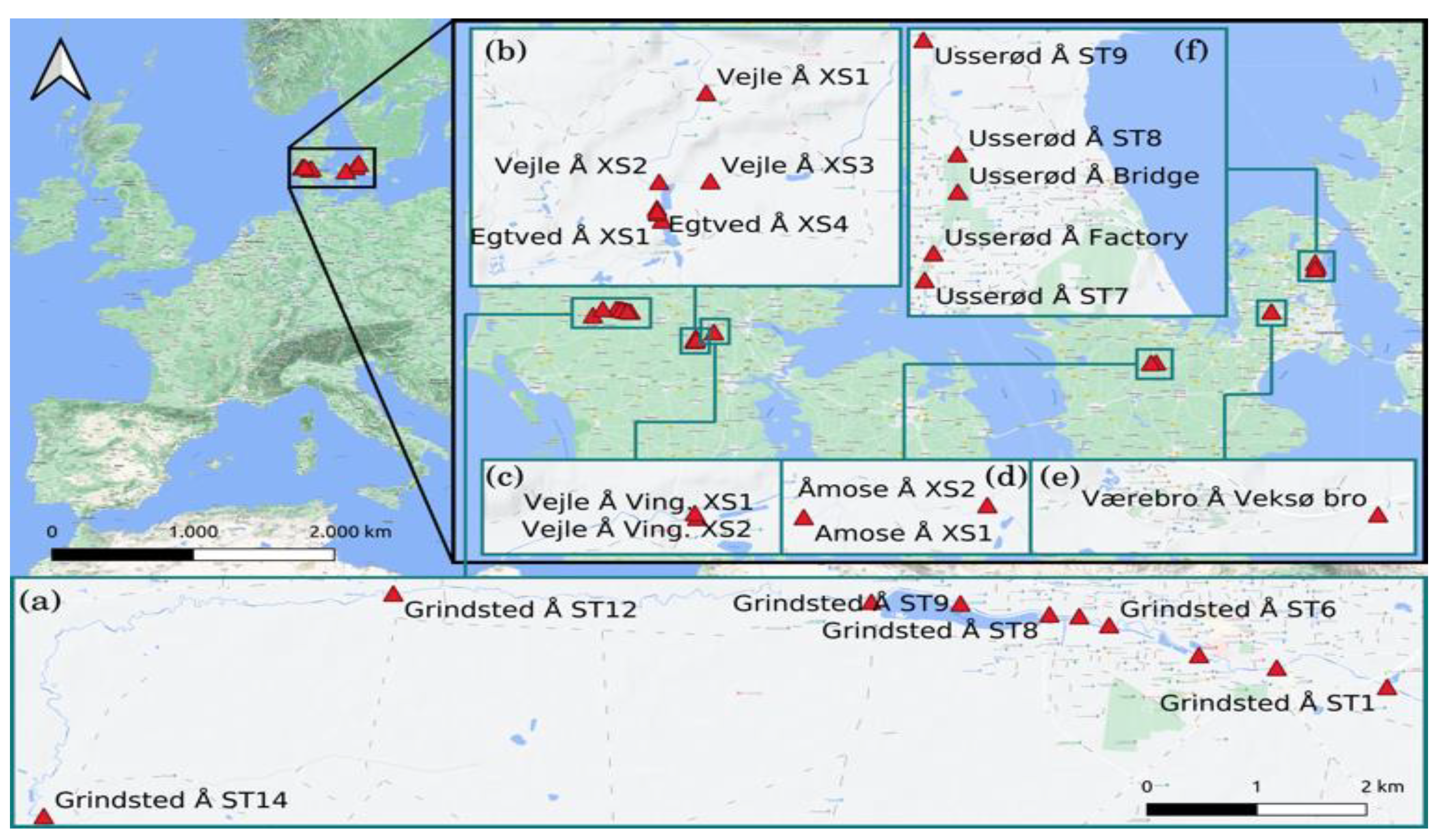
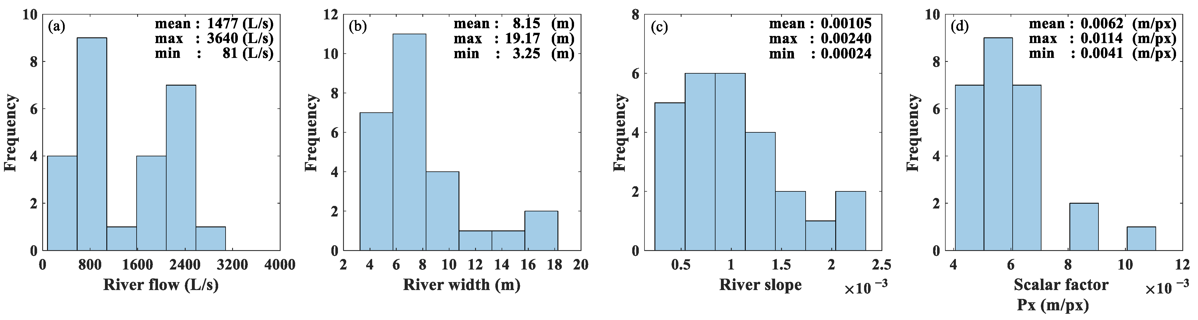
2.1. Case Studies
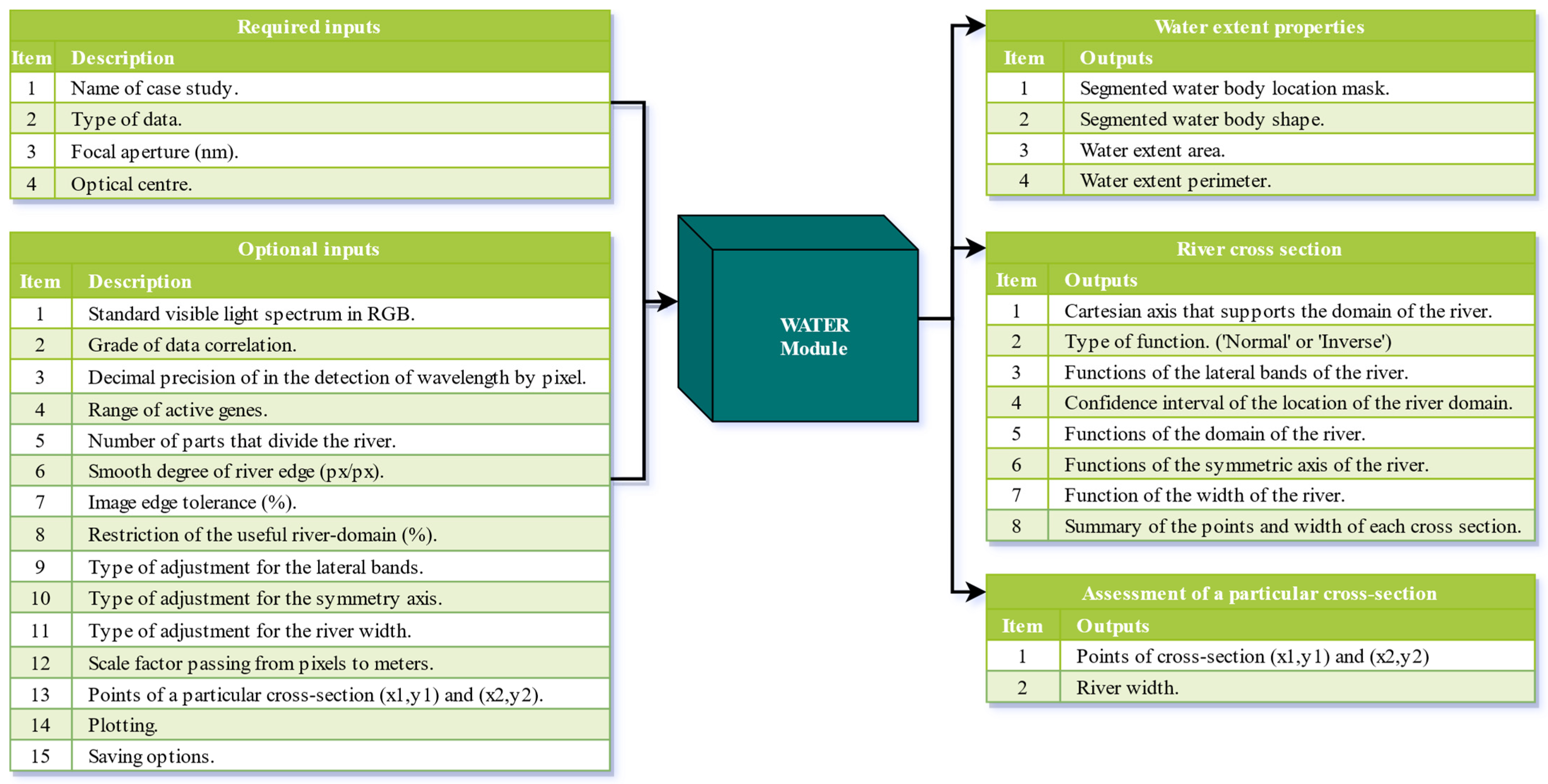
2.2. WATER Overview
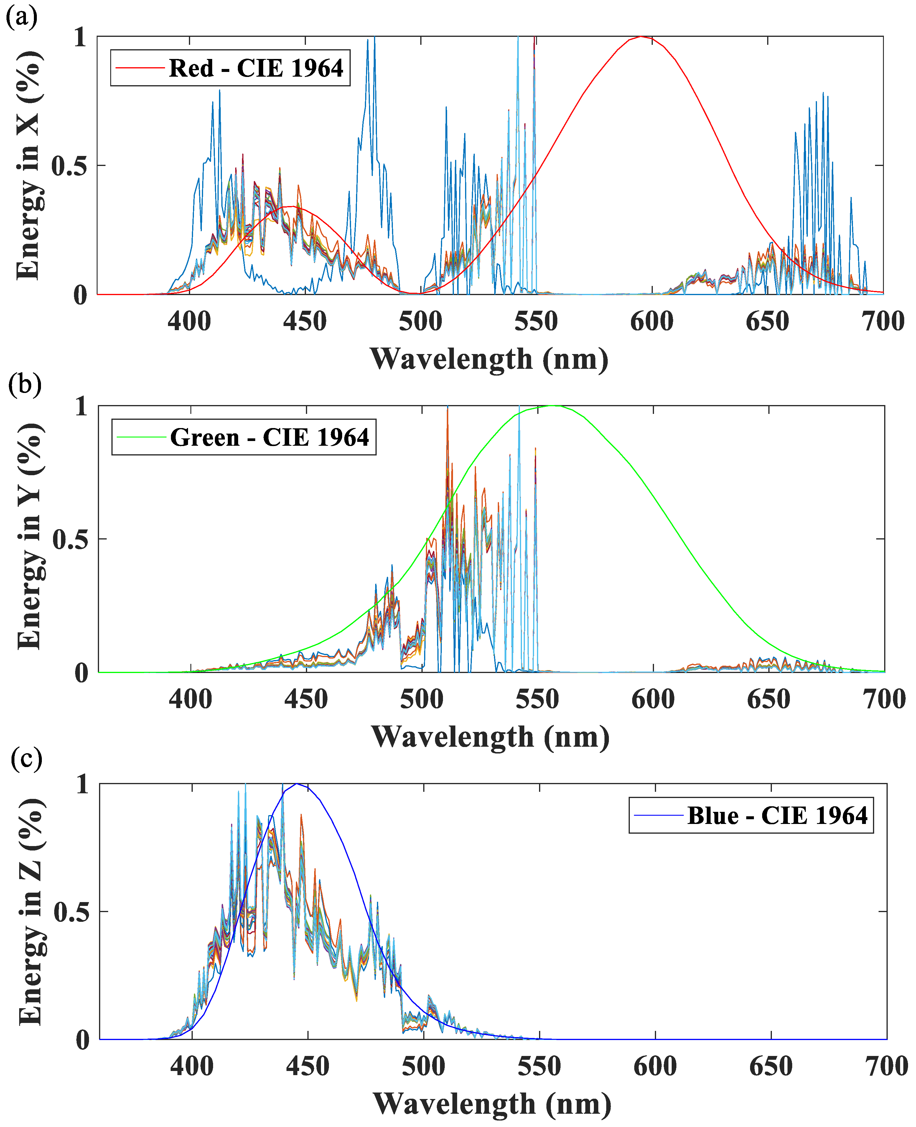
2.3. Performance of RGB Sensor
2.4. Single-Slit Diffraction Simulation
2.5. Reflectance Filter
2.6. Pseudo Genetic Algorithmic
2.7. Water Body Detection and Extracted Characteristics
3. Results
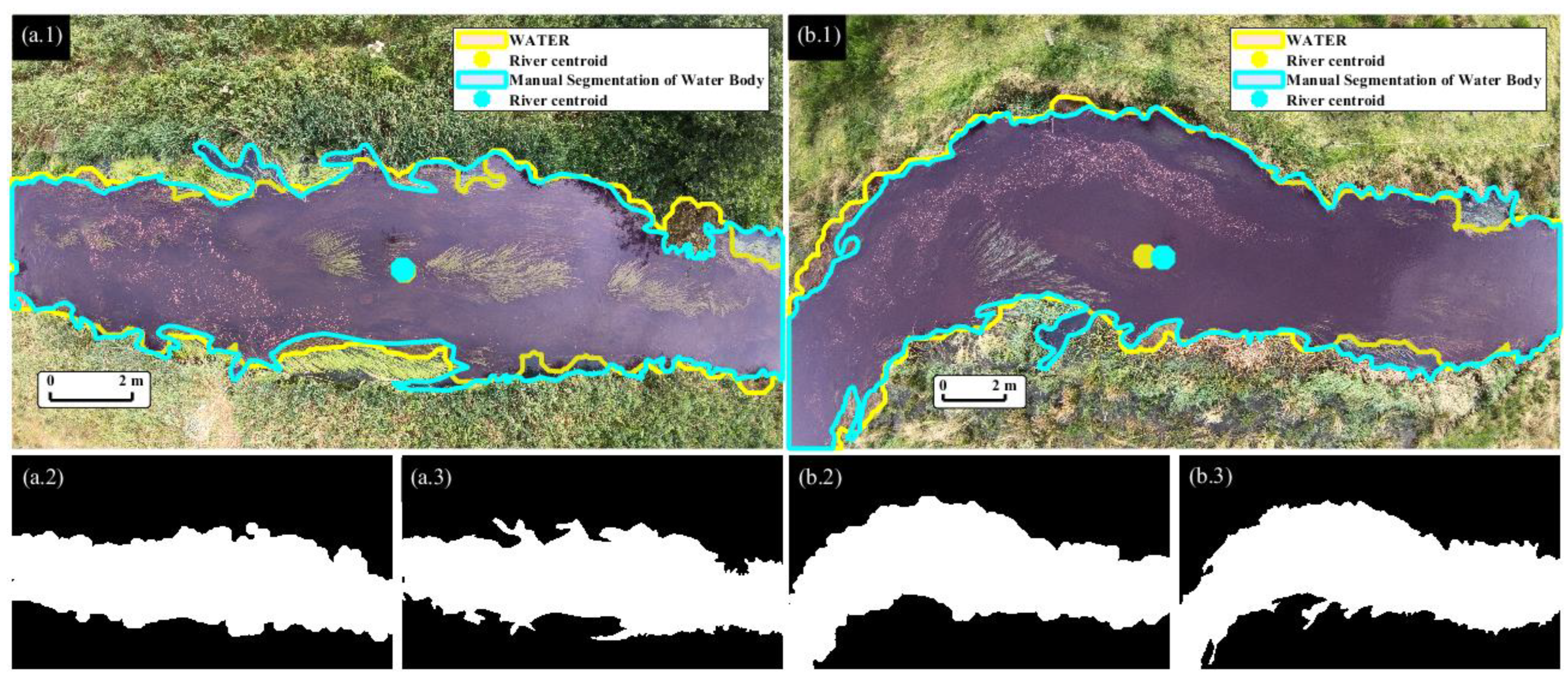
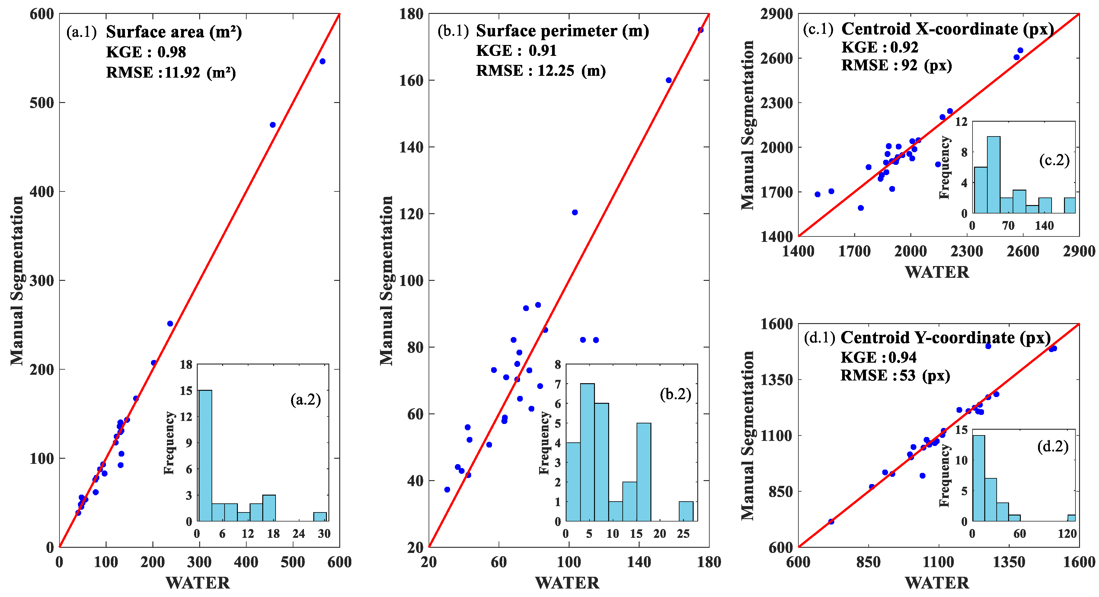
3.1. Automatic Versus Manually Based Water Segmentation
3.2. Processing Time
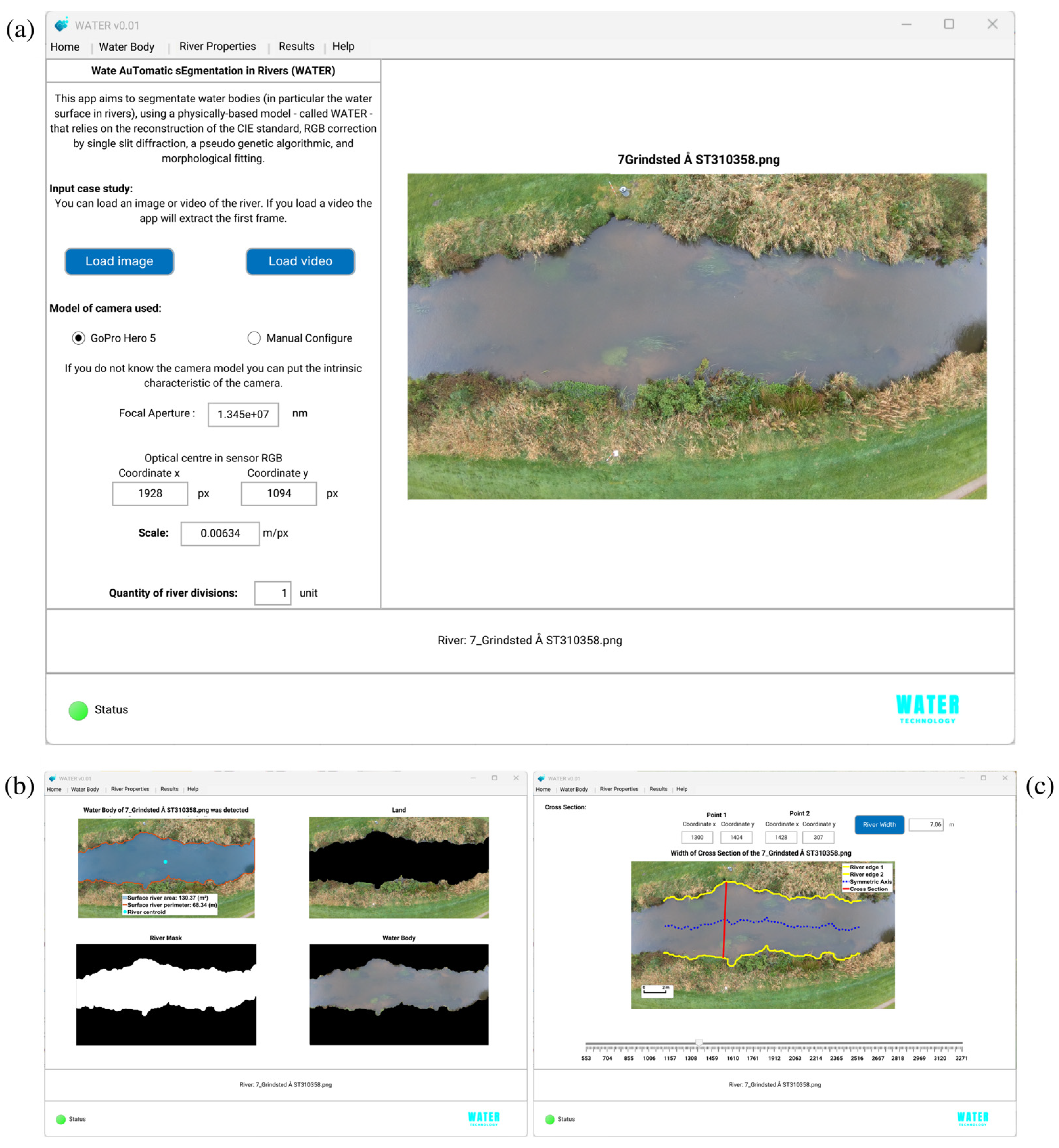
3.3. WATER v0.01 Software
4. Discussion
5. Conclusions
Supplementary Materials
Author Contributions
Funding
Data Availability Statement
Conflicts of Interest
References
- Freden, S.C.; Mercanti, E.P.; Becker, M.A. Third Earth Resources Technology Satellite-1 Symposium: Section A–B. Technical presentations; Scientific and Technical Information Office, National Aeronautics and Space Administration: Washington, DC, USA, 1973. [Google Scholar]
- McFeeters, S.K. The use of the Normalized Difference Water Index (NDWI) in the delineation of open water features. Int. J. Remote Sens. 1996, 17, 1425–1432. [Google Scholar] [CrossRef]
- Gao, B.-C. NDWI—A normalized difference water index for remote sensing of vegetation liquid water from space. Remote Sens. Environ. 1996, 58, 257–266. [Google Scholar] [CrossRef]
- Xu, H. Modification of normalised difference water index (NDWI) to enhance open water features in remotely sensed imagery. Int. J. Remote Sens. 2006, 27, 3025–3033. [Google Scholar] [CrossRef]
- Shen, L.; Li, C. Water body extraction from Landsat ETM+ imagery using adaboost algorithm. In Proceedings of the 2010 18th International Conference on Geoinformatics, Beijing, China, 18–20 June 2010; pp. 1–4. [Google Scholar] [CrossRef]
- Albertini, C.; Gioia, A.; Iacobellis, V.; Manfreda, S. Detection of Surface Water and Floods with Multispectral Satellites. Remote Sens. 2022, 14, 6005. [Google Scholar] [CrossRef]
- Akiyama, T.S.; Junior, J.M.; Gonçalves, W.N.; Bressan, P.O.; Eltner, A.; Binder, F.; Singer, T. Deep Learning Applied to Water Segmentation. Int. Arch. Photogramm. Remote Sens. Spat. Inf. Sci. 2020, XLIII-B2-2, 1189–1193. [Google Scholar] [CrossRef]
- Xia, M.; Cui, Y.; Zhang, Y.; Xu, Y.; Liu, J.; Xu, Y. DAU-Net: A novel water areas segmentation structure for remote sensing image. Int. J. Remote Sens. 2021, 42, 2594–2621. [Google Scholar] [CrossRef]
- Wan, H.L.; Jung, C.; Hou, B.; Wang, G.T.; Tang, Q.X. Novel Change Detection in SAR Imagery Using Local Connectivity. IEEE Geosci. Remote Sens. Lett. 2012, 10, 174–178. [Google Scholar] [CrossRef]
- Li, N.; Wang, R.; Liu, Y.; Du, K.; Chen, J.; Deng, Y. Robust river boundaries extraction of dammed lakes in mountain areas after Wenchuan Earthquake from high resolution SAR images combining local connectivity and ACM. ISPRS J. Photogramm. Remote Sens. 2014, 94, 91–101. [Google Scholar] [CrossRef]
- Yuan, X.; Sarma, V. Automatic Urban Water-Body Detection and Segmentation From Sparse ALSM Data via Spatially Constrained Model-Driven Clustering. IEEE Geosci. Remote Sens. Lett. 2010, 8, 73–77. [Google Scholar] [CrossRef]
- Ansari, E.; Akhtar, M.N.; Abdullah, M.N.; Othman, W.A.F.W.; Abu Bakar, E.; Hawary, A.F.; Alhady, S.S.N. Image Processing of UAV Imagery for River Feature Recognition of Kerian River, Malaysia. Sustainability 2021, 13, 9568. [Google Scholar] [CrossRef]
- Ronneberger, O.; Fischer, P.; Brox, T. U-Net: Convolutional Networks for Biomedical Image Segmentation. In Proceedings of the Medical Image Computing and Computer-Assisted Intervention–MICCAI 2015: 18th International Conference, Munich, Germany, 5–9 October 2015; Springer: Cham, Switzerland, 2015; pp. 234–241. [Google Scholar]
- Teichmann, M.T.T.; Cipolla, R. Convolutional CRFs for Semantic Segmentation. In Proceedings of the 30th British Machine Vision Conference 2019, Cardiff, UK, 9–12 September 2019. [Google Scholar] [CrossRef]
- Rankin, A.; Matthies, L. Daytime water detection and localization for unmanned ground vehicle autonomous navigation. In Proceedings of the 25th Army Science Conference, Orlando, FL, USA, 27–30 November 2006. [Google Scholar]
- Li, K.; Wang, J.; Yao, J. Effectiveness of machine learning methods for water segmentation with ROI as the label: A case study of the Tuul River in Mongolia. Int. J. Appl. Earth Obs. Geoinf. 2021, 103, 102497. [Google Scholar] [CrossRef]
- Sarwal, A.; Nett, J.; Simon, D. Detection of Small Water-Bodies; Perceptek Inc.: Littleton, CO, USA, 2004. [Google Scholar]
- Achar, S.; Sankaran, B.; Nuske, S.; Scherer, S.; Singh, S. Self-supervised segmentation of river scenes. In Proceedings of the 2011 IEEE International Conference on Robotics and Automation, Shanghai, China, 9–13 May 2011; pp. 6227–6232. [Google Scholar] [CrossRef]
- Zhang, X.; Jin, J.; Lan, Z.; Li, C.; Fan, M.; Wang, Y.; Yu, X.; Zhang, Y. ICENET: A Semantic Segmentation Deep Network for River Ice by Fusing Positional and Channel-Wise Attentive Features. Remote Sens. 2020, 12, 221. [Google Scholar] [CrossRef]
- Bandini, F.; Lüthi, B.; Peña-Haro, S.; Borst, C.; Liu, J.; Karagkiolidou, S.; Hu, X.; Lemaire, G.G.; Bjerg, P.L.; Bauer-Gottwein, P. A Drone-Borne Method to Jointly Estimate Discharge and Manning’s Roughness of Natural Streams. Water Resour. Res. 2021, 57, e2020WR028266. [Google Scholar] [CrossRef]
- Trezona, P.W. Derivation of the 1964 CIE 10° XYZ colour-matching functions and their applicability in photometry. Color Res. Appl. 2000, 26, 67–75. [Google Scholar] [CrossRef]
- Compton, A.H.; Heisenberg, W. The Physical Principles of the Quantum Theory; Springer: Berlin/Heidelberg, Germany, 1984. [Google Scholar] [CrossRef]
- Wu, E.T.H. Yangton and Yington-A Hypothetical Theory of Everything. Sci. J. Phys. 2015, 2013. [Google Scholar] [CrossRef]
- Wu, E.T.H. Single Slit Diffraction and Double Slit Interference Interpreted by Yangton and Yington Theory. IOSR J. Appl. Phys. 2020, 12. [Google Scholar] [CrossRef]
- Knight, P.L.; Bužek, V. Squeezed States: Basic Principles. Quantum Squeezing 2004, 27, 3–32. [Google Scholar] [CrossRef]
- Mancini, A.; Frontoni, E.; Zingaretti, P.; Longhi, S. High-resolution mapping of river and estuary areas by using unmanned aerial and surface platforms. In Proceedings of the 2015 International Conference on Unmanned Aircraft Systems (ICUAS), Denver, CO, USA, 9–12 June 2015; pp. 534–542. [Google Scholar] [CrossRef]
- Muhadi, N.A.; Abdullah, A.F.; Bejo, S.K.; Mahadi, M.R.; Mijic, A. Image Segmentation Methods for Flood Monitoring System. Water 2020, 12, 1825. [Google Scholar] [CrossRef]
- Harika, A.; Sivanpillai, R.; Variyar, V.V.S.; Sowmya, V. Extracting Water Bodies in Rgb Images Using Deeplabv3+ Algorithm. In The International Archives of Photogrammetry, Remote Sensing and Spatial Information Sciences; ISPRS: Gottingen, Germany, 2022; Volume XLVI-M-2–2022, pp. 97–101. [Google Scholar] [CrossRef]
- Erfani, S.M.H.; Wu, Z.; Wu, X.; Wang, S.; Goharian, E. ATLANTIS: A benchmark for semantic segmentation of waterbody images. Environ. Model. Softw. 2022, 149, 105333. [Google Scholar] [CrossRef]
- Zhou, Y.; Ren, D.; Emerton, N.; Lim, S.; Large, T. Image Restoration for Under-Display Camera. In Proceedings of the 2021 IEEE/CVF Conference on Computer Vision and Pattern Recognition (CVPR), Nashville, TN, USA, 20–25 June 2021; pp. 9175–9184. [Google Scholar] [CrossRef]
- Gamba, M.T.; Marucco, G.; Pini, M.; Ugazio, S.; Falletti, E.; Presti, L.L. Prototyping a GNSS-Based Passive Radar for UAVs: An Instrument to Classify the Water Content Feature of Lands. Sensors 2015, 15, 28287–28313. [Google Scholar] [CrossRef]
- Issa, H.; Stienne, G.; Reboul, S.; Raad, M.; Faour, G. Airborne GNSS Reflectometry for Water Body Detection. Remote Sens. 2021, 14, 163. [Google Scholar] [CrossRef]
- Imam, R.; Pini, M.; Marucco, G.; Dominici, F.; Dovis, F. UAV-Based GNSS-R for Water Detection as a Support to Flood Monitoring Operations: A Feasibility Study †. Appl. Sci. 2019, 10, 210. [Google Scholar] [CrossRef]
- Perez-Portero, A.; Munoz-Martin, J.F.; Park, H.; Camps, A. Airborne GNSS-R: A Key Enabling Technology for Environmental Monitoring. IEEE J. Sel. Top. Appl. Earth Obs. Remote Sens. 2021, 14, 6652–6661. [Google Scholar] [CrossRef]


| Characteristic | Item | Value | Unit |
|---|---|---|---|
| Focal aperture | 1.345 × 10⁷ | (nm) | |
| Optical centre Y | 1094 | (px) | |
| Optical centre X | 1928 | (px) |
| Area (m2) | Perimeter (m) | Centroid Coordinate X (px) | Centroid Coordinate Y (px) | |||||||||
|---|---|---|---|---|---|---|---|---|---|---|---|---|
| ID | WATER | Manual | Error | WATER | Manual | Error | WATER | Manual | Error | WATER | Manual | Error |
| 1 | 49.37 | 49.86 | −1.0% | 36 | 46 | −20.4% | 2009 | 2040 | −1.5% | 1304 | 1285 | 1.5% |
| 2 | 50.60 | 54.15 | −6.6% | 43 | 54 | −20.0% | 2209 | 2244 | −1.5% | 1056 | 1080 | −2.2% |
| 3 | 40.34 | 38.61 | 4.5% | 42 | 58 | −27.1% | 2585 | 2652 | −2.5% | 1173 | 1214 | −3.4% |
| 4 | 120.48 | 117.50 | 2.5% | 70 | 78 | −9.6% | 2041 | 2047 | −0.3% | 1246 | 1237 | 0.7% |
| 5 | 130.67 | 140.15 | −6.8% | 70 | 74 | −4.2% | 1875 | 1955 | −4.1% | 862 | 870 | −1.0% |
| 6 | 79.33 | 77.98 | 1.7% | 63 | 61 | 4.1% | 1868 | 1897 | −1.5% | 1227 | 1224 | 0.3% |
| 7 | 130.36 | 129.06 | 1.0% | 68 | 86 | −20.2% | 1899 | 1907 | −0.4% | 934 | 928 | 0.7% |
| 8 | 96.69 | 82.71 | 16.9% | 72 | 82 | −12.7% | 1900 | 1720 | 10.5% | 909 | 935 | −2.8% |
| 9 | 163.92 | 167.01 | −1.9% | 64 | 74 | −13.6% | 2007 | 1925 | 4.3% | 997 | 1015 | −1.8% |
| 10 | 202.37 | 182.83 | 10.7% | 108 | 111 | −3.1% | 2565 | 2606 | −1.6% | 1010 | 1072 | −5.8% |
| 11 | 86.95 | 87.47 | −0.6% | 83 | 71 | 16.7% | 1846 | 1813 | 1.8% | 1501 | 1486 | 1.0% |
| 12 | 144.88 | 143.08 | 1.3% | 75 | 96 | −21.6% | 1775 | 1867 | −4.9% | 1205 | 1208 | −0.2% |
| 13 | 128.86 | 135.52 | −4.9% | 82 | 97 | −14.9% | 1993 | 1955 | 1.9% | 1001 | 1002 | −0.1% |
| 14 | 93.55 | 92.96 | 0.6% | 63 | 61 | 3.0% | 1931 | 1934 | −0.1% | 1045 | 1045 | 0.0% |
| 15 | 55.69 | 53.59 | 3.9% | 39 | 45 | −13.4% | 2169 | 2203 | −1.5% | 1093 | 1075 | 1.7% |
| 16 | 45.96 | 48.09 | −4.4% | 30 | 38 | −20.8% | 1870 | 1832 | 2.1% | 1086 | 1066 | 1.9% |
| 17 | 131.19 | 92.12 | 42.4% | 115 | 86 | 34.8% | 1733 | 1591 | 8.9% | 1276 | 1499 | −14.9% |
| 18 | 47.48 | 55.89 | −15.0% | 54 | 53 | 2.8% | 1883 | 2007 | −6.2% | 717 | 715 | 0.4% |
| 19 | 133.01 | 130.95 | 1.6% | 77 | 76 | 1.4% | 1576 | 1704 | −7.5% | 1510 | 1489 | 1.4% |
| 20 | 563.26 | 545.42 | 3.3% | 157 | 166 | −5.8% | 1935 | 2005 | −3.5% | 1065 | 1067 | −0.1% |
| 21 | 132.73 | 104.81 | 26.6% | 86 | 89 | −2.6% | 1503 | 1682 | −10.7% | 1042 | 920 | 13.3% |
| 22 | 456.72 | 474.06 | −3.7% | 175 | 183 | −4.3% | 2020 | 1987 | 1.6% | 1066 | 1058 | 0.7% |
| 23 | 76.88 | 75.74 | 1.5% | 57 | 77 | −25.6% | 1956 | 1947 | 0.4% | 1275 | 1271 | 0.4% |
| 24 | 236.94 | 250.94 | −5.6% | 103 | 126 | −17.7% | 1838 | 1788 | 2.8% | 1251 | 1204 | 3.9% |
| 25 | 77.61 | 61.69 | 25.8% | 72 | 68 | 6.4% | 2146 | 1885 | 13.8% | 1239 | 1208 | 2.6% |
| 26 | 47.19 | 45.47 | 3.8% | 43 | 44 | −2.5% | 1922 | 1915 | 0.4% | 1112 | 1102 | 1.0% |
| 27 | 122.45 | 124.34 | −1.5% | 79 | 64 | 23.3% | 1920 | 1900 | 1.0% | 1117 | 1120 | −0.3% |
| AVERAGE | 3.6% | AVERAGE | −6.2% | AVERAGE | 0.1% | AVERAGE | 0.0% | |||||
Disclaimer/Publisher’s Note: The statements, opinions and data contained in all publications are solely those of the individual author(s) and contributor(s) and not of MDPI and/or the editor(s). MDPI and/or the editor(s) disclaim responsibility for any injury to people or property resulting from any ideas, methods, instructions or products referred to in the content. |
© 2023 by the authors. Licensee MDPI, Basel, Switzerland. This article is an open access article distributed under the terms and conditions of the Creative Commons Attribution (CC BY) license (https://creativecommons.org/licenses/by/4.0/).
Share and Cite
García, M.; Alcayaga, H.; Pizarro, A. Automatic Segmentation of Water Bodies Using RGB Data: A Physically Based Approach. Remote Sens. 2023, 15, 1170. https://doi.org/10.3390/rs15051170
García M, Alcayaga H, Pizarro A. Automatic Segmentation of Water Bodies Using RGB Data: A Physically Based Approach. Remote Sensing. 2023; 15(5):1170. https://doi.org/10.3390/rs15051170
Chicago/Turabian StyleGarcía, Matías, Hernán Alcayaga, and Alonso Pizarro. 2023. "Automatic Segmentation of Water Bodies Using RGB Data: A Physically Based Approach" Remote Sensing 15, no. 5: 1170. https://doi.org/10.3390/rs15051170
APA StyleGarcía, M., Alcayaga, H., & Pizarro, A. (2023). Automatic Segmentation of Water Bodies Using RGB Data: A Physically Based Approach. Remote Sensing, 15(5), 1170. https://doi.org/10.3390/rs15051170