


A Procedure for the Quantitative Comparison of Rainfall and DInSAR-Based Surface Displacement Time Series in Slow-Moving Landslides: A Case Study in Southern Italy

 ,
,  ,
,  ,
,  ,
,  , and
, and 
Abstract
1. Introduction
2. Study Area
2.1. Geological and Geomorphological Setting
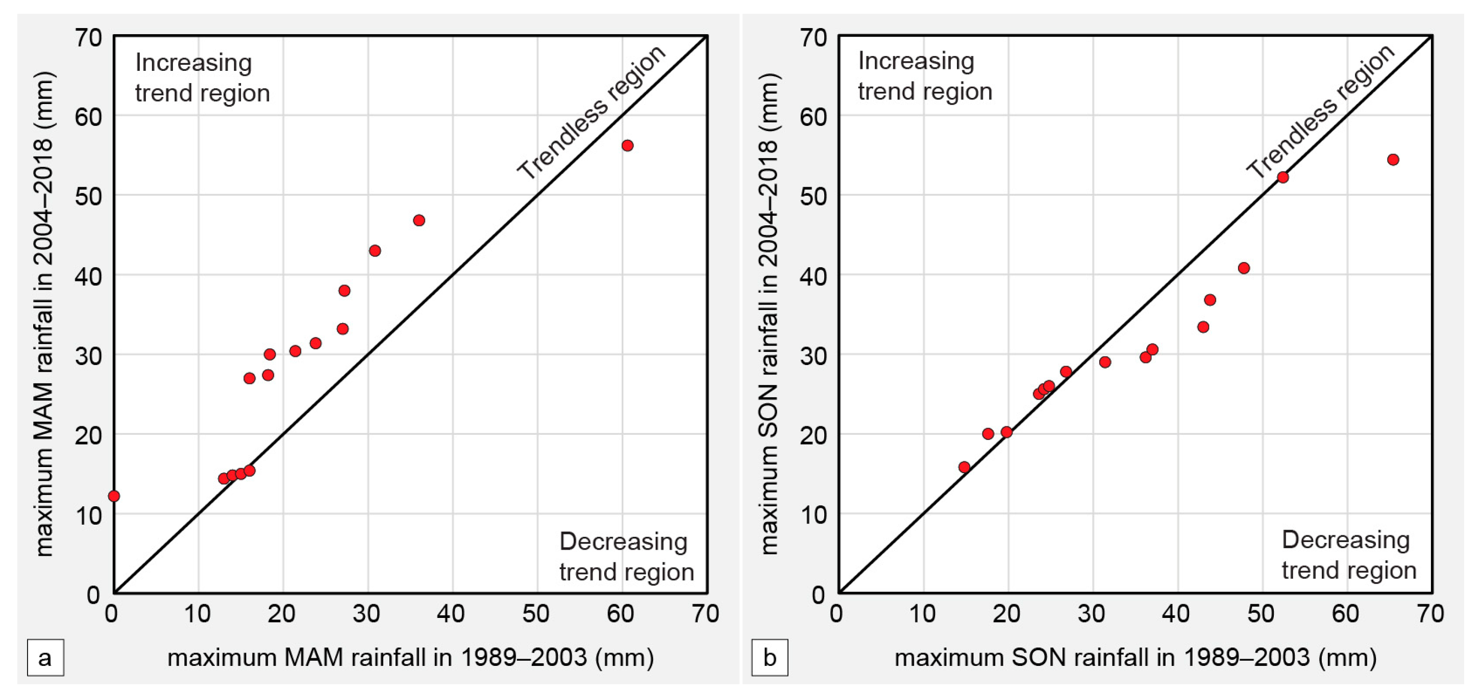
2.2. Climatic Features and Trends
3. Materials and Methods
3.1. DInSAR Analysis
3.2. Geomorphological Analysis
- Inventory of landslide phenomena in Italy (IFFI), available in polygonal shapefile format (https://www.progettoiffi.isprambiente.it/ (accessed on 1 September 2022) and https://idrogeo.isprambiente.it/app/ (accessed on 1 September 2022)).
- Geological map of Italy, available as a WMS service on the Italian National Geoportal (http://wms.pcn.minambiente.it/ogc?map=/ms_ogc/WMS_v1.3/Vettor-ali/Carta_geolitologica.map; accessed on 1 September 2022).
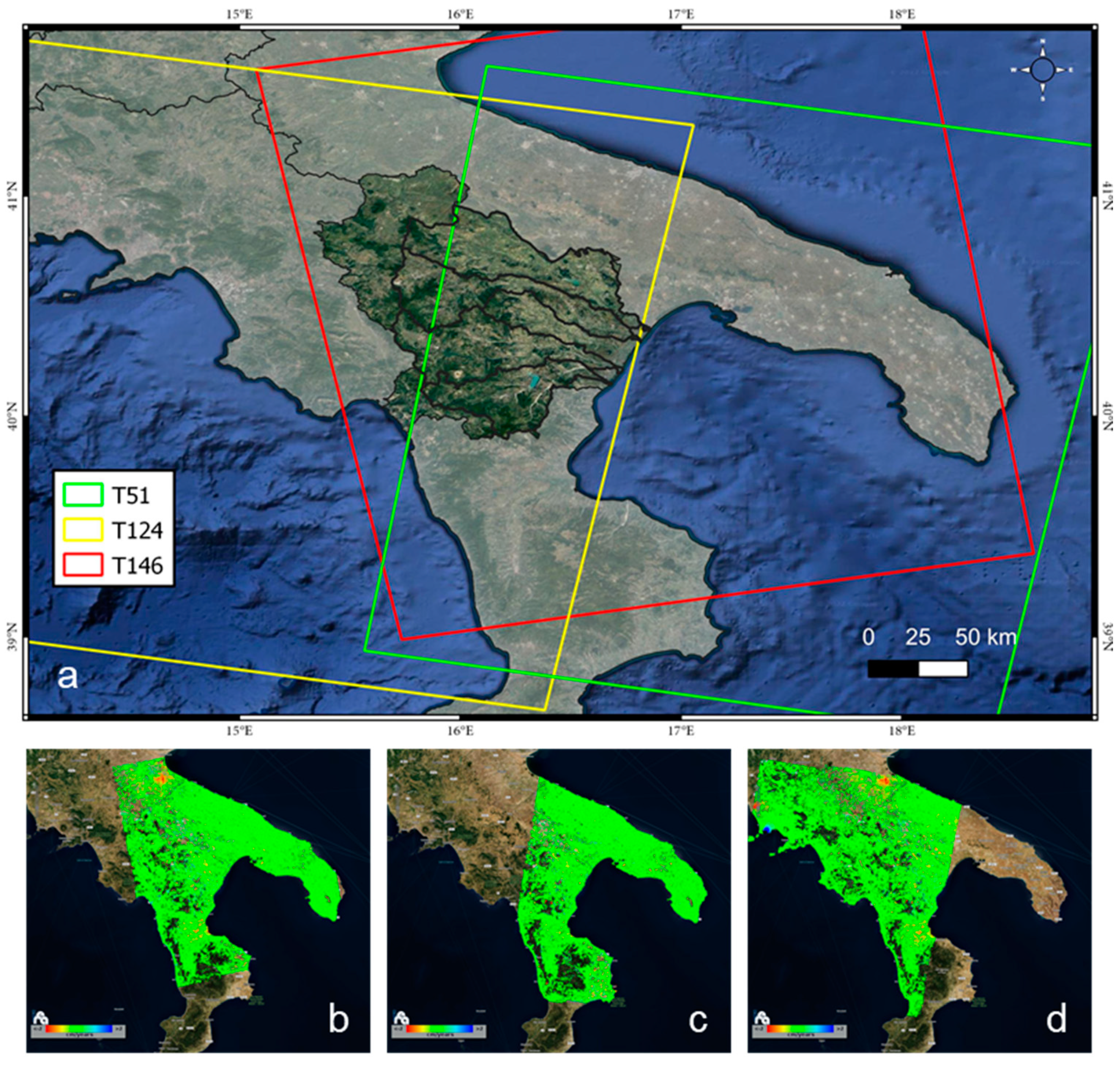
- Maps of ground deformation and associated “time series” prepared for the OT4CLIMA project from Sentinel-1 images in ascending and descending orbits, for the time period 2015–2020, in shapefile format (point geometry).
- Map of the rain gauges and the daily rainfall measurements (provided by the Decentralized Functional Center of the Basilicata Region civil protection, http://www.centrofunzionalebasilicata.it/it/; accessed on 1 September 2022).
- Literature and technical documentation and consultation of local online newspapers related to landslide activity in the Basilicata region.
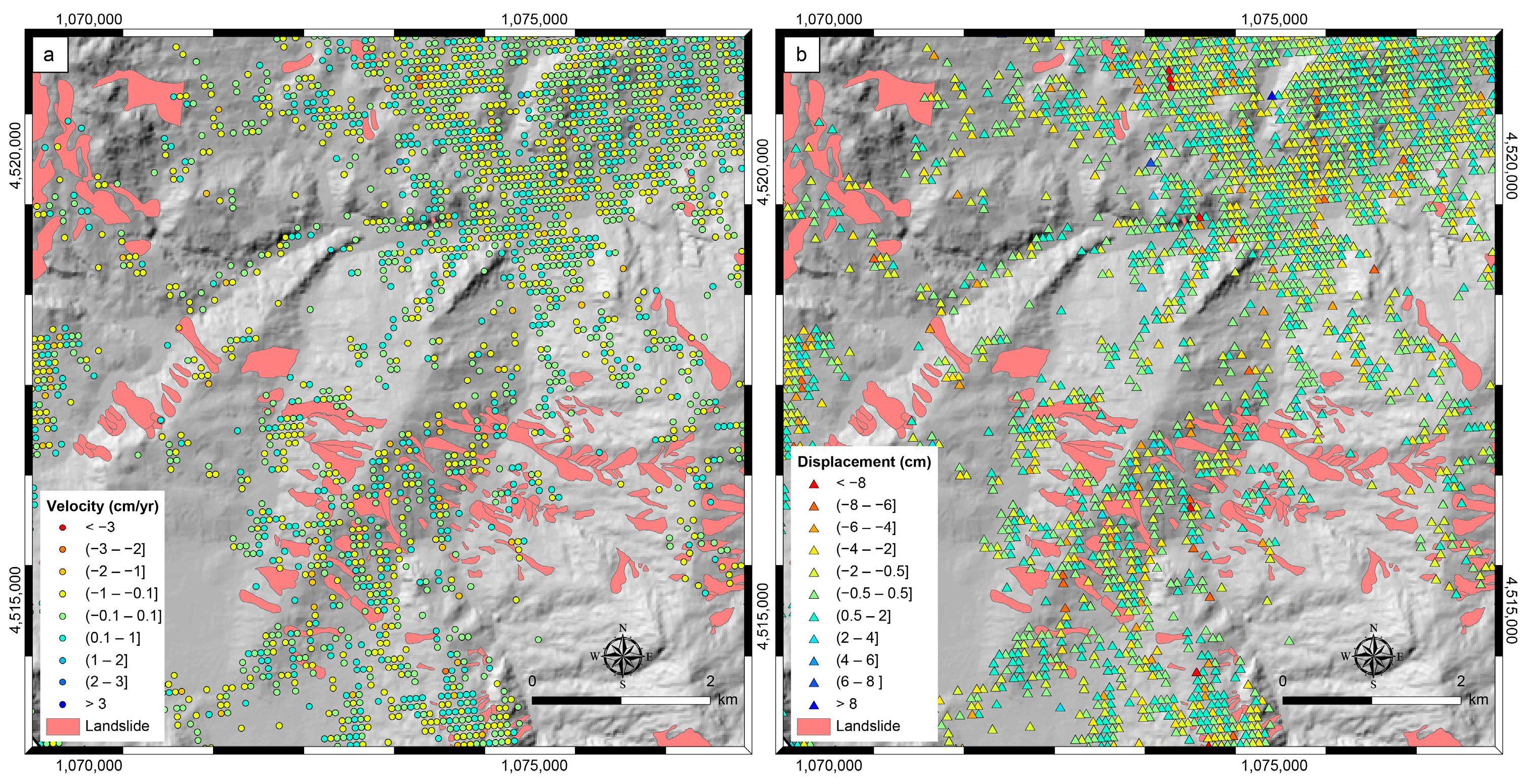
- In the GIS environment, the velocity maps were overlaid on the IFFI landslide shapefile, the geological map and the map of the rain gauges by keeping as background the Google Earth and/or Bing satellite image.
- Through a GIS intersection, the pixels on the velocity maps that fell within a circular buffer of a 10 km radius from the rain gauges were selected. This radius can be considered as a probable influence range of the rain on landslides, it is also in accordance with several works dealing with the reconstruction of rain-gauge-based rainfall events able to trigger landslides in Italy (e.g., [57] and references therein)
- The selected pixels were classified based on the average velocity of deformation (Figure 5a) over the five years of observation (2015–2020) and the cumulative measure of deformation at the last measurement date (Figure 5b). In the average velocity classification, the pixels characterized by a velocity between −0.1 and 0.1 cm/year were considered “stationary” and excluded from the further analyses.
- The pixels with analogous increasing or decreasing trends located in or around landslide areas were put in clusters.
- Information on landslide activities from the scientific literature, online newspapers and technical documents were analyzed to select the landslides characterized by the same state of activity.
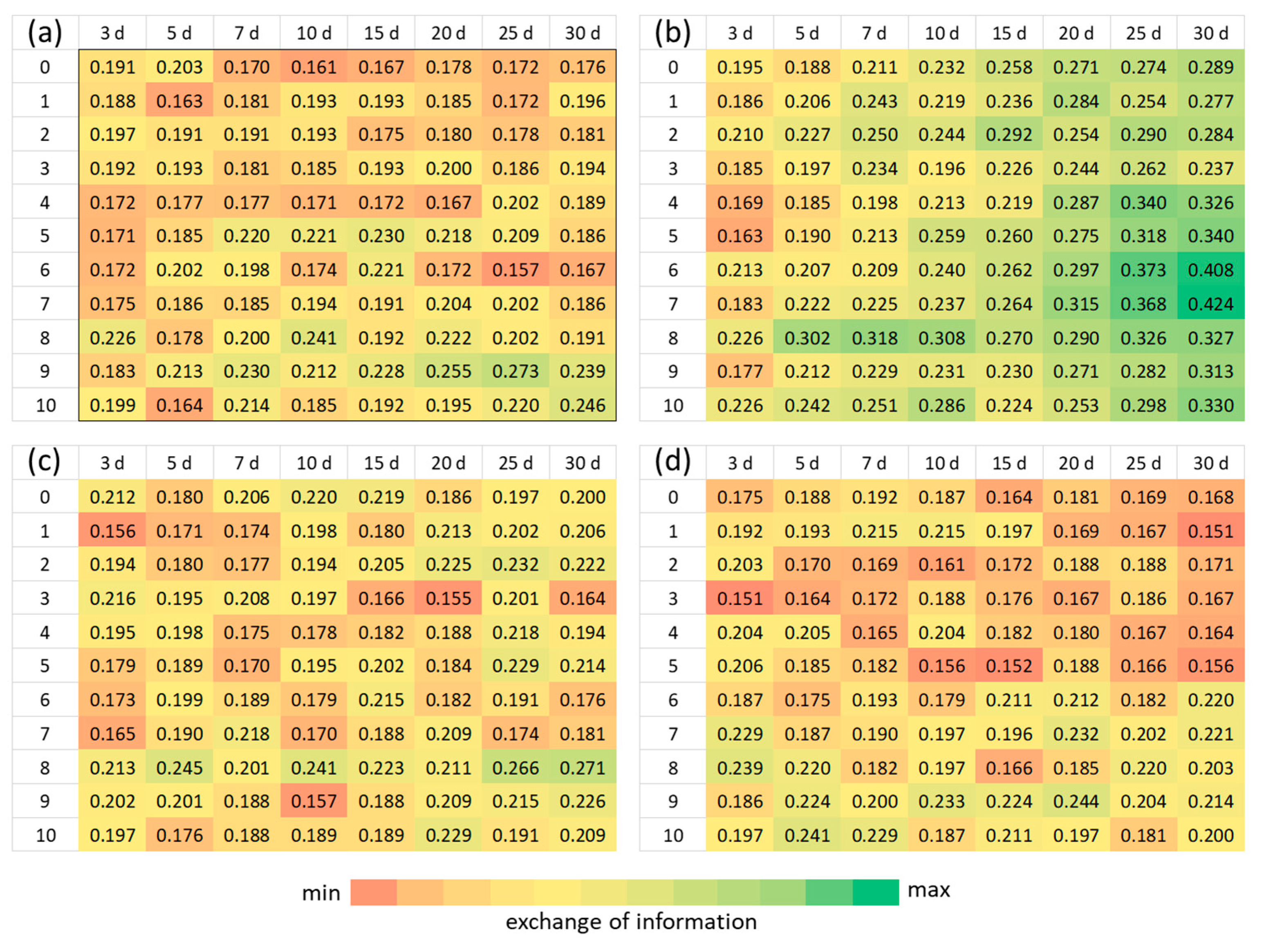
3.3. Statistical Analysis
4. Results
5. Discussion
6. Conclusions
Author Contributions
Funding
Data Availability Statement
Acknowledgments
Conflicts of Interest
References
- Sidle, R.C.; Ochiai, H. Landslides Processes, Prediction, and Land Use; Water Resources Monograph; American Geophysical Union: Washington, DC, WA, USA, 2006; Volume 18, ISBN 978-0-87590-322-4. [Google Scholar]
- IPCC. Climate Change 2014: Synthesis Report. Contribution of Working Groups I, II and III to the Fifth Assessment Report of the Intergovernmental Panel on Climate Change; IPCC: Geneva, Switzerland, 2014; p. 151. ISBN 978-92-9169-143-2.
- IPCC. Climate Change 2022: Impacts, Adaptation and Vulnerability. Contribution of Working Group II to the Sixth Assessment Report of the Intergovernmental Panel on Climate Change; Cambridge University Press: Cambridge, UK; New York, NY, USA, 2022; p. 3056.
- Gariano, S.L.; Guzzetti, F. Landslides in a Changing Climate. Earth-Sci. Rev. 2016, 162, 227–252. [Google Scholar] [CrossRef]
- Gariano, S.L.; Guzzetti, F. Mass-Movements and Climate Change. In Treatise on Geomorphology; Elsevier: Amsterdam, The Netherlands, 2022; pp. 546–558. ISBN 978-0-12-818235-2. [Google Scholar]
- Massonnet, D.; Feigl, K.L. Radar Interferometry and Its Application to Changes in the Earth’s Surface. Rev. Geophys. 1998, 36, 441–500. [Google Scholar] [CrossRef]
- Franceschetti, G.; Lanari, R. Synthetic Aperture Radar Processing; CRC Press: Boca Raton, FL, USA, 1999; ISBN 978-0-8493-7899-7. [Google Scholar]
- Talledo, D.A.; Miano, A.; Bonano, M.; Di Carlo, F.; Lanari, R.; Manunta, M.; Meda, A.; Mele, A.; Prota, A.; Saetta, A.; et al. Satellite Radar Interferometry: Potential and Limitations for Structural Assessment and Monitoring. J. Build. Eng. 2022, 46, 103756. [Google Scholar] [CrossRef]
- Monterroso, F.; Bonano, M.; Luca, C.D.; Lanari, R.; Manunta, M.; Manzo, M.; Onorato, G.; Zinno, I.; Casu, F. A Global Archive of Coseismic DInSAR Products Obtained through Unsupervised Sentinel-1 Data Processing. Remote Sens. 2020, 12, 3189. [Google Scholar] [CrossRef]
- Schreier, G. Opportunities by the Copernicus Program for Archaeological Research and World Heritage Site Conservation. In Remote Sensing for Archaeology and Cultural Landscapes: Best Practices and Perspectives across Europe and the Middle East; Hadjimitsis, D.G., Themistocleous, K., Cuca, B., Agapiou, A., Lysandrou, V., Lasaponara, R., Masini, N., Schreier, G., Eds.; Springer Remote Sensing/Photogrammetry; Springer International Publishing: Cham, Switzerland, 2020; pp. 3–18. ISBN 978-3-030-10979-0. [Google Scholar]
- Solari, L.; Del Soldato, M.; Bianchini, S.; Ciampalini, A.; Ezquerro, P.; Montalti, R.; Raspini, F.; Moretti, S. From ERS 1/2 to Sentinel-1: Subsidence Monitoring in Italy in the Last Two Decades. Front. Earth Sci. 2018, 6, 149. [Google Scholar] [CrossRef]
- Tang, W.; Motagh, M.; Zhan, W. Monitoring Active Open-Pit Mine Stability in the Rhenish Coalfields of Germany Using a Coherence-Based SBAS Method. Int. J. Appl. Earth Obs. Geoinf. 2020, 93, 102217. [Google Scholar] [CrossRef]
- Solari, L.; Del Soldato, M.; Raspini, F.; Barra, A.; Bianchini, S.; Confuorto, P.; Casagli, N.; Crosetto, M. Review of Satellite Interferometry for Landslide Detection in Italy. Remote Sens. 2020, 12, 1351. [Google Scholar] [CrossRef]
- Moretto, S.; Bozzano, F.; Mazzanti, P. The Role of Satellite InSAR for Landslide Forecasting: Limitations and Openings. Remote Sens. 2021, 13, 3735. [Google Scholar] [CrossRef]
- Wasowski, J.; Bovenga, F. Investigating Landslides and Unstable Slopes with Satellite Multi Temporal Interferometry: Current Issues and Future Perspectives. Eng. Geol. 2014, 174, 103–138. [Google Scholar] [CrossRef]
- Mondini, A.C.; Guzzetti, F.; Chang, K.-T.; Monserrat, O.; Martha, T.R.; Manconi, A. Landslide Failures Detection and Mapping Using Synthetic Aperture Radar: Past, Present and Future. Earth-Sci. Rev. 2021, 216, 103574. [Google Scholar] [CrossRef]
- Confuorto, P.; Di Martire, D.; Centolanza, G.; Iglesias, R.; Mallorqui, J.J.; Novellino, A.; Plank, S.; Ramondini, M.; Thuro, K.; Calcaterra, D. Post-Failure Evolution Analysis of a Rainfall-Triggered Landslide by Multi-Temporal Interferometry SAR Approaches Integrated with Geotechnical Analysis. Remote Sens. Environ. 2017, 188, 51–72. [Google Scholar] [CrossRef]
- Pappalardo, G.; Mineo, S.; Angrisani, A.C.; Di Martire, D.; Calcaterra, D. Combining Field Data with Infrared Thermography and DInSAR Surveys to Evaluate the Activity of Landslides: The Case Study of Randazzo Landslide (NE Sicily). Landslides 2018, 15, 2173–2193. [Google Scholar] [CrossRef]
- García-Davalillo, J.C.; Herrera, G.; Notti, D.; Strozzi, T.; Álvarez-Fernández, I. DInSAR Analysis of ALOS PALSAR Images for the Assessment of Very Slow Landslides: The Tena Valley Case Study. Landslides 2014, 11, 225–246. [Google Scholar] [CrossRef]
- Pourkhosravani, M.; Mehrabi, A.; Pirasteh, S.; Derakhshani, R. Monitoring of Maskun Landslide and Determining Its Quantitative Relationship to Different Climatic Conditions Using D-InSAR and PSI Techniques. Geomat. Nat. Hazards Risk 2022, 13, 1134–1153. [Google Scholar] [CrossRef]
- Wasowski, J.; Pisano, L. Long-Term InSAR, Borehole Inclinometer, and Rainfall Records Provide Insight into the Mechanism and Activity Patterns of an Extremely Slow Urbanized Landslide. Landslides 2020, 17, 445–457. [Google Scholar] [CrossRef]
- Bordoni, M.; Bonì, R.; Colombo, A.; Lanteri, L.; Meisina, C. A Methodology for Ground Motion Area Detection (GMA-D) Using A-DInSAR Time Series in Landslide Investigations. CATENA 2018, 163, 89–110. [Google Scholar] [CrossRef]
- Vassallo, R.; Calcaterra, S.; D’Agostino, N.; De Rosa, J.; Di Maio, C.; Gambino, P. Long-Term Displacement Monitoring of Slow Earthflows by Inclinometers and GPS, and Wide Area Surveillance by COSMO-SkyMed Data. Geosciences 2020, 10, 171. [Google Scholar] [CrossRef]
- Carlà, T.; Raspini, F.; Intrieri, E.; Casagli, N. A Simple Method to Help Determine Landslide Susceptibility from Spaceborne InSAR Data: The Montescaglioso Case Study. Environ. Earth Sci. 2016, 75, 1492. [Google Scholar] [CrossRef]
- Ardizzone, F.; Rossi, M.; Calò, F.; Paglia, L.; Manunta, M.; Mondini, A.C.; Zeni, G.; Reichenbach, P.; Lanari, R.; Guzzetti, F. Preliminary Analysis of a Correlation between Ground Deformations and Rainfall: The Ivancich Landslide, Central Italy. In Proceedings of the SAR Image Analysis, Modeling, and Techniques XI, Prague, Czech Republic, 26 October 2011; Volume 8179, pp. 167–175. [Google Scholar]
- Herrera, G.; Gutiérrez, F.; García-Davalillo, J.C.; Guerrero, J.; Notti, D.; Galve, J.P.; Fernández-Merodo, J.A.; Cooksley, G. Multi-Sensor Advanced DInSAR Monitoring of Very Slow Landslides: The Tena Valley Case Study (Central Spanish Pyrenees). Remote Sens. Environ. 2013, 128, 31–43. [Google Scholar] [CrossRef]
- Reyes-Carmona, C.; Barra, A.; Galve, J.P.; Monserrat, O.; Pérez-Peña, J.V.; Mateos, R.M.; Notti, D.; Ruano, P.; Millares, A.; López-Vinielles, J.; et al. Sentinel-1 DInSAR for Monitoring Active Landslides in Critical Infrastructures: The Case of the Rules Reservoir (Southern Spain). Remote Sens. 2020, 12, 809. [Google Scholar] [CrossRef]
- Fobert, M.-A.; Singhroy, V.; Spray, J.G. InSAR Monitoring of Landslide Activity in Dominica. Remote Sens. 2021, 13, 815. [Google Scholar] [CrossRef]
- Muñoz-Torrero Manchado, A.; Allen, S.; Ballesteros-Cánovas, J.A.; Dhakal, A.; Dhital, M.R.; Stoffel, M. Three Decades of Landslide Activity in Western Nepal: New Insights into Trends and Climate Drivers. Landslides 2021, 18, 2001–2015. [Google Scholar] [CrossRef]
- Doglioni, C. A Proposal for the Kinematic Modelling of W-Dipping Subductions-Possible Applications to the Tyrrhenian-Apennines System. Terra Nova 1991, 3, 423–434. [Google Scholar] [CrossRef]
- Giano, S.I.; Gioia, D.; Schiattarella, M. Morphotectonic Evolution of Connected Intermontane Basins from the Southern Apennines, Italy: The Legacy of the Pre-Existing Structurally Controlled Landscape. Rend. Lincei 2014, 25, 241–252. [Google Scholar] [CrossRef]
- Bentivenga, M.; Palladino, G.; Prosser, G.; Guglielmi, P.; Geremia, F.; Laviano, A. A Geological Itinerary Through the Southern Apennine Thrust Belt (Basilicata—Southern Italy). Geoheritage 2017, 9, 1–17. [Google Scholar] [CrossRef]
- Lazzari, M.; Gioia, D. Regional-Scale Landslide Inventory, Central-Western Sector of the Basilicata Region (Southern Apennines, Italy). J. Maps 2016, 12, 852–859. [Google Scholar] [CrossRef]
- Bucci, F.; Santangelo, M.; Fiorucci, F.; Ardizzone, F.; Giordan, D.; Cignetti, M.; Notti, D.; Allasia, P.; Godone, D.; Lagomarsino, D.; et al. Geomorphologic Landslide Inventory by Air Photo Interpretation of the High Agri Valley (Southern Italy). J. Maps 2021, 17, 376–388. [Google Scholar] [CrossRef]
- Lazzari, M.; Gioia, D.; Anzidei, B. Landslide Inventory of the Basilicata Region (Southern Italy). J. Maps 2018, 14, 348–356. [Google Scholar] [CrossRef]
- Bentivenga, M.; Bellanova, J.; Calamita, G.; Capece, A.; Cavalcante, F.; Gueguen, E.; Guglielmi, P.; Murgante, B.; Palladino, G.; Perrone, A.; et al. Geomorphological and Geophysical Surveys with InSAR Analysis Applied to the Picerno Earth Flow (Southern Apennines, Italy). Landslides 2021, 18, 471–483. [Google Scholar] [CrossRef]
- Lazzari, M.; Piccarreta, M.; Ray, R.L.; Manfreda, S. Modeling Antecedent Soil Moisture to Constrain Rainfall Thresholds for Shallow Landslides Occurrence. In Landslides-Investigation and Monitoring; Ray, R., Lazzari, M., Eds.; IntechOpen: London, UK, 2020; ISBN 978-1-78985-823-5. [Google Scholar]
- Perrone, A. Lessons Learned by 10 Years of Geophysical Measurements with Civil Protection in Basilicata (Italy) Landslide Areas. Landslides 2021, 18, 1499–1508. [Google Scholar] [CrossRef]
- Lazzari, M. Note Illustrative Della Carta Inventario Delle Frane Della Basilicata Centroccidentale; Zaccara: Lagonegro, Italy, 2011; p. 136. [Google Scholar]
- Guida, D. Iaccarino Fasi evolutive delle frane tipo colata nell’alta valle del F. Basento (Potenza). Studi Trentini Di Sci. Nat. Acta Geol. 1991, 68, 127–152. [Google Scholar]
- Urciuoli, G.; Comegna, L.; Di Maio, C.; Picarelli, L. The Basento Valley: A Natural Laboratory to Understand the Mechanics of Earthflows. Riv. Ital. Geotec. 2016, 1, 71–90. [Google Scholar]
- Peel, M.C.; Finlayson, B.L.; McMahon, T.A. Updated World Map of the Köppen-Geiger Climate Classification. Hydrol. Earth Syst. Sci. 2007, 11, 1633–1644. [Google Scholar] [CrossRef]
- Piccarreta, M.; Pasini, A.; Capolongo, D.; Lazzari, M. Changes in Daily Precipitation Extremes in the Mediterranean from 1951 to 2010: The Basilicata Region, Southern Italy. Int. J. Climatol. 2013, 33, 3229–3248. [Google Scholar] [CrossRef]
- Şen, Z. Innovative Trend Analysis Methodology. J. Hydrol. Eng. 2012, 17, 1042–1046. [Google Scholar] [CrossRef]
- Şen, Z. Trend Identification Simulation and Application. J. Hydrol. Eng. 2014, 19, 635–642. [Google Scholar] [CrossRef]
- Şen, Z. Innovative Trend Significance Test and Applications. Theor. Appl. Climatol. 2017, 127, 939–947. [Google Scholar] [CrossRef]
- Caloiero, T.; Coscarelli, R.; Ferrari, E. Application of the Innovative Trend Analysis Method for the Trend Analysis of Rainfall Anomalies in Southern Italy. Water Resour. Manag. 2018, 32, 4971–4983. [Google Scholar] [CrossRef]
- Berardino, P.; Fornaro, G.; Lanari, R.; Sansosti, E. A New Algorithm for Surface Deformation Monitoring Based on Small Baseline Differential SAR Interferograms. IEEE Trans. Geosci. Remote Sens. 2002, 40, 2375–2383. [Google Scholar] [CrossRef]
- Casu, F.; Elefante, S.; Imperatore, P.; Zinno, I.; Manunta, M.; De Luca, C.; Lanari, R. SBAS-DInSAR Parallel Processing for Deformation Time-Series Computation. IEEE J. Sel. Top. Appl. Earth Obs. Remote Sens. 2014, 7, 3285–3296. [Google Scholar] [CrossRef]
- Manunta, M.; De Luca, C.; Zinno, I.; Casu, F.; Manzo, M.; Bonano, M.; Fusco, A.; Pepe, A.; Onorato, G.; Berardino, P.; et al. The Parallel SBAS Approach for Sentinel-1 Interferometric Wide Swath Deformation Time-Series Generation: Algorithm Description and Products Quality Assessment. IEEE Trans. Geosci. Remote Sens. 2019, 57, 6259–6281. [Google Scholar] [CrossRef]
- Lanari, R.; Bonano, M.; Casu, F.; Luca, C.D.; Manunta, M.; Manzo, M.; Onorato, G.; Zinno, I. Automatic Generation of Sentinel-1 Continental Scale DInSAR Deformation Time Series through an Extended P-SBAS Processing Pipeline in a Cloud Computing Environment. Remote Sens. 2020, 12, 2961. [Google Scholar] [CrossRef]
- Zinno, I.; Bonano, M.; Buonanno, S.; Casu, F.; De Luca, C.; Manunta, M.; Manzo, M.; Lanari, R. National Scale Surface Deformation Time Series Generation through Advanced DInSAR Processing of Sentinel-1 Data within a Cloud Computing Environment. IEEE Trans. Big Data 2020, 6, 558–571. [Google Scholar] [CrossRef]
- Blewitt, G.; Hammond, W.C.; Kreemer, C. Harnessing the GPS Data Explosion for Interdisciplinary Science. Eos 2018, 99, 485. [Google Scholar] [CrossRef]
- Sansosti, E.; Berardino, P.; Manunta, M.; Serafino, F.; Fornaro, G. Geometrical SAR Image Registration. IEEE Trans. Geosci. Remote Sens. 2006, 44, 2861–2870. [Google Scholar] [CrossRef]
- Pepe, A.; Yang, Y.; Manzo, M.; Lanari, R. Improved EMCF-SBAS Processing Chain Based on Advanced Techniques for the Noise-Filtering and Selection of Small Baseline Multi-Look DInSAR Interferograms. IEEE Trans. Geosci. Remote Sens. 2015, 53, 4394–4417. [Google Scholar] [CrossRef]
- Pepe, A.; Lanari, R. On the Extension of the Minimum Cost Flow Algorithm for Phase Unwrapping of Multitemporal Differential SAR Interferograms. IEEE Trans. Geosci. Remote Sens. 2006, 44, 2374–2383. [Google Scholar] [CrossRef]
- Peruccacci, S.; Brunetti, M.T.; Gariano, S.L.; Melillo, M.; Rossi, M.; Guzzetti, F. Rainfall Thresholds for Possible Landslide Occurrence in Italy. Geomorphology 2017, 290, 39–57. [Google Scholar] [CrossRef]
- Kendall, M.G. A New Measure of Rank Correlation. Biometrika 1938, 30, 81–93. [Google Scholar] [CrossRef]
- Reshef, D.N.; Reshef, Y.A.; Finucane, H.K.; Grossman, S.R.; McVean, G.; Turnbaugh, P.J.; Lander, E.S.; Mitzenmacher, M.; Sabeti, P.C. Detecting Novel Associations in Large Data Sets. Science 2011, 334, 1518–1524. [Google Scholar] [CrossRef]
- Kendall, M.G. The Treatment of Ties in Ranking Problems. Biometrika 1945, 33, 239–251. [Google Scholar] [CrossRef] [PubMed]
- Brillouin, L. Science and Information Theory, 2nd ed.; Dover Publications, Inc.: Mineola, NY, USA, 2013; ISBN 978-0-486-49755-6. [Google Scholar]
- Zhang, Y.; Jia, S.; Huang, H.; Qiu, J.; Zhou, C. A Novel Algorithm for the Precise Calculation of the Maximal Information Coefficient. Sci. Rep. 2015, 4, 6662. [Google Scholar] [CrossRef] [PubMed]
- Festa, D.; Bonano, M.; Casagli, N.; Confuorto, P.; De Luca, C.; Del Soldato, M.; Lanari, R.; Lu, P.; Manunta, M.; Manzo, M.; et al. Nation-Wide Mapping and Classification of Ground Deformation Phenomena through the Spatial Clustering of P-SBAS InSAR Measurements: Italy Case Study. ISPRS J. Photogramm. Remote Sens. 2022, 189, 1–22. [Google Scholar] [CrossRef]
- Naudet, V.; Lazzari, M.; Perrone, A.; Loperte, A.; Piscitelli, S.; Lapenna, V. Integrated Geophysical and Geomorphological Approach to Investigate the Snowmelt-Triggered Landslide of Bosco Piccolo Village (Basilicata, Southern Italy). Eng. Geol. 2008, 98, 156–167. [Google Scholar] [CrossRef]
- Borfecchia, F.; De Canio, G.; De Cecco, L.; Giocoli, A.; Grauso, S.; La Porta, L.; Martini, S.; Pollino, M.; Roselli, I.; Zini, A. Mapping the Earthquake-Induced Landslide Hazard around the Main Oil Pipeline Network of the Agri Valley (Basilicata, Southern Italy) by Means of Two GIS-Based Modelling Approaches. Nat. Hazards 2016, 81, 759–777. [Google Scholar] [CrossRef]
- Gizzi, F.T.; Potenza, M.R. The Scientific Landscape of November 23rd, 1980 Irpinia-Basilicata Earthquake: Taking Stock of (Almost) 40 Years of Studies. Geosciences 2020, 10, 482. [Google Scholar] [CrossRef]
- Cedit-Italian Catalogue of Earthquake-Induced Ground Failures-GeoDB. Available online: https://gdb.ceri.uniroma1.it/index.php/view/map/?repository=cedit&project=Cedit (accessed on 8 August 2022).
- Bonì, R.; Bordoni, M.; Vivaldi, V.; Troisi, C.; Tararbra, M.; Lanteri, L.; Zucca, F.; Meisina, C. Assessment of the Sentinel-1 Based Ground Motion Data Feasibility for Large Scale Landslide Monitoring. Landslides 2020, 17, 2287–2299. [Google Scholar] [CrossRef]
- Guo, Z.; Yin, K.; Gui, L.; Liu, Q.; Huang, F.; Wang, T. Regional Rainfall Warning System for Landslides with Creep Deformation in Three Gorges Using a Statistical Black Box Model. Sci. Rep. 2019, 9, 8962. [Google Scholar] [CrossRef]
- Bordoni, M.; Vivaldi, V.; Bonì, R.; Spanò, S.; Tararbra, M.; Lanteri, L.; Parnigoni, M.; Grossi, A.; Figini, S.; Meisina, C. A Methodology for the Analysis of Continuous Time-Series of Automatic Inclinometers for Slow-Moving Landslides Monitoring in Piemonte Region, Northern Italy. Nat. Hazards 2022. [Google Scholar] [CrossRef]


| Station (Basin) | Year | DJF | MAM | JJA | SON | ||||||
|---|---|---|---|---|---|---|---|---|---|---|---|
| Total | Max | Total | Max | Total | Max | Total | Max | Total | Max | ||
| Matera (Bradano) | low | + | = | + | = | + | + | + | = | + | + |
| med | + | = | + | = | + | + | + | = | + | = | |
| high | + | + | + | = | + | + | - | = | + | = | |
| Potenza (Basento) | low | + | - | + | = | = | = | = | - | = | = |
| med | + | + | + | = | + | + | + | + | + | - | |
| high | + | - | + | + | + | = | + | - | + | - | |
| San Nicola (Basento) | low | + | + | + | + | + | + | + | + | + | + |
| med | + | + | + | = | + | + | + | + | + | - | |
| high | + | + | + | + | + | + | + | + | + | = | |
| Tramutola (Agri) | low | + | + | + | + | + | + | + | + | + | - |
| med | + | + | + | + | + | + | + | + | = | - | |
| high | + | - | + | = | = | = | = | + | - | - | |
Disclaimer/Publisher’s Note: The statements, opinions and data contained in all publications are solely those of the individual author(s) and contributor(s) and not of MDPI and/or the editor(s). MDPI and/or the editor(s) disclaim responsibility for any injury to people or property resulting from any ideas, methods, instructions or products referred to in the content. |
© 2023 by the authors. Licensee MDPI, Basel, Switzerland. This article is an open access article distributed under the terms and conditions of the Creative Commons Attribution (CC BY) license (https://creativecommons.org/licenses/by/4.0/).
Share and Cite
Ardizzone, F.; Gariano, S.L.; Volpe, E.; Antronico, L.; Coscarelli, R.; Manunta, M.; Mondini, A.C. A Procedure for the Quantitative Comparison of Rainfall and DInSAR-Based Surface Displacement Time Series in Slow-Moving Landslides: A Case Study in Southern Italy. Remote Sens. 2023, 15, 320. https://doi.org/10.3390/rs15020320
Ardizzone F, Gariano SL, Volpe E, Antronico L, Coscarelli R, Manunta M, Mondini AC. A Procedure for the Quantitative Comparison of Rainfall and DInSAR-Based Surface Displacement Time Series in Slow-Moving Landslides: A Case Study in Southern Italy. Remote Sensing. 2023; 15(2):320. https://doi.org/10.3390/rs15020320
Chicago/Turabian StyleArdizzone, Francesca, Stefano Luigi Gariano, Evelina Volpe, Loredana Antronico, Roberto Coscarelli, Michele Manunta, and Alessandro Cesare Mondini. 2023. "A Procedure for the Quantitative Comparison of Rainfall and DInSAR-Based Surface Displacement Time Series in Slow-Moving Landslides: A Case Study in Southern Italy" Remote Sensing 15, no. 2: 320. https://doi.org/10.3390/rs15020320
APA StyleArdizzone, F., Gariano, S. L., Volpe, E., Antronico, L., Coscarelli, R., Manunta, M., & Mondini, A. C. (2023). A Procedure for the Quantitative Comparison of Rainfall and DInSAR-Based Surface Displacement Time Series in Slow-Moving Landslides: A Case Study in Southern Italy. Remote Sensing, 15(2), 320. https://doi.org/10.3390/rs15020320