
YOLOLens: A Deep Learning Model Based on Super-Resolution to Enhance the Crater Detection of the Planetary Surfaces

 , ,
, ,  , and
, and
Abstract
1. Introduction
2. Background
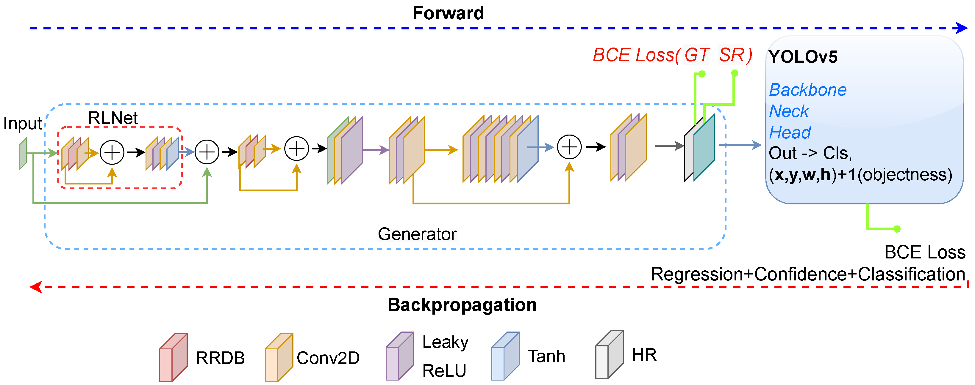
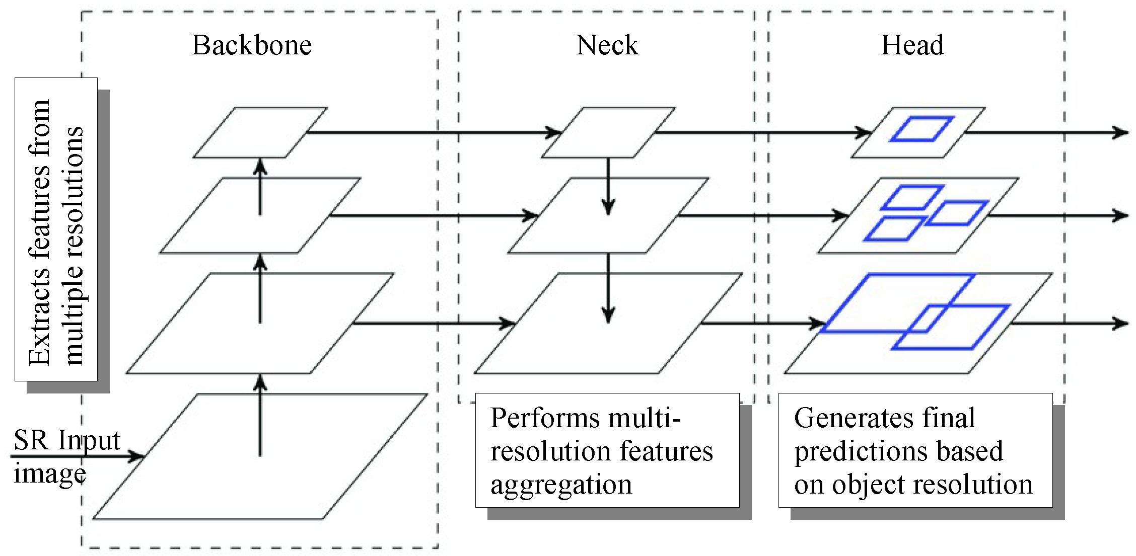
3. Methodology
4. Dataset
Data Preprocessing Details and Craters Extraction
- Convert global mosaic tiff to a png image.
- Read Robbins catalogue and discard all craters largest than the window selected.
- Select N random tiles and reproject them to the orthographic coordinates system.
- (a)
- Cut off all tiles outside the selected window (avoid no data regions)
- (b)
- Avoid all tiles with too dilatation
- (c)
- Discard all tiles with no Ground-Truth correspondence from the catalogue selected
- (d)
- Convert from Lon/Lat system to Pixel reference and normalize in [0–1] values.
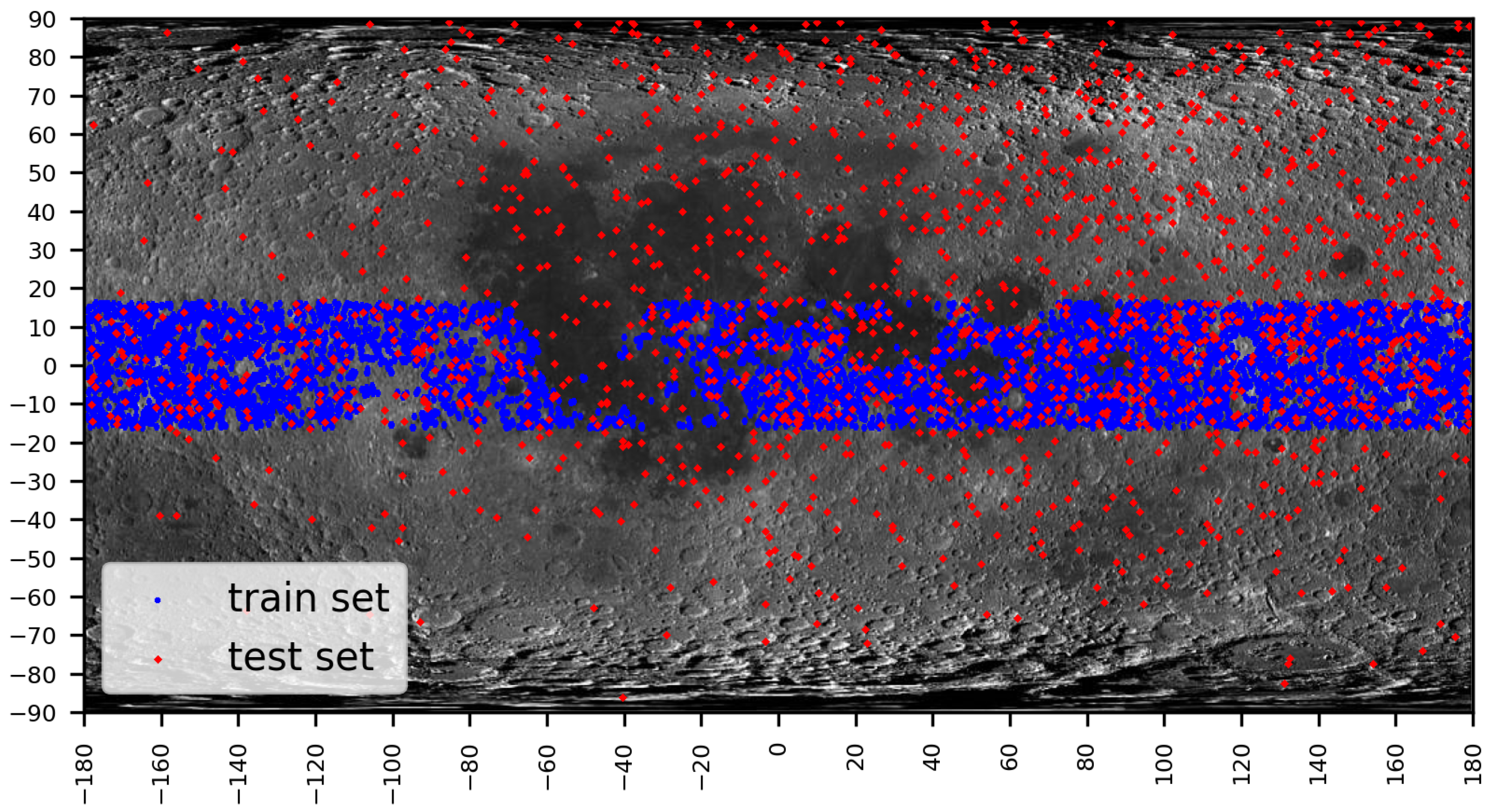
- Split into train/eval in a ratio of 80:20 and save the tiles obtained.
- Convert all information into a YOLO format dataset.
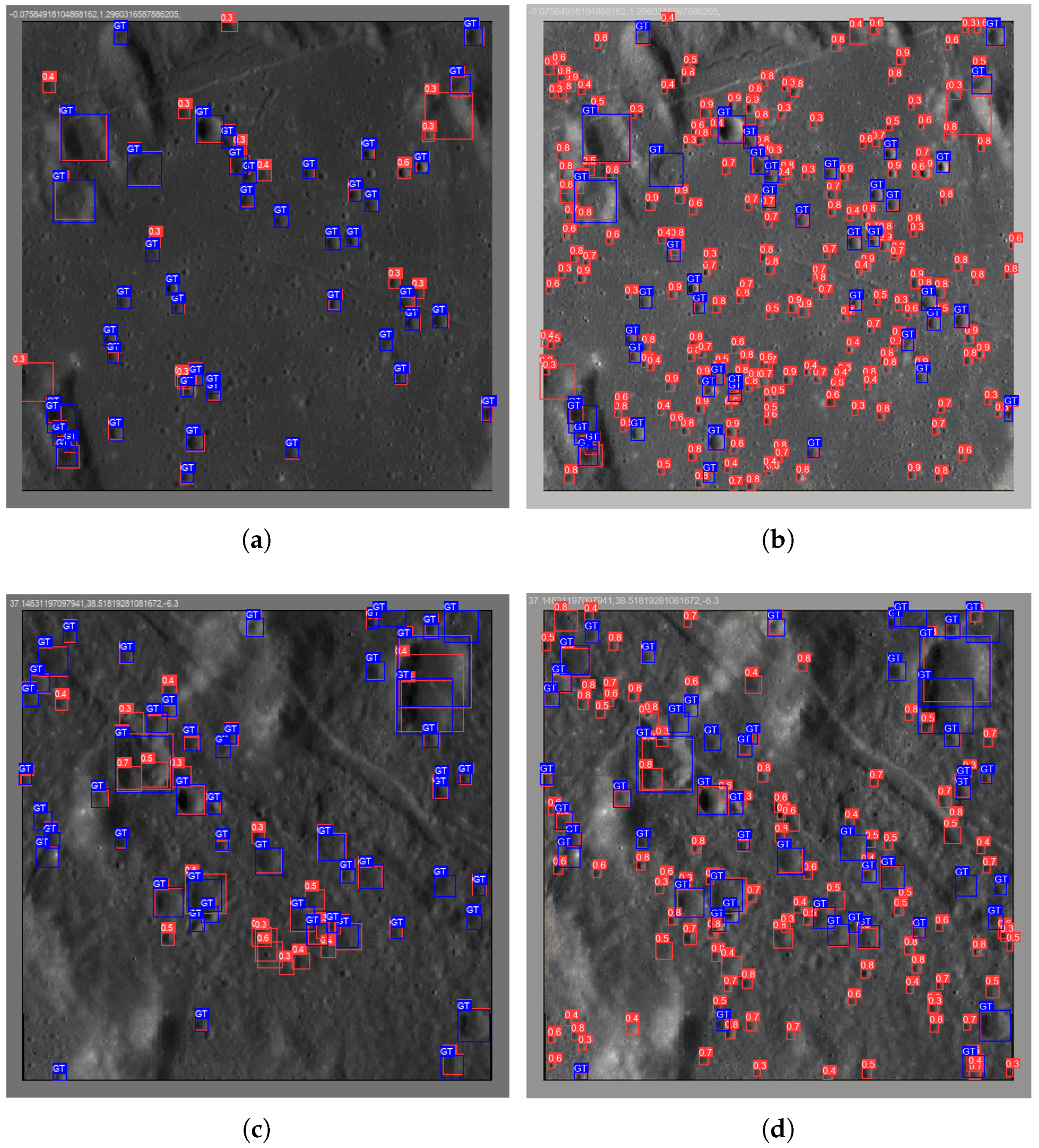
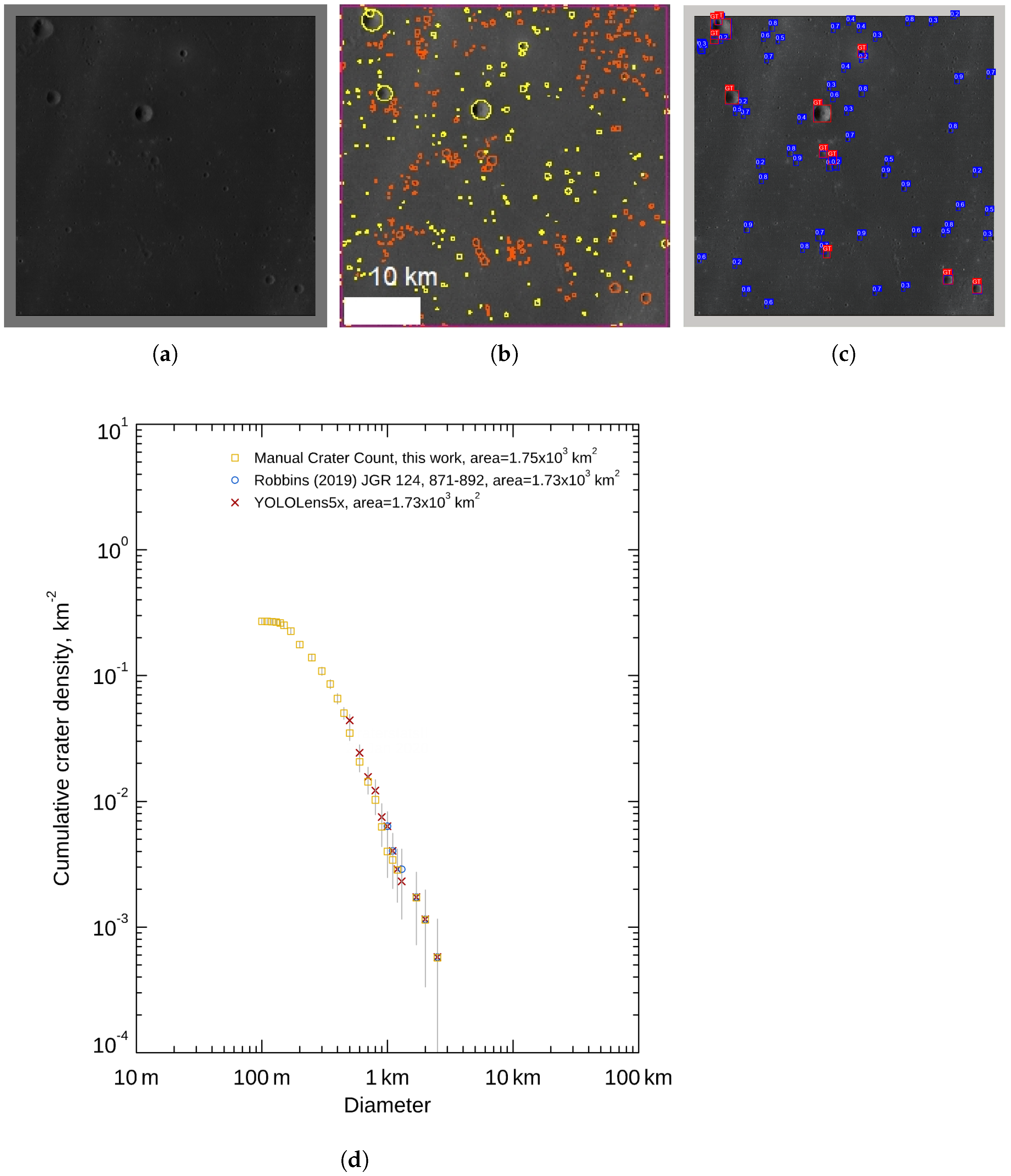
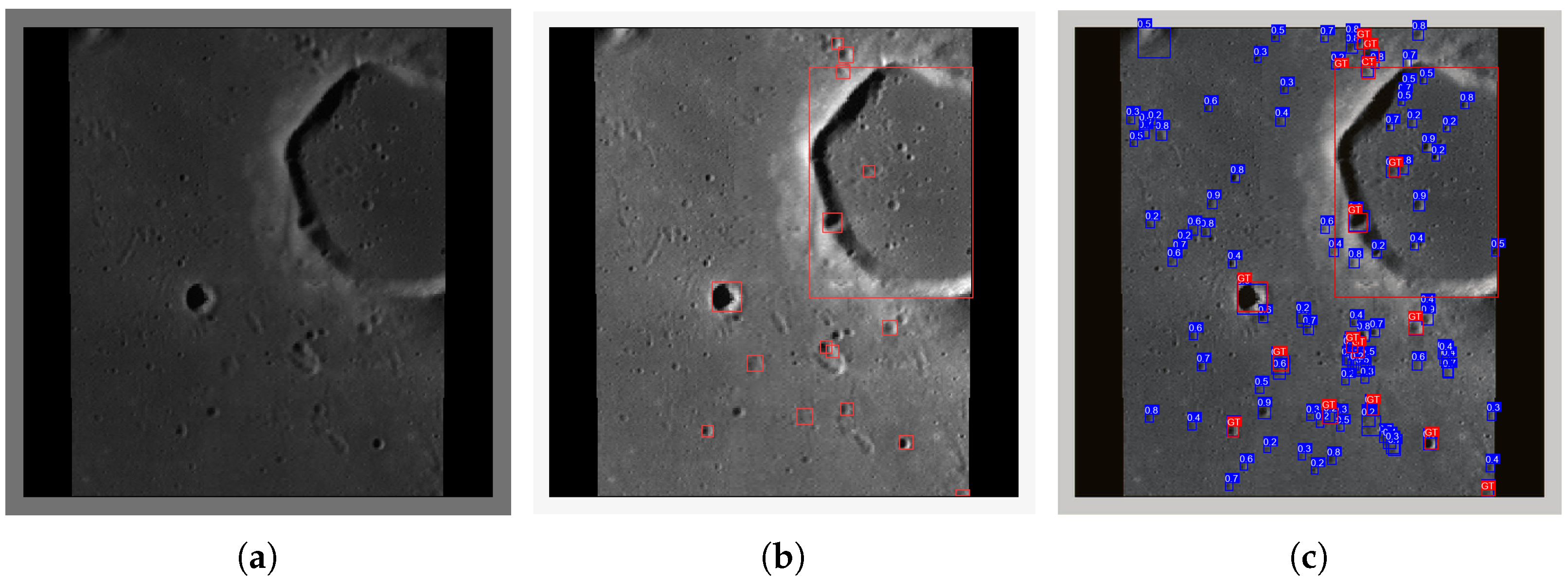
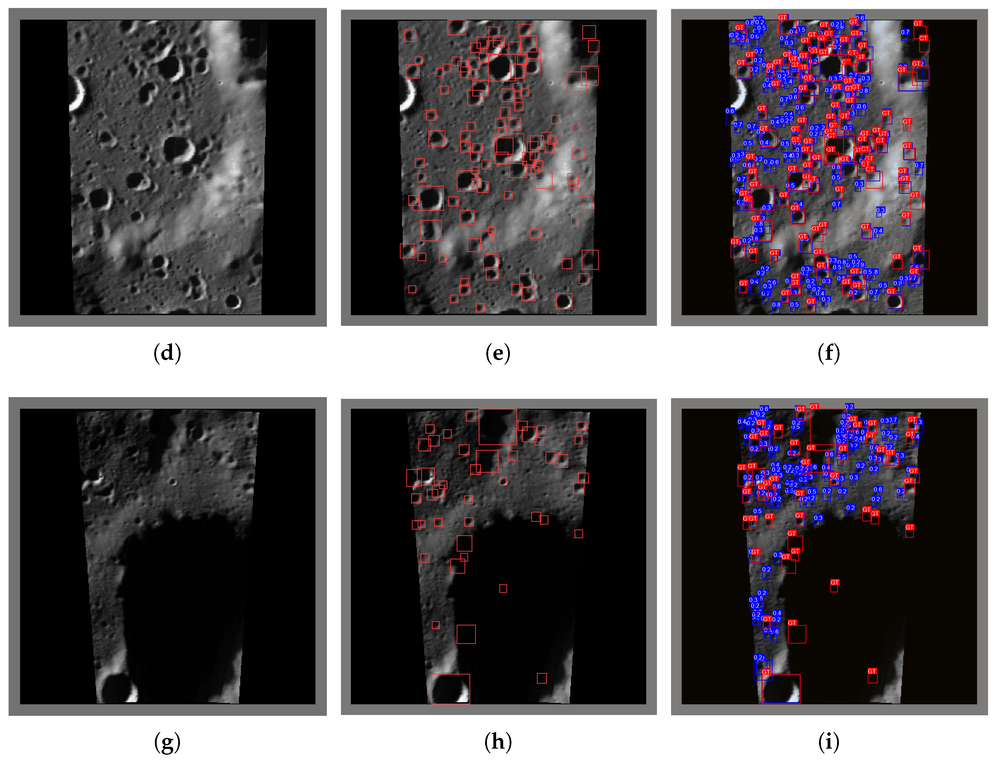
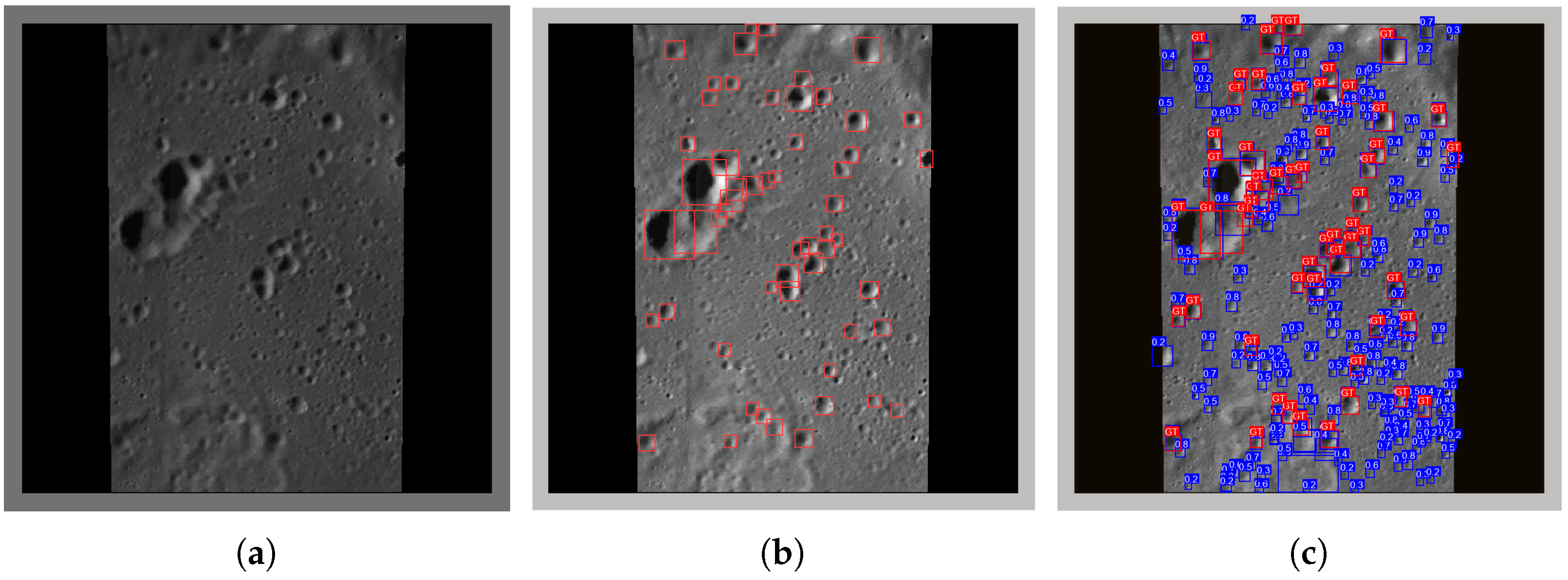
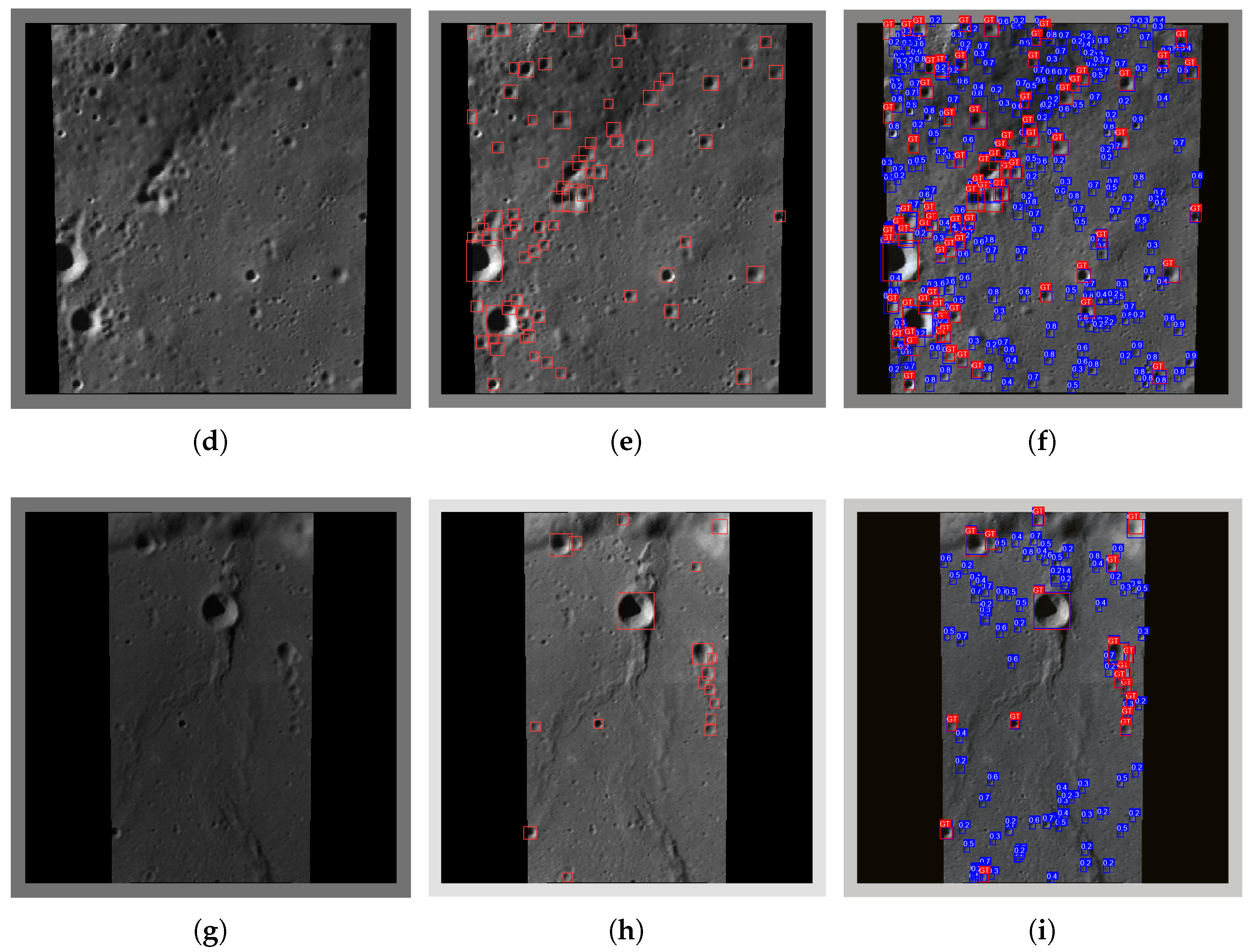
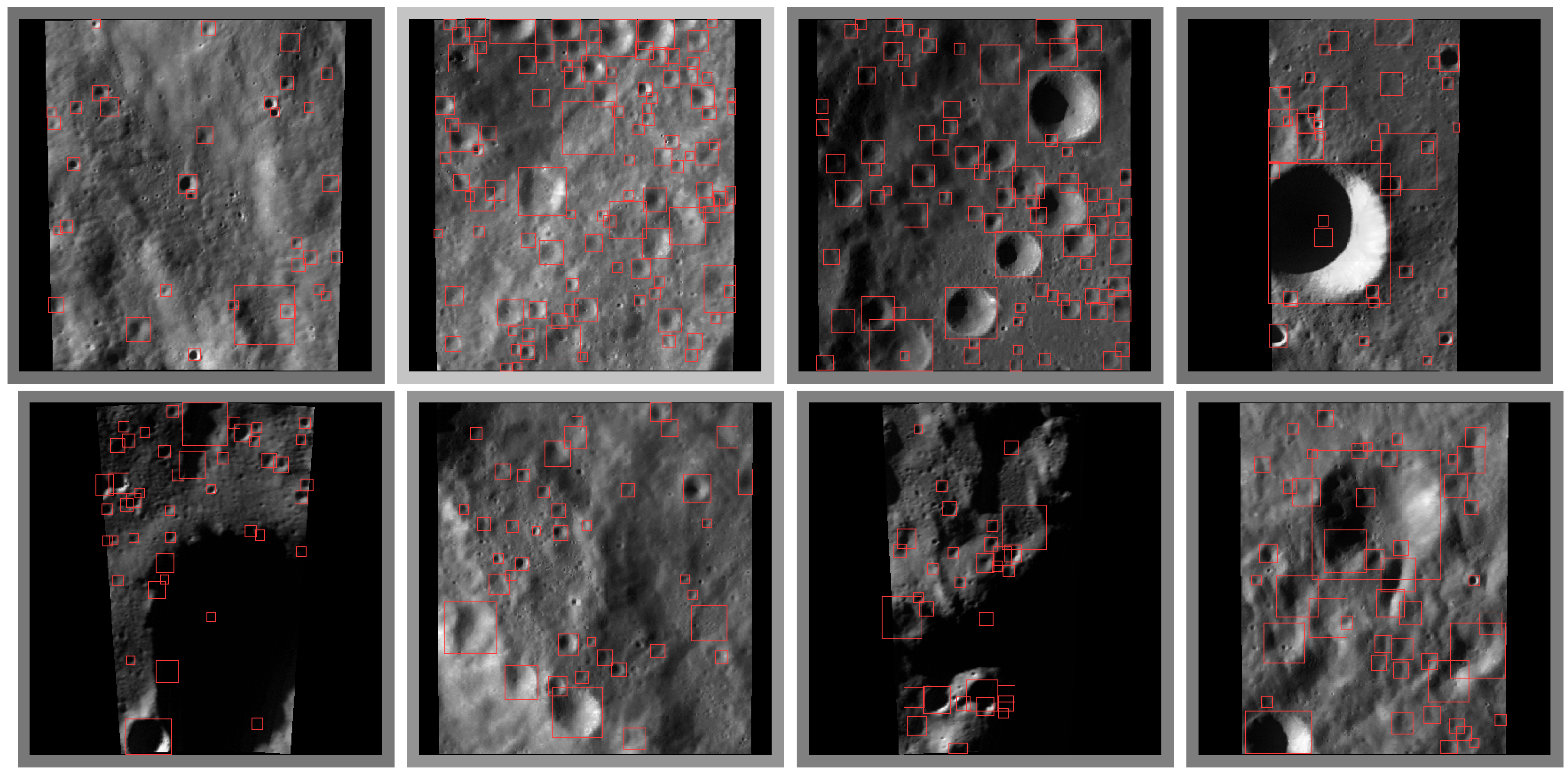
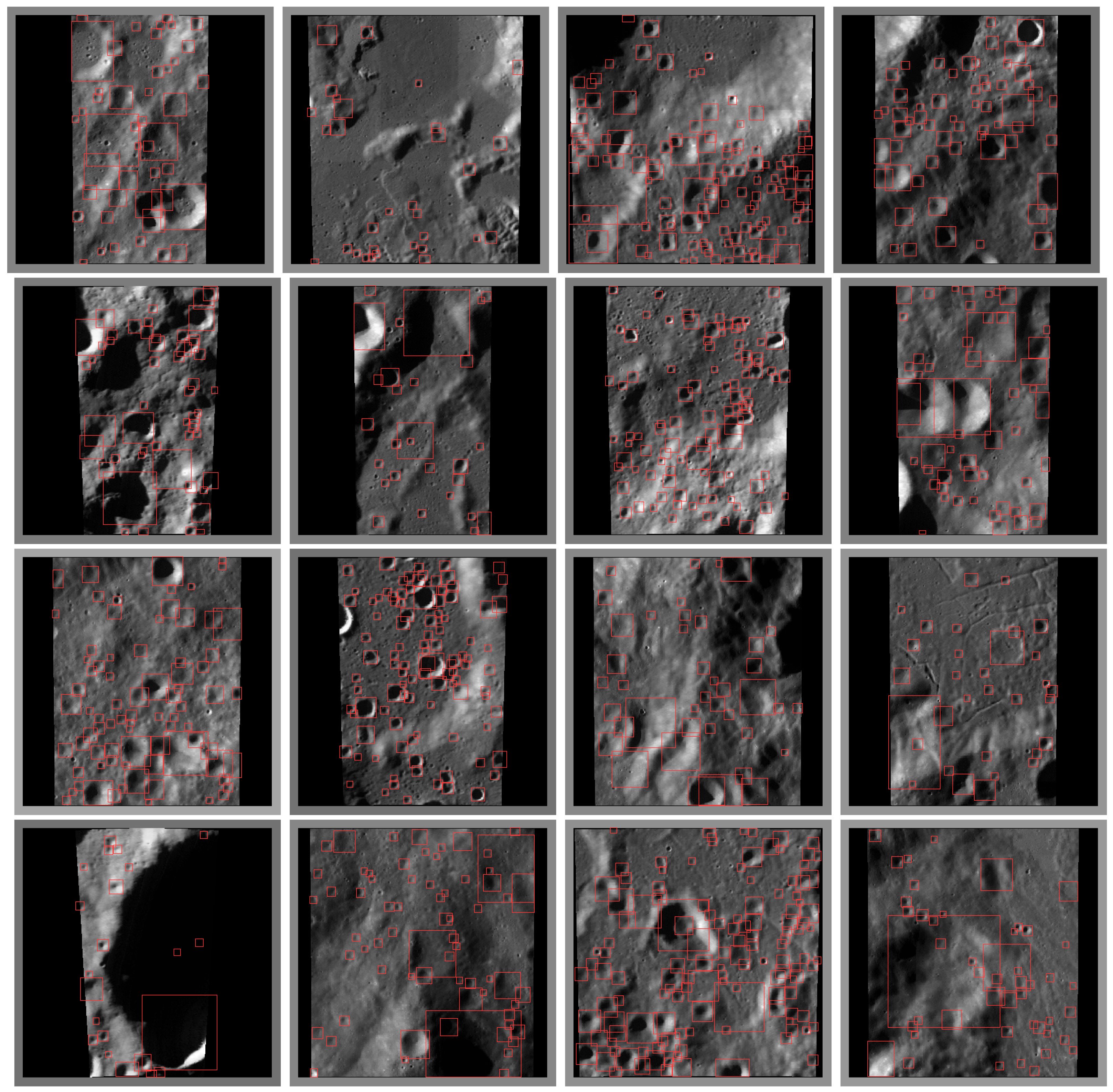
5. Results
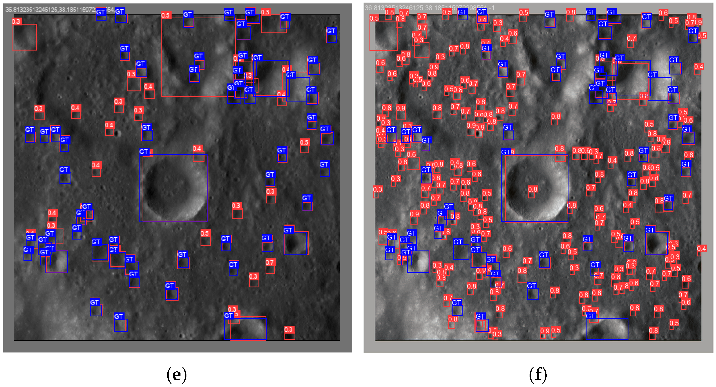
5.1. Quantitative/Qualitative Analysis
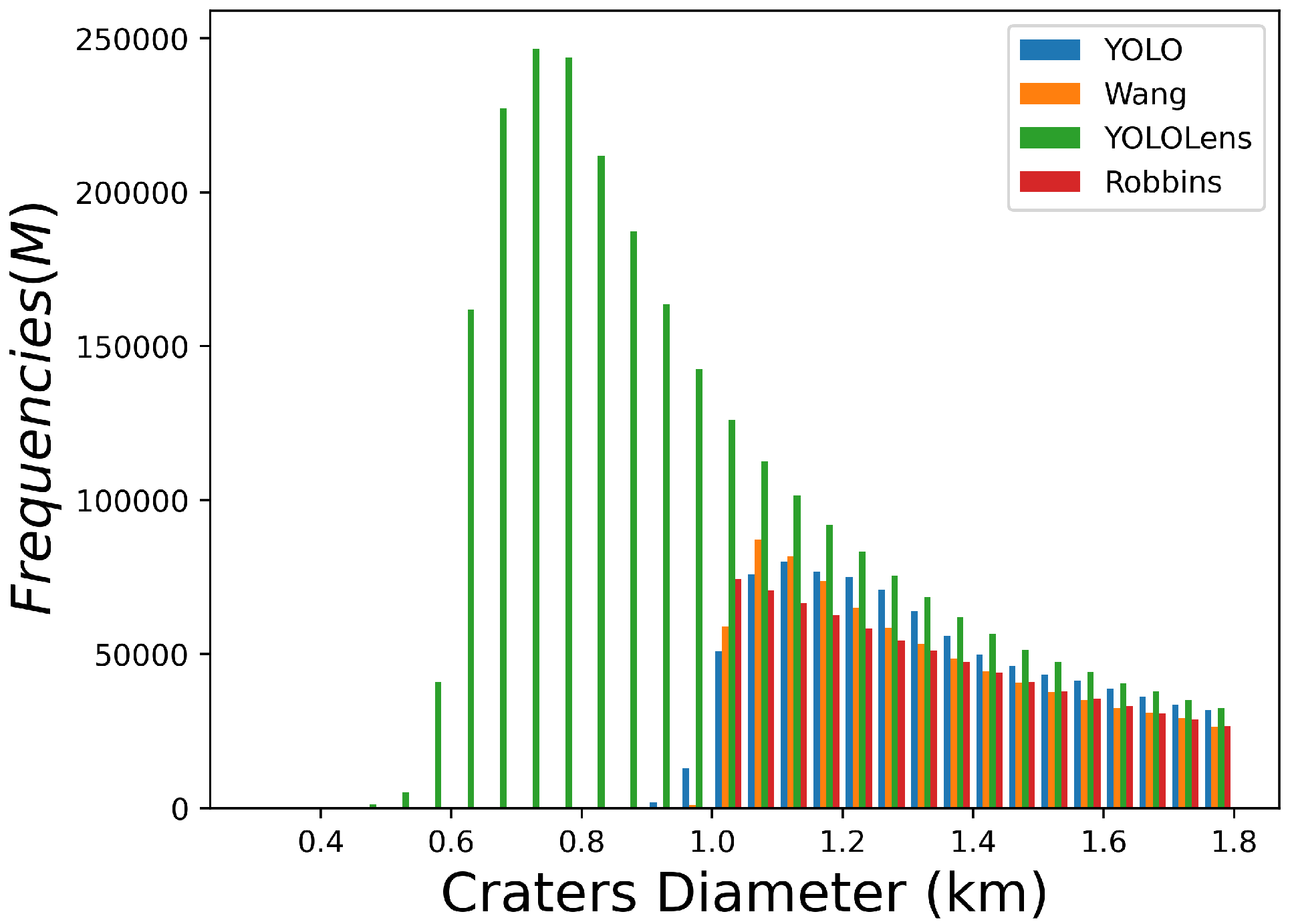
5.1.1. Analysis 1: Model’s Performance per Diameters Crater Range
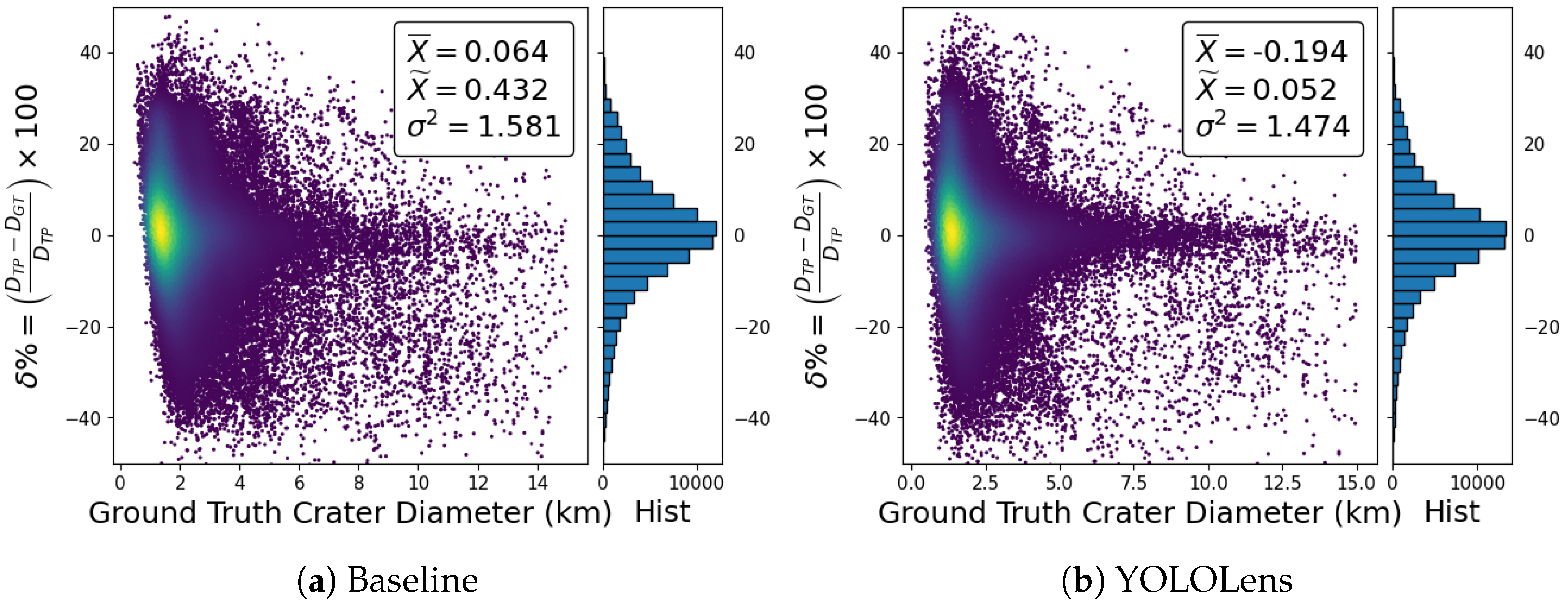
5.1.2. Analysis 2: Crater Diameter Error
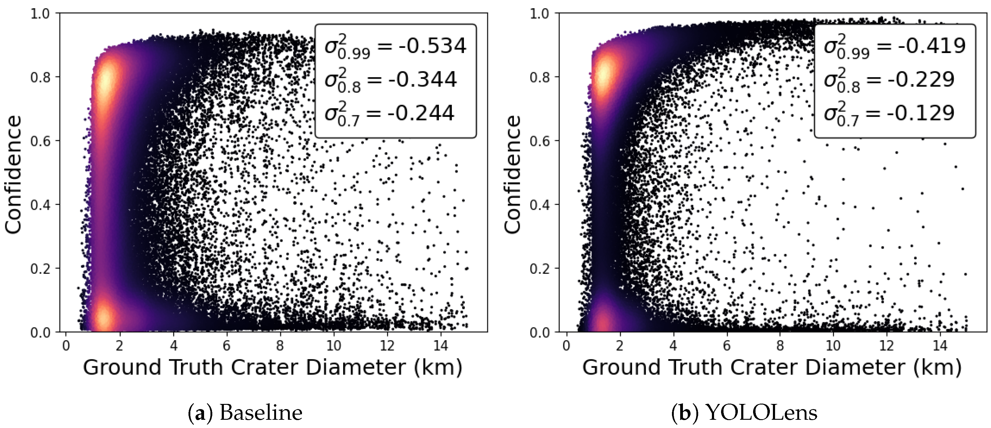
5.1.3. Analysis 3: The Performance’s Impact of the Scale Factor
6. Discussion
- The novel generative/object detection model can produce a super-resolution image, enhancing the capability of the object detection task through an end-to-end model.
- A workflow is developed to the craters georeference on the LROC WAC derived global mosaic, starting from a generic lunar catalog.
- Quantitative and qualitative performance analyzes and comparison with literature, super-resolution impact at different scales for crater detection task, and evaluation per diameter ranges are performed to prove the effectiveness and robustness of the proposed model.
7. Conclusions
Author Contributions
Funding
Data Availability Statement
Conflicts of Interest
Appendix A. Apollo 12 Landing Site


References
- Strom, R.G.; Malhotra, R.; Ito, T.; Yoshida, F.; Kring, D.A. The origin of planetary impactors in the inner solar system. Science 2005, 309, 1847–1850. [Google Scholar] [CrossRef] [PubMed]
- Fassett, C.I.; Minton, D.A. Impact bombardment of the terrestrial planets and the early history of the Solar System. Nat. Geosci. 2013, 6, 520–524. [Google Scholar] [CrossRef]
- Hartmann, W.K. Martian cratering 8: Isochron refinement and the chronology of Mars. Icarus 2005, 174, 294–320. [Google Scholar] [CrossRef]
- Hartmann, W. Discovery of multi-ring basins-Gestalt perception in planetary science. In Proceedings of the Multi-Ring Basins: Formation and Evolution, Houston, TX, USA, 10–12 November 1980; Pergamon Press: Oxford, UK, 1981; pp. 79–90. [Google Scholar]
- Neukum, G.; König, B.; Arkani-Hamed, J. A study of lunar impact crater size-distributions. Moon 1975, 12, 201–229. [Google Scholar] [CrossRef]
- Neukum, G.; Ivanov, B.A. Crater size distributions and impact probabilities on earth from lunar, terrestrial planeta, and asteroid cratering data. In Hazards Due to Comets and Asteroids; University of Arizona Press: Tucson, AZ, USA, 1994; pp. 359–416. [Google Scholar]
- Neukum, G.; Ivanov, B.A.; Hartmann, W.K. Cratering records in the inner solar system in relation to the lunar reference system. In Chronology and Evolution of Mars; Springer: Berlin/Heidelberg, Germany, 2001; pp. 55–86. [Google Scholar]
- Hartmann, W.K. Relative crater production rates on planets. Icarus 1977, 31, 260–276. [Google Scholar] [CrossRef]
- Marchi, S.; Mottola, S.; Cremonese, G.; Massironi, M.; Martellato, E. A new chronology for the Moon and Mercury. Astron. J. 2009, 137, 4936. [Google Scholar] [CrossRef]
- Le Feuvre, M.; Wieczorek, M.A. Nonuniform cratering of the Moon and a revised crater chronology of the inner Solar System. Icarus 2011, 214, 1–20. [Google Scholar] [CrossRef]
- Stoffler, D.; Ryder, G.; Ivanov, B.A.; Artemieva, N.A.; Cintala, M.J.; Grieve, R.A. Cratering history and lunar chronology. Rev. Mineral. Geochem. Mineral. Soc. Am. 2006, 60, 519–596. [Google Scholar] [CrossRef]
- Hiesinger, H.; Head III, J.W. New views of lunar geoscience: An introduction and overview. Rev. Mineral. Geochem. 2006, 60, 1–81. [Google Scholar] [CrossRef]
- Hiesinger, H.; Jaumann, R.; Neukum, G.; Head III, J.W. Ages of mare basalts on the lunar nearside. J. Geophys. Res. Planets 2000, 105, 29239–29275. [Google Scholar] [CrossRef]
- Hiesinger, H.; Head, J.; Wolf, U.; Jaumann, R.; Neukum, G. Ages and stratigraphy of lunar mare basalts: A synthesis. Recent Adv. Curr. Res. Issues Lunar Stratigr. 2011, 477, 1–51. [Google Scholar]
- Benedix, G.; Lagain, A.; Chai, K.; Meka, S.; Anderson, S.; Norman, C.; Bland, P.; Paxman, J.; Towner, M.; Tan, T. Deriving surface ages on Mars using automated crater counting. Earth Space Sci. 2020, 7, e2019EA001005. [Google Scholar] [CrossRef]
- Williams, J.P.; van der Bogert, C.H.; Pathare, A.V.; Michael, G.G.; Kirchoff, M.R.; Hiesinger, H. Dating very young planetary surfaces from crater statistics: A review of issues and challenges. Meteorit. Planet. Sci. 2018, 53, 554–582. [Google Scholar] [CrossRef]
- Gunn, M.; Cousins, C.R. Mars surface context cameras past, present, and future. Earth Space Sci. 2016, 3, 144–162. [Google Scholar] [CrossRef]
- Hu, T.; Yang, Z.; Kang, Z.; Lin, H.; Zhong, J.; Zhang, D.; Cao, Y.; Geng, H. Population of Degrading Small Impact Craters in the Chang’E-4 Landing Area Using Descent and Ground Images. Remote Sens. 2022, 14, 3608. [Google Scholar] [CrossRef]
- Martellato, E.; Vivaldi, V.; Massironi, M.; Cremonese, G.; Marzari, F.; Ninfo, A.; Haruyama, J. Is the Linné impact crater morphology influenced by the rheological layering on the Moon’s surface? Insights from numerical modeling. Meteorit. Planet. Sci. 2017, 52, 1388–1411. [Google Scholar] [CrossRef]
- Michael, G. Planetary surface dating from crater size–frequency distribution measurements: Multiple resurfacing episodes and differential isochron fitting. Icarus 2013, 226, 885–890. [Google Scholar] [CrossRef]
- Neukum, G.; Horn, P. Effects of lava flows on lunar crater populations. Moon 1976, 15, 205–222. [Google Scholar] [CrossRef]
- Prieur, N.C.; Rolf, T.; Wünnemann, K.; Werner, S.C. Formation of simple impact craters in layered targets: Implications for lunar crater morphology and regolith thickness. J. Geophys. Res. Planets 2018, 123, 1555–1578. [Google Scholar] [CrossRef]
- Robbins, S.J.; Antonenko, I.; Kirchoff, M.R.; Chapman, C.R.; Fassett, C.I.; Herrick, R.R.; Singer, K.; Zanetti, M.; Lehan, C.; Huang, D.; et al. The variability of crater identification among expert and community crater analysts. Icarus 2014, 234, 109–131. [Google Scholar] [CrossRef]
- Athanassas, C.; Vaiopoulos, A.; Kolokoussis, P.; Argialas, D. Remote Sensing of Mars: Detection of Impact Craters on the Mars Global Surveyor DTM by Integrating Edge-and Region-Based Algorithms. Earth Moon Planets 2018, 121, 59–72. [Google Scholar] [CrossRef]
- Bue, B.D.; Stepinski, T.F. Machine detection of Martian impact craters from digital topography data. IEEE Trans. Geosci. Remote Sens. 2006, 45, 265–274. [Google Scholar] [CrossRef]
- Christoff, N.; Jorda, L.; Viseur, S.; Bouley, S.; Manolova, A.; Mari, J.L. Automated extraction of crater rims on 3D meshes combining artificial neural network and discrete curvature labeling. Earth Moon Planets 2020, 124, 51–72. [Google Scholar] [CrossRef]
- Di, K.; Li, W.; Yue, Z.; Sun, Y.; Liu, Y. A machine learning approach to crater detection from topographic data. Adv. Space Res. 2014, 54, 2419–2429. [Google Scholar] [CrossRef]
- Fairweather, J.; Lagain, A.; Servis, K.; Benedix, G.; Kumar, S.; Bland, P. Automatic Mapping of Small Lunar Impact Craters Using LRO-NAC Images. Earth Space Sci. 2022, 9, e2021EA002177. [Google Scholar] [CrossRef]
- Hu, Y.; Xiao, J.; Liu, L.; Zhang, L.; Wang, Y. Detection of Small Impact Craters via Semantic Segmenting Lunar Point Clouds Using Deep Learning Network. Remote Sens. 2021, 13, 1826. [Google Scholar] [CrossRef]
- Kang, Z.; Wang, X.; Hu, T.; Yang, J. Coarse-to-fine extraction of small-scale lunar impact craters from the CCD images of the Chang’E lunar orbiters. IEEE Trans. Geosci. Remote Sens. 2018, 57, 181–193. [Google Scholar] [CrossRef]
- Kim, J.R.; Muller, J.P.; van Gasselt, S.; Morley, J.G.; Neukum, G. Automated crater detection, a new tool for Mars cartography and chronology. Photogramm. Eng. Remote Sens. 2005, 71, 1205–1217. [Google Scholar] [CrossRef]
- Lee, C. Automated crater detection on Mars using deep learning. Planet Space Sci. 2019, 170, 16–28. [Google Scholar] [CrossRef]
- Liu, D.; Chen, M.; Qian, K.; Lei, M.; Zhou, Y. Boundary detection of dispersal impact craters based on morphological characteristics using lunar digital elevation model. IEEE J. Sel. Top. Appl. Earth Obs. Remote Sens. 2017, 10, 5632–5646. [Google Scholar] [CrossRef]
- Michael, G. Coordinate registration by automated crater recognition. Planet Space Sci. 2003, 51, 563–568. [Google Scholar] [CrossRef]
- Sawabe, Y.; Matsunaga, T.; Rokugawa, S. Automated detection and classification of lunar craters using multiple approaches. Adv. Space Res. 2006, 37, 21–27. [Google Scholar] [CrossRef]
- Silburt, A.; Ali-Dib, M.; Zhu, C.; Jackson, A.; Valencia, D.; Kissin, Y.; Tamayo, D.; Menou, K. Lunar crater identification via deep learning. Icarus 2019, 317, 27–38. [Google Scholar] [CrossRef]
- Tewari, A.; Verma, V.; Srivastava, P.; Jain, V.; Khanna, N. Automated crater detection from co-registered optical images, elevation maps and slope maps using deep learning. Planet Space Sci. 2022, 218, 105500. [Google Scholar] [CrossRef]
- Zhou, Y.; Zhao, H.; Chen, M.; Tu, J.; Yan, L. Automatic detection of lunar craters based on DEM data with the terrain analysis method. Planet Space Sci. 2018, 160, 1–11. [Google Scholar] [CrossRef]
- Vijayan, S.; Vani, K.; Sanjeevi, S. Crater detection, classification and contextual information extraction in lunar images using a novel algorithm. Icarus 2013, 226, 798–815. [Google Scholar] [CrossRef]
- Fan, L.; Yuan, J.; Zha, K.; Wang, X. ELCD: Efficient Lunar Crater Detection Based on Attention Mechanisms and Multiscale Feature Fusion Networks from Digital Elevation Models. Remote Sens. 2022, 14, 5225. [Google Scholar] [CrossRef]
- Lin, X.; Zhu, Z.; Yu, X.; Ji, X.; Luo, T.; Xi, X.; Zhu, M.; Liang, Y. Lunar Crater Detection on Digital Elevation Model: A Complete Workflow Using Deep Learning and Its Application. Remote Sens. 2022, 14, 621. [Google Scholar] [CrossRef]
- Wang, Y.; Wu, B.; Xue, H.; Li, X.; Ma, J. An Improved Global Catalog of Lunar Impact Craters (≥1 km) with 3D Morphometric Information and Updates on Global Crater Analysis. J. Geophys. Res. Planets 2021, 126, e2020JE006728. [Google Scholar] [CrossRef]
- Shermeyer, J.; Van Etten, A. The effects of super-resolution on object detection performance in satellite imagery. In Proceedings of the IEEE/CVF Conference on Computer Vision and Pattern Recognition Workshops, Long Beach, CA, USA, 16–17 June 2019. [Google Scholar]
- La Grassa, R.; Gallo, I.; Re, C.; Cremonese, G.; Landro, N.; Pernechele, C.; Simioni, E.; Gatti, M. An Adversarial Generative Network Designed for High-Resolution Monocular Depth Estimation from 2D HiRISE Images of Mars. Remote Sens. 2022, 14, 4619. [Google Scholar] [CrossRef]
- Head III, J.W.; Fassett, C.I.; Kadish, S.J.; Smith, D.E.; Zuber, M.T.; Neumann, G.A.; Mazarico, E. Global distribution of large lunar craters: Implications for resurfacing and impactor populations. Science 2010, 329, 1504–1507. [Google Scholar] [CrossRef] [PubMed]
- Povilaitis, R.; Robinson, M.; Van der Bogert, C.; Hiesinger, H.; Meyer, H.; Ostrach, L. Crater density differences: Exploring regional resurfacing, secondary crater populations, and crater saturation equilibrium on the moon. Planet Space Sci. 2018, 162, 41–51. [Google Scholar] [CrossRef]
- Robbins, S.J. A new global database of lunar impact craters> 1–2 km: 1. Crater locations and sizes, comparisons with published databases, and global analysis. J. Geophys. Res. Planets 2019, 124, 871–892. [Google Scholar] [CrossRef]
- Salamunićcar, G.; Lončarić, S.; Grumpe, A.; Wöhler, C. Hybrid method for crater detection based on topography reconstruction from optical images and the new LU78287GT catalogue of Lunar impact craters. Adv. Space Res. 2014, 53, 1783–1797. [Google Scholar] [CrossRef]
- Wetzler, P.G.; Honda, R.; Enke, B.; Merline, W.J.; Chapman, C.R.; Burl, M.C. Learning to detect small impact craters. In Proceedings of the 2005 Seventh IEEE Workshops on Applications of Computer Vision (WACV/MOTION’05), Breckenridge, CO, USA, 5–7 January 2005; IEEE: Piscataway, NJ, USA, 2005; Volume 1, pp. 178–184. [Google Scholar]
- Lee, C.; Hogan, J. Automated crater detection with human level performance. Comput. Geosci. 2021, 147, 104645. [Google Scholar] [CrossRef]
- Cadogan, P.H. Automated precision counting of very small craters at lunar landing sites. Icarus 2020, 348, 113822. [Google Scholar] [CrossRef]
- Dalal, N.; Triggs, B. Histograms of oriented gradients for human detection. In Proceedings of the 2005 IEEE Computer Society Conference on Computer Vision and Pattern Recognition (CVPR’05), San Diego, CA, USA, 20–25 June 2005; IEEE: Piscataway, NJ, USA, 2005; Volume 1, pp. 886–893. [Google Scholar]
- Lowe, D.G. Distinctive image features from scale-invariant keypoints. Int. J. Comput. Vis. 2004, 60, 91–110. [Google Scholar] [CrossRef]
- La Grassa, R.; Gallo, I.; Landro, N. Dynamic decision boundary for one-class classifiers applied to non-uniformly sampled data. In Proceedings of the 2020 Digital Image Computing: Techniques and Applications (DICTA), Melbourne, Australia, 29 November–2 December 2020; IEEE: Piscataway, NJ, USA, 2020; pp. 1–7. [Google Scholar]
- La Grassa, R.; Gallo, I.; Calefati, A.; Ognibene, D. Binary classification using pairs of minimum spanning trees or n-ary trees. In Proceedings of the International Conference on Computer Analysis of Images and Patterns, Salerno, Italy, 3–5 September 2019; Springer: Berlin/Heidelberg, Germany, 2019; pp. 365–376. [Google Scholar]
- Gallo, I.; La Grassa, R.; Landro, N.; Boschetti, M. Sentinel 2 Time Series Analysis with 3D Feature Pyramid Network and Time Domain Class Activation Intervals for Crop Mapping. ISPRS Int. J.-Geo-Inf. 2021, 10, 483. [Google Scholar] [CrossRef]
- Redmon, J.; Divvala, S.; Girshick, R.; Farhadi, A. You only look once: Unified, real-time object detection. In Proceedings of the IEEE Conference on Computer Vision and Pattern Recognition, Las Vegas, NV, USA, 27–30 June 2016; pp. 779–788. [Google Scholar]
- Lin, T.Y.; Dollár, P.; Girshick, R.; He, K.; Hariharan, B.; Belongie, S. Feature pyramid networks for object detection. In Proceedings of the IEEE Conference on Computer Vision and Pattern Recognition, Honolulu, HI, USA, 21–26 July 2017; pp. 2117–2125. [Google Scholar]
- Liu, S.; Qi, L.; Qin, H.; Shi, J.; Jia, J. Path aggregation network for instance segmentation. In Proceedings of the IEEE Conference on Computer Vision and Pattern Recognition, Salt Lake City, UT, USA, 18–23 June 2018; pp. 8759–8768. [Google Scholar]
- Ren, S.; He, K.; Girshick, R.; Sun, J. Faster r-cnn: Towards real-time object detection with region proposal networks. Adv. Neural Inf. Process. Syst. 2015, 28. Available online: https://proceedings.neurips.cc/paper/2015/hash/14bfa6bb14875e45bba028a21ed38046-Abstract.html (accessed on 14 February 2023). [CrossRef]
- Liu, W.; Anguelov, D.; Erhan, D.; Szegedy, C.; Reed, S.; Fu, C.Y.; Berg, A.C. Ssd: Single shot multibox detector. In Proceedings of the European Conference on Computer Vision, Amsterdam, The Netherlands, 11–14 October 2016; Springer: Berlin/Heidelberg, Germany, 2016; pp. 21–37. [Google Scholar]
- Lin, T.Y.; Goyal, P.; Girshick, R.; He, K.; Dollár, P. Focal loss for dense object detection. In Proceedings of the IEEE International Conference on Computer Vision, Venice, Italy, 22–29 October 2017; pp. 2980–2988. [Google Scholar]
- Zhang, Y.; Tian, Y.; Kong, Y.; Zhong, B.; Fu, Y. Residual dense network for image super-resolution. In Proceedings of the IEEE Conference on Computer Vision and Pattern Recognition, Salt Lake City, UT, USA, 18–23 June 2018; pp. 2472–2481. [Google Scholar]
- Speyerer, E.; Robinson, M.; Denevi, B.; LROC Science Team. Lunar Reconnaissance Orbiter Camera global morphological map of the Moon. In Proceedings of the 42nd Annual Lunar and Planetary Science Conference, The Woodlands, TX, USA, 7–11 March 2011; number 1608. p. 2387. [Google Scholar]
- Robinson, M.; Brylow, S.; Tschimmel, M.; Humm, D.; Lawrence, S.; Thomas, P.; Denevi, B.; Bowman-Cisneros, E.; Zerr, J.; Ravine, M.; et al. Lunar reconnaissance orbiter camera (LROC) instrument overview. Space Sci. Rev. 2010, 150, 81–124. [Google Scholar] [CrossRef]
- Wagner, R.; Speyerer, E.; Robinson, M.; LROC Team. New mosaicked data products from the LROC team. In Proceedings of the 46th Annual Lunar and Planetary Science Conference, The Woodlands, TX, USA, 16–20 March 2015; number 1832. p. 1473. [Google Scholar]
- Sato, H.; Robinson, M.; Hapke, B.; Denevi, B.; Boyd, A. Resolved Hapke parameter maps of the Moon. J. Geophys. Res. Planets 2014, 119, 1775–1805. [Google Scholar] [CrossRef]
- Robbins, S.J.; Riggs, J.D.; Weaver, B.P.; Bierhaus, E.B.; Chapman, C.R.; Kirchoff, M.R.; Singer, K.N.; Gaddis, L.R. Revised recommended methods for analyzing crater size-frequency distributions. Meteorit. Planet. Sci. 2018, 53, 891–931. [Google Scholar] [CrossRef]
- Barker, M.; Mazarico, E.; Neumann, G.; Zuber, M.; Haruyama, J.; Smith, D. A new lunar digital elevation model from the Lunar Orbiter Laser Altimeter and SELENE Terrain Camera. Icarus 2016, 273, 346–355. [Google Scholar] [CrossRef]
- Kingma, D.P.; Ba, J. Adam: A method for stochastic optimization. arXiv 2014, arXiv:1412.6980. [Google Scholar]
- Wang, S.; Fan, Z.; Li, Z.; Zhang, H.; Wei, C. An effective lunar crater recognition algorithm based on convolutional neural network. Remote Sens. 2020, 12, 2694. [Google Scholar] [CrossRef]
- Zhou, L.; Zhang, C.; Wu, M. D-LinkNet: LinkNet with pretrained encoder and dilated convolution for high resolution satellite imagery road extraction. In Proceedings of the IEEE Conference on Computer Vision and Pattern Recognition Workshops, Salt Lake City, UT, USA, 18–22 June 2018; pp. 182–186. [Google Scholar]
- Orsic, M.; Kreso, I.; Bevandic, P.; Segvic, S. In defense of pre-trained imagenet architectures for real-time semantic segmentation of road-driving images. In Proceedings of the IEEE/CVF Conference on Computer Vision and Pattern Recognition, Long Beach, CA, USA, 15–20 June 2019; pp. 12607–12616. [Google Scholar]
- Cai, Z.; Vasconcelos, N. Cascade r-cnn: Delving into high quality object detection. In Proceedings of the IEEE Conference on Computer Vision and Pattern Recognition, Salt Lake City, UT, USA, 18–23 June 2018; pp. 6154–6162. [Google Scholar]
- Redmon, J.; Farhadi, A. Yolov3: An incremental improvement. arXiv 2018, arXiv:1804.02767. [Google Scholar]
- Kong, T.; Sun, F.; Liu, H.; Jiang, Y.; Li, L.; Shi, J. Foveabox: Beyound anchor-based object detection. IEEE Trans. Image Process. 2020, 29, 7389–7398. [Google Scholar] [CrossRef]
- Tian, Z.; Shen, C.; Chen, H.; He, T. Fcos: Fully convolutional one-stage object detection. In Proceedings of the IEEE/CVF International Conference on Computer Vision, Long Beach, CA, USA, 15–20 June 2019; pp. 9627–9636. [Google Scholar]
- Yang, Z.; Liu, S.; Hu, H.; Wang, L.; Lin, S. Reppoints: Point set representation for object detection. In Proceedings of the IEEE/CVF International Conference on Computer Vision, Long Beach, CA, USA, 15–20 June 2019; pp. 9657–9666. [Google Scholar]
- Iqbal, W.; Hiesinger, H.; van der Bogert, C.H. Geological mapping and chronology of lunar landing sites: Apollo 12. Icarus 2020, 352, 113991. [Google Scholar] [CrossRef]
- Robbins, S.J. New crater calibrations for the lunar crater-age chronology. Earth Planet. Sci. Lett. 2014, 403, 188–198. [Google Scholar] [CrossRef]


| Model Type Comparison | P | R | mAP50 | mAP95 |
|---|---|---|---|---|
| YOLOv5l Baseline | 0.809 | 0.748 | 0.857 | 0.532 |
| YOLOv5x Baseline | 0.82 | 0.76 | 0.866 | 0.539 |
| YOLOLens5x | 0.899 | 0.872 | 0.940 | 0.61 |
| Model Type Comparison | P | R | Params (M) | |
|---|---|---|---|---|
| DeepMoon [36] | 0.810 | 0.560 | 8.0% | 10.3 |
| ERU-Net [71] | 0.754 | 0.812 | 7.8% | 23.7 |
| D-LinkNet [72] | 0.772 | 0.682 | 7.3% | 21.0 |
| SwiftNet [73] | 0.771 | 0.526 | 13.2% | 11.8 |
| ELCD [40] | 0.806 | 0.819 | 6.6% | 21.8 |
| RCNN+FPN [41] | 0.809 | 0.812 | 6.0% | 41.5 |
| YOLOv5l Baseline | 0.809 | 0.748 | 2.37% | 46.1 |
| YOLOv5x Baseline | 0.820 | 0.760 | 2.34% | 86.1 |
| YOLOLens5x | 0.899 | 0.872 | 2.20% | 101.2 |
| Range Km | () | () | () | () |
|---|---|---|---|---|
| No Filter | 0.82 (0.899) | 0.76 (0.872) | 0.866 (0.941) | 0.54(0.617) |
| [1–2) | 0.748 (0.841) | 0.72 (0.82) | 0.78 (0.84) | 0.458 (0.5) |
| [2–3) | 0.747 (0.822) | 0.667 ( 0.783) | 0.691 ( 0.767) | 0.47 ( 0.554) |
| [3–5) | 0.79 ( 0.903) | 0.718 ( 0.855) | 0.761 ( 0.868) | 0.553 ( 0.7) |
| [5–10) | 0.815 ( 0.923) | 0.71 ( 0.892) | 0.793 ( 0.917) | 0.608 ( 0.803) |
| [10–15] | 0.771 ( 0.946) | 0.621 ( 0.866) | 0.701 ( 0.912) | 0.55 ( 0.827) |
| [1–15] | 0.82 ( 0.911) | 0.765 ( 0.879) | 0.868 ( 0.938) | 0.541 ( 0.62) |
| Method | AP (IoU Threshold ) Range [5–10 km) |
|---|---|
| RCNN [60] | 0.843 |
| RCNN + FPN [58] | 0.839 |
| Cascade RCNN [74] | 0.822 |
| SSD [61] | 0.804 |
| RetinaNet [62] | 0.655 |
| YOLOv3 [75] | 0.729 |
| FoveaBox [76] | 0.803 |
| FCOS [77] | 0.829 |
| RepPoints [78] | 0.793 |
| YOLOLens5x | 0.917 |
| Method | P | R | mAP50 | mAP95 |
|---|---|---|---|---|
| YOLO5x SF = 2 | 0.667 | 0.361 | 0.435 | 0.255 |
| YOLOLens5x SF = 4 | 0.807 | 0.697 | 0.79 | 0.446 |
| YOLO5x SF = 1 | 0.82 | 0.76 | 0.866 | 0.539 |
| YOLOLens5x SF = 2 | 0.903 | 0.859 | 0.938 | 0.611 |
Disclaimer/Publisher’s Note: The statements, opinions and data contained in all publications are solely those of the individual author(s) and contributor(s) and not of MDPI and/or the editor(s). MDPI and/or the editor(s) disclaim responsibility for any injury to people or property resulting from any ideas, methods, instructions or products referred to in the content. |
© 2023 by the authors. Licensee MDPI, Basel, Switzerland. This article is an open access article distributed under the terms and conditions of the Creative Commons Attribution (CC BY) license (https://creativecommons.org/licenses/by/4.0/).
Share and Cite
La Grassa, R.; Cremonese, G.; Gallo, I.; Re, C.; Martellato, E. YOLOLens: A Deep Learning Model Based on Super-Resolution to Enhance the Crater Detection of the Planetary Surfaces. Remote Sens. 2023, 15, 1171. https://doi.org/10.3390/rs15051171
La Grassa R, Cremonese G, Gallo I, Re C, Martellato E. YOLOLens: A Deep Learning Model Based on Super-Resolution to Enhance the Crater Detection of the Planetary Surfaces. Remote Sensing. 2023; 15(5):1171. https://doi.org/10.3390/rs15051171
Chicago/Turabian StyleLa Grassa, Riccardo, Gabriele Cremonese, Ignazio Gallo, Cristina Re, and Elena Martellato. 2023. "YOLOLens: A Deep Learning Model Based on Super-Resolution to Enhance the Crater Detection of the Planetary Surfaces" Remote Sensing 15, no. 5: 1171. https://doi.org/10.3390/rs15051171
APA StyleLa Grassa, R., Cremonese, G., Gallo, I., Re, C., & Martellato, E. (2023). YOLOLens: A Deep Learning Model Based on Super-Resolution to Enhance the Crater Detection of the Planetary Surfaces. Remote Sensing, 15(5), 1171. https://doi.org/10.3390/rs15051171