Two-Branch Convolutional Neural Network with Polarized Full Attention for Hyperspectral Image Classification

Abstract

In recent years, convolutional neural networks (CNNs) have been introduced for pixel-wise hyperspectral image (HSI) classification tasks. However, some problems of the CNNs are still insufficiently addressed, such as the receptive field problem, small sample problem, and feature fusion problem. To tackle the above problems, we proposed a two-branch convolutional neural network with a polarized full attention mechanism for HSI classification. In the proposed network, two-branch CNNs are implemented to efficiently extract the spectral and spatial features, respectively. The kernel sizes of the convolutional layers are simplified to reduce the complexity of the network. This approach can make the network easier to be trained and fit the network to small sample size conditions. The one-shot connection technique is applied to improve the efficiency of feature extraction. An improved full attention block, named polarized full attention, is exploited to fuse the feature maps and provide global contextual information. Experimental results on several public HSI datasets confirm the effectiveness of the proposed network.

1. Introduction

Hyperspectral image (HSI) is collected by the remote sensor on the surface of the earth, which consists of hundreds of narrow electromagnetic spectrums from the visible to the near-infrared wavelength ranges. Since the HSI can distinguish subtle variations from the spectral signatures of the land cover object, it has been widely applied in many fields, such as urban planning [1], fine agriculture [2], and mineral exploration [3]. However, the complex statistical and geometrical properties of HSI datasets prevent the direct utilization of traditional analysis techniques for multispectral images to extract meaningful information from hyperspectral ones. As a result, many scholars focus on developing analysis techniques of artificial intelligence specifically for HSI datasets.

HSI classification is an important analysis technique in the hyperspectral community, which assigns each pixel of HSI to one certain class based on its spectral signatures [4]. Traditional HSI classification techniques focus on exploring the shallow characteristics of the HSI dataset to extract discriminable information, such as the principal component analysis (PCA) [5], independent component analysis (ICA) [6], and linear discriminate analysis (LDA) [7]). After that, machine learning techniques are used to classify the discriminable information of the HSI dataset, such as the support vector machines (SVMs) [8], multinomial logistic regression [9], and extreme learning machines (ELMs) [10,11]. These methods design hand-crafted descriptors for specific tasks to explore features, which depends on expert knowledge in the parameter setup phase. However, the expert knowledge is difficult to access in practice, which limits the applicability of these methods to process a large amount of heterogeneous HSI datasets in a consistent end-to-end manner.

In recent years, deep learning techniques have shown great potential in computer vision tasks, such as image classification [12], object detection [13], and semantic segmentation [14]. Motivated by those successful applications, deep learning techniques have been introduced to HSI classification tasks. Different from the traditional HSI classification approaches, the deep learning techniques adaptively and hierarchically explore information from the original HSI dataset and obtain the shallow texture features and deep semantic features via different neural network layers. The parameters of the deep learning techniques can be learned automatically, which makes these approaches more suitable to deal with complex situations of HSI classification without expert knowledge and solve problems in a consistent manner.

Recently, many deep learning frameworks have been proposed, such as stacked auto-encoders (SAEs) [15], deep belief networks (DBNs) [16], convolutional neural networks (CNNs) [17], recurrent neural networks (RNNs) [18], and generative adversarial networks (GANs) [19]. Among these frameworks, CNNs have achieved good performance in HSI classification and received great favor from scholars. The CNNs use convolutional layers to extract discriminable information from HSI and apply the weight-share mechanism to reduce the complexity of the network. According to the extracted features, the CNNs can be divided into spectral-based CNNs, spatial-based CNNs, and spectral–spatial-based CNNs. Specifically, the spectral-based CNNs focus on extracting informative features from the spectral signatures of HSI, whose input data are always a 1-dimensional (1D) vector. For example, Li et al. [20] propose a pixel-pair method that is used to construct the testing pixel and make deep CNN learn pixel-pair features for more discriminative power. Gao et al. [21] propose a CNN architecture for fully utilizing the spectral information of HSI data. Each 1D spectral vector that corresponds to a pixel is transformed into a 2-dimensional (2D) spectral feature matrix. The convolutional layers with $1\times 1$ and $3\times 3$ window sizes are used to extract the spectral features jointly. It can extract high-level features from HSI data meticulously and comprehensively solve the overfitting problem. The spatial-based CNNs are adept at extracting spatial information of HSI, and the input data are always a 2D matrix. For example, Zhao et al. [22] propose a CNN framework to classify the HSI. Dimension reduction and deep learning techniques are used in the method. A convolutional neural network is utilized to automatically find spatial-related features at high levels. In [23], a CNN system embedded with an extracted hashing feature is proposed for HSI classification. The spectral–spatial CNNs explore either spectral information or spatial information and can extract joint spectral–spatial-based information from the HSI dataset. The input data of the spectral–spatial-based CNN is always a 3-dimensional (3D) tensor. 3D convolutional layers are implemented to extract the discriminative information. For example, Li et al. [24] propose a 3D-CNN framework that views the HSI cube data altogether without relying on any preprocessing or post-processing, extracting the deep spectral–spatial features. Paoletti et al. [25] propose a 3D network to extract spectral and spatial information. The proposed network implements a border mirroring strategy to effectively process border areas in the image and can be efficiently implemented using graphics processing units. Roy et al. [26] propose a bilinear fusion CNN network named FuSENet that fuses SENet with the residual unit. Jia et al. [27] propose a lightweight CNN for HSI classification. Spatial–spectral Schrodinger eigenmaps and dual-scale convolution modules are implemented to extract spatial–spectral features. These CNN-based methods have achieved more positive classification results than the traditional hand-craft classification methods. However, CNNs suffer from gradient vanishing/exploding [28] and network degradation [29] when the networks are designed to be deeper. In addition, the CNNs are also restricted by the window size of the convolutional layers, also known as the receptive field problem, which makes the CNNs to be deficient in the ability to acquire global contextual information.

To solve the gradient vanishing/exploding and network degradation problems, residual connection [30] and dense connection [31,32] are proposed to improve the CNNs. For example, Song et al. [33] propose a deep feature fusion network for HSI classification. The residual learning is introduced to optimize the convolutional layers to make the network easy to be trained. In [34], a new deep CNN architecture is presented specially designed for HSI data. The residual-based approach is used to group the pyramidal bottleneck residual blocks to involve more locations as the network depth increases and balances the workload among all convolutional units. Li et al. [35] propose a two-branch CNN framework, and a dense connection is introduced to maintain the shallow features in the network. In addition, Batch Normalization (BN) [36] and ReLU [37] are applied to suppress the gradient vanishing/exploding problems. For instance, a high-performance two-stream spectral–spatial residual network is proposed for HSI classification in [38]. The network employs a spectral residual network stream to extract spectral characteristics and uses a spatial residual network stream to extract spatial features. The BN layer is used to speed up the training process and improve accuracy. Experiments show that the proposed architecture can be trained with small-size datasets and outperforms the state-of-the-art methods in terms of overall accuracy. Banerjee et al. [39] propose a 3D convolutional neural network together with BN layers to extract the spectral–spatial features from the HSI dataset. The shortcut connections and BN layers are added to get rid of the vanishing gradient problem. Sun et al. propose an improved 3D CNN to solve the problems of overfitting the in-sample training process and the difficulty in highlighting the role of discriminant features. The ReLU is used as a nonlinear activation function to suppress the gradient exploding problem.

To address the receptive field problem, the non-local self-attention methods are invited to capture long-range dependencies of feature maps as global contextual information. For example, Shi et al. [40] propose a double-branch network with pyramidal convolution and iterative attention for HSI classification. In the architecture, the pyramidal convolution and iterative attention mechanism are applied to obtain finer spectral–spatial features to improve the classification performance. Experimental results demonstrate that the proposed model can yield a competitive performance compared to other state-of-the-art models. Li et al. [41] present a spectral–spatial network with channel and position global context attention to capture discriminative features. Two novel global context attentions are proposed to optimize the spectral and spatial features, respectively, for feature enhancement. Experimental results demonstrate that the spectral–spatial network with global context attentions outperforms other related methods. Zhang et al. [42] propose a spectral–spatial self-attention network for HSI classification. The network can adaptively integrate local features with long-range dependencies related to the pixel to be classified. The above approaches effectively improve the CNNs and enhance the ability of CNNs to extract spectral and spatial features from the HSI dataset. However, how to better fuse the extracted spectral and spatial features is still a worthy question to be investigated. Furthermore, the problem of a small sample, which is caused by difficulties in obtaining labeled samples from the HSI dataset, is also a question of concern.

For the multi-feature fusion problem, most of the existing approaches try to feed the features extracted by multiple methods as input data to a fusion model. By fusing the multiple features, the models can extract finer discriminative information, which can help the model to improve the classification capability for HSI classification tasks. For example, Du et al. [43] use the pre-trained CNN models as feature extractors and focus on investigating the performances of different CNN models. The multi-layer feature fusion framework is proposed to integrate multiple level features extracted by a pre-trained CNN model to improve the performance of HSI classification. In [44], several different features are extracted for each pixel of HSI. Then, these features are fed to a deep random forest classifier. With a multiple-layer structure, the outputs of preceding layers will be used as the inputs of the subsequent layers. After the final layer, the classification probability will be computed. Zhang et al. [45] propose a novel method named a specific two-dimensional-tree-dimensional fusion strategy. In the proposed method, two-dimensional convolutional layers and three-dimensional convolutional layers are used to extract rich features of the HSI dataset to keep the spectral and spatial information intact. Then, the spectral and spatial features are fused to classify the HSI dataset. Ma et al. [46] propose a double-branch multi-attention mechanism network for HSI classification. The branches with two types of attention mechanisms are applied to extract multiple features from the HSI dataset. After that, the extracted features are fused for the classification tasks. Li et al. [47] propose an HSI classification method based on octave convolution and multi-scale feature fusion. The octave convolution and attention mechanism are introduced to extract multi-scale features of the HSI dataset. Then, the spectral–spatial fusion features are fused for the classification task.

To address the problem of the small sample, many meaningful efforts have been done in this field. For example, Wang et al. [48] propose to use the ResNet model to extract the ground scene semantics features from high-resolution remote sensing maps with abundant ground objects information, and then classify the GF-2 scene dataset with a small GF-2 data sample through transmigration. Zou et al. [49] propose a graph induction learning method, which has a small parameter space, to solve the problem of a small sample in HSI classification. It treats each pixel of the HSI as a graph node and learns the aggregation function of adjacent vertices through graph sampling and graph aggregation operations to generate the embedding vector of the target vertex. The embedding vectors are used to classify the pixels of the HSI dataset. Wang et al. [50] propose a modified depth-wise separable relational network to deeply capture the similarity between samples. The depth-wise separable convolution is introduced to reduce the computational cost of the model. The Leaky ReLU function is used to improve the training efficiency of the model. The cosine annealing learning rate adjustment strategy is introduced to avoid the model falling into the local optimal solution and enhance the robustness of the model. In [35], a double-branch dual-attention mechanism network is proposed for HSI classification to improve the accuracy and reduce the training samples. Two branches are designed to capture plenty of spectral and spatial features contained in HSI. A channel attention block and a spatial attention block are applied to refine and optimize the extracted feature maps. Pan et al. [51] propose a novel one-shot dense network with polarized attention for HSI classification. In this method, two independent branches are implemented to extract spectral and spatial features, respectively. A channel-only polarized attention mechanism and a spatial-only polarized attention mechanism are applied in the two branches. The polarized attention mechanisms can use a specially designed filtering method to reduce the complexity of the model while maintaining high internal resolution in both channel and spatial dimensions. The above methods solve the small sample problem by pre-training techniques or by reducing the complexity of the classification model. Moreover, data augmentation techniques are also introduced to solve the problem of a small sample. For example, Yu et al. [52] proposed a method to generate labeled samples using the correlation of spectral bands for HSI classification to overcome the small sample problem. In the method, the correlation of spectral bands is fully utilized to generate multiple new sub-samples from each original sample. The number of labeled training samples is thus increased several times. In [53], an auxiliary classifier-based Wasserstein generative adversarial network with gradient penalty is proposed. The framework includes an online generation mechanism and a sample selection algorithm to generate samples that are similar to real data. Experiments on three public HSI datasets show that the proposed framework achieved better classification accuracy with a small number of labeled samples. It is worth noting that the aggressive improvements effectively enhance the performance of the spectral–spatial convolutional neural network frameworks, and the improvements of the convolutional networks are not limited to the above-mentioned methods.

In the proposed framework, a two-branch structure is used to extract the spectral and spatial information of HSI, respectively. By simplifying the window sizes of the 3D convolutional layers, the complexity of the network is reduced to fit the small sample environments. Moreover, a one-shot connection [51] is applied to connect the convolutional layers of the network. This approach allows the shallow features to be maintained in the deeper layers while these features are extracted again jointly with the deep semantic features. The one-shot connection can improve the efficiency of the network in extracting feature maps of different layers and adequately extract the features of the training sample. BN layers and PReLU [54] activation function are implemented in the convolutional layers to suppress the gradient vanishing/exploding problem and network degradation problem. In the proposed architecture, we try to introduce the attention mechanism to solve the problem of feature fusion. We hope to use the attention mechanism to find discriminative abstract features that are worthy of attention. As a result, an improved full attention (FLA) mechanism [55], named polarized full attention (PFLA), is implemented after the two-branch convolutional neural network to extract global contextual information and fuse the spectral and spatial features obtained from the two-branch network. The main contributions are summarized as follows.

(1)

A two-branch neural network is proposed for HSI classification. The two-branch structure is applied to separately extract the spectral and spatial features of HSI. The one-shot connection is used to maintain the shallow features and make the network easy to be trained. The polarized full attention mechanism is implemented to provide global contextual information and fuse the spectral–spatial features.

(2)

An improved full attention mechanism is presented. Sigmoid operation is introduced to obtain the attention weights. This approach can provide polarizability for full attention to keep a high internal resolution when fusing the spectral and spatial features.

(3)

We explore a method that combines the CNN framework and self-attention mechanism for HSI classification and tries to use the attention mechanism to fuse the feature maps. The experimental results on four publicly published HSI datasets are reported.

The rest of the paper is organized as follows. Section 2 introduces the related work of the proposed method. Section 3 gives the details of PTCN. Section 4 collects the experimental results. Section 5 makes some discussions and Section 6 gives the conclusions and future works.

2. Related Work

2.1. Cube-Based Methods for HSI Classification

Traditional pixel-based classification methods only explore the spectral signatures of the HSI dataset and ignore the spatial correlation between pixels. To address this issue, the cube-based method [56,57] is proposed to exploit both spectral and spatial information by constructing cubic samples. To be specific, the input size of the cube-based method is $C\times H\times W$, where $H\times W$ represents the number of neighboring pixels (spatial patch size) and $C$ denotes the number of spectral bands. The cube-based input data is cropped and centered on the corresponding pixel, and its label is determined by its central pixel. The labels of adjacent central pixels are not fed into the network, and we only explore the spatial contextual information around the target pixel.

2.2. Residual Connection, Dense Connection and One-Shot Connection

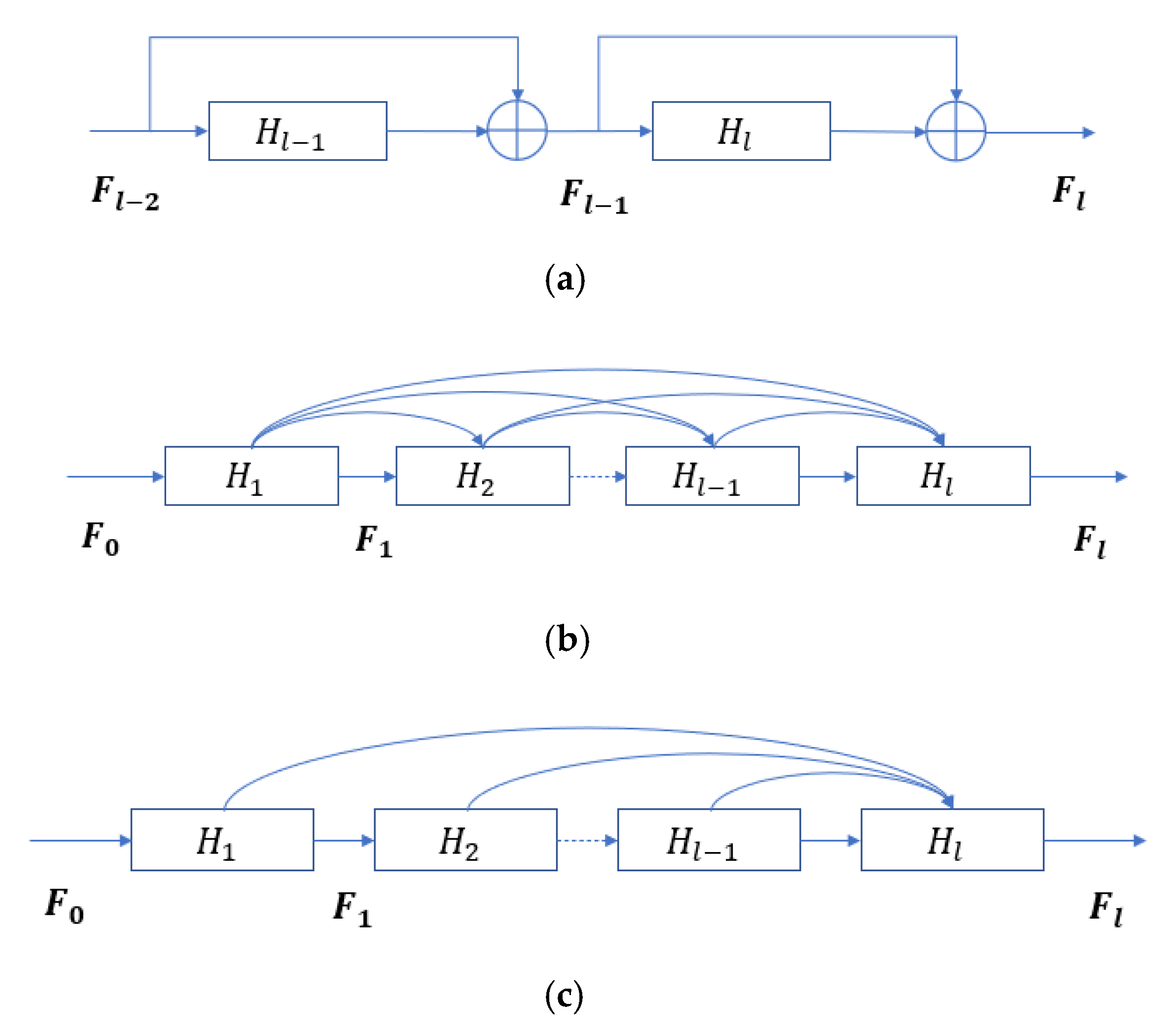
Deep neural networks have emerged as a powerful tool for HSI classification. From the empirical results of experiments, the deeper network models can better extract the abstract features of the HSI dataset to help to improve the classification accuracy. Therefore, scholars tend to design neural network models with more layers. However, with the increase of the depth of the network, the gradient vanishing problem and gradient exploding problem tend to be worse. ResNet [58] first proposes a residual connection to solve this issue. By adding skip connections between different layers, the network can train deeper models to achieve higher accuracy. The ResNet uses a summation operator to combine features to allow the input features to be passed to the subsequent layer. Given $H$ as a hidden layer, $F$ as a feature map, $+$ as a summation operator, the output feature map of the $l$th hidden layer can be expressed as

$$F_l=H_l\left(F_{l-1}\right)+F_{l-1}$$

(1)

However, experiments show that information carried by early feature maps would be washed out as it is summed with others. To better maintain the previous feature maps, DenseNet [59] inherits the concept of skip connection of the ResNet and uses the concatenation operator to combine features in the channel dimension. This approach can preserve the input feature maps in their original forms. All previous feature maps are used to construct the output of the $l$th hidden layer and can be expressed as

$$F_l=H_l\left[F_0, F_1,\dots ,F_{l-1}\right]$$

(2)

Experiments [60] show that the dense connection demonstrates spending more memory and time, and not all connections between layers are positive. Based on the above understanding, methods for connecting between layers are proposed to replace dense connection, such as Log-DenseNet [61], SparseNet [62], HarDNet [63], ThreshNet [64], and VoVnet [65]. In this paper, the one-shot connection is introduced to combine the feature maps, which is proposed by VoVnet. The one-shot connection designs a sparse approach to reduce the number of connections from $L^2$ to $L$ while aggregating all features only once in the last feature maps. This approach outperforms dense connection-based networks with 2$\times$ faster speed and 1.6$\times$–4.1$\times$ energy consumption while providing similar performance. The illustration of the residual connection, dense connection, and one-shot connection is shown in Figure 1.

2.3. Full Attention Mechanism

In recent years, Non-Local (NL) [66]-based methods have achieved great progress by capturing long-range dependencies of feature maps in classification models. They utilize a self-attention mechanism [67,68,69] to explore the interdependencies of the feature maps and obtain linear weights to represent the contributions of the features to reweight the input feature maps. The self-attention mechanism [70] can address the receptive field problem of the standard convolutional network and has shown great potential in HSI classification tasks.

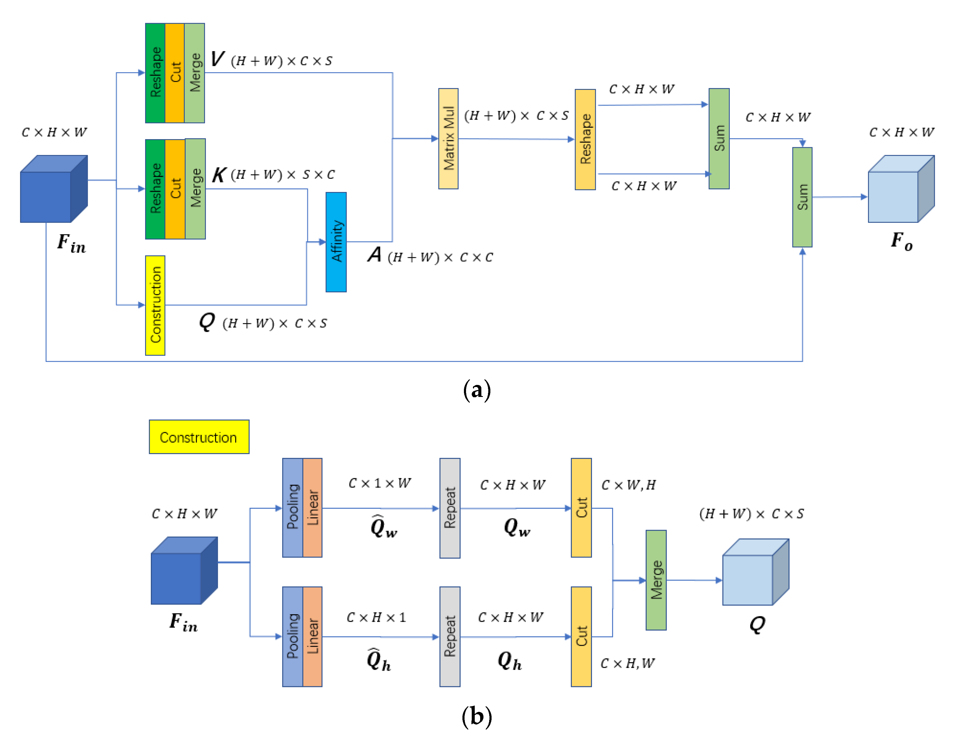
The existing self-attention mechanisms explore the dependencies along the channel or spatial dimensions to obtain corresponding attention weights. However, the integrity of 3D contextual information is missed along the unilateral processing and thus, both channel and spatial NL variants can only benefit partially in a complementary way. To efficiently retain attention in all dimensions in a single attention unit, a non-local block, namely, the Fully Attentional block, is proposed. It utilizes global contextual information to receive spatial responses when computing the channel attention map. The workflow of FLA is shown in Figure 2a.

Given an input feature map $F_{in}\in {ℝ}^{C\times H\times W}$, where $C$ is the number of channels, $H\times W$ is the spatial size of the input feature map and $H$ equals $W$. First, the feature maps $V$ are generated by reshape, cut, and merge operations. The $F_{in}$ is cut along the $H$ dimension to obtain a group of $H$ slices with the size of ${ℝ}^{C\times W}$. Similarly, the $F_{in}$ is cut along the $W$ dimension and obtains a group of $W$ slices with the size of ${ℝ}^{C\times H}$. Then, these two groups are merged to form the feature maps $V\in {ℝ}^{\left(H+W\right)\times S\times C}$, where $S$ equals $H$ and $W$. Second, the feature maps $K\in {ℝ}^{\left(H+W\right)\times C\times S}$ are generated in the same way. Third, the $F_{in}$ is fed into the Construction operation to generate the feature maps $Q$. The workflow of the construction operation is shown in Figure 2b. The construction operation contains two parallel pathways, each of which contains a global average pooling layer followed by a Linear layer. The sizes of the pooling windows are set to $H\times 1$ and $1\times W$ in these two pathways, respectively. By these pooling windows, ${\widehat{Q}}_w\in {ℝ}^{C\times 1\times W}$ and ${\widehat{Q}}_h\in {ℝ}^{C\times H\times 1}$ are obtained. After that, ${\widehat{Q}}_w$ and ${\widehat{Q}}_h$ are repeated to form global features $Q_w\in {ℝ}^{C\times H\times W}$ and $Q_h\in {ℝ}^{C\times H\times W}$. We can see that the $Q_w$ and $Q_h$ represent the global priors in the horizontal and vertical directions, respectively. They can be used to achieve spatial interactions in the corresponding dimension. Next, we cut the $Q_w$ and $Q_h$ along the $H$ and $W$ dimension and merge these slices to form the final global contexts $Q\in {ℝ}^{\left(H+W\right)\times C\times S}$.

After that, $K$ and $Q$ are used to capture the full attentions $A\in {ℝ}^{\left(H+W\right)\times C\times C}$ via the Affinity operation. The Affinity operation is defined as follows:

$$A_{i,j}=\frac{\exp \left(Q_i·K_j\right)}{{\sum }_{i=1}^C\exp \left(Q_i·K_j\right)}$$

(3)

where $A_{i,j}\in A$ denotes the degree of correlation between the $i^{th}$ and $j^{th}$ channel at a specific spatial position. Then, the full attentions $A$ are used to update the channel maps $V$ via matrix multiplication. After that, FLA reshapes the result into two groups and these two groups are summed to form the long-range contextual information. Finally, the output $F_o\in {ℝ}^{C\times H\times W}$ is obtained by an element-wise sum operation between the input feature map $F_{in}$ and the contextual information by multiplying with a scale parameter $\gamma$. The formula can be expressed as follows:

$$F_{o_j}=\gamma {\sum }_{i=1}^C{A}_{i,j}·V_j+F_{i{n}_j}$$

(4)

where $F_{o_j}$ is a feature vector in the output feature map $F_o$ at the $j^{th}$ channel map.

3. Methodology

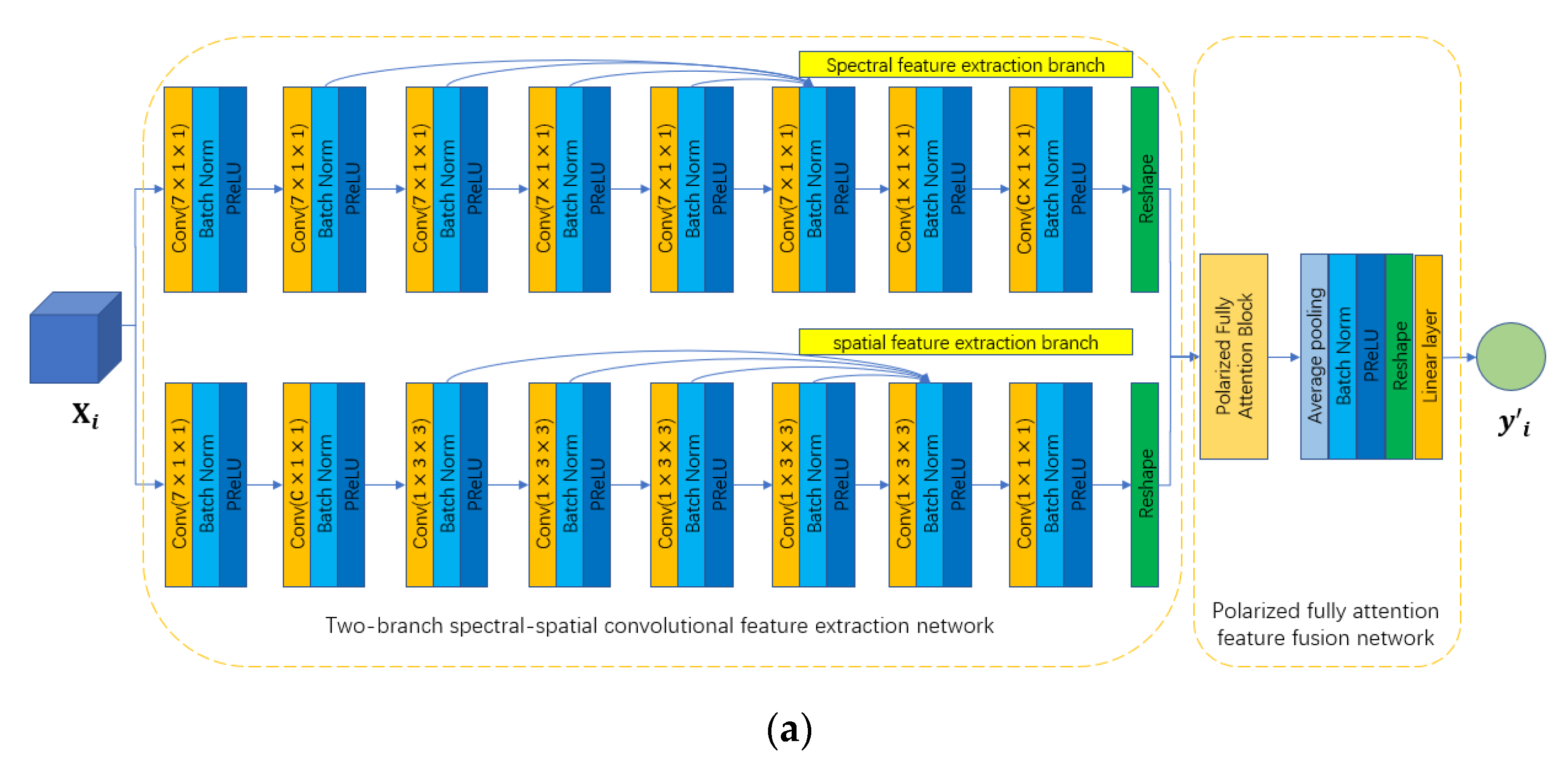
In this paper, we propose a two-branch deep neural network to extract the abundant spectral and spatial information of HSI. The workflow of the proposed network is shown in Figure 3a. We can see that the proposed network is composed of two components: the two-branch spectral–spatial convolutional feature extraction network and the polarized full attention feature fusion network.

In the two-branch spectral–spatial convolutional feature extraction network, a two-branch structure is used to individually extract the spectral and spatial information along the spectral and spatial dimensions, respectively. Given an input dataset $X_i\in {ℝ}^{D\times C\times H\times W}$, where $X_i$ is the cube-based HSI data of the $i^{th}$ pixel, $D$ is the number of feature maps ($D$ is set to 1 when initializing the input dataset), $C$ is the number of spectral dimensions, $H\times W$ is the size of the spatial dimensions, the output of the network is $y_i^{\prime }\in {ℝ}^{1\times m}$, where $m$ is the number of land cover categories. The spectral feature extraction branch contains eight convolutional layers with the BN layer and PReLU activation function layer. First, we employ a convolutional layer with window size $7\times 1\times 1$ to reduce the spectral dimension and increase the number of feature maps. After that, five convolutional layers with a $7\times 1\times 1$ window size are used to further extract the spectral information. A one-shot connection is implemented among these convolutional layers to maintain the previous feature maps. Next, a convolutional layer with a $1\times 1\times 1$ window size is deployed to compress the feature maps. Furthermore, a convolutional layer with a $C\times 1\times 1$ window size and reshape operation are used to squeeze the spectral dimension. Similarly, the spatial feature extraction branch employs eight convolutional layers with BN and PReLU to extract the spatial information. First, a convolutional layer with a $7\times 1\times 1$ window size is implemented to reduce the spectral dimension and increase the number of feature maps. After that, a convolutional layer with a $C\times 1\times 1$ window size is used to compress the spectral dimension. Next, five convolutional layers with a $1\times 3\times 3$ window size are applied to extract the spatial information. A one-shot connection is carried out among these convolutional layers to maintain the information. After that, a convolutional layer with a $1\times 1\times 1$ window size and reshape operation are conducted to compress the number of feature maps and squeeze the spectral dimension. Finally, the outputs of the spectral branch and spatial branch are concatenated to form the final feature maps.

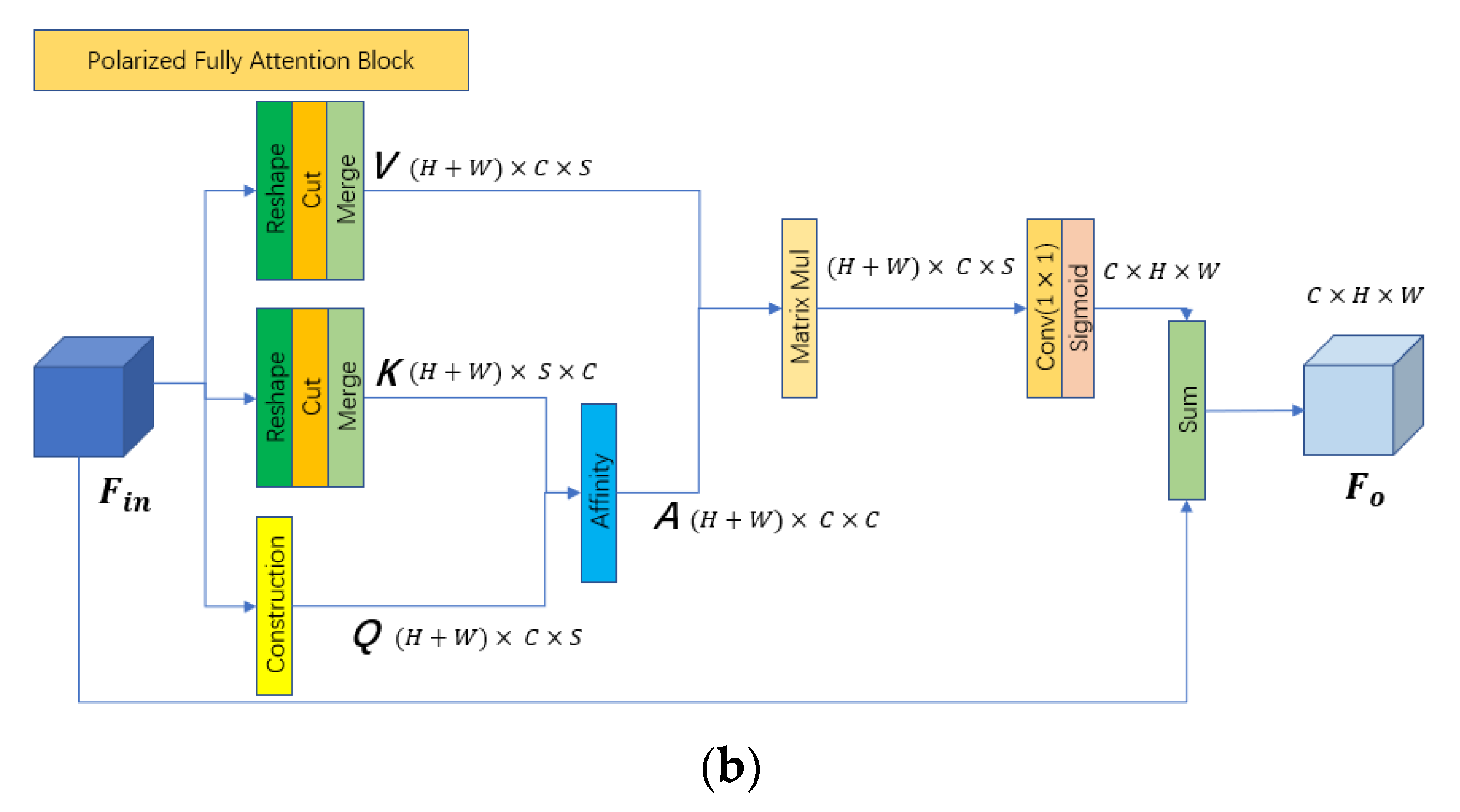
The polarized full attention feature fusion network is deployed after the two-branch spectral–spatial convolutional feature extraction network and is used to fuse the previous feature maps to generate the final classification results. From Figure 3a, we can see that the polarized full attention feature fusion network is composed of PFLA, an average pooling layer with a BN layer, PReLU activation function layer, reshape operation, and Linear layer. First, the PFLA is implemented to further extract interesting information from the feature maps extracted by the previous two-branch network by the self-attention mechanism. Different from the traditional FLA, the proposed PFLA employs a convolutional layer with a $1\times 1$ window size to generate the global contextual information and use the Sigmoid operation to provide polarizability to keep high internal resolution when fusing the channel-wise attentions. The workflow of the PFLA is shown in Figure 3b. We can see that most of the processes of PFLA are the same as the FLA, with the difference that the convolutional layer and Sigmoid operation are deployed after the matrix multiplication of $V$ and $A$. Next, an average pooling layer with BN layer and PReLU activation function layer is conducted to compress the spatial dimension and fuse the features. Finally, a reshape operation is used to squeeze the spatial dimension, and a Linear layer is used to generate the final classification results. To illustrate the details of the proposed network, the dataflows of the two-branch spectral–spatial convolutional feature extraction network and polarized full attention feature fusion network are shown in

Table 1. The dataflow of the spectral feature extraction branch.

Input Size	Layer Name	Kernel	Stride	Padding	Filters	Output Size
$\left(1,103,9,9\right)$	Conv	$\left(7,1,1\right)$	$\left(3,1,1\right)$	$\left(0,0,0\right)$	$24$	$\left(24,49,9,9\right)$
$\left(24,49,9,9\right)$	Conv	$\left(7,1,1\right)$	$\left(1,1,1\right)$	$\left(3,0,0\right)$	$24$	$\left(24,49,9,9\right)$
$\left(24,49,9,9\right)$	Conv	$\left(7,1,1\right)$	$\left(1,1,1\right)$	$\left(3,0,0\right)$	$24$	$\left(24,49,9,9\right)$
$\left(24,49,9,9\right)$	Conv	$\left(7,1,1\right)$	$\left(1,1,1\right)$	$\left(3,0,0\right)$	$24$	$\left(24,49,9,9\right)$
$\left(24,49,9,9\right)$	Conv	$\left(7,1,1\right)$	$\left(1,1,1\right)$	$\left(3,0,0\right)$	$24$	$\left(24,49,9,9\right)$
$\left(24,49,9,9\right)$	Conv	$\left(7,1,1\right)$	$\left(1,1,1\right)$	$\left(3,0,0\right)$	$24$	$\left(120,49,9,9\right)$
$\left(120,49,9,9\right)$	Conv	$\left(1,1,1\right)$	$\left(1,1,1\right)$	$\left(0,0,0\right)$	$24$	$\left(24,49,9,9\right)$
$\left(24,49,9,9\right)$	Conv	$\left(49,1,1\right)$	$\left(1,1,1\right)$	$\left(0,0,0\right)$	$24$	$\left(24,1,9,9\right)$
$\left(24,1,9,9\right)$	Reshape	-	-	-	-	$\left(24,9,9\right)$

,

Table 2. The dataflow of the spatial feature extraction branch.

Input Size	Layer Name	Kernel	Stride	Padding	Filters	Output Size
$\left(1,103,9,9\right)$	Conv	$\left(7,1,1\right)$	$\left(3,1,1\right)$	$\left(0,0,0\right)$	$24$	$\left(24,49,9,9\right)$
$\left(24,49,9,9\right)$	Conv	$\left(49,1,1\right)$	$\left(1,1,1\right)$	$\left(0,0,0\right)$	$24$	$\left(24,1,9,9\right)$
$\left(24,1,9,9\right)$	Conv	$\left(1,3,3\right)$	$\left(1,1,1\right)$	$\left(0,1,1\right)$	$24$	$\left(24,1,9,9\right)$
$\left(24,1,9,9\right)$	Conv	$\left(1,3,3\right)$	$\left(1,1,1\right)$	$\left(0,1,1\right)$	$24$	$\left(24,1,9,9\right)$
$\left(24,1,9,9\right)$	Conv	$\left(1,3,3\right)$	$\left(1,1,1\right)$	$\left(0,1,1\right)$	$24$	$\left(24,1,9,9\right)$
$\left(24,1,9,9\right)$	Conv	$\left(1,3,3\right)$	$\left(1,1,1\right)$	$\left(0,1,1\right)$	$24$	$\left(24,1,9,9\right)$
$\left(24,1,9,9\right)$	Conv	$\left(1,3,3\right)$	$\left(1,1,1\right)$	$\left(0,1,1\right)$	$24$	$\left(120,1,9,9\right)$
$\left(120,1,9,9\right)$	Conv	$\left(1,1,1\right)$	$\left(1,1,1\right)$	$\left(0,0,0\right)$	$24$	$\left(24,1,9,9\right)$
$\left(24,1,9,9\right)$	Reshape	-	-	-	-	$\left(24,9,9\right)$

and

Table 3. The dataflow of the polarized full attention feature fusion network.

Input Size	Layer Name	Kernel	Stride	Padding	Filters	Output Size
$\left(48,9,9\right)$	PFLA	-	-	-	-	$\left(48,9,9\right)$
$\left(48,9,9\right)$	Avgpool	-	-	-	-	$\left(48,1,1\right)$
$\left(48,1,1\right)$	Reshape	-	-	-	-	$\left(48\right)$
$\left(48\right)$	Linear	-	-	-	$9$	$\left(9\right)$

, when the input data are set to $X_i\in {ℝ}^{1\times 103\times 9\times 9}$. Cross entropy loss is applied to train the proposed network and is expressed as follows:

$$L_i=-\left[y_{i}logy{\prime }_i+\left(1-y_i\right)log\left(1-y{\prime }_i\right)\right]$$

(5)

where $y_i$ is the land cover label of the $i^{th}$ pixel.

4. Experiment

4.1. Hyperspectral Dataset Description

In the experiment, four HSI datasets with different land cover types and spectral–spatial resolutions are introduced to evaluate the effectiveness of the proposed network, including the University of Pavia dataset, the WHU-Hi-HongHu dataset [71], the GF-5 advanced Jiangxia District HSI dataset [72], and the Houston University dataset [73]. The details of the four HSIs are described as follows.

The University of Pavia dataset (UP): The UP dataset was obtained by the Reflective Optics System Imaging Spectrometer (ROSIS) sensor over the University of Pavia, Italy, in 2003. The spatial size of the UP dataset is $610\times 340$, and the spatial resolution is about 1.3 m per pixel. The UP dataset consists of 103 bands with a spectral wavelength ranging from 430 to 860 nm. The land cover objects are labeled into 9 categories. The details of the UP dataset are shown in

Table 4. The classes, colors, land cover types, and number of samples of the UP dataset.

Class	Color	Land cover	Total	Train	Validation	Test
C1		Asphalt	6631	67	67	6497
C2		Meadows	18,649	187	187	18,275
C3		Gravel	2099	21	21	2057
C4		Trees	3064	31	31	3002
C5		Metal sheets	1345	14	14	1317
C6		Bare soil	5029	51	51	4927
C7		Bitumen	1330	14	14	1302
C8		Bricks	3682	37	37	3608
C9		Shadows	947	10	10	927
Total			42,776	432	432	41,912

.

The WHU-Hi-Honghu dataset (HH): The HH dataset was collected by the unmanned aerial vehicle (UAV) platform, which is an agricultural area in Honghu city, Hubei province, China. The spatial size is $940\times 475$. The spatial resolution is about 0.043 m per pixel. The HH dataset contains 270 spectral bands ranging from 400 to 1000 nm. The land cover objects are labeled into 22 categories. Due to the memory capacity limitation, we downscale the HH dataset to 30 dimensions by PCA. The details of the HH dataset are shown in

Table 5. The classes, colors, land cover types, and number of samples of the HH dataset.

Class	Color	Land Cover	Total	Train	Validation	Test
C1		Red roof	14,041	141	141	13,759
C2		Road	3512	36	36	3440
C3		Bare soil	21,821	219	219	21,383
C4		Cotton	163,285	1633	1633	160,019
C5		Cotton firewood	6218	63	63	6092
C6		Rape	44,557	446	446	43665
C7		Chinese cabbage	24,103	242	242	23619
C8		Pakchoi	4054	41	41	3972
C9		Cabbage	10,819	109	109	10,601
C10		Tuber mustard	12,394	124	124	12,146
C11		Brassica parachinensis	11,015	111	111	10,793
C12		Brassica chinensis	8954	90	90	8774
C13		Small Brassica chinensis	22,507	226	226	22,055
C14		Lactuca sativa	7356	74	74	7208
C15		Celtuce	1002	11	11	980
C16		Film covered lettuce	7262	73	73	7116
C17		Romaine lettuce	3010	31	31	2948
C18		Carrot	3217	33	33	3151
C19		White radish	8712	88	88	8536
C20		Garlic sprout	3486	35	35	3416
C21		Broad bean	1328	14	14	1300
C22		Tree	4040	41	41	3958
Total			386,693	3881	3881	378,931

.

The GF-5 advanced Jiangxia District HSI dataset (JX): The JX dataset was acquired by the GF-5 satellite over the Jiangxia District, Wuhan City, Hubei Province, China. The JX dataset is a mixed landscape with mining and agriculture areas, which covers an area of 109.4 km². The spatial size of the JX dataset is $218\times 561$, and the spatial resolution is about 30 m per pixel. Its spectral range extends from 400 to 2500 nm with 120 bands. The land cover objects are classified into 6 categories. The details of the JX dataset are collected in

Table 6. The classes, colors, land cover types, and number of samples of the JX dataset.

Class	Color	Land Cover Type	Total	Train	Validation	Test
C1		Surface-mined area	4838	49	49	4740
C2		Road	486	5	5	476
C3		Water	1026	11	11	1004
C4		Crop land	924	10	10	904
C5		Forest land	1516	16	16	1484
C6		Construction land	549	6	6	537
Total			9339	97	97	9145

.

The Houston University dataset (HU): The HU dataset was obtained over the University of Houston campus and the neighboring urban area, through the NSF-funded Center for Airborne Laser Mapping (NCALM). The spatial size of the HU dataset is $349\times 1905$. The spatial resolution is about 2.5 m per pixel. It consists of 144 spectral bands in the 380 to 1050 nm region. The land covers are classified into 15 categories. Due to the memory capacity limitation, we downscale the HU dataset to 30 dimensions by PCA. The detailed information is listed in

Table 7. The classes, colors, land cover types, and number of samples of the HU dataset.

Class	Color	Land Cover Type	Total	Train	Validation	Test
C1		Healthy grass	1251	13	13	1225
C2		Stressed grass	1254	13	13	1228
C3		Synthetic grass	697	7	7	683
C4		Trees	1244	13	13	1218
C5		Soil	1242	13	13	1216
C6		Water	325	4	4	317
C7		Residential	1268	13	13	1242
C8		Commercial	1244	13	13	1218
C9		Road	1252	13	13	1226
C10		Highway	1227	13	13	1201
C11		Railway	1235	13	13	1209
C12		Parking lot 1	1233	13	13	1207
C13		Parking lot 2	469	5	5	459
C14		Tennis court	428	5	5	418
C15		Running track	660	7	7	646
Total			15,029	158	158	14,713

.

4.2. Experimental Setting and Evaluation Measures

In the experiment, we select six comparison methods to validate the effectiveness of the proposed method, including SVM, DBMA [46], DBDA [35], PCIA [40], SSGC [41], and OSDN [51]. To be specific, the SVM is introduced to represent the traditional HSI classification methods. The DBMA and DBDA are applied to represent the two-branch-based 3D spectral–spatial CNNs. The PCIA is introduced to represent multi-scale 3D spectral–spatial CNNs. The SSGC and OSDN are used to represent the state-of-the-art 3D spectral–spatial CNN combined with self-attention mechanism frameworks.

(1)

SVM: The SVM with RBF kernel is introduced in the experiment. The raw spectral vectors of the pixels of HSI are fed into the SVM as the input data. The penalty parameter $C$ and the RBF kernel width $\sigma$ of SVM are selected by Grid SearchCV, both in the range of $\left({10}^{-2},{10}^2\right)$.

(2)

DBMA: The DBMA is a two-branch multi-attention mechanism network. The two branches with $7\times 1\times 1$ and $1\times 3\times 3$ kernel sizes are used to extract spectral and spatial features, respectively. Two attention mechanisms are adopted in the two branches. A dense connection is used for efficient feature extraction.

(3)

DBDA: The structure of DBDA is similar to the DBMA. Different from the DBMA, the DBDA applies the Mish activation function and another set of attention mechanisms in the two branches.

(4)

PCIA: Similar to DBMA and DBDA, the PCIA consists of two branches to extract spectral and spatial features. The pyramidal convolution is used in the two branches. The kernel sizes of the pyramidal convolutional layers are $7\times 1\times 1$, $5\times 1\times 1$, $3\times 1\times 1$ for the spectral branch and $1\times 7\times 7$, $1\times 5\times 5$, $1\times 3\times 3$ for the spatial branch. Furthermore, an iterative attention mechanism is applied in the PCIA.

(5)

SSGC: For the SSGC, the channel and position global context attention blocks are applied to extract global features. The rest of the network architecture is the same as the DBMA and DBDA.

(6)

OSCN: For the OSCN, the one-shot connection and polarized self-attention blocks are applied in the network. The rest of the network architecture is the same as the DBMA and DBDA.

To ensure the fairness of the comparative experiments, we adopted the same hyperparameter settings for the convolutional neural networks. The number of PCA components is set to 30 for HH and HU datasets. The size of the HSI patch cube (patch size) is set to $11\times 11\times C$, where $C$ denotes the number of spectral dimensions. The batch size is set to 32. The number of training epochs is set to 50. The initial learning rate is set to 0.0005. The Adam optimizer is adopted to train the network. The attenuation rate is set to $\left(0.9,0.999\right)$ and the fuzzy factor is set to ${10}^{-8}$. The cosine annealing technique is applied in the training process. The learning rate is set to 15 epochs. The early stopping technique is also used in the training process. The stopping rate is set to 20 epochs. The dropout technique is introduced in the training process for SSGC, OSDN, and PTCN. The probability rate is set to 0.5. To quantitatively evaluate the performance of the methods, the overall accuracy (OA), average accuracy (AA), and Kappa coefficient (Kappa) [74] are used in the experiment. The average results are reported based on 10 times independent experiments. The experimental hardware environment is a deep learning workstation with an Intel Xeon E5-2680v4 processor 2.4 GHz and NVIDIA GeForce RTX 2080Ti GPU. The software environment is CUDA v11.2, PyTorch 1.10, and Python 3.8.

4.3. Experimental Results

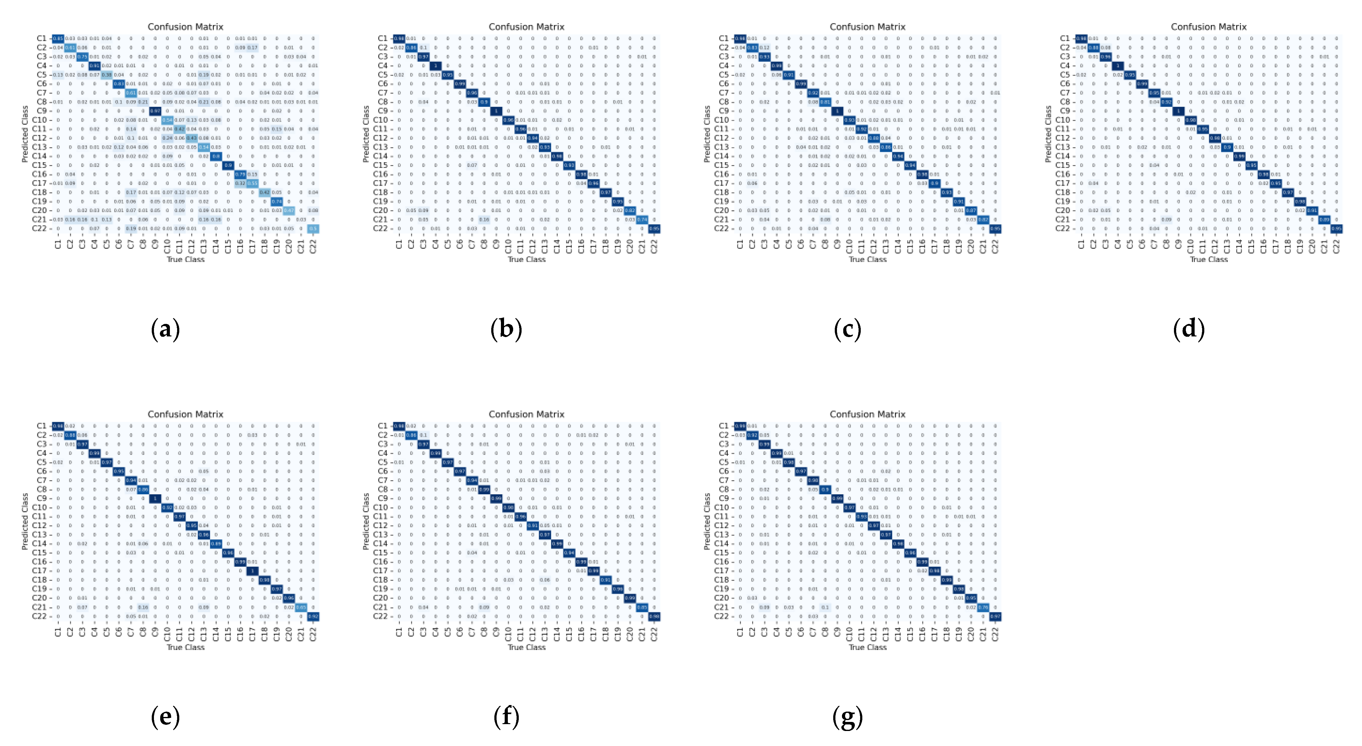
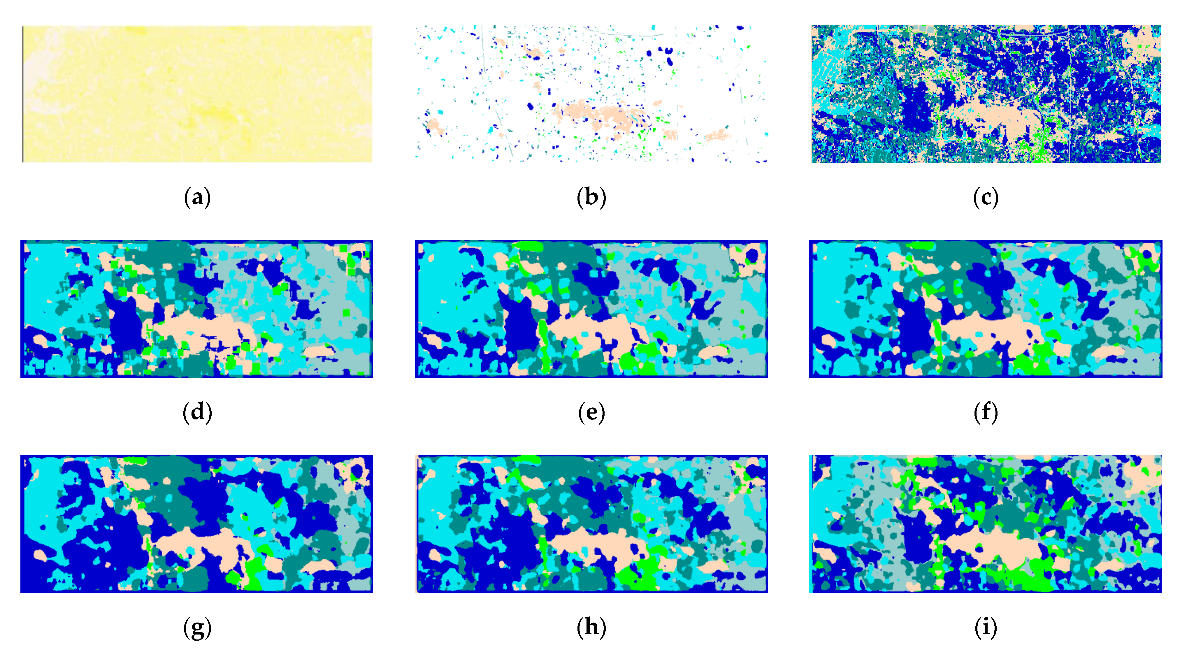
To evaluate the performance of the proposed PTCN, we first collect the classification accuracies of the competitors on the UP dataset. The classification results and training times are shown in

Table 8. Classification results and training times (TT) of the UP dataset.

Class	SVM	DBMA	DBDA	PCIA	SSGC	OSDN	PTCN
C1	87.71 ± 4.45	94.88 ± 0.74	95.89 ± 2.80	94.18 ± 1.84	97.37 ± 1.95	96.99 ± 2.16	97.90 ± 1.26
C2	89.97 ± 0.98	99.30 ± 0.16	99.10 ± 0.18	99.53 ± 0.19	99.53 ± 0.48	99.80 ± 0.04	98.53 ± 0.80
C3	75.85 ± 2.5	84.91 ± 5.01	95.76 ± 7.29	92.96 ± 4.15	74.24 ± 11.18	93.62 ± 5.47	99.04 ± 1.28
C4	93.90 ± 2.35	95.23 ± 0.54	95.30 ± 0.86	97.61 ± 0.27	99.17 ± 0.26	99.06 ± 1.19	99.75 ± 0.09
C5	97.66 ± 0.86	99.42 ± 0.12	98.72 ± 0.26	99.26 ± 0.27	99.81 ± 0.15	96.04 ± 0.65	99.37 ± 0.40
C6	88.42 ± 4.84	99.03 ± 1.14	98.70 ± 0.40	99.86 ± 0.41	99.63 ± 0.46	99.87 ± 0.07	99.42 ± 0.73
C7	77.75 ± 10.55	91.93 ± 1.73	98.40 ± 2.09	98.32 ± 1.12	99.90 ± 0.08	97.75 ± 2.07	98.34 ± 4.37
C8	75.96 ± 2.5	83.83 ± 2.23	91.24 ± 1.88	87.51 ± 4.00	96.16 ± 5.40	90.83 ± 3.05	92.94 ± 8.89
C9	99.98 ± 0.04	99.30 ± 0.25	88.52 ± 2.23	97.96 ± 0.70	96.89 ± 0.84	97.65 ± 1.42	96.60 ± 1.05
OA (%)	87.72 ± 0.68	95.98 ± 0.31	97.08 ± 0.79	97.09 ± 0.89	97.05 ± 1.02	97.96 ± 0.83	97.99 ± 1.56
AA (%)	87.47 ± 0.34	94.21 ± 0.59	95.73 ± 1.05	96.35 ± 1.08	95.86 ± 1.03	96.85 ± 1.09	97.99 ± 1.59
Kappa	0.8347 ± 0.0096	0.9465 ± 0.0041	0.9613 ± 0.0104	0.9614 ± 0.0119	0.9609 ± 0.0135	0.9730 ± 0.0110	0.9733 ± 0.0208
TT (s)	-	23.62	26.09	34.66	34.67	18.45	30.14

. The best OA, AA, Kappa, and the smallest training time are highlighted in bold. By observing the classification results, we can see that the SVM obtains the lowest OA (87.72%), which is significantly lower than that of the posterior 3D convolutional networks. It is understandable that the SVM uses only the spectral features of the HSI as the discriminative information, while the posterior 3D convolutional networks apply the spatial contextual information along with the spectral features to extract the discriminative information. The PCIA provides slightly higher OA than DBMA, DBDA, and SSGC. It shows that multi-scale convolution technology is effective in extracting discriminable features from HSI datasets. The OSDN and PTCN provide competitive classification results (97.96%, 97.99%). The PTCN achieves the highest OA among the 3D convolutional networks, which is 2.01%, 0.91%, 0.9%, 0.94%, and 0.03% higher than that of other methods. However, we can see that the standard deviation of the PTCN is relatively large, especially for C7 (4.37%) and C8 (8.89%). It indicates that although the proposed PTCN can obtain high classification accuracy, the stability (generalization) of the network is poor and the performance is influenced by the quality of the training samples. SSGC and PCIA take more time to train the model, which is discussed in Section 5.4. We select the confusion matrix of primary classification results of the UP dataset that is close to the average accuracy, which is shown in Figure 4. We can see that C3, C7, and C8 are hard to be classified for SVM. The C3 is misclassified to C1 (15%) and C8 (11%). The C7 is misclassified to C1 (20%). The C8 is misclassified to C1 (5%) and C3 (16%). For the DBMA, C3 and C8 are hard to be classified. The C3 is misclassified to C7 (2%), C8 (5%), and C9 (2%). The C8 is misclassified to C1 (2%) and C3 (15%). For the DBDA, we can see different results from DBMA. C8 and C9 are hard to be classified for DBDA. The C8 is misclassified to C3 (5%). The C9 is misclassified to C3 (2%) and C5 (4%). For the PCIA, C8 is hard to be classified. The C8 is misclassified to C3 (10%). For the SSGC, C3 is hard to be classified. The C3 is misclassified to C8 (8%). For the OSDN, C8 is hard to be classified, and the C8 is misclassified to C1 (3%) and C3 (10%). For the PTCN, the C8 is also hard to be classified, and the C8 is misclassified to C3 (10%). The full-factor classification maps of the competitors are shown in Figure 5. We can see that many salt–pepper noises appear in the classification map of SVM, which only invites spectral signatures of HSI to classify the pixels. In contrast, the classification maps of the 3D convolutional networks are smoother. The observation indicates that the classification map obtained by the 3D spectral–spatial convolutional network tends to be spatially smooth by introducing spatial contextual information when classifying the HSI datasets.

To further evaluate the performance of the PTCN, the HH dataset, which is a high spatial resolution (0.043 m per pixel) HSI dataset, is introduced to the experiment. The classification results are listed in

Table 9. Classification results and training times (TT) of the HH dataset.

Class	SVM	DBMA	DBDA	PCIA	SSGC	OSDN	PTCN
C1	86.68 ± 1.00	98.74 ± 0.13	98.31 ± 0.28	98.90 ± 0.32	97.85 ± 1.57	98.63 ± 0.24	99.19 ± 0.21
C2	57.37 ± 4.00	88.96 ± 1.33	88.13 ± 0.98	90.05 ± 1.94	88.34 ± 3.53	81.77 ± 2.30	86.50 ± 2.58
C3	76.01 ± 0.79	95.34 ± 0.39	94.28 ± 0.92	97.87 ± 1.57	96.10 ± 1.97	97.61 ± 2.14	97.42 ± 1.79
C4	91.30 ± 0.19	99.48 ± 0.07	99.37 ± 0.13	99.66 ± 0.14	99.80 ± 0.05	99.25 ± 0.24	99.41 ± 0.32
C5	37.54 ± 2.41	93.16 ± 0.78	94.64 ± 0.81	96.75 ± 1.08	91.68 ± 5.03	96.44 ± 1.74	94.68 ± 2.54
C6	82.26 ± 1.17	98.31 ± 0.47	98.32 ± 0.45	99.05 ± 0.20	98.70 ± 0.36	99.16 ± 0.15	98.38 ± 0.53
C7	62.42 ± 1.20	92.37 ± 0.92	90.63 ± 1.60	93.01 ± 1.11	94.65 ± 1.31	95.14 ± 0.95	94.72 ± 0.88
C8	28.04 ± 6.37	94.14 ± 1.12	74.46 ± 3.40	89.61 ± 2.09	65.99 ± 8.65	89.70 ± 4.44	98.57 ± 1.25
C9	96.47 ± 0.47	99.34 ± 0.13	98.01 ± 0.39	99.57 ± 0.09	99.17 ± 0.30	98.61 ± 0.34	98.90 ± 0.22
C10	54.97 ± 1.44	94.05 ± 1.24	94.52 ± 1.04	96.86 ± 0.80	93.73 ± 2.43	97.92 ± 0.91	97.26 ± 1.07
C11	52.19 ± 0.73	93.07 ± 0.73	91.89 ± 1.65	93.37 ± 1.34	91.79 ± 5.59	90.18 ± 1.59	92.37 ± 1.79
C12	44.27 ± 2.72	93.56 ± 0.64	88.16 ± 2.38	93.58 ± 2.27	83.30 ± 7.51	93.38 ± 1.92	97.84 ± 0.79
C13	54.27 ± 1.70	93.03 ± 0.62	91.05 ± 1.11	92.48 ± 3.64	93.98 ± 3.90	94.32 ± 1.07	94.71 ± 2.87
C14	80.94 ± 2.47	92.92 ± 1.68	92.72 ± 2.45	98.62 ± 0.47	97.27 ± 1.17	98.35 ± 0.83	98.26 ± 0.57
C15	68.38 ± 35.71	99.89 ± 0.18	97.69 ± 2.10	98.56 ± 0.89	98.31 ± 0.41	96.16 ± 0.69	99.33 ± 1.25
C16	79.24 ± 1.27	97.49 ± 0.64	97.88 ± 2.94	98.01 ± 0.35	98.85 ± 0.35	99.64 ± 0.23	99.49 ± 0.28
C17	51.61 ± 4.32	97.53 ± 1.67	92.79 ± 3.33	98.10 ± 1.14	97.20 ± 2.16	89.09 ± 3.08	96.00 ± 3.68
C18	44.21 ± 4.45	97.20 ± 0.80	93.73 ± 0.67	98.17 ± 0.52	97.33 ± 0.57	97.27 ± 0.50	98.32 ± 0.79
C19	70.41 ± 2.62	94.26 ± 0.49	94.47 ± 1.24	93.85 ± 1.16	92.29 ± 1.82	95.87 ± 1.13	92.67 ± 0.85
C20	51.27 ± 5.03	91.57 ± 1.26	85.71 ± 3.12	97.21 ± 0.88	98.02 ± 0.94	95.42 ± 1.50	95.86 ± 2.72
C21	5.36 ± 5.25	84.35 ± 2.49	79.13 ± 2.60	87.99 ± 2.27	70.71 ± 7.23	91.04 ± 4.72	86.42 ± 2.04
C22	51.96 ± 3.71	96.51 ± 0.54	97.04 ± 0.68	98.50 ± 0.39	97.63 ± 1.23	97.73 ± 0.36	96.71 ± 0.73
OA (%)	79.55 ± 0.14	97.05 ± 0.16	96.19 ± 0.21	97.67 ± 0.57	96.67 ± 0.56	97.51 ± 0.30	97.73 ± 0.40
AA (%)	59.87 ± 1.14	94.79 ± 0.32	92.40 ± 0.17	95.90 ± 0.73	92.85 ± 0.77	95.12 ± 0.31	96.05 ± 0.47
Kappa	0.7359 ± 0.0019	0.9626 ± 0.0021	0.9518 ± 0.0026	0.9705 ± 0.0072	0.9580 ± 0.0071	0.9685 ± 0.0038	0.9712 ± 0.0051
TT (s)	-	67.58	80.26	83.03	84.57	97.66	117.09

. Similar to the UP dataset, the SVM obtains the lowest OA (79.55%) among the competitors. Checking the classification accuracy of various categories, we can see that some categories (C5, C8, C11, C12, C18, C20, C21, and C22) are difficult to discriminate by only employing spectral signatures. The 3D spectral–spatial neural networks obtain higher classification accuracies in most categories, OA, AA, and Kappa. The experimental results demonstrate again that the accuracy of the classification methods can be improved by appropriately introducing spatial contextual information in the training process. The PCIA and PTCN achieve relatively high overall accuracies (97.67%, 97.73%). DBMA achieves the lowest training time (67.58 s). The standard deviations of the OAs of the competitors range from 0.16% to 0.57%, which indicates that the OAs of the methods are stable. It may be due to the fact that sufficient training samples (3881) can optimize the classification models adequately in the training process and thus improve the generalization of the models. The heatmap of the normalized confusion matrix, which is the closest to the average results for HH dataset, is shown in Figure 6. From the normalized confusion matrix, we can see that the C5, C8, C11, C12, C18, C20, C21, and C22 are hard to be classified for SVM. The C5 is mainly misclassified to C1 (13%), C3 (8%), C4 (%7), and C13 (19%). The C8 is mainly misclassified to C7 (9%), C10 (9%), C13 (21%), and C14 (8%). The C11 is mainly misclassified to C7 (14%) and C19 (15%). The C12 is mainly misclassified to C7 (10%) and C10 (24%). The C18 is mainly misclassified to C7 (17%) and C11 (12). The C20 is mainly misclassified to C7 (7%), C11 (9%), C13 (9%), and C22 (8%). The accuracy of the C21 is only 3% in the confusion matrix, and is mainly misclassified to C2 (16%), C3 (16%), C4 (10%), C5 (13%), C13 (16%), and C14 (16%). The C22 is mainly misclassified to C4 (7%), C7 (19%), and C11 (9%). For the DBMA, the C21 is hard to be classified, and the C21 is mainly misclassified to C8 (16%). For the DBDA, the C21 is also hard to be classified, and the C21 is mainly misclassified to C3 (4%), and C8 (8%). For the PCIA, the C21 is hard to be classified, and is mainly misclassified to C8 (9%). For the SSGC, the C8 and C21 are hard to be classified. The C8 is mainly misclassified to C7 (8%) and C13 (4%). The C21 is mainly misclassified to C3 (7%), C8 (16%), and C13 (9%). For the OSDN, the C2 is hard to be classified, and is mainly misclassified to C3 (10%). For the PTCN, the C2 and C21 are hard to be classified. The C2 is mainly misclassified to C1 (3%) and C3 (5%). The C21 is mainly misclassified to C3 (9%) and C8 (10%). From Figure 7, we can see that there are some salt-pepper noises in the classification map of SVM. The DBMA, DBMA, PCIA, SSGC, OSDN, and PTCN provide better classification maps than SVM. However, there are still some ambiguities and misclassifications in C2 and C21.

Although PTCN performs well on the UP and HH datasets, the classification accuracies are already saturated (above 96%). In those cases, margins for improvement are limited. As a result, we invite the JX dataset to further evaluate the performance of the PTCN, which is a more challenging HSI dataset. The JX dataset is a satellite dataset with mining and agriculture areas. In particular, the labeled pixels of the JX dataset are disjointly marked, which can effectively limit the ability of the 3D spectral–spatial convolutional networks to extract spatial contextual information via the cube-based method. The classification results are shown in

Table 10. Classification results and training times (TT) of the JX dataset.

Class	SVM	DBMA	DBDA	PCIA	SSGC	OSDN	PTCN
C1	74.04 ± 4.61	87.11 ± 0.75	89.99 ± 0.68	82.76 ± 1.56	85.04 ± 6.05	91.65 ± 0.91	83.17 ± 3.39
C2	14.95 ± 18.99	32.56 ± 2.23	37.91 ± 2.05	34.59 ± 11.75	53.10 ± 27.56	45.19 ± 6.39	33.01 ± 4.51
C3	48.39 ± 25.68	50.04 ± 0.83	50.14 ± 1.70	65.85 ± 3.55	49.64 ± 9.07	52.81 ± 3.21	58.96 ± 7.71
C4	26.50 ± 24.54	45.46 ± 2.63	46.89 ± 1.40	49.17 ± 3.80	49.94 ± 5.03	52.89 ± 6.17	46.72 ± 3.07
C5	55.65 ± 13.53	55.33 ± 2.47	54.65 ± 3.14	51.97 ± 2.94	53.99 ± 9.53	51.71 ± 4.21	78.10 ± 2.99
C6	17.56 ± 23.69	59.50 ± 4.54	62.22 ± 1.95	70.64 ± 2.99	72.26 ± 24.29	65.68 ± 1.84	65.18 ± 9.30
OA (%)	63.98 ± 1.64	69.70 ± 0.92	71.41 ± 0.71	72.22 ± 1.13	70.65 ± 2.56	72.33 ± 1.08	72.92 ± 1.06
AA (%)	39.68 ± 14.03	55.00 ± 1.80	56.97 ± 0.54	59.16 ± 2.94	60.67 ± 8.00	59.99 ± 2.12	60.86 ± 1.47
Kappa	0.4276 ± 0.0568	0.5474 ± 0.0099	0.5767 ± 0.0077	0.5608 ± 0.0230	0.5439 ± 0.0595	0.5931 ± 0.0116	0.5797 ± 0.0164
T (s)	-	8.76	7.31	5.77	6.19	6.73	9.01

. We can see that although the SVM provides the lowest OA, the margins with 3D convolutional networks are relatively small, ranging from 5.72% to 8.94%. It is understandable that the disjointly marked samples restrict the spatial information. Under this condition, the 3D spectral–spatial convolutional networks (spectral–spatial-based methods) provide limited improvement in classification accuracy over the SVM (spectral-based methods). The PCIA, OSDN, and PTCN provide higher OAs than the other convolutional networks. The PTCN gives competitive results in both classification accuracy and standard deviation. The heatmap of the normalized confusion matrix, which is the closest to the average results for JX dataset, is shown in Figure 8. From the confusion matrix, we can see that the C2, C3, C4, and C6 are hard to be classified for SVM. The C2 is mainly misclassified to C1 (19%), C4 (21%), and C5 (19%). The C3 is mainly misclassified to C1 (25%). The C4 is mainly misclassified to C1 (19%) and C5 (27). The C6 is mainly misclassified to C1 (23%). For the spectral–spatial 3D convolutional networks, the C2 and C4 are still hard to be classified. The C2 is mainly misclassified to C4 (21%, 20%, 20%, 17%, 17%, and 6%), and C5 (29%, 28%, 32%, 24%, 22%, and 11%) for DBMA, DBDA, PCIA, SSGC, OSDN, and PTCN. The full-factor classification maps for JX dataset are shown in Figure 9. We can see that the PTCN provides a finer-grained classification map than other convolutional networks. It is probably because we invite the polarized full attention block in the feature fusion stage, which can extract more detailed information than the former methods.

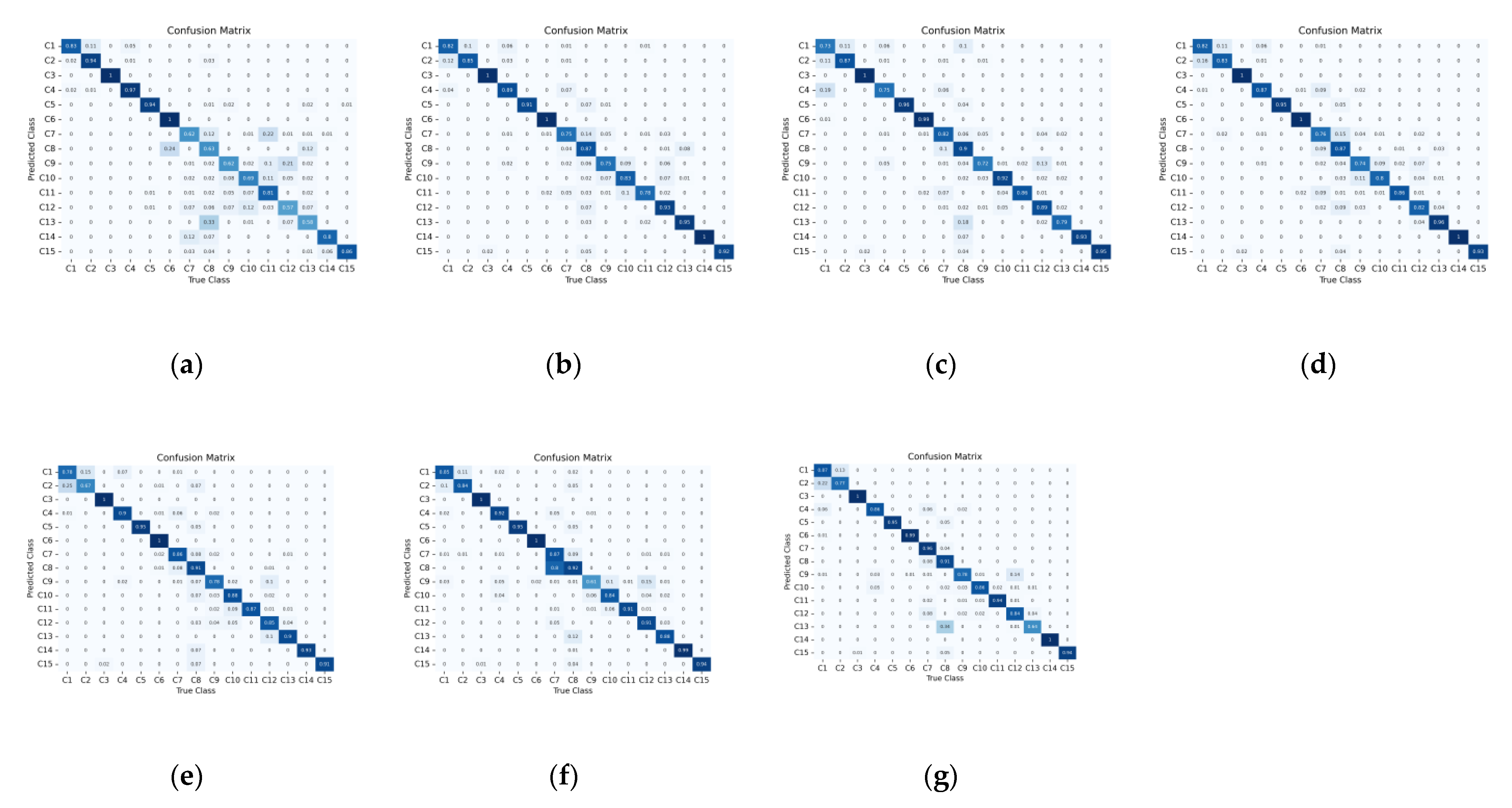
Finally, the HU dataset is implemented to investigate the effectiveness of the PTCN under small sample conditions. In the experiment, the number of training samples of different categories ranges from 3 to 12, which is difficult to adequately train the classification models. Viewing

Table 11. Classification results and training times (TT) of the HU dataset.

Class	SVM	DBMA	DBDA	PCIA	SSGC	OSDN	PTCN
C1	86.37 ± 7.64	89.61 ± 1.02	90.10 ± 0.42	90.16 ± 0.22	92.19 ± 0.82	91.81 ± 0.78	85.67 ± 2.96
C2	92.44 ± 3.90	83.66 ± 0.96	82.01 ± 1.52	85.68 ± 0.81	86.88 ± 0.77	78.60 ± 2.47	82.39 ± 0.97
C3	99.56 ± 0.16	100.00 ± 0.00	100.00 ± 0.00	100.00 ± 0.00	99.73 ± 0.20	100.00 ± 0.00	100.00 ± 0.00
C4	87.18 ± 7.04	90.21 ± 1.67	95.88 ± 0.96	95.19 ± 1.57	87.89 ± 4.94	84.74 ± 0.74	90.18 ± 2.31
C5	88.42 ± 8.45	89.41 ± 1.49	91.74 ± 0.42	84.48 ± 0.12	94.42 ± 0.41	95.02 ± 0.52	93.37 ± 1.32
C6	95.40 ± 6.45	100.00 ± 0.00	99.74 ± 0.13	99.45 ± 0.17	100.00 ± 0.00	100.00 ± 0.00	100.00 ± 0.00
C7	72.11 ± 7.12	83.57 ± 3.85	75.07 ± 2.02	74.17 ± 4.06	81.37 ± 5.37	86.36 ± 1.93	92.46 ± 1.49
C8	71.40 ± 4.73	92.74 ± 0.28	88.48 ± 5.88	84.32 ± 10.26	86.62 ± 11.17	77.32 ± 6.85	95.94 ± 2.39
C9	68.68 ± 5.75	70.17 ± 1.94	77.28 ± 3.96	83.71 ± 10.81	73.79 ± 5.21	79.38 ± 4.54	68.94 ± 6.40
C10	72.17 ± 3.78	81.47 ± 3.04	83.86 ± 3.25	73.65 ± 3.77	84.96 ± 4.11	87.02 ± 4.72	85.21 ± 0.96
C11	70.88 ± 5.48	93.19 ± 2.70	92.08 ± 4.04	93.40 ± 5.88	97.68 ± 1.43	85.49 ± 6.00	95.04 ± 2.67
C12	63.53 ± 4.42	73.70 ± 2.15	65.77 ± 3.35	71.36 ± 1.23	71.64 ± 8.85	82.63 ± 4.44	76.52 ± 5.44
C13	52.27 ± 32.33	83.96 ± 1.99	74.50 ± 10.10	64.50 ± 5.64	50.04 ± 19.61	70.72 ± 4.64	60.44 ± 5.06
C14	83.28 ± 13.44	100.00 ± 0.00	92.68 ± 0.00	100.00 ± 0.00	92.68 ± 0.00	94.89 ± 4.77	99.58 ± 0.84
C15	96.61 ± 5.17	84.18 ± 1.51	90.87 ± 0.19	89.80 ± 0.36	90.08 ± 0.89	82.12 ± 1.50	86.97 ± 1.20
OA (%)	78.90 ± 1.74	85.61 ± 0.81	84.83 ± 1.58	85.01 ± 2.75	85.35 ± 3.02	85.64 ± 2.60	86.18 ± 0.60
AA (%)	80.02 ± 3.31	87.73 ± 0.46	86.67 ± 1.21	86.67 ± 2.10	86.00 ± 3.25	86.41 ± 2.27	87.52 ± 0.28
Kappa	0.7715 ± 0.0188	0.8444 ± 0.0087	0.8360 ± 0.0171	0.8379 ± 0.0298	0.8417 ± 0.0329	0.8448 ± 0.0281	0.8506 ± 0.0065
TT (s)	-	3.79	3.49	3.60	3.56	5.22	6.25

, we can see that the SVM provides the lowest OA (79.42%). The DBDA, PCIA, and SSGC achieve higher OAs (5.41%, 5.59%, 5.93%) than SVM. The DBMA and OSDN give better OAs than DBDA (0.78%, 0.81%), PCIA (0.60%, 0.63%), and SSGC (0.26%, 0.29%). The PTCN provides higher OA than DBMA (0.57%) and OSDN (0.54%). It is understandable that the simple structure of PTCN can reduce the complexity of the network and the one-shot connection can make the PTCN easier to be trained. The special designs make the PTCN more suitable for small-sample learning tasks. The heatmap of the normalized confusion matrix, which is the closest to the average results for the HU dataset, is shown in Figure 10. It can be clearly seen that the classification accuracies of the convolutional networks are higher than that of SVM for most categories. The C9, C12, and C13 are relatively hard to be classified for the convolutional networks. The C9 is mainly misclassified to C10 (9%, 1%, 9%, 2%, 10%, and 1%) and C12 (6%, 13%, 7%, 10%, 15%, and 14%) for the convolutional networks. The C12 is mainly misclassified to C8 (7%, 2%, 9%, 3%, 0%, and 0%) for the convolutional networks. The C13 is mainly misclassified to C8 (3%, 18%, 0%, 0%, 12%, and 34%) for the convolutional networks. The full-factor classification maps for the HU dataset are collected in Figure 11. Although there are still some ambiguities and misclassifications in C9, C12, and C13, the PTCN achieves consistently competitive results in most cases.

5. Discussion

5.1. Investigation of the Proportion of Training Samples

It is an important issue to investigate the classification results of the methods under different training sample proportion conditions, which allows us to assess the effectiveness of the methods from wider perspectives. The experimental results are shown in Figure 12. Observing Figure 12a, we can see that the classification accuracies of all classification methods increase with the proportion of the training samples. The PCIA, PTCN, and OSDN obtain competitive OAs among the competitors. When the proportion of training samples is larger than 4%, the OAs of all 3D spectral–spatial convolutional networks are higher than 99%, which is already approximated to the upper limit (100%). Viewing Figure 12b, we can see similar results as the UP dataset. The OSDN, PTCN, and PCIA receive consistently competitive classification results in most cases. The OAs of all convolutional networks are higher than 99% when the training sample proportion is greater than 5%. Figure 12c presents different results from the previous two HSI datasets. With the increase in the proportion of the training samples, the OAs of the classification methods are improved significantly, which range from 11.83% to 18.36%. The PCIA, OSDN, and PTCN give better classification results than other methods. The PTCN obtained the highest OAs at 4% and 5% of the training sample proportions. The experimental results demonstrate the effectiveness of the proposed PTCN in extracting discriminable features under the condition of restricted spatial contextual information. Checking Figure 12d, we can consistently see that PCIA, PTCN, and OSDN receive better classification results. The OAs of the methods are improved significantly with the increase of the training sample proportions, especially for SVM (22.15%) and OSDN (24.94%). By comparing the classification accuracy of each classification method on different HSIs with different proportions of training samples, we can see that the proposed PTCN consistently obtains competitive classification results on all HSI datasets, which can quantitatively demonstrate the effectiveness of the PTCN.

5.2. Investigation of the Spatial Patch Sizes

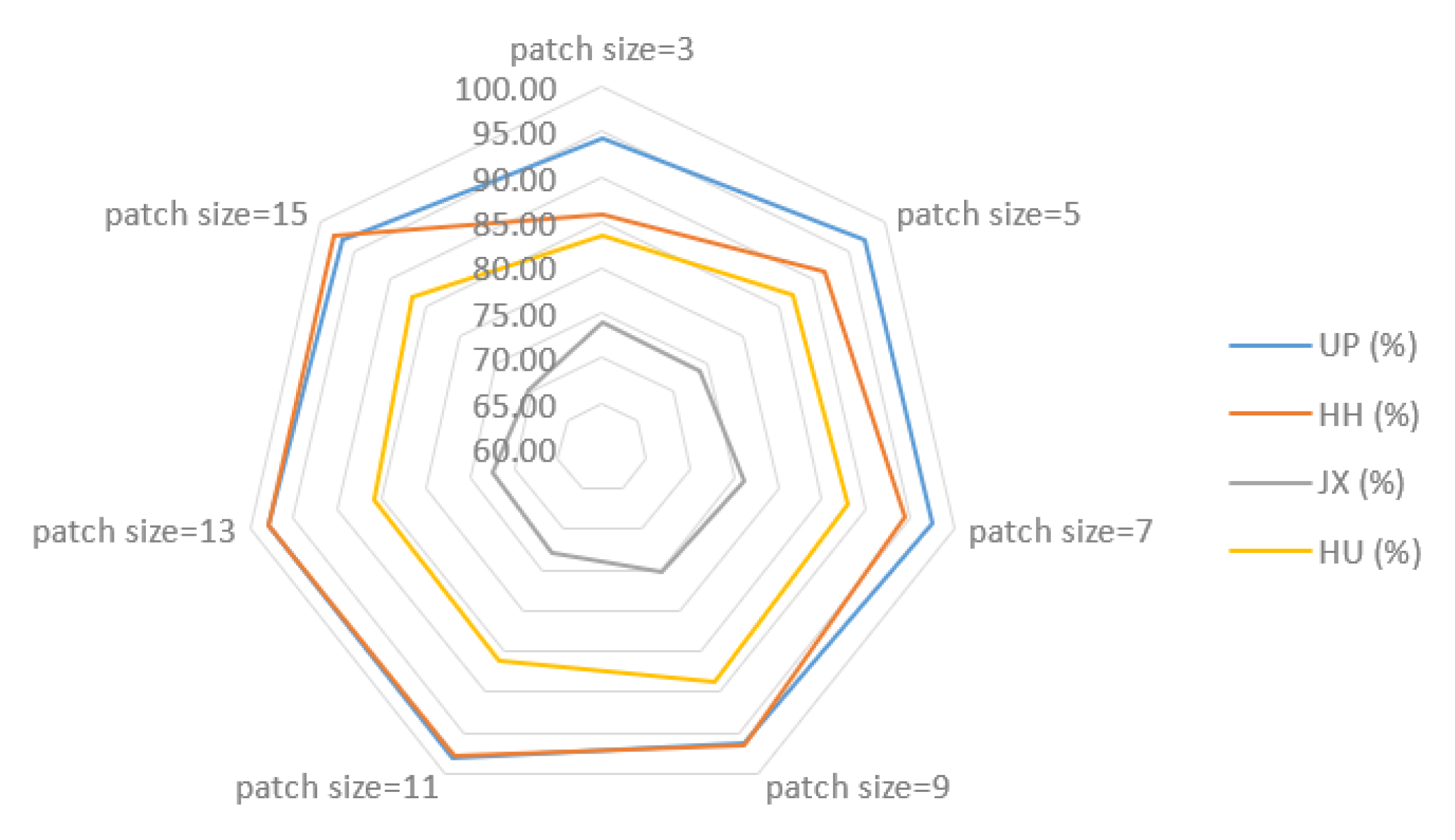
In this section, we consider the influence of spatial patch size on the classification accuracy of PTCN. In general, the cube-based classification method with a small spatial patch size can provide highly accurate spatial information and method with a large spatial patch size can provide extensive spatial information. The appropriate patch sizes can effectively improve the classification accuracies of the classification methods. The OAs of the patch sizes of PTCN on different HSIs are shown in Figure 13, which ranges from 3 to 15 in 2 intervals. We can see that the influence of the patch size is variable for the different HSI datasets. For instance, the optimal patch sizes for the UP and HH datasets are 11 and 13, while the best patch sizes for JX and HU datasets are 7 and 9. The experimental result indicates that the appropriate patch sizes are determined according to the characteristics of the HSI datasets, and it is difficult to select a patch size that is optimal for all the HSI datasets. In our experiment, we set the spatial patch size to 11 to maintain consistency.

5.3. Investigation of the Number of PCA Components

Generally speaking, abundant spectral dimensions can provide rich spectral information to discriminate pixel classes. However, highly correlated spectral dimensions with redundant spectral information can also affect classification accuracy. In this section, we check the influence of different numbers of PCA components on the proposed PTCN in the HH dataset and HU dataset and try to find an appropriate number of PCA components.

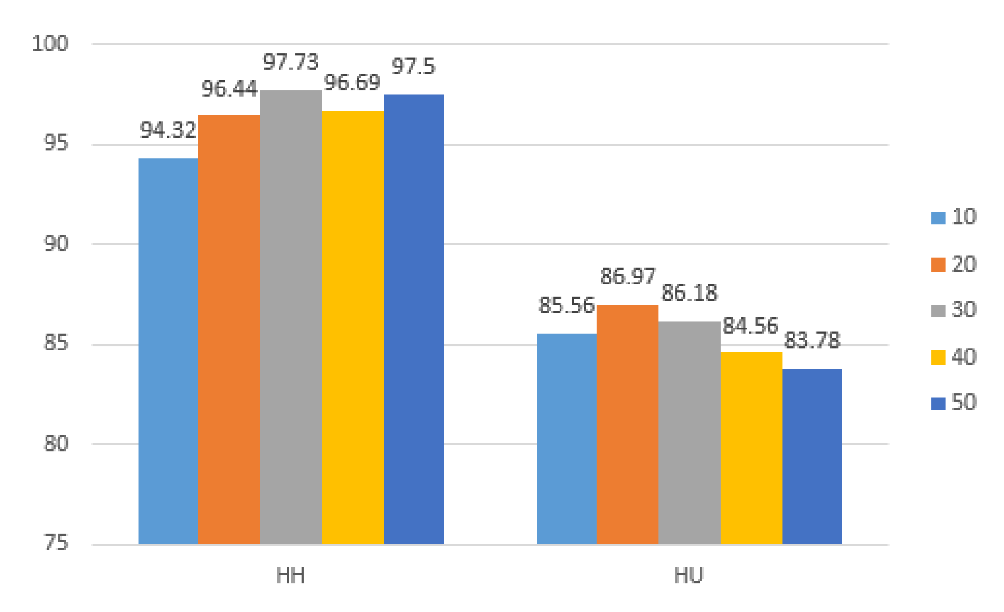
The experimental results of different numbers of PCA components of PTCN for HH and HU datasets are shown in Figure 14. We can see that the classification results are different for the HH and HU datasets. For the HH dataset, the lowest OA (94.32%) is achieved when the number of PCA components is 10. The highest OA (97.73%) is obtained when the number of PCA components is 30. When the number of PCA components is 50, the second-highest OA (97.50%) is obtained. It indicates that a certain number of spectral dimensions on the HH dataset is helpful to improve classification accuracy. However, more spectral dimensions have the potential to reduce classification accuracy. For the HU dataset, we can see that although relatively low OA (85.56%) is obtained when the number of PCA components is 10, the lowest OA (83.78%) appears when the number of PCA components is 50. The highest OA (86.97%) is achieved when the number of PCA components is 20. It indicates that providing more spectral information may lead to a decrease in classification accuracy for HU datasets. It is probably due to the Hughes phenomenon caused by the small number of training samples in the HU dataset. Comparing the classification results of the two datasets, we can see that the optimal numbers of PCA components are different for various datasets (30 for the HH dataset, 20 for the HU dataset). It is difficult to find consistent optimized parameters on multiple datasets. In our experiment, we set the number of PCA components to 30 to maintain consistency.

5.4. Ablation Analysis

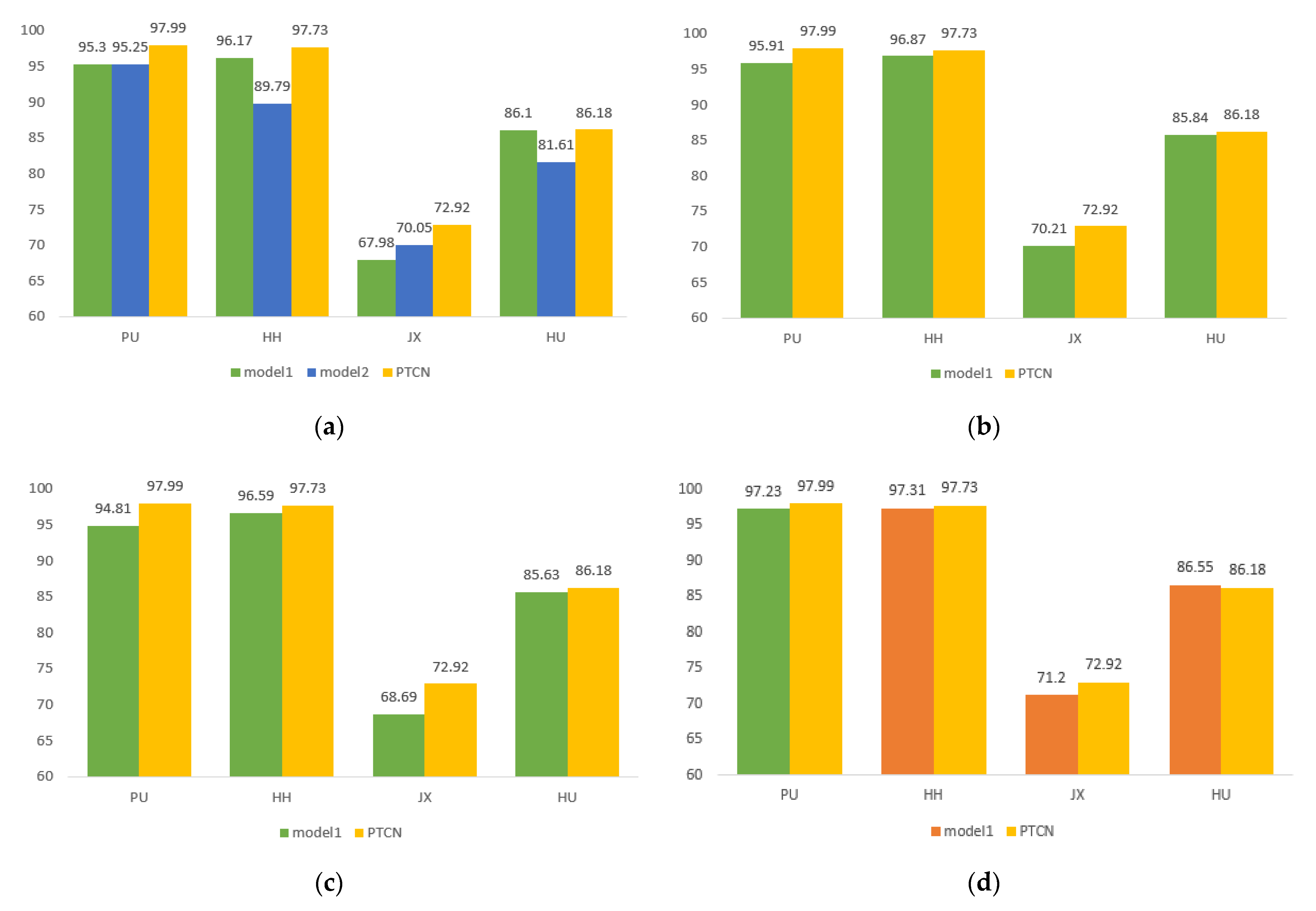
In this section, we implement ablation experiments to evaluate the effectiveness of the components of the PTCN. Four ablation experiments are designed in the experiment, including the two-branch network ablation experiment, one-shot connection ablation experiment, self-attention block ablation experiment, and FLAT-PFLAT ablation experiment. The results are shown in Figure 15. Figure 15a shows the experimental results of the two-branch network ablation experiment. Model1 denotes that only the spectral feature extraction branch network is retained in the PTCN, while model2 denotes that only the spatial feature extraction branch network is retained. We can see that the OAs of the network using either spectral or spatial feature extraction network alone are lower than that of the network using a two-branch structure (2.69%, 2.74% for the UP dataset, 1.56%, 7.94% for the HH dataset, 4.94%, 2.87% for the JX dataset, and 0.08%, 4.57% for the HU dataset). It indicates that employing both spectral and spatial feature extraction branch networks can effectively improve the performance of the convolutional network. Observing the classification results of model1 and model2, we can see that the classification accuracies of the spectral branch are higher than that of the spatial branch for the UP, HH, and HU datasets, while the classification accuracies of the spatial branch are higher than that of the spectral branch for JX dataset. It indicates that the discriminability of spectral signatures and spatial information varies among HSI datasets. In addition, it further illustrates that it is a challenging task to process highly complex HSI datasets. Figure 15b presents the effectiveness of the one-shot connection technique. The model1 indicates that the one-shot connection is not applied in the network. We can see that the classification accuracy of the PTCN is improved on all HSI datasets by employing the one-shot connection, which ranges from 0.34% to 2.71%. The results demonstrate the effectiveness of the one-shot connection technique. Figure 15c collects the OAs of the self-attention block ablation experiments. The model1 denotes that the PFLAT is not applied in the PTCN. We can clearly see that the classification accuracies of the PTCN decrease without applying the PFLAT block in the network to fusion the features (3.18%, 1.14%, 4.23%, and 0.55%). The experimental results powerfully demonstrate the effectiveness of the self-attention block and provide new thoughts for us to improve the traditional convolutional neural networks. To further evaluate the effectiveness of the PFLAT, the FLAT-PFLAT ablation experiment is implemented. The results are shown in Figure 15d. The model1 represents that the network employs the FLAT to fusion the features. We can see that the network using PFLAT has slight improvements on UP, HH, and JX datasets (0.76%, 0.42%, and 1.72%), while the accuracy decreases on the HU dataset (0.37). The classification results can prove the effectiveness of the PFLAT to some extent.

5.5. Comparison of Computational Cost and Complexity

In this section, we consider the computational cost and complexity of the convolutional networks. The number of parameters and floating-point operations (FLOPs) of the convolutional networks on the HSI datasets are listed in

Table 12. The number of parameters and FLOPs of the methods.

Dataset	Metrics	DBMA	DBDA	PCIA	SSGC	OSDN	PTCN
UP	Parameters (k)	205.31	206.11	213.38	203.06	50.16	103.02
	FLOPs (MMac)	81.28	80.79	65.45	81.31	52.31	167.15
HH	Parameters (k)	71.93	72.73	98.00	69.68	27.73	61.03
	FLOPs (MMac)	21.06	21.32	20.16	21.09	13.79	46.17
JX	Parameters (k)	234.15	234.96	260.23	231.91	55.03	112.09
	FLOPs (MMac)	94.30	93.65	75.24	94.34	60.64	193.31
HU	Parameters (k)	71.08	71.89	97.16	68.84	27.39	60.69
	FLOPs (MMac)	21.06	21.32	20.16	21.09	13.79	46.17

. We can see that the parameters of the convolutional networks vary with the structures of the networks and the input HSI datasets. In general, larger input data sizes and more output categories lead to larger parameters of the network models. Since the cube-based method is applied in the experiment, the size of the input data depends on the spatial patch size and the spectral bands of the HSI dataset. For example, the patch size of the input data is 11 for the UP dataset. The number of spectral bands is 103. The number of categories is 9. As a result, the size of the input data of the UP dataset is $103\times 11\times 11$, and the output category is 9. We can see that the OSDN and PTCN provide smaller parameters than the competitors. It is because the one-shot connection is employed in OSDN and PTCN. The parameters of PTCN are larger than that of OSDN. It is due to the fact that PTCN implements more convolutional blocks in the two-branch feature extraction network. Comparing the FLOPs of the convolutional networks, we can see that the PTCN provides the largest FLOPs, which are mainly concentrated in the spectral feature extraction branch (79.78%). However, observing Table 8, Table 9, Table 10 and Table 11, the training time of PTCN is similar to that of the other methods. It is because the early stopping technique is applied to the training process in the experiments.

6. Conclusions

In this paper, we propose a two-branch convolutional neural network with a polarized full attention mechanism for HSI classification. In the proposed PTCN, the feature extraction block is separated into two branches, the spectral branch and spatial branch. To reduce the complexity of the network and fit the small sample condition, the kernel sizes of the convolutional layers are simplified specifically for spectral and spatial feature extraction. Moreover, one-shot connection is applied in the proposed PTCN to improve the efficiency of the network to extract features in a limited training sample environment. In addition, we try to introduce the attention mechanism to solve the problem of feature fusion. We hope to use the attention mechanism to find discriminative abstract features that are worthy of attention. An improved full attention mechanism, named polarized full attention, is implemented to solve the feature fusion problem. Different from the raw full attention mechanism, the polarized full attention can provide polarizability for the network to keep high internal resolution when fuse the spectral and spatial features. Four different types of HSIs are introduced to evaluate the performance of the PTCN. Six related classification methods are employed for comparison. The experimental results show that the PTCN provides competitive performance among the competitors. In addition, the training sample proportion, the spatial patch size, the number of PCA components, the ablation analyses, and the computational cost are discussed in the experiment. In the future, we will explore the combination of convolutional networks and other self-attention mechanisms and apply the neural networks to pixel-based HSI classification tasks.

References

1. Yuan, J.W.; Wang, S.G.; Wu, C.; Xu, Y.H. Fine-Grained Classification of Urban Functional Zones and Landscape Pattern Analysis Using Hyperspectral Satellite Imagery: A Case Study of Wuhan. IEEE J. Sel. Top. Appl. Earth Obs. Remote Sens. 2022, 15, 3972–3991. [Google Scholar] [CrossRef]
2. Wei, L.F.; Wang, K.; Lu, Q.K.; Liang, Y.J.; Li, H.B.; Wang, Z.X.; Wang, R.; Cao, L.Q. Crops Fine Classification in Airborne Hyperspectral Imagery Based on Multi-Feature Fusion and Deep Learning. Remote Sens. 2021, 13, 2917. [Google Scholar] [CrossRef]
3. Peyghambari, S.; Zhang, Y. Hyperspectral remote sensing in lithological mapping, mineral exploration, and environmental geology: An updated review. J. Appl. Remote Sens. 2021, 15, 031501. [Google Scholar] [CrossRef]
4. Li, S.T.; Song, W.W.; Fang, L.Y.; Chen, Y.S.; Ghamisi, P.; Benediktsson, J.A. Deep Learning for Hyperspectral Image Classification: An Overview. IEEE Trans. Geosci. Remote Sens. 2019, 57, 6690–6709. [Google Scholar] [CrossRef]
5. Licciardi, G.; Marpu, P.R.; Chanussot, J.; Benediktsson, J.A. Linear Versus Nonlinear PCA for the Classification of Hyperspectral Data Based on the Extended Morphological Profiles. IEEE Geosci. Remote Sens. Lett. 2012, 9, 447–451. [Google Scholar] [CrossRef]
6. Villa, A.; Benediktsson, J.A.; Chanussot, J.; Jutten, C. Hyperspectral Image Classification With Independent Component Discriminant Analysis. IEEE Trans. Geosci. Remote Sens. 2011, 49, 4865–4876. [Google Scholar] [CrossRef]
7. Bandos, T.V.; Bruzzone, L.; Camps-Valls, G. Classification of Hyperspectral Images With Regularized Linear Discriminant Analysis. IEEE Trans. Geosci. Remote Sens. 2009, 47, 862–873. [Google Scholar] [CrossRef]
8. Melgani, F.; Bruzzone, L. Classification of hyperspectral remote sensing images with support vector machines. IEEE Trans. Geosci. Remote Sens. 2004, 42, 1778–1790. [Google Scholar] [CrossRef]
9. Li, J.; Bioucas-Dias, J.M.; Plaza, A. Spectral-Spatial Hyperspectral Image Segmentation Using Subspace Multinomial Logistic Regression and Markov Random Fields. IEEE Trans. Geosci. Remote Sens. 2012, 50, 809–823. [Google Scholar] [CrossRef]
10. Samat, A.; Du, P.J.; Liu, S.C.; Li, J.; Cheng, L. (ELMs)-L-2: Ensemble Extreme Learning Machines for Hyperspectral Image Classification. IEEE J. Sel. Top. Appl. Earth Obs. Remote Sens. 2014, 7, 1060–1069. [Google Scholar] [CrossRef]
11. Liu, X.B.; Hu, Q.B.; Cai, Y.M.; Cai, Z.H. Extreme Learning Machine-Based Ensemble Transfer Learning for Hyperspectral Image Classification. IEEE J. Sel. Top. Appl. Earth Obs. Remote Sens. 2020, 13, 3892–3902. [Google Scholar] [CrossRef]
12. Endo, T.; Matsumoto, M. Aurora Image Classification with Deep Metric Learning. Sensors 2022, 22, 6666. [Google Scholar] [CrossRef]
13. Kong, F.; Wen, K.; Li, Y. Regularized Multiple Sparse Bayesian Learning for Hyperspectral Target Detection. J. Geovisualization Spat. Anal. 2019, 3, 11. [Google Scholar] [CrossRef]
14. Alokasi, H.; Ahmad, M.B. Deep Learning-Based Frameworks for Semantic Segmentation of Road Scenes. Electronics 2022, 11, 1884. [Google Scholar] [CrossRef]
15. Wang, C.; Zhang, L.; Wei, W.; Zhang, Y.N. When Low Rank Representation Based Hyperspectral Imagery Classification Meets Segmented Stacked Denoising Auto-Encoder Based Spatial-Spectral Feature. Remote Sens. 2018, 10, 284. [Google Scholar] [CrossRef]
16. Chen, C.; Ma, Y.; Ren, G.B. Hyperspectral Classification Using Deep Belief Networks Based on Conjugate Gradient Update and Pixel-Centric Spectral Block Features. IEEE J. Sel. Top. Appl. Earth Obs. Remote Sens. 2020, 13, 4060–4069. [Google Scholar] [CrossRef]
17. Kumar, V.; Singh, R.S.; Dua, Y. Morphologically dilated convolutional neural network for hyperspectral image classification. Signal Process. Image Commun. 2022, 101, 116549. [Google Scholar] [CrossRef]
18. Paoletti, M.E.; Haut, J.M.; Plaza, J.; Plaza, A. Scalable recurrent neural network for hyperspectral image classification. J. Supercomput. 2020, 76, 8866–8882. [Google Scholar] [CrossRef]
19. Bai, J.; Zhang, Y.; Xiao, Z.; Ye, F.W.; Li, Y.; Alazab, M.; Jiao, L.C. Immune Evolutionary Generative Adversarial Networks for Hyperspectral Image Classification. IEEE Trans. Geosci. Remote Sens. 2022, 60, 1–14. [Google Scholar] [CrossRef]
20. Li, W.; Wu, G.D.; Zhang, F.; Du, Q.A. Hyperspectral Image Classification Using Deep Pixel-Pair Features. IEEE Trans. Geosci. Remote Sens. 2017, 55, 844–853. [Google Scholar] [CrossRef]
21. Gao, H.M.; Yang, Y.; Li, C.M.; Zhou, H.; Qu, X.Y. Joint Alternate Small Convolution and Feature Reuse for Hyperspectral Image Classification. ISPRS Int. J. Geo-Inf. 2018, 7, 349. [Google Scholar] [CrossRef]
22. Zhao, W.Z.; Du, S.H. Spectral-Spatial Feature Extraction for Hyperspectral Image Classification: A Dimension Reduction and Deep Learning Approach. IEEE Trans. Geosci. Remote Sens. 2016, 54, 4544–4554. [Google Scholar] [CrossRef]
23. Yu, C.Y.; Zhao, M.; Song, M.P.; Wang, Y.L.; Li, F.; Han, R.; Chang, C.I. Hyperspectral Image Classification Method Based on CNN Architecture Embedding with Hashing Semantic Feature. IEEE J. Sel. Top. Appl. Earth Obs. Remote Sens. 2019, 12, 1866–1881. [Google Scholar] [CrossRef]
24. Li, Y.; Zhang, H.K.; Shen, Q. Spectral-Spatial Classification of Hyperspectral Imagery with 3D Convolutional Neural Network. Remote Sens. 2017, 9, 67. [Google Scholar] [CrossRef]
25. Paoletti, M.E.; Haut, J.M.; Plaza, J.; Plaza, A. A new deep convolutional neural network for fast hyperspectral image classification. ISPRS J. Photogramm. Remote Sens. 2018, 145, 120–147. [Google Scholar] [CrossRef]
26. Roy, S.K.; Dubey, S.R.; Chatterjee, S.; Chaudhuri, B.B. FuSENet: Fused squeeze-and-excitation network for spectral-spatial hyperspectral image classification. IET Image Process. 2020, 14, 1653–1661. [Google Scholar] [CrossRef]
27. Jia, S.; Lin, Z.J.; Xu, M.; Huang, Q.; Zhou, J.; Jia, X.P.; Li, Q.Q. A Lightweight Convolutional Neural Network for Hyperspectral Image Classification. IEEE Trans. Geosci. Remote Sens. 2021, 59, 4150–4163. [Google Scholar] [CrossRef]
28. Zhang, F.; Bai, J.; Zhang, J.S.; Xiao, Z.; Pei, C.X. An Optimized Training Method for GAN-Based Hyperspectral Image Classification. IEEE Geosci. Remote Sens. Lett. 2021, 18, 1791–1795. [Google Scholar] [CrossRef]
29. Zhang, T.Y.; Shi, C.P.; Liao, D.L.; Wang, L.G. Deep Spectral Spatial Inverted Residual Network for Hyperspectral Image Classification. Remote Sens. 2021, 13, 4472. [Google Scholar] [CrossRef]
30. Dang, L.X.; Pang, P.D.; Lee, J. Depth-Wise Separable Convolution Neural Network with Residual Connection for Hyperspectral Image Classification. Remote Sens. 2020, 12, 3408. [Google Scholar] [CrossRef]
31. Zhao, J.W.; Huang, T.Y.; Zhou, Z.H. Hyperspectral image super-resolution using recursive densely convolutional neural network with spatial constraint strategy. Neural Comput. Appl. 2020, 32, 14471–14481. [Google Scholar] [CrossRef]
32. Zhao, F.; Zhang, J.J.; Meng, Z.; Liu, H.Q. Densely Connected Pyramidal Dilated Convolutional Network for Hyperspectral Image Classification. Remote Sens. 2021, 13, 3396. [Google Scholar] [CrossRef]
33. Song, W.W.; Li, S.T.; Fang, L.Y.; Lu, T. Hyperspectral Image Classification With Deep Feature Fusion Network. IEEE Trans. Geosci. Remote Sens. 2018, 56, 3173–3184. [Google Scholar] [CrossRef]
34. Paoletti, M.E.; Haut, J.M.; Fernandez-Beltran, R.; Plaza, J.; Plaza, A.J.; Pla, F. Deep Pyramidal Residual Networks for Spectral-Spatial Hyperspectral Image Classification. IEEE Trans. Geosci. Remote Sens. 2019, 57, 740–754. [Google Scholar] [CrossRef]
35. Li, R.; Zheng, S.Y.; Duan, C.X.; Yang, Y.; Wang, X.Q. Classification of Hyperspectral Image Based on Double-Branch Dual-Attention Mechanism Network. Remote Sens. 2020, 12, 582. [Google Scholar] [CrossRef]
36. Ioffe, S.; Szegedy, C. Batch Normalization: Accelerating Deep Network Training by Reducing Internal Covariate Shift. In Proceedings of the 32nd International Conference on Machine Learning (ICML), Lille, France, 6–11 July 2015. [Google Scholar]
37. Hahnloser, R.H.R.; Sarpeshkar, R.; Mahowald, M.A.; Douglas, R.J.; Seung, H.S. Digital selection and analogue amplification coexist in a cortex-inspired silicon circuit. Nature 2000, 405, 947–951. [Google Scholar] [CrossRef]
38. Khotimah, W.N.; Bennamoun, M.; Boussaid, F.; Sohel, F.; Edwards, D. A High-Performance Spectral-Spatial Residual Network for Hyperspectral Image Classification with Small Training Data. Remote Sens. 2020, 12, 3137. [Google Scholar] [CrossRef]
39. Banerjee, A.; Banik, D. Pooled hybrid-spectral for hyperspectral image classification. Multimed. Tools Appl. 2022, 1–13. [Google Scholar] [CrossRef]
40. Shi, H.; Cao, G.; Ge, Z.X.; Zhang, Y.Q.; Fu, P. Double-Branch Network with Pyramidal Convolution and Iterative Attention for Hyperspectral Image Classification. Remote Sens. 2021, 13, 1403. [Google Scholar] [CrossRef]
41. Li, Z.W.; Cui, X.S.; Wang, L.Q.; Zhang, H.; Zhu, X.; Zhang, Y.J. Spectral and Spatial Global Context Attention for Hyperspectral Image Classification. Remote Sensing 2021, 13, 771. [Google Scholar] [CrossRef]
42. Zhang, X.M.; Sun, G.Y.; Jia, X.P.; Wu, L.X.; Zhang, A.Z.; Ren, J.C.; Fu, H.; Yao, Y.J. Spectral-Spatial Self-Attention Networks for Hyperspectral Image Classification. IEEE Trans. Geosci. Remote Sens. 2022, 60, 1–15. [Google Scholar] [CrossRef]
43. Du, P.; Bai, X.; Tan, K.; Xue, Z.; Samat, A.; Xia, J.; Li, E.; Su, H.; Liu, W. Advances of Four Machine Learning Methods for Spatial Data Handling: A Review. J. Geovisualization Spat. Anal. 2020, 4, 13. [Google Scholar] [CrossRef]
44. Cao, X.H.; Li, R.J.; Wen, L.; Feng, J.; Jiao, L.C. Deep Multiple Feature Fusion for Hyperspectral Image Classification. IEEE J. Sel. Top. Appl. Earth Obs. Remote Sens. 2018, 11, 3880–3891. [Google Scholar] [CrossRef]
45. Zhang, Y.F.; Zhu, Y.L.; Hu, H.X.; Wang, H.Y. Automatic Hyperspectral Image Classification Based Ondeep Feature Fusion Network. Int. J. Robot. Autom. 2021, 36, 363–375. [Google Scholar] [CrossRef]
46. Ma, W.P.; Yang, Q.F.; Wu, Y.; Zhao, W.; Zhang, X.R. Double-Branch Multi-Attention Mechanism Network for Hyperspectral Image Classification. Remote Sens. 2019, 11, 1307. [Google Scholar] [CrossRef]
47. Li, Z.Y.; Wen, B.; Luo, Y.Z.; Li, Q.C.; Song, L.L. Hyperspectral image classification based on octave convolution and multi-scale feature fusion. Precis. Eng. -J. Int. Soc. Precis. Eng. Nanotechnol. 2022, 75, 80–94. [Google Scholar] [CrossRef]
48. Wang, M.; Zhang, X.; Niu, X.; Wang, F.; Zhang, X. Scene Classification of High-Resolution Remotely Sensed Image Based on ResNet. J. Geovisualization Spat. Anal. 2019, 3, 16. [Google Scholar] [CrossRef]
49. Zuo, X.B.; Yu, X.C.; Liu, B.; Zhang, P.Q.; Tan, X.; Wei, X.P. Graph inductive learning method for small sample classification of hyperspectral remote sensing images. Eur. J. Remote Sens. 2020, 53, 349–357. [Google Scholar] [CrossRef]
50. Wang, A.L.; Liu, C.Y.; Xue, D.; Wu, H.B.; Zhang, Y.X.; Liu, M.H. Depthwise Separable Relation Network for Small Sample Hyperspectral Image Classification. Symmetry 2021, 13, 1673. [Google Scholar] [CrossRef]
51. Pan, H.Z.; Liu, M.Q.; Ge, H.M.; Wang, L.G. One-Shot Dense Network with Polarized Attention for Hyperspectral Image Classification. Remote Sens. 2022, 14, 2265. [Google Scholar] [CrossRef]
52. Yu, L.; Xie, J.; Chen, S.C.; Zhu, L. Generating labeled samples for hyperspectral image classification using correlation of spectral bands. Front. Comput. Sci. 2016, 10, 292–301. [Google Scholar] [CrossRef]
53. Sun, C.H.; Zhang, X.H.; Meng, H.Y.; Cao, X.H.; Zhang, J.H. AC-WGAN-GP: Generating Labeled Samples for Improving Hyperspectral Image Classification with Small-Samples. Remote Sens. 2022, 14, 4910. [Google Scholar] [CrossRef]
54. Thakur, R.S.; Yadav, R.N.; Gupta, L. PReLU and edge-aware filter-based image denoiser using convolutional neural network. IET Image Process. 2020, 14, 3869–3879. [Google Scholar] [CrossRef]
55. Song, Q.; Li, J.; Li, C.; Guo, H.; Huang, R. Fully Attentional Network for Semantic Segmentation. In Proceedings of the IEEE Conference on Computer Vision and Pattern Recognition (CVPR), Nashville, TN, USA, 20–25 June 2021. [Google Scholar]
56. Yang, X.L.; Zhao, M.; Shi, S.K.; Chen, J. Deep Constrained Energy Minimization for Hyperspectral Target Detection. IEEE J. Sel. Top. Appl. Earth Obs. Remote Sens. 2022, 15, 8049–8063. [Google Scholar] [CrossRef]
57. Liu, L.X.; Qi, M.J.; Li, Y.R.; Liu, Y.J.; Liu, X.; Zhang, Z.F.; Qu, J.L. Staging of Skin Cancer Based on Hyperspectral Microscopic Imaging and Machine Learning. Biosensors 2022, 12, 790. [Google Scholar] [CrossRef]
58. He, K.; Zhang, X.; Ren, S.; Sun, J. Deep Residual Learning for Image Recognition. In Proceedings of the IEEE Conference on Computer Vision and Pattern Recognition (CVPR), Las Vegas, NV, USA, 27–30 June 2016. [Google Scholar]
59. Huang, G.; Liu, Z.; Laurens, V.; Weinberger, K.Q. Densely Connected Convolutional Networks. In Proceedings of the IEEE Conference on Computer Vision and Pattern Recognition (CVPR), Las Vegas, NV, USA, 27–30 June 2016. [Google Scholar]
60. Zhu, L.; Deng, R.; Maire, M.; Deng, Z.; Mori, G.; Tan, P. Sparsely Aggregated Convolutional Networks. In Proceedings of the European Conference on Computer Vision (ECCV), Munich, Germany, 8–14 September 2018. [Google Scholar]
61. Hu, H.; Dey, D.; Giorno, A.D.; Hebert, M.; Bagnell, J.A. Log-DenseNet: How to Sparsify a DenseNet. In Proceedings of the IEEE Conference on Computer Vision and Pattern Recognition (CVPR), Honolulu, HI, USA, 21–26 July 2017. [Google Scholar]
62. Liu, W.; Zeng, K. SparseNet: A Sparse DenseNet for Image Classification. In Proceedings of the IEEE Conference on Computer Vision and Pattern Recognition (CVPR), Salt Lake City, UT, USA, 18–23 June 2018. [Google Scholar]
63. Chao, P.; Kao, C.Y.; Ruan, Y.; Huang, C.H.; Lin, Y.L. HarDNet: A Low Memory Traffic Network. In Proceedings of the International Conference on Computer Vision (ICCV), Glasgow, UK, 23–28 August 2020. [Google Scholar]
64. Ju, R.Y.; Lin, T.Y.; Jian, J.H.; Chiang, J.S.; Yang, W.B. ThreshNet: An Efficient DenseNet Using Threshold Mechanism to Reduce Connections. IEEE Access 2022, 10, 82834–82843. [Google Scholar] [CrossRef]
65. Lee, Y.; Hwang, J.W.; Lee, S.; Bae, Y.; Park, J. An Energy and GPU-Computation Efficient Backbone Network for Real-Time Object Detection. In Proceedings of the IEEE Conference on Computer Vision and Pattern Recognition (CVPR), Long Beach, CA, USA, 15–20 June 2019. [Google Scholar]
66. Yang, Y.; Xie, Y.; Chen, X.H.; Sun, Y.B. Hyperspectral Snapshot Compressive Imaging with Non-Local Spatial-Spectral Residual Network. Remote Sens. 2021, 13, 1812. [Google Scholar] [CrossRef]
67. Xia, J.B.; Cui, Y.; Li, W.S.; Wang, L.G.; Wang, C. Lightweight Self-Attention Residual Network for Hyperspectral Classification. IEEE Geosci. Remote Sens. Lett. 2022, 19, 1–5. [Google Scholar] [CrossRef]
68. Chen, Z.T.; Tong, L.; Qian, B.; Yu, J.; Xiao, C.B. Self-Attention-Based Conditional Variational Auto-Encoder Generative Adversarial Networks for Hyperspectral Classification. Remote Sens. 2021, 13, 3316. [Google Scholar] [CrossRef]
69. Wang, G.H.; Peng, Y.Y.; Zhang, S.B.; Wang, G.; Zhang, T.; Qi, J.W.; Zheng, S.L.; Liu, Y. Pyramid self-attention mechanism-based change detection in hyperspectral imagery. J. Appl. Remote Sens. 2021, 15, 042611. [Google Scholar] [CrossRef]
70. Qing, Y.H.; Huang, Q.Z.; Feng, L.Y.; Qi, Y.Y.; Liu, W.Y. Multiscale Feature Fusion Network Incorporating 3D Self-Attention for Hyperspectral Image Classification. Remote Sens. 2022, 14, 742. [Google Scholar] [CrossRef]
71. Zhong, Y.F.; Hu, X.; Luo, C.; Wang, X.Y.; Zhao, J.; Zhang, L.P. WHU-Hi: UAV-borne hyperspectral with high spatial resolution (H-2) benchmark datasets and classifier for precise crop identification based on deep convolutional neural network with CRF. Remote Sens. Environ. 2020, 250, 112012. [Google Scholar] [CrossRef]
72. Chen, W.T.; Ouyang, S.B.; Yang, J.W.; Li, X.J.; Zhou, G.D.A.; Wang, L.Z. JAGAN: A Framework for Complex Land Cover Classification Using Gaofen-5 AHSI Images. IEEE J. Sel. Top. Appl. Earth Obs. Remote Sens. 2022, 15, 1591–1603. [Google Scholar] [CrossRef]
73. Debes, C.; Merentitis, A.; Heremans, R.; Hahn, J.; Frangiadakis, N.; van Kasteren, T.; Liao, W.Z.; Bellens, R.; Pizurica, A.; Gautama, S.; et al. Hyperspectral and LiDAR Data Fusion: Outcome of the 2013 GRSS Data Fusion Contest. IEEE J. Sel. Top. Appl. Earth Obs. Remote Sens. 2014, 7, 2405–2418. [Google Scholar] [CrossRef]
74. Zhang, S.Y.; Xu, M.; Zhou, J.; Jia, S. Unsupervised Spatial-Spectral CNN-Based Feature Learning for Hyperspectral Image Classification. IEEE Trans. Geosci. Remote Sens. 2022, 60, 1–17. [Google Scholar] [CrossRef]
Figure 1. The illustration of the residual connection, dense connection, and one-shot connection: (a) residual connection. (b) dense connection. (c) one-shot connection.
Remotesensing 15 00848 g001
Figure 2. The details of the fully attentional block. In the implementation, H × W represents the spatial size of the input feature map, and H equals W . S represents the dimension after the merge operator for a clear illustration, and S equals H and W . (a) The workflow of the fully attentional block. (b) The workflow of the construction block.
Remotesensing 15 00848 g002
Figure 3. The structure of the proposed network. (a) The workflow of the PTCN. (b) The workflow of the PFLA.
Remotesensing 15 00848 g003aRemotesensing 15 00848 g003b
Figure 4. The heatmap of normalized confusion matrix for the UP dataset. (a) SVM. (b) DBMA. (c) DBDA. (d) PCIA. (e) SSGC. (f) OSDN. (g) PTCN.
Remotesensing 15 00848 g004
Figure 5. The full-factor classification maps for the UP dataset. (a) False-color map. (b) Ground-truth map. (c) SVM. (d) DBMA. (e) DBDA. (f) PCIA. (g) SSGC. (h) OSDN. (i) PTCN.
Remotesensing 15 00848 g005
Figure 6. The heatmap of normalized confusion matrix for the HH dataset. (a) SVM. (b) DBMA. (c) DBDA. (d) PCIA. (e) SSGC. (f) OSDN. (g) PTCN.
Remotesensing 15 00848 g006
Figure 7. The full-factor classification maps for the HH dataset. (a) False-color map. (b) Ground-truth map. (c) SVM. (d) DBMA. (e) DBDA. (f) PCIA. (g) SSGC. (h) OSDN. (i) PTCN.
Remotesensing 15 00848 g007
Figure 8. The heatmap of normalized confusion matrix for the JX dataset. (a) SVM. (b) DBMA. (c) DBDA. (d) PCIA. (e) SSGC. (f) OSDN. (g) PTCN.
Remotesensing 15 00848 g008
Figure 9. The full-factor classification maps for the JX dataset. (a) False-color map. (b) Ground-truth map. (c) SVM. (d) DBMA. (e) DBDA. (f) PCIA. (g) SSGC. (h) OSDN. (i) PTCN.
Remotesensing 15 00848 g009
Figure 10. The heatmap of normalized confusion matrix for the HU dataset. (a) SVM. (b) DBMA. (c) DBDA. (d) PCIA. (e) SSGC. (f) OSDN. (g) PTCN.
Remotesensing 15 00848 g010
Figure 11. The full-factor classification maps for the HU dataset. (a) False-color map. (b) Ground-truth map. (c) SVM. (d) DBMA. (e) DBDA. (f) PCIA. (g) SSGC. (h) OSDN. (i) PTCN.
Remotesensing 15 00848 g011aRemotesensing 15 00848 g011b
Figure 12. The OAs of the methods under different training sample proportions. (a) UP. (b) HH. (c) JX. (d) HU.
Remotesensing 15 00848 g012aRemotesensing 15 00848 g012b
Figure 13. The investigation of the spatial patch sizes of the PTCN.
Remotesensing 15 00848 g013
Figure 14. The investigation of the number of PCA components of the PTCN.
Remotesensing 15 00848 g014
Figure 15. The ablation experiments of PTCN on HSI datasets. (a) Ablation experiment for two-branch network. (b) Ablation experiment for one-shot connection. (c) Ablation experiment for self-attention block. (d) Ablation experiment for FLAT and PFLAT.
Remotesensing 15 00848 g015