1. Introduction
The Digital Architecture Research Center of the National Institute of Advanced Industrial Science and Technology (AIST) conducts research using big data of geographic observations provided by various organizations. Some of the geographic observation data provided were observed by Pi-SAR2.
Pi-SAR2 is an X-band airborne polarimetric synthetic aperture radar (SAR) operated by the National Institute of Information and Communications Technology (NICT) as the successor to Pi-SAR. The greatest advantage of Pi-SAR2 is its high resolution, with a spatial resolution of up to 0.3 m (both azimuth and slant range), comparable to that of optical high-resolution satellites. In addition to its full polarimetric capability, Pi-SAR2 can simultaneously observe data for cross-track and along-track interferometry using its multiple antennas [
1,
2,
3]. These features are expected to be used for a variety of applications and research. On the other hand, the Pi-SAR2 observation data are very large due to its high resolution and require sufficient computational resources to handle.
The AIST has received approximately 400 TB of the Pi-SAR2 polarimetric observation data through a joint research project with the NICT. The Pi-SAR2 observation data are very valuable because of its high resolution, but it cannot be used effectively because the data are not well calibrated with respect to elevation. Therefore, we performed elevation calibration by utilizing the huge computational resources of the AIST. The AI Bridging Cloud Infrastructure (ABCI) is the world’s largest computational infrastructure for artificial intelligence (AI) processing, constructed and operated by the AIST. The ABCI system consists of 120 compute nodes (A) with 960 NVIDIA A100 GPU accelerators, 1088 compute nodes (V) with 4352 NVIDIA V100 GPU accelerators, a shared file system with a combined capacity of approximately 35 PB, cloud storage, and a high-speed InfiniBand network to interconnect these nodes [
4]. The ABCI makes it possible for us to process a large amount of Pi-SAR2 observation data.
In this study, we calibrated the Pi-SAR2 observational data utilizing sufficient computational resources of the ABCI. In addition, we have verified the results of calibration and created data that is intuitively easy to understand visually and can be used for deep learning and other purposes by performing scattering power decomposition. The original observation data were recorded with distortion depending on the elevation, because it was observed obliquely from an aircraft, making it difficult to link with other geographic information. Therefore, we have also corrected this by orthorectification. The contribution of this study is that we have made it possible to provide high-resolution polarimetric observation data in an easy-to-use format by organizing and solving their associated problems. In this paper, we report on the calibration, scattering power decomposition, and orthorectification of the Pi-SAR2 observation data using the ABCI.
2. Process Overview
2.1. About the Pi-SAR2 Polarimetric Observation Data Files
Pi-SAR2 has two antenna pods containing multiple antennas mounted on the bottom of the aircraft for observation. The main antenna pod has transmitting and receiving waveguide slot antennas for horizontal (H) and vertical (V) polarization. The sub antenna pod has one V-polarized receiving antenna for cross-track interferometry (CTI) and two V-polarized receiving antennas for along-track interferometry (ATI). These antennas allow full-polarimetric and interferometric observations in a single flight. The observation data are expressed in the format XYz, where X is the transmitting polarization (H or V), Y is the receiving polarization (H or V), and z is the antenna type (m: main antenna, s: sub antenna for CTI, a/f: sub antenna for ATI).
There are two types of observation data files provided by the NICT: SSC and MGP. SSC stands for Single-look Slant-range Complex and its files are created by image compressing process from the level 0 data set. It separates files for each of the observed polarizations. Its coordinate system is azimuth × slant range, and the data format is complex numbers with a real part of 4 bytes and an imaginary part of 4 bytes. MGP stands for Multi-look Ground-range Polarimetry and its files are created from the SSC files after polarimetry processing. Its coordinate system is azimuth × ground range, and data format is 8 bytes complex numbers such as SSC, but the phase reference is aligned to HHm. Only the four polarizations observed by the main antenna are provided. Although the name includes “multi-look”, all actual data has a look number of one.
Pi-SAR2 repeats multiple SAR observations while flying straight according to the observation plan after takeoff with antennas and recording equipment mounted on the aircraft. Here, a series of observations from takeoff to landing is called a “series” and each linear flight is called a “path”. The observation series is identified by the observation date, and the observation paths are numbered. The observation paths are divided into areas corresponding to 6 km in azimuth and 6 km in ground range during the process of creating the SSC files. These divided areas are called “scenes” and are numbered consecutively. The observation data provided by the NICT were observed from 22 December 2009 to 16 November 2017, and include 9324 scenes of 781 paths in 51 series, approximately 240 TB of SSC files and 160 TB of MGP files.
Most of the observation data is observed in Mode 1, which has the highest resolution. Mode 1 has a spatial resolution of 0.3 m in both range and azimuth. The pixel spacing of the MGP data is 0.25 m, and the number of pixels per scene is 24,000 × 24,000 in Mode 1. The file size is approximately 4.3 GB per polarization file. On the other hand, the SSC data has the same number of pixels in the azimuth direction as the MGP data, but the number of pixels in the range direction depends on the angle of incidence.
In this calibration and scattering power decomposition, we use the MGP data as the processing target. However, since the MGP data do not include the data observed by the sub antennas, SSC data are also used for some calculation of the calibration parameters. The processing will be done on a scene-by-scene basis.
2.2. Process Flow
Figure 1 shows a flow diagram of the process. The calibration is performed in two stages. First, we correct elevation-dependent phase rotation based on the elevation calculated by CTI to remove interferometric component caused by the antenna configuration of Pi-SAR2. The corrected data are called MGP_H. Next, we perform polarimetric calibration on the MGP_H data, and the resulting calibrated data are called MGP_C. The calibrated data are then processed in scattering power decomposition using two algorithms, respectively. Finally, the calibrated MGP_C data and the scattering power decomposition images are orthorectified based on the digital elevation model (DEM) of Geospatial Information Authority of Japan (GSI) [
5] so that they can be superimposed on the map. The details of each process are described in
Section 3,
Section 4,
Section 5 and
Section 6.
3. Elevation Correction
Pi-SAR2 uses separate antennas for H and V polarization observations. The distance between the antenna centers is 0.2 m, which causes a phase difference due to the path difference.
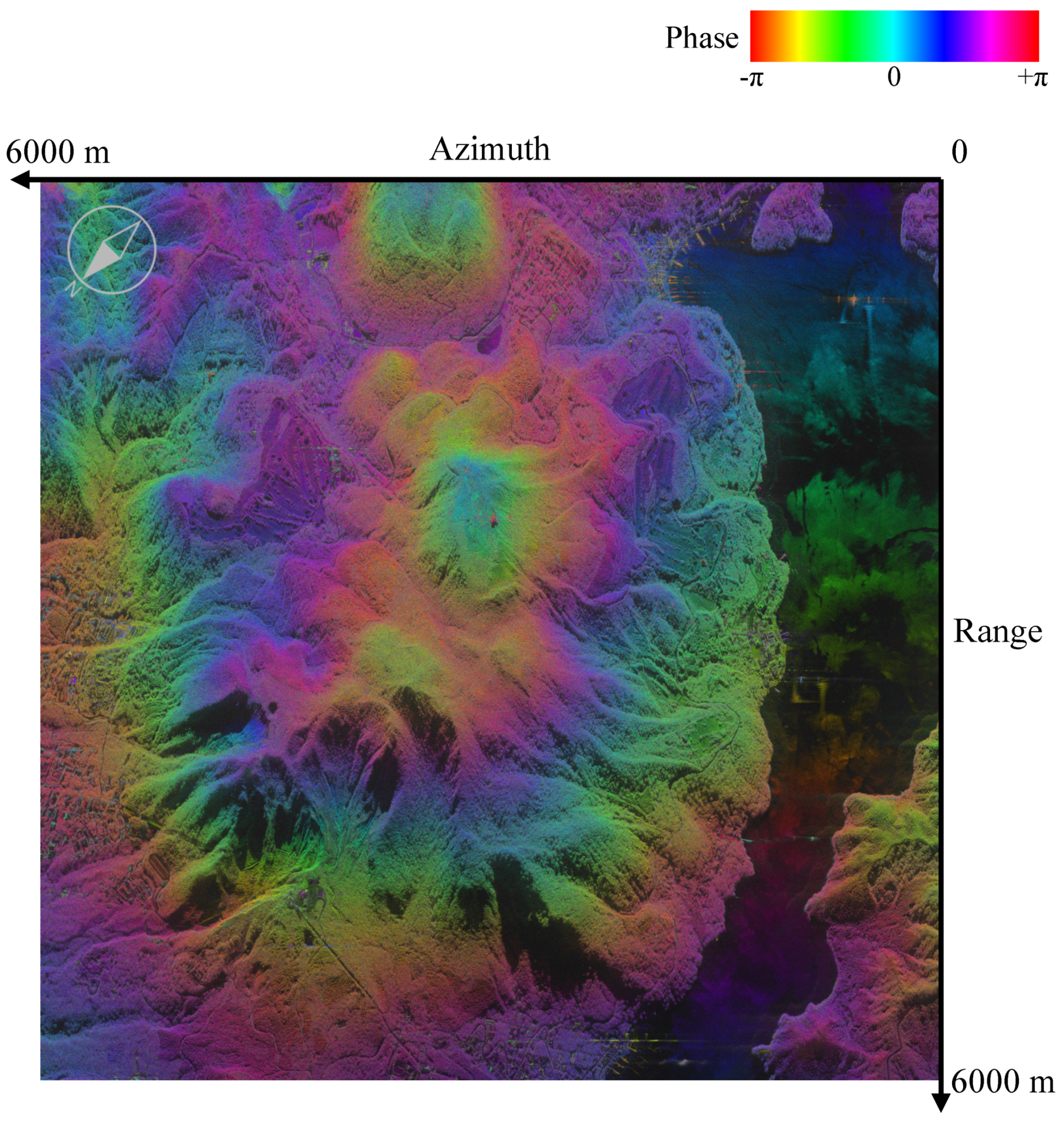
Figure 2 shows the MGP image of the VV polarization around Mount Hakone. The highest peak of Mount Hakone, Mount Kami, is shown on the center of the image, and Lake Ashi is shown on the right. The horizontal direction of the image corresponds to the Azimuth direction, with Early on the right and Late on the left. The vertical direction corresponds to the Range direction, with Near at the top and Far at the bottom. The brightness of each pixel indicates the amplitude of the signal, and the hue indicates the phase. Since the phase of the MGP images is normalized with respect to the HH polarization, the phase shown in this image represents the phase difference between the VV and HH polarizations. One can observe the phase rotation correlated with the elevation of mountains. Since Pi-SAR2 is performing CTI observations at the same time as full polarimetry observations, we correct the phase rotation using the CTI data [
6].
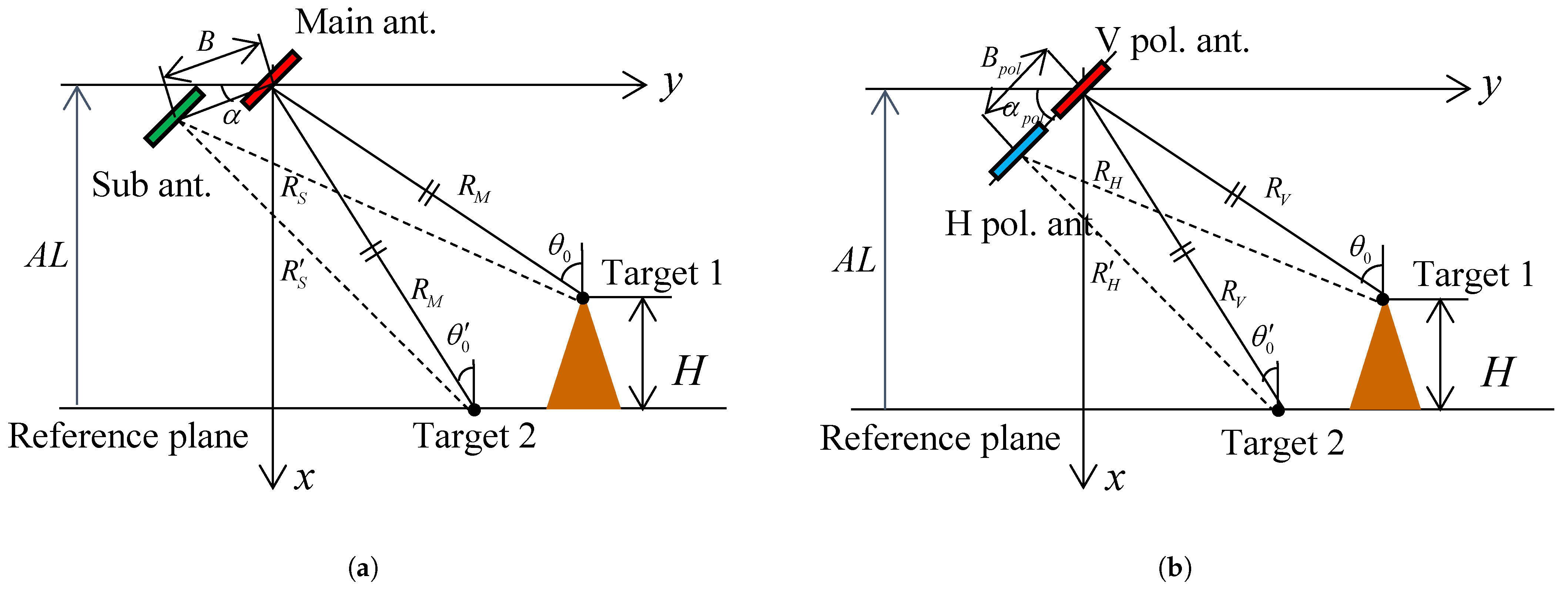
Figure 3a shows a schematic diagram of the observation of the main and sub antennas of Pi-SAR2. When
and
denote the distance between each antenna and Target 1 at an elevation
H,
can be written as the following equation,
where
B is the baseline length between the two antennas,
is the inclination of the aircraft, and
is the angle of incidence. Furthermore, when
denotes the wavelength, the phase difference
is written as the following equation,
Furthermore, when Target 2 is a point on the reference plane where the distance
from the main antenna is the same, the angle of incidence is
, and the distance from Target 2 to the sub antenna is
, and the following equation is similarly obtained.
As a result, the interferometric phase difference after removing the flat earth phase
is written as follows,
Since
, we can approximate
and
to write as follows,
Figure 3b shows a schematic diagram of the observations with the H- and V-polarized antennas in the main antenna pod. The phase difference between the H- and V-polarized antennas after removing the flat earth phase
is similarly written as follows,
where
is the distance between the centers of the H- and V-polarized antennas and
is the inclination of the antenna.
From Equations (6) and (7), the compensation formula is written as follows,
Since this formula represents a one-way component, it is subtracted as is for HV and VH polarization and doubled and subtracted for VV polarization.
In the actual processing, since the observation data of the sub antennas is only provided in the SSC files, the correction values are calculated from the interferometry of SSC_VVm and SSC_VVs files. Since the values of
and
for each observation were not available, we used fixed values for them. Interferometry is processed in 4 × 4 looks. The phase after interferometry is wrapped into
range, so the phase unwrapping process is necessary. We use the minimum Lp-norm phase unwrapping algorithm [
7]. The compensation phase is calculated based on the CTI phase after unwrapping, converted to the ground range, and then interpolated to the original resolution and applied.
Figure 4 shows the result of elevation correction of the data shown in
Figure 2. In
Figure 4, the phase rotation correlated with elevation is no longer seen. This indicates that the data has been corrected for elevation.
4. Polarimetric Calibration
When the measured scattering matrix after elevation correction is
and the true scattering matrix is
, the relation can be written as follows,
where
A is the gain,
and
are the error matrices in the receive/transmit system,
is the system noise,
and
are the H/V polarization imbalance of the receive/transmit system, and
and
are cross-talk. We assume that the system noise
has already been sufficiently eliminated in the provided data and set
for the sake of simplicity. We perform polarimetric calibration by estimating the error matrices
and
. When we define
as the post-calibration scattering matrix to obtain, we calibrate it by using the following equation,
Crosstalk
was calculated from the covariance of the scattering matrix based on Quegan’s method [
8]. However, since the magnitude of the calculated
was very small, about −32 dB, we considered them to be zero. As a result, the following equation is obtained.
There are two methods for estimating imbalance: one using corner reflectors (CRs) and the other using natural terrain such as sea, rice fields, etc. Some of the Pi-SAR2 observations were made with CRs in place. However, this is a small percentage of the total measurements, and the observation dates are also biased. Therefore, we estimate the imbalance by decomposing it into amplitude and phase. Since the amplitude of imbalance
does not vary much from one observation series to another, we calculate a single value from the observation data with CRs and apply it to all scenes. On the other hand, the imbalance phase
is directly calculated from each observation scene data using the natural terrain, because it is affected by the attachment and removal of antennas from the aircraft in each observation series. The phase of the transmit/receive imbalance ratio
is also calculated from each scene data as
, using Quegan’s method [
8].
In some observation series, CRs were placed on the beach near Niigata University, and
Figure 5 shows a scattering power decomposition image of Obs.10 on 21 August 2014, which is one of the observations with CRs. The three bright spots indicated by the arrows are the scattering by CRs. The difference in color is due to the orientation of CRs. We obtained the calibration values from the ratio of the scattering intensities for each polarization at the CR positions for the four-observation data with CRs: Obs.13 on 25 August 2013, Obs.05 on 17 October 2013, Obs.10 on 21 August 2014, and Obs.07 on 3 March 2015. The calculated ratio of scattering intensities VV/HH averaged 1.4045 with a minimum value of 1.3611 and a maximum value of 1.4873. Therefore, we set the imbalance amplitude
. Since there was no significant difference in the scattering intensity at the CR positions between HV and VH polarizations,
are used.
The following equality holds for natural targets,
Therefore, the phase of imbalance
can be written as the following equation,
We set the averaging window size to 40 pixels and the slide size to 20 pixels.
The
is calculated from the following equation based on Quegan’s method.
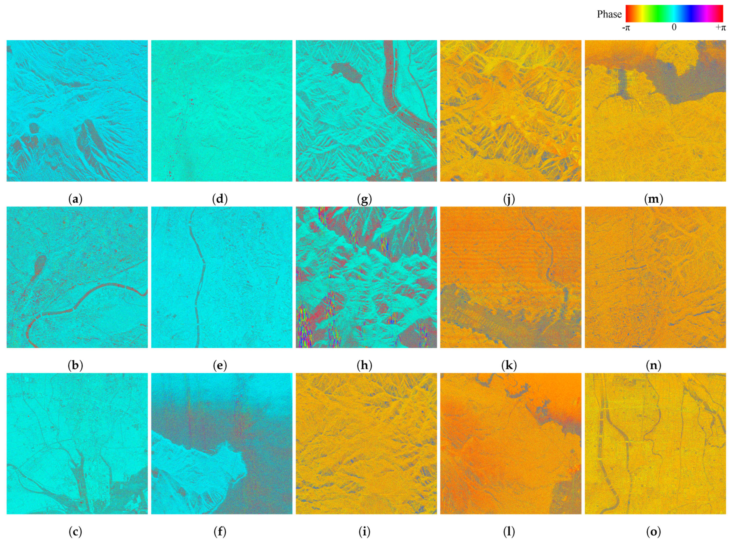
Figure 6 shows HV and VH polarization images and their phase difference
. The HV-VH phase difference is almost constant in the image except for areas with low scattering intensity such as water surface and mountain shadow. Therefore, the following equation, which is averaged over the entire scene, is used.
Figure 7 shows the HV-VH phase difference calculated for observation scenes from each observation series, along with the observation date. The phase difference was near zero for observations prior to October 2013, while it was near
for observations after August 2014. This might be attributed to a repair of the H transmitter before the observation on August 2014 [
9]. It was also found that the difference in HV-VH phase difference between different observation series was larger than between different scenes within the same observation series. This may be due to the influence of the attachment and removal of antennas from the aircraft in each observation series.
We calibrated the MGP_H data using the calculated
,
,
and
.
Figure 8 shows the VV polarization image after calibration, where the range phase rotation seen in
Figure 4 is removed and the overall phase is aligned around 0.
5. Scattering Power Decomposition
The calibrated observation data are processed by scattering power decomposition based on the scattering model. Scattering power decomposition has the advantage of being easy to understand because color images corresponding to the scattering mechanism can be obtained. In deep learning, the scattering power decomposition data is input instead of the observation data as it may have the advantage of improving the performance, due to greater focus on the scattering mechanism. In addition, since the scattering power decomposition is not performed correctly with the insufficiently calibrated observation data, we used it as a benchmark to evaluate the calibration.
There are several algorithms for scattering power decomposition. In this paper we use two algorithms, G4U [
10] and 6SD [
11]. The G4U algorithm decomposes into four components: surface scattering
, double bounce scattering
, volume scattering
, and helix scattering
. The 6SD algorithm decomposes into six components: the same four components as the G4U, oriented dipole power
and composite compound dipole power
. When creating images, the scattering power components are assigned to each RGB component as follows.
It is known that scattering power decomposition images tend to be green in areas with vegetation because of the dominance of volume scattering, and purple in areas with vertical planes such as buildings because surface scattering and double bounce scattering are stronger. Therefore, the scattering power decomposition images allow us to evaluate whether the calibration has been performed correctly.
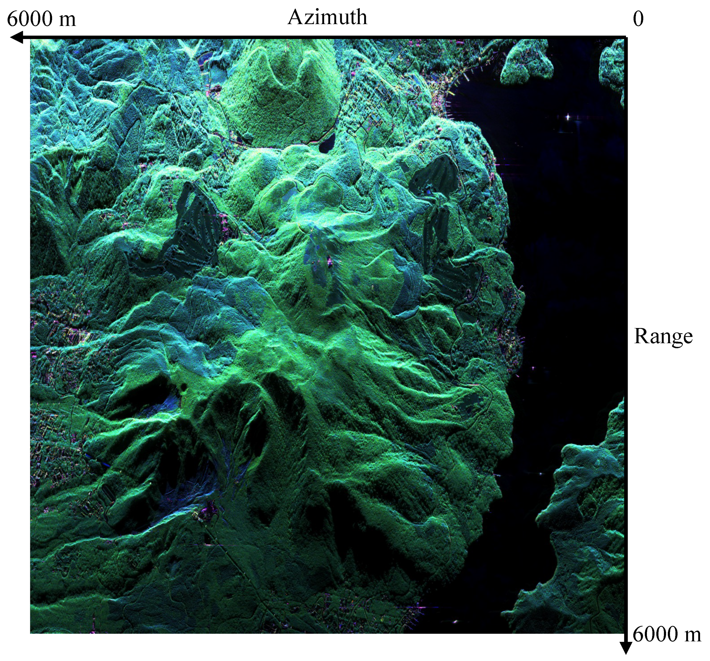
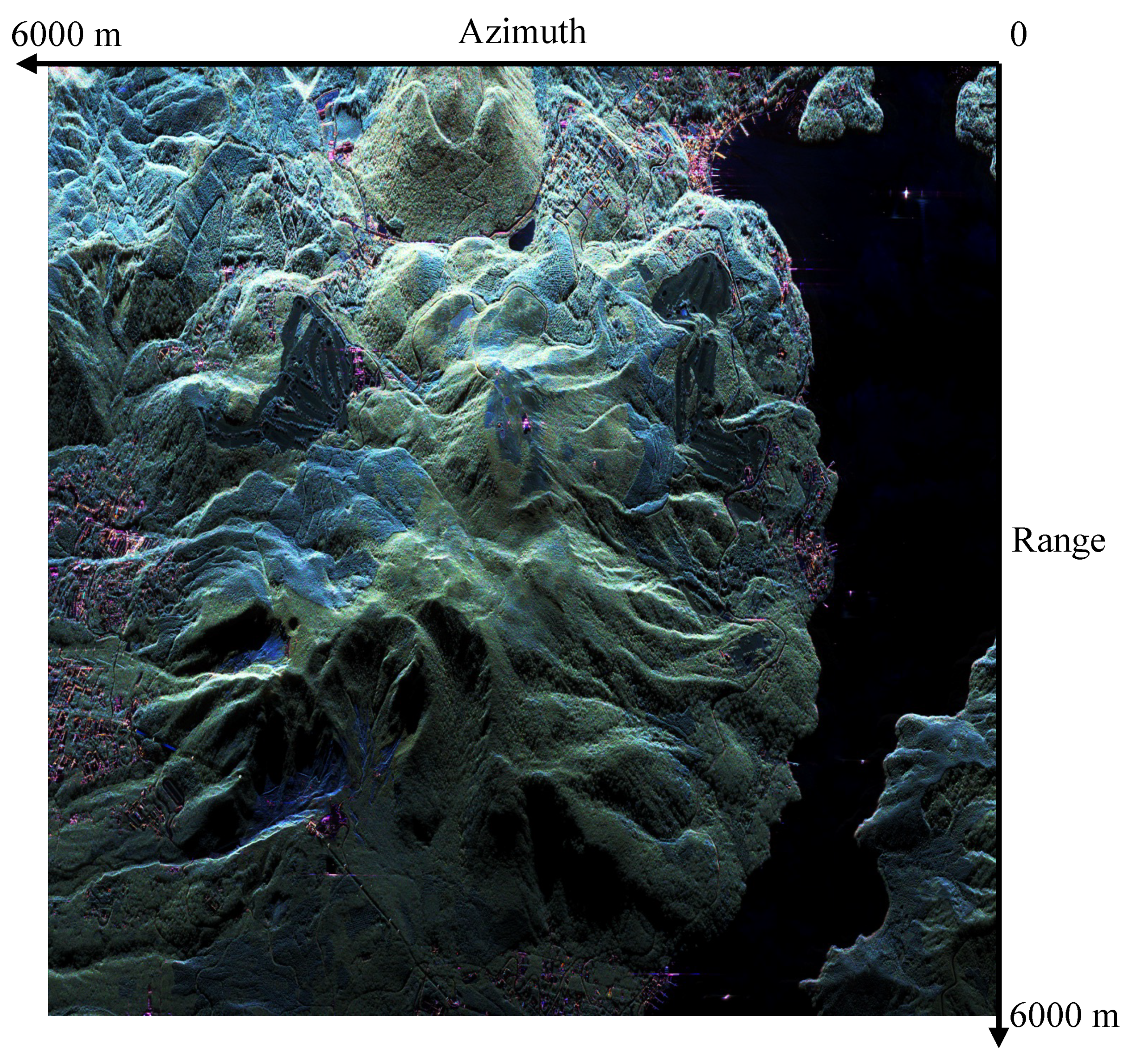
Figure 9 and
Figure 10 show results of the G4U scattering power decomposition of the observation data before and after calibration. The look size of each image is 9 × 9. The pre-calibration image shows a color band correlated with the elevation, as seen in
Figure 2, and the overall color is different from what is expected. On the other hand, the post-calibration image shows that the effect of elevation has been removed and the forested areas occupying a large part of the images are green, as expected.
Figure 11 and
Figure 12 show results of the 6SD scattering power decomposition of the observation data before and after calibration. The same trend as G4U can be seen in the pre- and post-calibration images. In addition, we show calibration results for data with different observation periods and geographical conditions.
Figure 13,
Figure 14,
Figure 15 and
Figure 16 show results of the G4U and 6SD scattering power decomposition for another area before and after calibration near Niigata University. In contrast to the mountainous area of
Figure 13,
Figure 14,
Figure 15 and
Figure 16, this area is almost flat. The square-divided areas that occupy most of the upper two-thirds of the images are cropland (mainly rice paddies), while the lower third of the images is urban area. Note that the rice paddies are flooded in August, which is when this data was observed. The effect of the elevation correction is small because of the flatness of the area, and the effect of the polarimetric calibration for HV and VH polarization is also small because this data, observed in 2013, and
, is near zero. As a result, changes between the pre- and post-calibration of this observation are smaller than those shown in
Figure 9,
Figure 10,
Figure 11 and
Figure 12. Nevertheless, improvements of the post-calibration images can be seen in the reduction of red areas, indicating double bounce scattering, which are seen in some areas of the cropland in the pre-calibration images.
6. Orthorectification
The ground range data we have handled so far are simple projections of slant range data onto a reference plane. As a result, objects with elevation from the reference plane are observed at different points than where they should be.
Figure 17 shows a schematic diagram of the position shift due to elevation. When the slant range distance of Target 1 at elevation
H is
, the scattering by Target 1 is observed as existing at Target 2, which has the same slant range distance and is closer to the antenna on the reference plane, because the radar cannot distinguish the direction of the arrival of the signal. Since this situation causes discrepancies when superimposed on maps, we orthorectify the data to make it easier to link with other geographic information systems (GIS). We use DEM10B provided by the GSI as the elevation data for the correction. DEM10B is a 10 m mesh DEM created from the contour lines on a topographic map [
5].
When the ground range distances of Target 1 and Target 2 are
and
, the relational equation is as follows,
Therefore, the position can be corrected from the elevation by the following equation,
Figure 18 shows the elevation read from the GSI DEM and
Figure 19 shows the orthorectified MGP_C_VVm image of the same data as
Figure 8. However, the origin is different from that in
Figure 8. The black areas at the top and bottom of the image are areas where data do not exist due to deformation. The high elevation region in the center of the image has moved more significantly in the far side compared to the mountain foot on the left edge of the image.
7. Process Execution
We applied calibration, scattering power decomposition, and orthorectification process to the large amount of Pi-SAR2 observation data, utilizing the sufficient computational resources of the ABCI. While there are a total of 9324 scenes of Pi-SAR2 MGP observation data provided by the NICT, we excluded scenes that were not observed in CTI mode, because they could not be corrected for elevation by CTI, and also excluded some scenes with incomplete files, and processed the remaining 7266 scenes.
While each process is implemented as a single-threaded, we used GNU Parallels to calculate multiple scenes in parallel. We chose the ABCI compute nodes to use according to the memory consumption of each process and decided the number of parallel depending on the number of its CPU cores.
Table 1 shows the coding languages, the ABCI resource type, the number of parallels per node and the processing time per scene at each stage of processing. rt_C indicates the Compute Node (V) using CPU only and rt_M indicates the Memory-intensive Node in the resource type column. Please refer to the ABCI User Guide [
12] for details on each resource type. The processing time per scene is estimated by running the process on a subset of the observed data. The interferometry stage took most of the processing time, with most of the time spent on phase unwrapping. The processing was divided into several jobs and submitted to the ABCI as batch jobs.
Of the 7266 scenes processed, 59 scenes were unavailable due to excessive phase rotation. This is because many phase singularities were generated in the interferometric phase unwrapping process, and there is room for improvement by selecting a different phase unwrapping algorithm or adjusting processing parameters, along with the problem of large processing time. This method should also be applied to X-band observation data of Pi-SAR, which has a similar antenna configuration to Pi-SAR2. In the future, we would like to make color images of all calibrated data and post them on the Web so that everyone can see the high-resolution, valuable data.


 ,
, 


