
A Circum-Arctic Monitoring Framework for Quantifying Annual Erosion Rates of Permafrost Coasts


Abstract
:1. Introduction
2. Materials and Methods
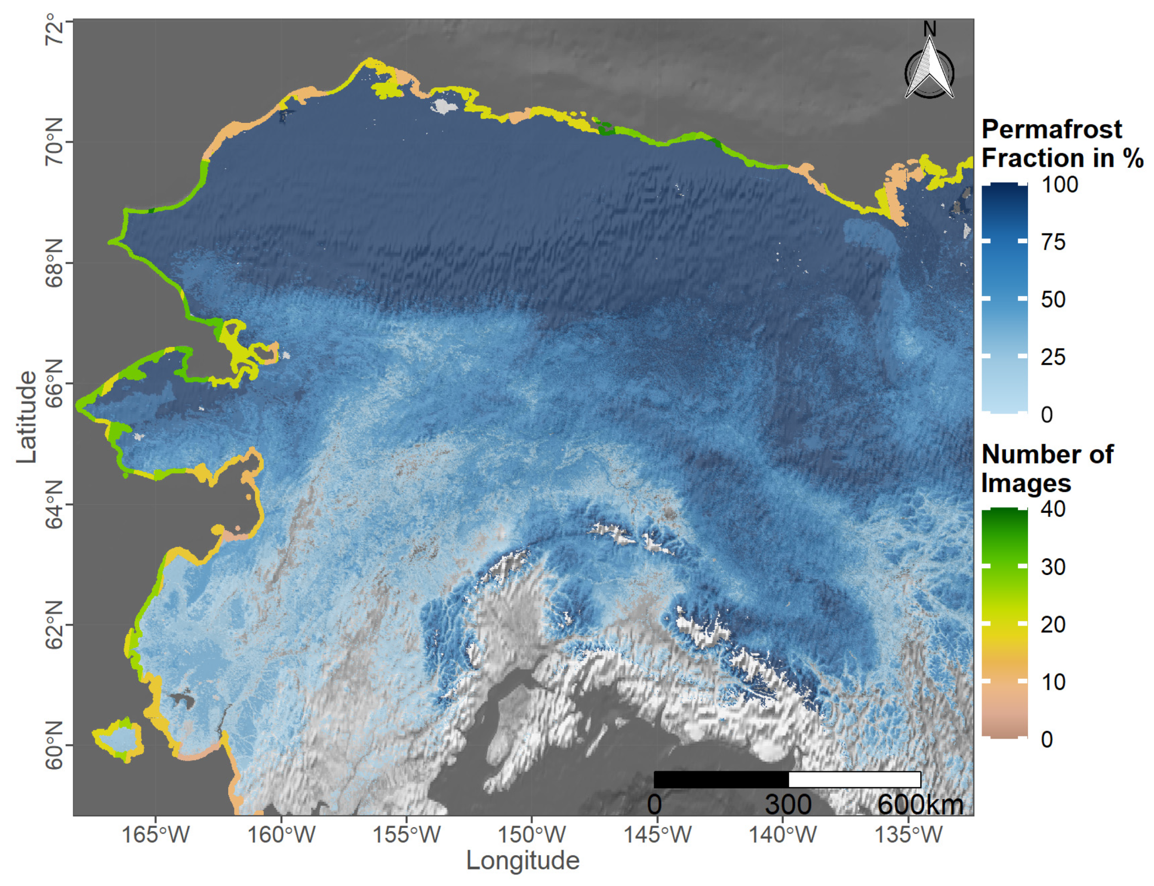
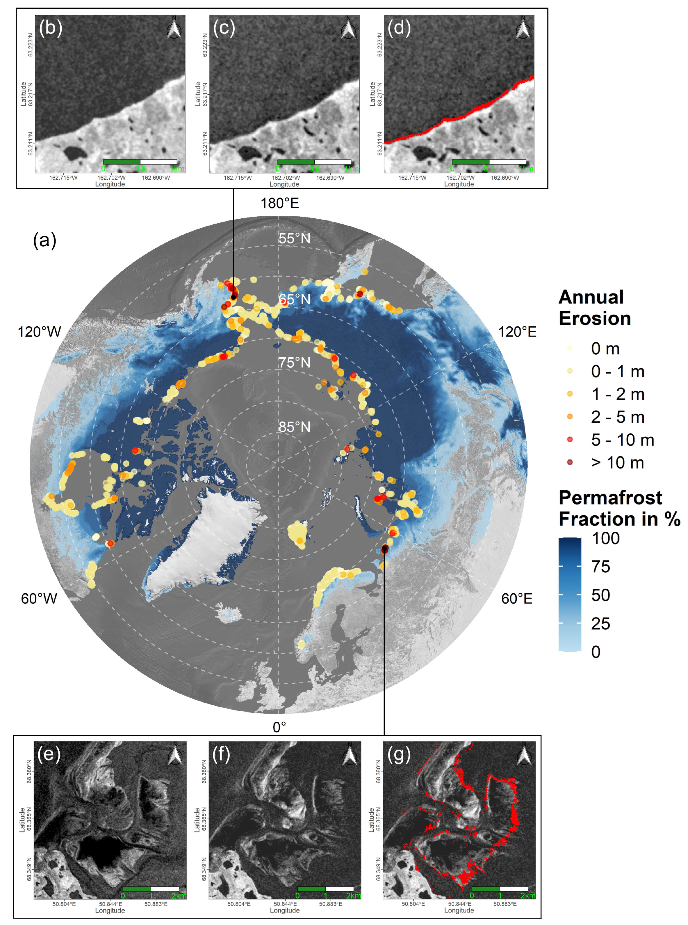
2.1. Study Area
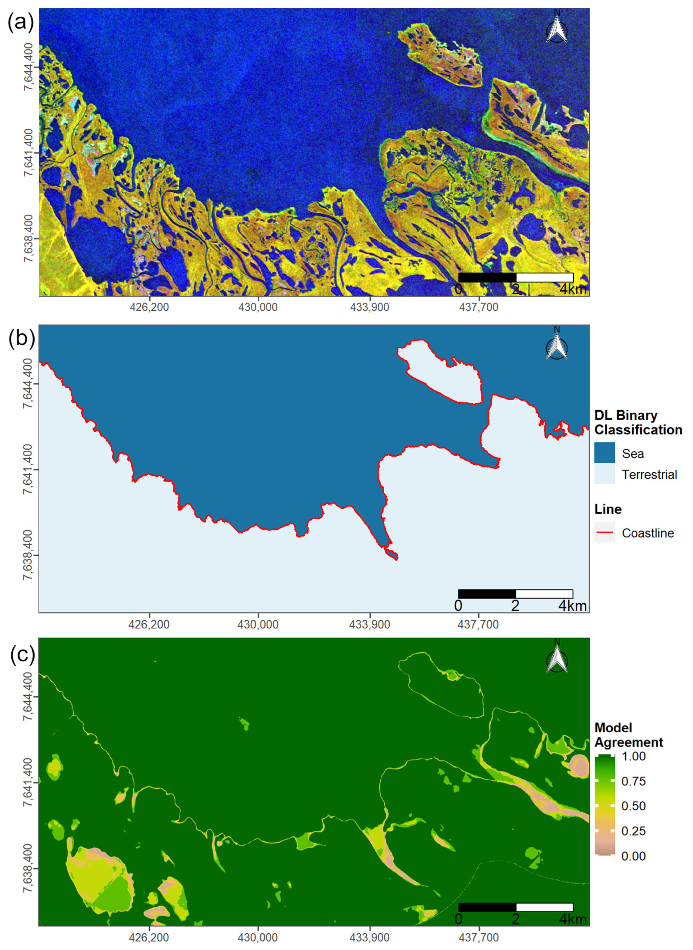
2.2. Framework for Deep Learning-Based Arctic Coastline Extraction
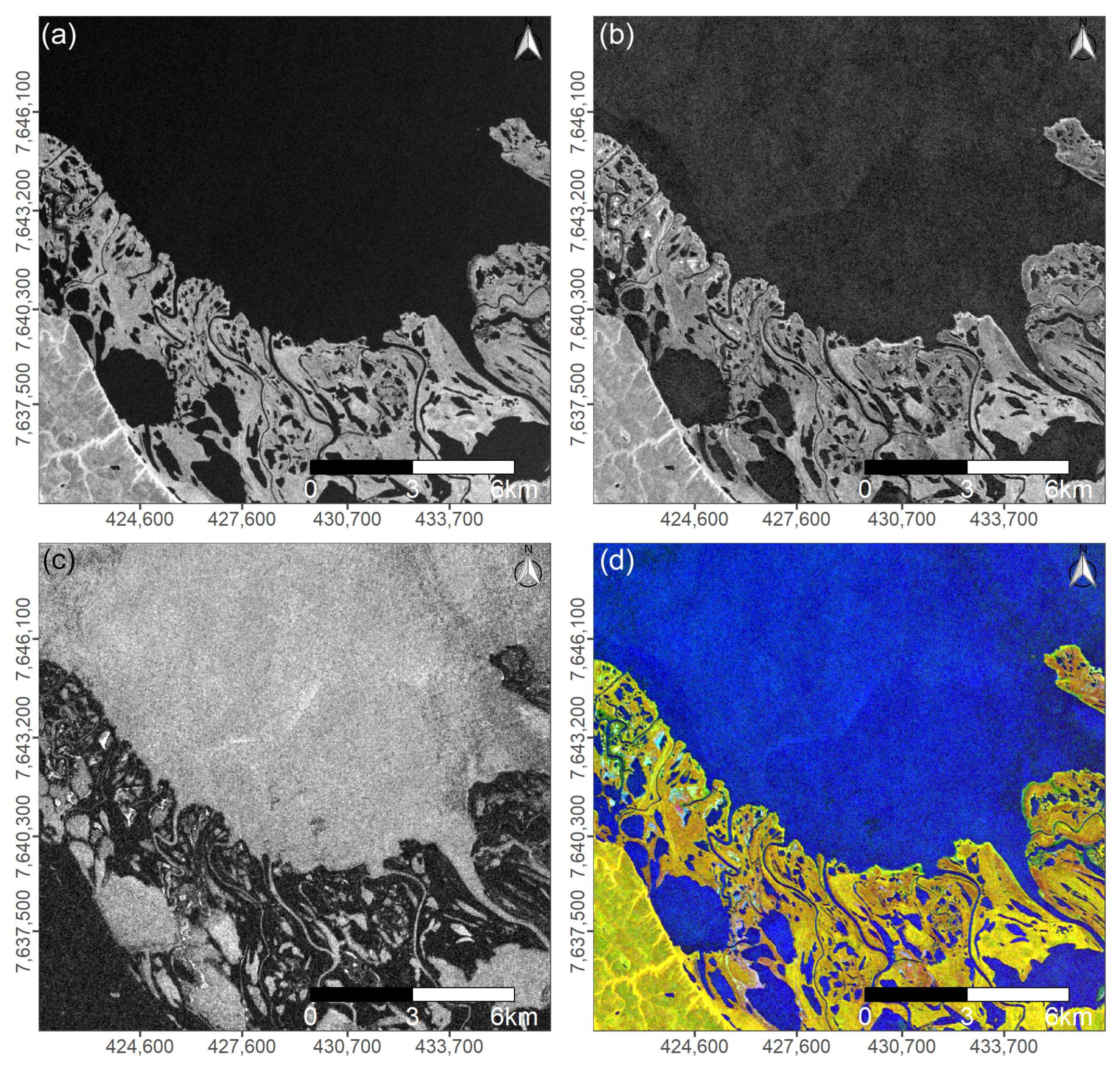
2.2.1. Preparation of Sentinel-1 Pseudo-RGB Images
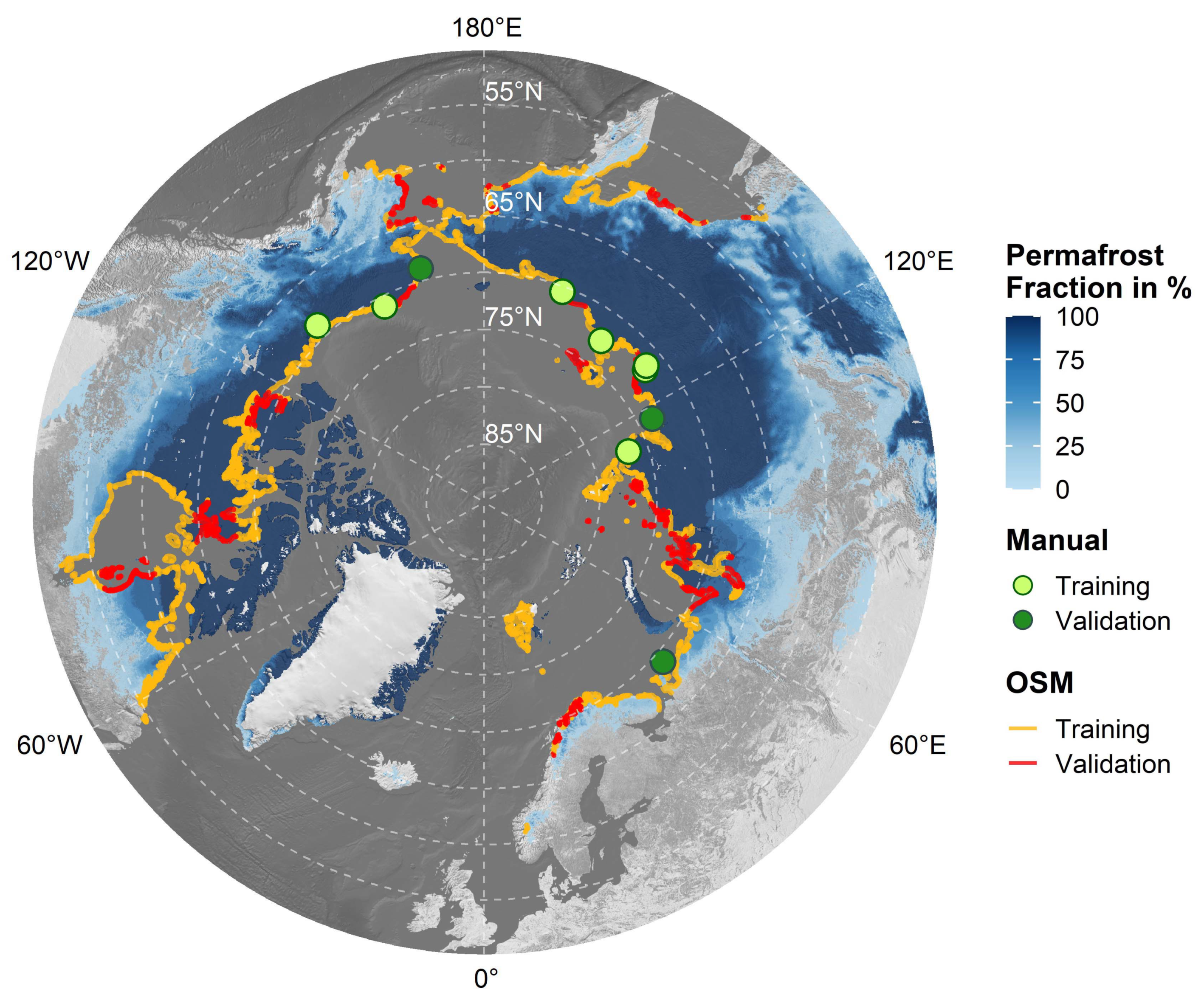
2.2.2. Preparation of Training and Validation Data
2.2.3. Deep Learning Coastline Detection
- = Number of occurrences of the mode value;
- = Total number of models;
- = Total number of classes.
2.3. Quantification of Coastal Change
2.3.1. Magnitude of Change via Change Vector Analysis
2.3.2. Post-Processing of Change Vector Analysis
- = Average change (either erosion or build-up) per segment in meters;
- = Length of the rectangular observation window in meters;
- = Number of pixels that indicate change (either erosion or build-up);
- = Total number of pixels in the observed window.
2.4. Validation and Quality Control
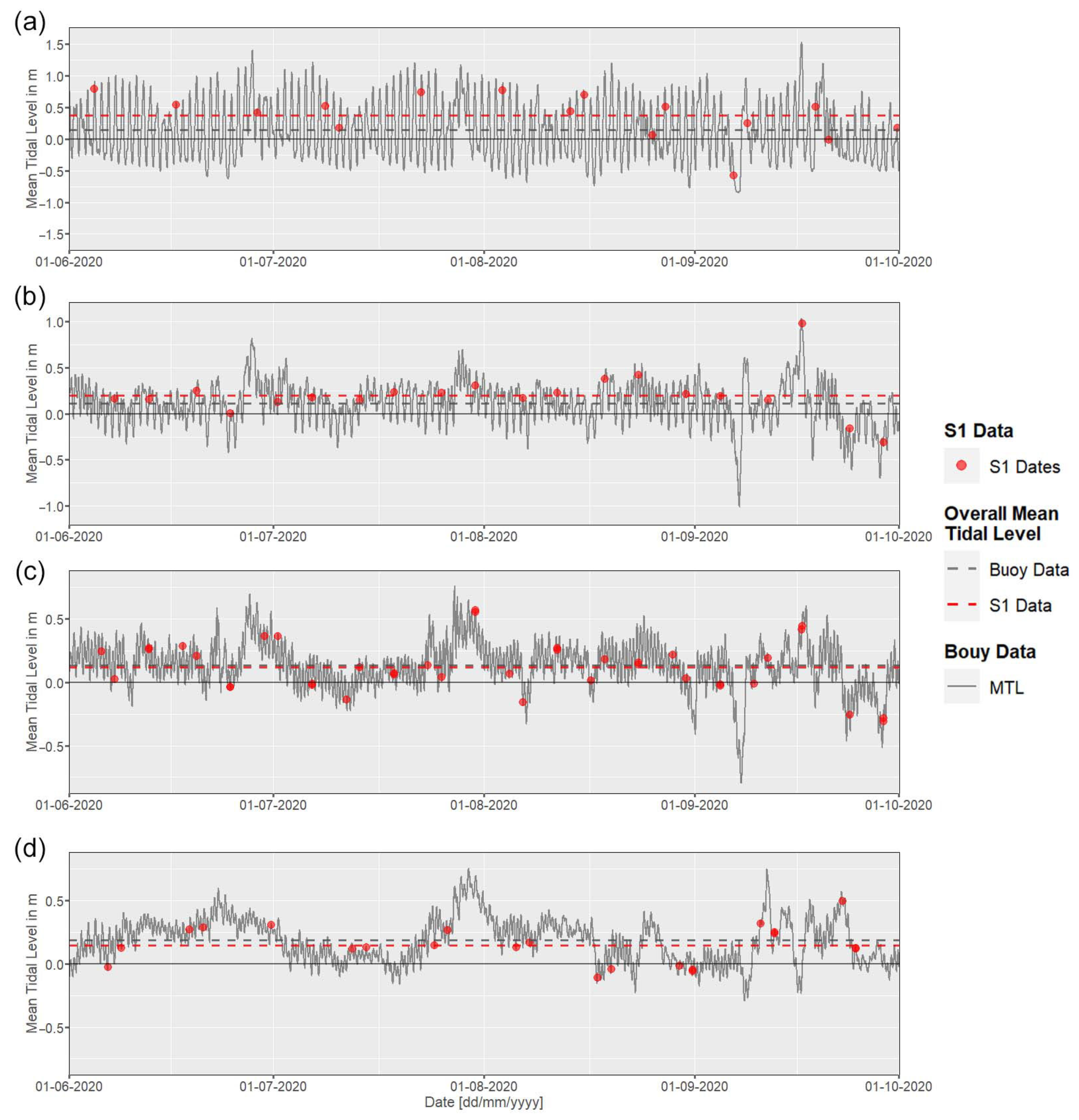
2.4.1. Tidal Influence on the Accuracy of the SAR-Based Coastline
2.4.2. Accuracy Assessment of Deep Learning Coastline
2.4.3. Accuracy Assessment Coastal Change via Change Vector Analysis
3. Results
3.1. Deep Learning Coastline Detection
3.2. Coastal Erosion and Build-Up Rates
4. Discussion
4.1. A Deep Learning-Based Circum-Arctic Coastline Product
4.2. Quantifying Coastal Change via Change Vector Analysis
4.3. Limitations and Future Potentials
5. Conclusions
- Despite fluctuations in data quality, OpenStreetMap (OSM) proved to be a feasible additional input for training Convolutional Neural Networks (CNN) U-Net architectures on the segmentation between sea and terrestrial areas in Arctic environments.
- DL in combination with annual median and sd backscatter from S1 allowed for the computation of a high-quality reference coastline with a total length of 161,600 km. A median accuracy of ±6.3 m to the manually digitized reference coastline and a median agreement of ±29.6 m to the OSM reference coastline was achieved.
- A good agreement between the average Mean Tidal Level (MTL) from S1 acquisition dates and the actual MTL was observed (±0.02–0.23 m). The higher the number of available S1 scenes, the smaller the gap between the MTL represented by the S1 acquisition dates and the actual average MTL for a given observation period.
- The inverse behavior of median and sd backscatter over sea and terrestrial areas could be successfully exploited for the CVA analysis. However, the quality and applicability of the analysis strongly depend on the number of available scenes, the present coast type, and total sea ice duration during the observed temporal window.
- Maximum annual erosion rates of up to 67 m were observed in Russia, followed by 62.5 m in Alaska. Overall average annual erosion was highest in the United States with 0.75 m, followed by Russia with 0.62 m. The weakest average annual erosion was observed in Norway (0.01 m). The Beaufort Sea featured the overall strongest annual average erosion of 1.12 m across all seas. Statistics are hereby based on all segments, including segments without coastal change.
- In total, 12.24% of the entire investigated Arctic coastline indicated an average annual erosion rate of 3.8 m and a combined 17.83 km of eroded land area per year, while 1.05% of the coastline featured an average annual build-up rate of 2.3 m and a combined annual build-up area of 1.02 km.
- Quality layers in the form of the number of available images, number of sea ice days, model agreement, and the presence/absence of glaciers are provided on a pixel basis. The aforementioned quality layers may act as helpful proxies for assessing the applicability of the proposed methods and data, and the quality of the output products.
Author Contributions
Funding
Data Availability Statement
Conflicts of Interest
Abbreviations
| ACD | Arctic Coastal Dynamics Database |
| AMIS | Agricultural Market Information System |
| ASI | ARTIST Sea Ice |
| CCI | Climate Change Initiative |
| CNES | Centre national d’études spatiales |
| CNN | Convolutional Neural Network |
| CVA | Change Vector Analysis |
| dB | decibel |
| DL | Deep Learning |
| DLR | German Aerospace Center |
| EOC | Earth Observation Center |
| FAO | Food and Agriculture Organization of the United Nations |
| GAUL | Global Administrative Unit Layers |
| GEE | Google Earth Engine |
| GLIMS | Global Land Ice Measurements from Space |
| GMT | Greenwich Mean Time |
| GPS | Global Positioning System |
| GRD | Ground Range Detected |
| IHO | International Hydrographic Organization |
| IW | Interferometric Wide |
| MTL | Mean Tidal Level |
| MV | Moving Window |
| OSM | OpenStreetMap |
| RGB | Red Green Blue |
| RMSprop | Root Mean Squared Propagation |
| S1 | Sentinel-1 |
| S2 | Sentinel-2 |
| SAR | Synthetic Aperture RADAR |
| sd | standard deviation |
| VGI | Volunteered Geographic Information |
| VH | vertical-horizontal |
| VV | vertical-vertical |
Appendix A

| Model | Epoch | Training Acc. | Training Loss | Validation Acc. | Validation Loss |
|---|---|---|---|---|---|
| DenseNet121 | 18 | 0.9894 | 0.0311 | 0.9796 | 0.1003 |
| Inception-ResNet v | 20 | 0.9933 | 0.0175 | 0.9796 | 0.1160 |
| Inception v3 | 29 | 0.9952 | 0.0121 | 0.9785 | 0.1508 |
| ResNet34 | 4 | 0.9838 | 0.0488 | 0.9790 | 0.0696 |
| ResNet50 | 27 | 0.9900 | 0.0276 | 0.9787 | 0.1000 |
| ResNeXt50 | 23 | 0.9885 | 0.0323 | 0.9805 | 0.0844 |
| SE-ResNeXt50 | 20 | 0.9941 | 0.0155 | 0.9799 | 0.1080 |
| VGG16 | 29 | 0.9945 | 0.0143 | 0.9787 | 0.1283 |
| VGG19 | 12 | 0.9900 | 0.0289 | 0.9787 | 0.0881 |
References
- Bartsch, A.; Höfler, A.; Kroisleitner, C.; Trofaier, A.M. Land cover mapping in northern high latitude permafrost regions with satellite data: Achievements and remaining challenges. Remote Sens. 2016, 8, 979. [Google Scholar] [CrossRef] [Green Version]
- Trofaier, A.M.; Westermann, S.; Bartsch, A. Progress in space-borne studies of permafrost for climate science: Towards a multi-ECV approach. Remote Sens. Environ. 2017, 203, 55–70. [Google Scholar] [CrossRef]
- Schuur, E.A.; McGuire, A.D.; Schädel, C.; Grosse, G.; Harden, J.; Hayes, D.J.; Hugelius, G.; Koven, C.D.; Kuhry, P.; Lawrence, D.M.; et al. Climate change and the permafrost carbon feedback. Nature 2015, 520, 171–179. [Google Scholar] [CrossRef] [PubMed]
- Pörtner, H.O.; Roberts, D.C.; Masson-Delmotte, V.; Zhai, P.; Tignor, M.; Poloczanska, E.; Mintenbeck, K.; Nicolai, M.; Okem, A.; Petzold, J.; et al. IPCC Special Report on the Ocean and Cryosphere in a Changing Climate; IPCC Intergovernmental Panel on Climate Change (IPCC): Geneva, Switzerland, 2019. [Google Scholar]
- Romanovsky, V.E.; Smith, S.L.; Christiansen, H.H. Permafrost thermal state in the polar Northern Hemisphere during the international polar year 2007–2009: A synthesis. Permafr. Periglac. Process. 2010, 21, 106–116. [Google Scholar] [CrossRef] [Green Version]
- Biskaborn, B.K.; Smith, S.L.; Noetzli, J.; Matthes, H.; Vieira, G.; Streletskiy, D.A.; Schoeneich, P.; Romanovsky, V.E.; Lewkowicz, A.G.; Abramov, A.; et al. Permafrost is warming at a global scale. Nat. Commun. 2019, 10, 1–11. [Google Scholar] [CrossRef] [Green Version]
- Slater, A.G.; Lawrence, D.M. Diagnosing present and future permafrost from climate models. J. Clim. 2013, 26, 5608–5623. [Google Scholar] [CrossRef] [Green Version]
- Pastick, N.J.; Jorgenson, M.T.; Wylie, B.K.; Nield, S.J.; Johnson, K.D.; Finley, A.O. Distribution of near-surface permafrost in Alaska: Estimates of present and future conditions. Remote Sens. Environ. 2015, 168, 301–315. [Google Scholar] [CrossRef] [Green Version]
- Whiteman, G.; Hope, C.; Wadhams, P. Vast costs of Arctic change. Nature 2013, 499, 401–403. [Google Scholar] [CrossRef]
- Günther, F.; Overduin, P.P.; Sandakov, A.V.; Grosse, G.; Grigoriev, M.N. Short-and long-term thermo-erosion of ice-rich permafrost coasts in the Laptev Sea region. Biogeosciences 2013, 10, 4297–4318. [Google Scholar] [CrossRef] [Green Version]
- Novikova, A.; Belova, N.; Baranskaya, A.; Aleksyutina, D.; Maslakov, A.; Zelenin, E.; Shabanova, N.; Ogorodov, S. Dynamics of permafrost coasts of Baydaratskaya Bay (Kara Sea) based on multi-temporal remote sensing data. Remote Sens. 2018, 10, 1481. [Google Scholar] [CrossRef] [Green Version]
- Obu, J.; Lantuit, H.; Grosse, G.; Günther, F.; Sachs, T.; Helm, V.; Fritz, M. Coastal erosion and mass wasting along the Canadian Beaufort Sea based on annual airborne LiDAR elevation data. Geomorphology 2017, 293, 331–346. [Google Scholar] [CrossRef] [Green Version]
- Jones, B.M.; Irrgang, A.M.; Farquharson, L.M.; Lantuit, H.; Whalen, D.; Ogorodov, S.; Grigoriev, M.; Tweedie, C.; Gibbs, A.E.; Strzelecki, M.C.; et al. Coastal Permafrost Erosion; Arctic Report Card; Pacific Coastal and Marine Science Center: Santa Cruz, CA, USA, 2020; Volume 15. [Google Scholar]
- Lantuit, H.; Overduin, P.P.; Couture, N.; Wetterich, S.; Aré, F.; Atkinson, D.; Brown, J.; Cherkashov, G.; Drozdov, D.; Forbes, D.L.; et al. The Arctic coastal dynamics database: A new classification scheme and statistics on Arctic permafrost coastlines. Estuaries Coasts 2012, 35, 383–400. [Google Scholar] [CrossRef] [Green Version]
- Irrgang, A.M.; Bendixen, M.; Farquharson, L.M.; Baranskaya, A.V.; Erikson, L.H.; Gibbs, A.E.; Ogorodov, S.A.; Overduin, P.P.; Lantuit, H.; Grigoriev, M.N.; et al. Drivers, dynamics and impacts of changing Arctic coasts. Nat. Rev. Earth Environ. 2022, 3, 39–54. [Google Scholar] [CrossRef]
- Hakkinen, S.; Proshutinsky, A.; Ashik, I. Sea ice drift in the Arctic since the 1950s. Geophys. Res. Lett. 2008, 35, GL034791. [Google Scholar] [CrossRef] [Green Version]
- Cohen, J.; Screen, J.A.; Furtado, J.C.; Barlow, M.; Whittleston, D.; Coumou, D.; Francis, J.; Dethloff, K.; Entekhabi, D.; Overland, J.; et al. Recent Arctic amplification and extreme mid-latitude weather. Nat. Geosci. 2014, 7, 627–637. [Google Scholar] [CrossRef] [Green Version]
- Serreze, M.C.; Barry, R.G. Processes and impacts of Arctic amplification: A research synthesis. Glob. Planet. Chang. 2011, 77, 85–96. [Google Scholar] [CrossRef]
- Alexander, M.A.; Scott, J.D.; Friedland, K.D.; Mills, K.E.; Nye, J.A.; Pershing, A.J.; Thomas, A.C. Projected sea surface temperatures over the 21st century: Changes in the mean, variability and extremes for large marine ecosystem regions of Northern Oceans. Elem. Sci. Anthr. 2018, 6, 9. [Google Scholar] [CrossRef] [Green Version]
- Farquharson, L.M.; Mann, D.; Swanson, D.; Jones, B.; Buzard, R.; Jordan, J. Temporal and spatial variability in coastline response to declining sea-ice in northwest Alaska. Mar. Geol. 2018, 404, 71–83. [Google Scholar] [CrossRef]
- Wang, M.; Overland, J.E. A sea ice free summer Arctic within 30 years? Geophys. Res. Lett. 2009, 36, GL037820. [Google Scholar] [CrossRef] [Green Version]
- Wang, M.; Overland, J.E. A sea ice free summer Arctic within 30 years: An update from CMIP5 models. Geophys. Res. Lett. 2012, 39, GL052868. [Google Scholar] [CrossRef] [Green Version]
- Mahoney, A.R.; Eicken, H.; Gaylord, A.G.; Gens, R. Landfast sea ice extent in the Chukchi and Beaufort Seas: The annual cycle and decadal variability. Cold Reg. Sci. Technol. 2014, 103, 41–56. [Google Scholar] [CrossRef]
- Crawford, A.; Stroeve, J.; Smith, A.; Jahn, A. Arctic open-water periods are projected to lengthen dramatically by 2100. Commun. Earth Environ. 2021, 2, 1–10. [Google Scholar] [CrossRef]
- Barnhart, K.R.; Miller, C.R.; Overeem, I.; Kay, J.E. Mapping the future expansion of Arctic open water. Nat. Clim. Chang. 2016, 6, 280–285. [Google Scholar] [CrossRef]
- Forbes, D.L. State of the Arctic Coast 2010: Scientific Review and Outlook; Land-Ocean Interactions in the Coastal Zone; Institute of Coastal Research: Geesthacht, Germany, 2011. [Google Scholar]
- Shadrick, J.R.; Rood, D.H.; Hurst, M.D.; Piggott, M.D.; Hebditch, B.G.; Seal, A.J.; Wilcken, K.M. Sea-level rise will likely accelerate rock coast cliff retreat rates. Nat. Commun. 2022, 13, 7005. [Google Scholar] [CrossRef]
- Oppenheimer, M.; Glavovic, B.; Hinkel, J.; van de Wal, R.; Magnan, A.K.; Abd-Elgawad, A.; Cai, R.; Cifuentes-Jara, M.; Deconto, R.M.; Ghosh, T.; et al. Sea level rise and implications for low lying islands, coasts and communities. In IPCC Special Report on the Ocean and Cryosphere in a Changing Climate; IPCC: Geneva, Switzerland, 2019. [Google Scholar]
- Jones, B.M.; Farquharson, L.M.; Baughman, C.A.; Buzard, R.M.; Arp, C.D.; Grosse, G.; Bull, D.L.; Günther, F.; Nitze, I.; Urban, F.; et al. A decade of remotely sensed observations highlight complex processes linked to coastal permafrost bluff erosion in the Arctic. Environ. Res. Lett. 2018, 13, 115001. [Google Scholar] [CrossRef]
- Jorgenson, M.T.; Grosse, G. Remote sensing of landscape change in permafrost regions. Permafr. Periglac. Process. 2016, 27, 324–338. [Google Scholar] [CrossRef]
- Overduin, P.P.; Strzelecki, M.C.; Grigoriev, M.N.; Couture, N.; Lantuit, H.; St-Hilaire-Gravel, D.; Günther, F.; Wetterich, S. Coastal changes in the Arctic. Geol. Soc. Lond. Spec. Publ. 2014, 388, 103–129. [Google Scholar] [CrossRef]
- Fritz, M.; Vonk, J.E.; Lantuit, H. Collapsing arctic coastlines. Nat. Clim. Chang. 2017, 7, 6–7. [Google Scholar] [CrossRef] [Green Version]
- Radosavljevic, B.; Lantuit, H.; Pollard, W.; Overduin, P.; Couture, N.; Sachs, T.; Helm, V.; Fritz, M. Erosion and flooding—Threats to coastal infrastructure in the Arctic: A case study from Herschel Island, Yukon Territory, Canada. Estuaries Coasts 2016, 39, 900–915. [Google Scholar] [CrossRef] [Green Version]
- Nielsen, D.M.; Pieper, P.; Barkhordarian, A.; Overduin, P.; Ilyina, T.; Brovkin, V.; Baehr, J.; Dobrynin, M. Increase in Arctic coastal erosion and its sensitivity to warming in the twenty-first century. Nat. Clim. Chang. 2022, 12, 263–270. [Google Scholar] [CrossRef]
- Couture, N.J.; Irrgang, A.; Pollard, W.; Lantuit, H.; Fritz, M. Coastal erosion of permafrost soils along the Yukon Coastal Plain and fluxes of organic carbon to the Canadian Beaufort Sea. J. Geophys. Res. Biogeosci. 2018, 123, 406–422. [Google Scholar] [CrossRef] [Green Version]
- Tanski, G.; Wagner, D.; Knoblauch, C.; Fritz, M.; Sachs, T.; Lantuit, H. Rapid CO2 release from eroding permafrost in seawater. Geophys. Res. Lett. 2019, 46, 11244–11252. [Google Scholar] [CrossRef] [Green Version]
- Vonk, J.E.; Sánchez-García, L.; Van Dongen, B.; Alling, V.; Kosmach, D.; Charkin, A.; Semiletov, I.P.; Dudarev, O.V.; Shakhova, N.; Roos, P.; et al. Activation of old carbon by erosion of coastal and subsea permafrost in Arctic Siberia. Nature 2012, 489, 137–140. [Google Scholar] [CrossRef]
- Terhaar, J.; Lauerwald, R.; Regnier, P.; Gruber, N.; Bopp, L. Around one third of current Arctic Ocean primary production sustained by rivers and coastal erosion. Nat. Commun. 2021, 12, 169. [Google Scholar] [CrossRef]
- Abbott, B.W.; Jones, J.B.; Schuur, E.A.; Chapin, F.S., III; Bowden, W.B.; Bret-Harte, M.S.; Epstein, H.E.; Flannigan, M.D.; Harms, T.K.; Hollingsworth, T.N.; et al. Biomass offsets little or none of permafrost carbon release from soils, streams, and wildfire: An expert assessment. Environ. Res. Lett. 2016, 11, 034014. [Google Scholar] [CrossRef]
- Philipp, M.; Dietz, A.; Ullmann, T.; Kuenzer, C. Automated Extraction of Annual Erosion Rates for Arctic Permafrost Coasts Using Sentinel-1, Deep Learning, and Change Vector Analysis. Remote Sens. 2022, 14, 3656. [Google Scholar] [CrossRef]
- Duncan, B.N.; Ott, L.E.; Abshire, J.B.; Brucker, L.; Carroll, M.L.; Carton, J.; Comiso, J.C.; Dinnat, E.P.; Forbes, B.C.; Gonsamo, A.; et al. Space-Based Observations for Understanding Changes in the Arctic-Boreal Zone. Rev. Geophys. 2020, 58, e2019RG000652. [Google Scholar] [CrossRef] [Green Version]
- Westermann, S.; Duguay, C.R.; Grosse, G.; Kääb, A. Chapter 13: Remote sensing of permafrost and frozen ground. In Remote Sensing of the Cryosphere; John Wiley & Sons, Ltd.: Chichester, UK, 2014; pp. 307–344. [Google Scholar] [CrossRef]
- Kääb, A. Remote sensing of permafrost-related problems and hazards. Permafr. Periglac. Process. 2008, 19, 107–136. [Google Scholar] [CrossRef]
- Bartsch, A.; Ley, S.; Nitze, I.; Pointner, G.; Vieira, G. Feasibility study for the application of Synthetic Aperture Radar for coastal erosion rate quantification across the Arctic. Front. Environ. Sci. 2020, 8, 143. [Google Scholar] [CrossRef]
- Rolph, R.; Overduin, P.P.; Ravens, T.; Lantuit, H.; Langer, M. ArcticBeach v1. 0: A physics-based parameterization of pan-Arctic coastline erosion. Front. Earth Sci. 2022, 10, 962208. [Google Scholar] [CrossRef]
- Barron, C.; Neis, P.; Zipf, A. A comprehensive framework for intrinsic OpenStreetMap quality analysis. Trans. GIS 2014, 18, 877–895. [Google Scholar] [CrossRef]
- Bansal, A.; Kauffman, R.J.; Weitz, R.R. Comparing the modeling performance of regression and neural networks as data quality varies: A business value approach. J. Manag. Inf. Syst. 1993, 10, 11–32. [Google Scholar] [CrossRef]
- Rozhnova, M. Impact of Dataset Errors on Model Accuracy. 2021. Available online: https://medium.com/deelvin-machine-learning/impact-of-dataset-errors-on-model-accuracy-723fef5e0b28 (accessed on 28 November 2022).
- ESA Communications. Sentinel-1: ESA’s Radar Observatory Mission for GMES Operational Services. 2012. Available online: https://sentinel.esa.int/documents/247904/349449/S1_SP-1322_1.pdf (accessed on 14 October 2022).
- European Space Agency. Sentinel-2 User Handbook. 2015. Available online: https://sentinels.copernicus.eu/documents/247904/685211/Sentinel-2_User_Handbook (accessed on 14 October 2022).
- Yu, L.; Gong, P. Google Earth as a virtual globe tool for Earth science applications at the global scale: Progress and perspectives. Int. J. Remote Sens. 2012, 33, 3966–3986. [Google Scholar] [CrossRef]
- Obu, J.; Westermann, S.; Barboux, C.; Bartsch, A.; Delaloye, R.; Grosse, G.; Heim, B.; Hugelius, G.; Irrgang, A.; Kääb, A.; et al. ESA Permafrost Climate Change Initiative (Permafrost_cci): Permafrost Extent for the Northern Hemisphere, v3.0’; NERC EDS Centre for Environmental Data Analysis: Norwich, UK, 2021. [CrossRef]
- OpenStreetMap Contributors. Planet Dump. 2017. Available online: https://www.openstreetmap.org (accessed on 12 November 2022).
- National Oceanic and Atmospheric Administration (NOAA). Water Levels—NOAA Tides, and Currents. 2022. Available online: https://tidesandcurrents.noaa.gov/stations.html?type=Water+Levels (accessed on 14 October 2022).
- Raup, B.; Racoviteanu, A.; Khalsa, S.J.S.; Helm, C.; Armstrong, R.; Arnaud, Y. The GLIMS geospatial glacier database: A new tool for studying glacier change. Glob. Planet. Chang. 2007, 56, 101–110. [Google Scholar] [CrossRef]
- Spreen, G.; Kaleschke, L.; Heygster, G. Sea ice remote sensing using AMSR-E 89-GHz channels. J. Geophys. Res. Ocean. 2008, 113, JC003384. [Google Scholar] [CrossRef] [Green Version]
- Flanders Marine Institute. IHO Sea Areas, Version 3. 2018. Available online: https://www.marineregions.org/ (accessed on 15 November 2022).
- Natural Earth. Natural Earth I with Shaded Relief and Water. Available online: https://www.naturalearthdata.com/downloads/10m-raster-data/10m-natural-earth-1/ (accessed on 28 August 2020).
- Cheng, D.; Meng, G.; Cheng, G.; Pan, C. SeNet: Structured edge network for sea–land segmentation. IEEE Geosci. Remote Sens. Lett. 2016, 14, 247–251. [Google Scholar] [CrossRef]
- Li, R.; Liu, W.; Yang, L.; Sun, S.; Hu, W.; Zhang, F.; Li, W. DeepUNet: A deep fully convolutional network for pixel-level sea-land segmentation. IEEE J. Sel. Top. Appl. Earth Obs. Remote Sens. 2018, 11, 3954–3962. [Google Scholar] [CrossRef] [Green Version]
- Baumhoer, C.A.; Dietz, A.J.; Kneisel, C.; Kuenzer, C. Automated extraction of antarctic glacier and ice shelf fronts from sentinel-1 imagery using deep learning. Remote Sens. 2019, 11, 2529. [Google Scholar] [CrossRef] [Green Version]
- Heidler, K.; Mou, L.; Baumhoer, C.; Dietz, A.; Zhu, X.X. HED-UNet: Combined Segmentation and Edge Detection for Monitoring the Antarctic Coastline. IEEE Trans. Geosci. Remote. Sens. 2021, 60, 4300514. [Google Scholar] [CrossRef]
- Ronneberger, O.; Fischer, P.; Brox, T. U-net: Convolutional networks for biomedical image segmentation. In Proceedings of the International Conference on Medical Image Computing and Computer-Assisted Intervention, Munich, Germany, 5–9 October 2015; pp. 234–241. [Google Scholar]
- Kääb, A.; Huggel, C.; Fischer, L.; Guex, S.; Paul, F.; Roer, I.; Salzmann, N.; Schlaefli, S.; Schmutz, K.; Schneider, D.; et al. Remote sensing of glacier- and permafrost-related hazards in high mountains: An overview. Nat. Hazards Earth Syst. Sci. 2005, 5, 527–554. [Google Scholar] [CrossRef]
- Google Developers. Sentinel-1 Algorithms. 2021. Available online: https://developers.google.com/earth-engine/guides/sentinel1 (accessed on 25 November 2022).
- OpenStreetMap. Contributors. Available online: https://wiki.openstreetmap.org/wiki/Contributors#Denmark (accessed on 22 January 2023).
- Mooney, P.; Corcoran, P.; Winstanley, A.C. Towards quality metrics for OpenStreetMap. In Proceedings of the 18th SIGSPATIAL International Conference on Advances in Geographic Information Systems, San Jose, CA, USA, 2–5 November 2010; pp. 514–517. [Google Scholar]
- He, K.; Zhang, X.; Ren, S.; Sun, J. Deep residual learning for image recognition. In Proceedings of the IEEE Conference on Computer Vision and Pattern Recognition, Las Vegas, NV, USA, 27–30 June 2016; pp. 770–778. [Google Scholar]
- Simonyan, K.; Zisserman, A. Very deep convolutional networks for large-scale image recognition. arXiv 2014, arXiv:1409.1556. [Google Scholar]
- Szegedy, C.; Vanhoucke, V.; Ioffe, S.; Shlens, J.; Wojna, Z. Rethinking the Inception Architecture for Computer Vision. In Proceedings of the IEEE Conference on Computer Vision and Pattern Recognition, Las Vegas, NV, USA, 27–30 June 2016; pp. 2818–2826. [Google Scholar]
- Szegedy, C.; Ioffe, S.; Vanhoucke, V.; Alemi, A.A. Inception-v4, inception-resnet and the impact of residual connections on learning. In Proceedings of the Thirty-first AAAI Conference on Artificial Intelligence, San Francisco, CA, USA, 4–9 February 2017. [Google Scholar]
- Huang, G.; Liu, Z.; Van Der Maaten, L.; Weinberger, K.Q. Densely connected convolutional networks. In Proceedings of the IEEE Conference on Computer Vision and Pattern Recognition, Honolulu, HI, USA, 21–26 July 2017; pp. 4700–4708. [Google Scholar]
- Xie, S.; Girshick, R.; Dollár, P.; Tu, Z.; He, K. Aggregated residual transformations for deep neural networks. In Proceedings of the IEEE Conference on Computer Vision and Pattern Recognition, Honolulu, HI, USA, 21–26 July 2017; pp. 1492–1500. [Google Scholar]
- Hu, J.; Shen, L.; Sun, G. Squeeze-and-excitation networks. In Proceedings of the IEEE Conference on Computer Vision and Pattern Recognition, Salt Lake City, UT, USA, 18–22 June 2018; pp. 7132–7141. [Google Scholar]
- Wegmann, M.; Leutner, B.; Dech, S. Remote Sensing and GIS for Ecologists: Using Open Source Software; Pelagic Publishing Ltd.: Exeter, UK, 2016. [Google Scholar]
- Chen, J.; Chen, X.; Cui, X.; Chen, J. Change vector analysis in posterior probability space: A new method for land cover change detection. IEEE Geosci. Remote Sens. Lett. 2010, 8, 317–321. [Google Scholar] [CrossRef]
- GLIMS Consortium. GLIMS Glacier Database, Version 1. 2005. Available online: https://nsidc.org/data/NSIDC-0272/versions/1 (accessed on 7 November 2022).
- National Oceanic and Atmospheric Administration (NOAA). Tidal Datums—NOAA Tides, and Currents. 2022. Available online: https://tidesandcurrents.noaa.gov/datum_options.html (accessed on 14 October 2022).
- Schubert, A.; Small, D.; Miranda, N.; Geudtner, D.; Meier, E. Sentinel-1A product geolocation accuracy: Commissioning phase results. Remote Sens. 2015, 7, 9431–9449. [Google Scholar] [CrossRef] [Green Version]
- Schubert, A.; Miranda, N.; Geudtner, D.; Small, D. Sentinel-1A/B combined product geolocation accuracy. Remote Sens. 2017, 9, 607. [Google Scholar] [CrossRef] [Green Version]
- Richards, J.A. Remote Sensing with Imaging Radar; Springer: Berlin/Heidelberg, Germany, 2009; Volume 1, pp. 172–173. [Google Scholar]
- Lighthill, M.J.; Lighthill, J. Waves in Fluids; Cambridge University Press: Cambridge, MA, USA, 2001; p. 205. [Google Scholar]
- Tang, C.; Zhu, Q.; Wu, W.; Huang, W.; Hong, C.; Niu, X. PLANET: Improved convolutional neural networks with image enhancement for image classification. Math. Probl. Eng. 2020, 2020, 1245924. [Google Scholar] [CrossRef]
- Klein, B.; Rossin, D. Data quality in neural network models: Effect of error rate and magnitude of error on predictive accuracy. Omega 1999, 27, 569–582. [Google Scholar] [CrossRef]
- Zhou, Z.; Siddiquee, M.M.R.; Tajbakhsh, N.; Liang, J. Unet++: Redesigning skip connections to exploit multiscale features in image segmentation. IEEE Trans. Med Imaging 2019, 39, 1856–1867. [Google Scholar] [CrossRef] [Green Version]
- Wang, J.; Li, D.; Cao, W.; Lou, X.; Shi, A.; Zhang, H. Remote Sensing Analysis of Erosion in Arctic Coastal Areas of Alaska and Eastern Siberia. Remote Sens. 2022, 14, 589. [Google Scholar] [CrossRef]
- Irrgang, A.M.; Lantuit, H.; Manson, G.K.; Günther, F.; Grosse, G.; Overduin, P.P. Variability in rates of coastal change along the Yukon coast, 1951 to 2015. J. Geophys. Res. Earth Surf. 2018, 123, 779–800. [Google Scholar] [CrossRef] [Green Version]
- European Space Agency. Observation Scenario Archive. Available online: https://sentinels.copernicus.eu/web/sentinel/missions/sentinel-1/observation-scenario/archive (accessed on 2 December 2022).
- Alaska Satellite Facility. Sentinel-1—Acquisition Maps. Available online: https://asf.alaska.edu/data-sets/sar-data-sets/sentinel-1/sentinel-1-acquisition-maps/ (accessed on 28 November 2022).
- European Space Agency. Mission Ends for Copernicus Sentinel-1B Satellite. Available online: https://www.esa.int/Applications/Observing_the_Earth/Copernicus/Sentinel-1/Mission_ends_for_Copernicus_Sentinel-1B_satellite (accessed on 29 November 2022).
- Ekman, M. A consistent map of the postglacial uplift of Fennoscandia. Terra Nova 1996, 8, 158–165. [Google Scholar] [CrossRef]


| Name | Data Type | Spatial Resolution | Temporal Coverage & Resolution | Reference |
|---|---|---|---|---|
| Sentinel-1 Ground Range Detected (GRD) Interferometric Wide (IW) swath | Raster | 10 m | 2017–2021 (up to 6 days) | [49] |
| Sentinel-2 | Raster | 10 m | 2017–2021 (up to 5 days) | [50] |
| Google Earth | Raster | varies | 2017–2021 (varies) | [51] |
| Climate Change Initiative (CCI) Permafrost Fraction | Raster | 927 m | 2017 | [52] |
| OpenStreetMap (OSM) | Vector | - | 2022 | [53] |
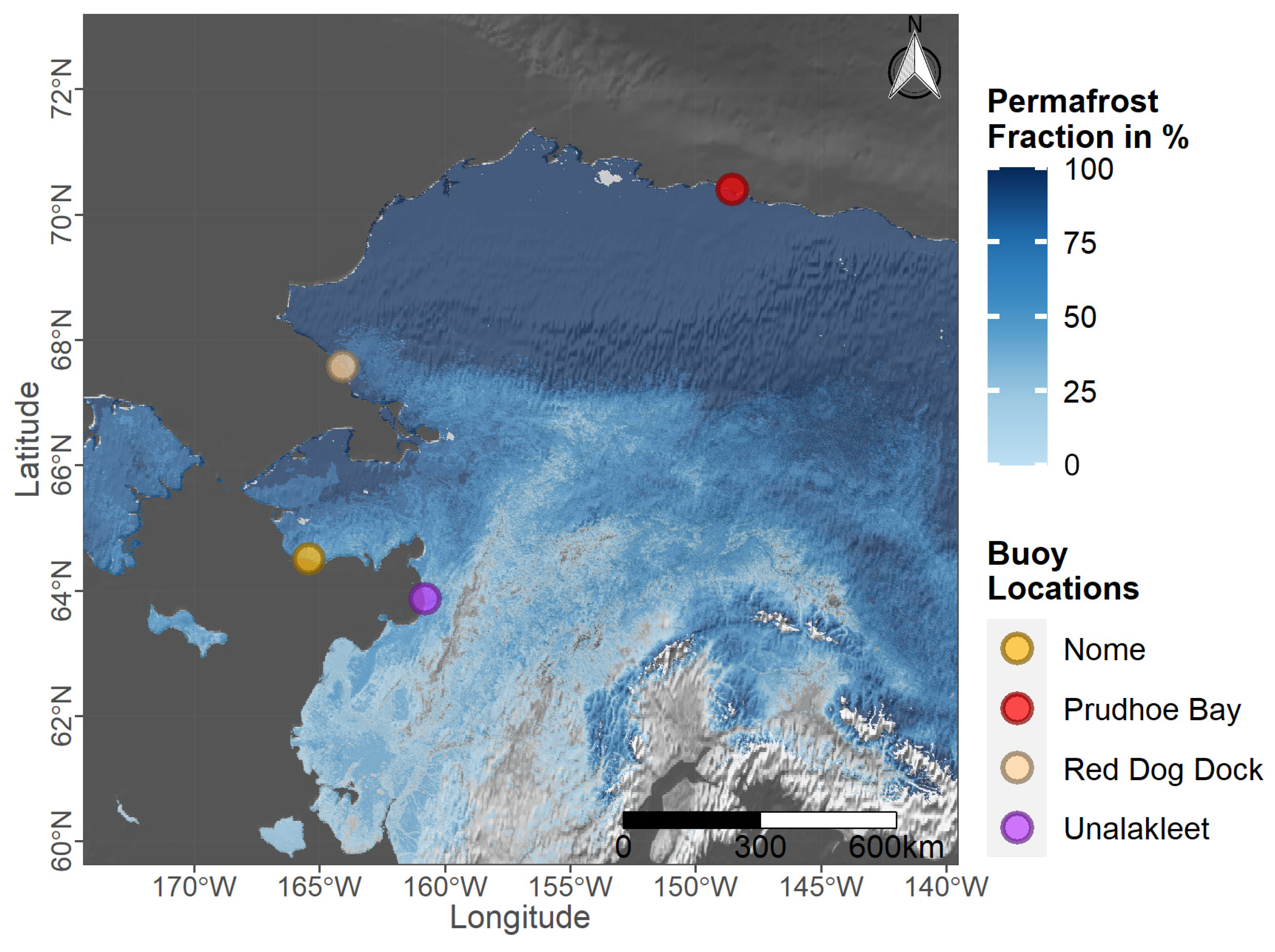
| Buoy Mean Tidal Level (MTL) Data | Table | - | 2020 (6 min) | [54] |
| Global Land Ice Measurements from Space (GLIMS) glacier database | Vector | - | 2022 | [55] |
| ARTIST Sea Ice (ASI) Arctic Sea Ice Concentration | Raster | 3125 m | 2017–2021 (daily) | [56] |
| Arctic Coastal Dynamics Database (ACD) Database | Vector | - | 2012 | [14] |
| International Hydrographic Organization (IHO) Sea Areas | Vector | - | 2018 | [57] |
| Manually Digitized Sites | |||||
|---|---|---|---|---|---|
| Area | Overall Acc. | Label | Precision | Recall | F1 |
| Training | 0.95 | Terrestrial | 0.97 | 0.93 | 0.95 |
| Sea | 0.93 | 0.97 | 0.95 | ||
| Validation | 0.97 | Terrestrial | 0.98 | 0.96 | 0.97 |
| Sea | 0.96 | 0.98 | 0.97 | ||
| OpenStreetMap (OSM) Sites | |||||
| Area | Overall Acc. | Label | Precision | Recall | F1 |
| Training | 0.95 | Terrestrial | 0.92 | 0.97 | 0.94 |
| Sea | 0.97 | 0.93 | 0.95 | ||
| Validation | 0.94 | Terrestrial | 0.90 | 0.99 | 0.94 |
| Sea | 0.99 | 0.91 | 0.95 | ||
| Sea | Mean | Max | SD | Perc. |
|---|---|---|---|---|
| Bering Sea | 0.65 m (0.02 m) | 62.5 m (19 m) | 3.26 m (0.28 m) | 14.39% (1.13%) |
| Chukchi Sea | 0.19 m (0.01 m) | 26 m (11.25 m) | 1.06 m (0.21 m) | 10.02% (0.69%) |
| Beaufort Sea | 1.12 m (0.02 m) | 46 m (14.75 m) | 3.38 m (0.35 m) | 47.24% (1.32%) |
| Labrador Sea | 0.05 m (0 m) | 13 m (2.25 m) | 0.38 m (0.02 m) | 3.89% (0.07%) |
| Hudson Strait | 0.5 m (0.05 m) | 39 m (17.50 m) | 2.33 m (0.64 m) | 20.85% (2.07%) |
| Davis Strait | 0.73 m (0 m) | 38.75 m (0 m) | 3.03 m (0 m) | 18.92% (0%) |
| East Siberian Sea | 0.91 m (0.03 m) | 33.25 m (10 m) | 2.66 m (0.34 m) | 39.31% (2.66%) |
| Hudson Bay | 0.22 m (0.02 m) | 40 m (18.25 m) | 1.43 m (0.37 m) | 12.62% (1.22%) |
| The Northwestern Passages | 0.22 m (0 m) | 28.25 m (3.50 m) | 1.31 m (0.09 m) | 8.81% (0.30%) |
| Arctic Ocean | 0.05 m (0.01 m) | 3.67 m (1 m) | 0.31 m (0.1 m) | 3.72% (2.80%) |
| Barents Sea | 0.69 m (0.03 m) | 67 m (52.67 m) | 3.63 m (0.97 m) | 9.81% (0.91%) |
| Greenland Sea | 0.09 m (0.02 m) | 39.33 m (12.67 m) | 1.08 m (0.37 m) | 4.08% (1%) |
| Sea of Okhotsk | 0.56 m (0.09 m) | 43.75 m (23.75 m) | 2.89 m (0.93 m) | 12% (1.66%) |
| Kara Sea | 0.59 m (0.02 m) | 51.75 m (5.5 m) | 2.77 m (0.22 m) | 21.28% (1.92%) |
| Laptev Sea | 0.25 m (0.07 m) | 42 m (53.25 m) | 1.83 m (1.17 m) | 10.51% (1.67%) |
| Norwegian Sea | 0.01 m (0 m) | 18 m (5 m) | 0.26 m (0.08 m) | 0.75% (0.38%) |
| Country | Mean | Max | SD | Perc. |
|---|---|---|---|---|
| United States (Alaska) | 0.75 m (0.01 m) | 62.5 m (14.75 m) | 3.45 m (0.25 m) | 17.82% (1.05%) |
| Canada | 0.24 m (0.01 m) | 40 m (18.25 m) | 1.42 m (0.27 m) | 11.82% (0.67%) |
| Norway (Svalbard and Jan Mayen) | 0.09 m (0.07 m) | 39.33 m (52.67 m) | 1.01 m (1.62 m) | 4.06% (1.11%) |
| Norway (Scandinavian Peninsula) | 0.01 m (0 m) | 18 m (5 m) | 0.21 m (0.08 m) | 0.53% (0.32%) |
| Russia | 0.62 m (0.04 m) | 67 m (53.25 m) | 3.01 m (0.65 m) | 16.61% (1.68%) |
Disclaimer/Publisher’s Note: The statements, opinions and data contained in all publications are solely those of the individual author(s) and contributor(s) and not of MDPI and/or the editor(s). MDPI and/or the editor(s) disclaim responsibility for any injury to people or property resulting from any ideas, methods, instructions or products referred to in the content. |
© 2023 by the authors. Licensee MDPI, Basel, Switzerland. This article is an open access article distributed under the terms and conditions of the Creative Commons Attribution (CC BY) license (https://creativecommons.org/licenses/by/4.0/).
Share and Cite
Philipp, M.; Dietz, A.; Ullmann, T.; Kuenzer, C. A Circum-Arctic Monitoring Framework for Quantifying Annual Erosion Rates of Permafrost Coasts. Remote Sens. 2023, 15, 818. https://doi.org/10.3390/rs15030818
Philipp M, Dietz A, Ullmann T, Kuenzer C. A Circum-Arctic Monitoring Framework for Quantifying Annual Erosion Rates of Permafrost Coasts. Remote Sensing. 2023; 15(3):818. https://doi.org/10.3390/rs15030818
Chicago/Turabian StylePhilipp, Marius, Andreas Dietz, Tobias Ullmann, and Claudia Kuenzer. 2023. "A Circum-Arctic Monitoring Framework for Quantifying Annual Erosion Rates of Permafrost Coasts" Remote Sensing 15, no. 3: 818. https://doi.org/10.3390/rs15030818
APA StylePhilipp, M., Dietz, A., Ullmann, T., & Kuenzer, C. (2023). A Circum-Arctic Monitoring Framework for Quantifying Annual Erosion Rates of Permafrost Coasts. Remote Sensing, 15(3), 818. https://doi.org/10.3390/rs15030818