Analysis of Post-Mining Vegetation Development Using Remote Sensing and Spatial Regression Approach: A Case Study of Former Babina Mine (Western Poland)

Abstract

The vegetation of the post-mining areas is subject to constant and significant changes. Reclamation works, carried out after the cessation of mineral extraction, contribute to the intensive development of new plant species. However, secondary deformations, occurring even many years after the end of exploitation, may cause the degradation of the vegetation cover. It is, therefore, an important issue to identify changes in flora conditions and to determine whether and to what extent past mining has a negative impact on the plant cover state. The objectives of this research have been as follows: (1) analysis of the flora condition in the post-mining area in the 1989–2019 period, (2) identification of sites with significant changes in vegetation state, and (3) modeling of the relationship between the identified changes in vegetation and former mining activities. The research was carried out in the area of the former opencast and underground lignite mine “Friendship of Nations—Babina Shaft,” which is located in the present-day Geopark (Western Poland), using Landsat TM/ETM+/OLI derived vegetation indices (NDVI, NDII, MTVI2) and GIS-based spatial regression. The results indicate a general improvement in flora condition, especially in the vicinity of post-mining waste heaps and former opencast excavations, with the exception of the northwestern part of the former mining field where the values of all of the analyzed vegetation indices have decreased. Also, four zones of statistically significant changes in the flora condition were identified. Finally, the developed GWR models demonstrate that former mining activities had a significant influence on changes in the plant cover state of the analyzed region.

1. Introduction

Mining of raw materials inherently contributes to the degradation of land. The impacts of extracting minerals from deposits with surface or underground mining methods include continuous (e.g., subsidence basins) and discontinuous (e.g., sinkholes, cracks, throughs) deformations, large-scale earthworks (open-pits, waste dumps), lowering of the groundwater table (mine drainage), soil and groundwater contamination (leakages of substances during technological processes), and dust pollution. All of these effects contribute to the destruction or damage of vegetation in and around the mining area [1,2,3,4].

The increasing number of post-mining sites worldwide requires effective and reliable methods of monitoring the condition of these areas. Kretschmann and Nguyen [5] state that the processes affecting the post-mining environment should be regarded as continuous and treated as such. For example, secondary ground deformations may occur decades after the end of the underground extraction of minerals [6] in the form of residual subsidence [7,8]. Uplift is caused by a change of rock mass conditions due to the saturation of the previously drained rock formations [9,10,11,12], while discontinuous deformations occur due to the destruction of old, especially shallow, voids underground [13,14]. The subsided zones may experience waterlogging or flooding resulting from the restoration of the original groundwater table. All the above-mentioned phenomena have a significant impact on the vegetation of the post-mining areas.

The areas degraded by mining (usually surface mining) are subjected to technical and biological treatments aimed at restoring their value. The subsequent stages of the reclamation process include land forming, regulating water conditions, and restoring or improving the physical and chemical properties of soils [15]. The last stage of reclamation consists of the introduction of vegetation and systematic care [16]. As a result, areas severely affected by mining may again be characterized by healthy and species-rich vegetation.

The complexity of the reclamation process and the secondary consequences of mining require continuous monitoring. It is usually limited in space and time, costly, and difficult to implement given the size of post-mining areas. However, the proliferation of open and publicly available satellite remotely sensed data and GIS-based spatiotemporal analysis methods facilitate environmental studies of former mining areas. Nowadays, the analysis of vegetation cover conditions in post-mining areas is based on spectral indices, determined from remotely sensed imagery and processed in Geographic Information Systems (GIS). The former enables the study of biophysical and biochemical parameters of the flora; the latter is used for spatiotemporal analyses and data visualization. Among the published studies of vegetation cover conditions in post-mining areas that are based on vegetation indices, those related to the monitoring and evaluation of the reclamation process have been the most frequent. Noteworthy examples include Karan et al. [17] who have used NDVI, RVI, EVI, and NDMI indices, derived from Landsat TM/OLI images and the Support Vector Machine (SVM) algorithm to identify spatiotemporal changes in the flora of the Jharia hard coal mining area in the 2000–2015 period. Padró et al. [18] have used high-resolution multispectral imagery acquired with an Unmanned Aerial System (UAV) and SAVI, MSAVI, NDVI, and NDWI indices to evaluate vegetation development in a restored calcareous quarry. Yao and Zhou Wei [19] have applied as many as 19 vegetation indices to assess the process of restoration in the Pingshuo Coal Mining area. The authors relied on the Landsat TM imagery registered between 1990 and 2019 and the Principal Component Analysis (PCA) method. The results of other significant studies aimed at assessment of the post-mining area’s restoration using spectral indices have also been presented in [20,21,22,23,24,25,26,27,28,29]. Vegetation indices based on remotely sensed data have been used in studies concerning: the assessment of surface mining and reclamation process impacts on croplands and food security [30], analysis of the relation between metal concentration and reflectance spectra of plant leaves [31], evaluation of the change in surface mining and restored areas in time [32,33], detection of spontaneous combustion of coal waste dumps [34], assessment of biomass production [35], and effect of aggregated mining development on the condition of vegetation [29]. More examples of such studies can be found in review publications [36,37].

The GIS methods were used in these publications primarily to visualize spatial data. Nevertheless, the literature review has shown that spatial multivariate regression models [29,38], hot spot spatial statistics [39], and supervised and unsupervised classification algorithms [18,32,40,41,42,43,44] have all been applied in environmental studies in mining terrains.

The reviewed literature has also shown that spatial regression models based on the integration of spectral indices and mining-geological characteristics have so far seldom been used in the study of the flora in former mining areas. These conclusions were the reason for undertaking the research presented in the article.

Until now the research on vegetation conditions in an area of combined underground and open-cast mining using spectral indices and spatial regression models has been limited.

Thus, our study is aimed at the long-term spatiotemporal analysis of vegetation conditions in a lignite post-mining site “Babina,” located in a glaciotectonic area (Western Poland). The research is based on multispectral imagery from the Landsat satellite missions and GIS multivariate weighted spatial regression approach. The specific objectives of our study include:

• spatiotemporal description of the vegetation condition trajectory in the 1989–2019 period;
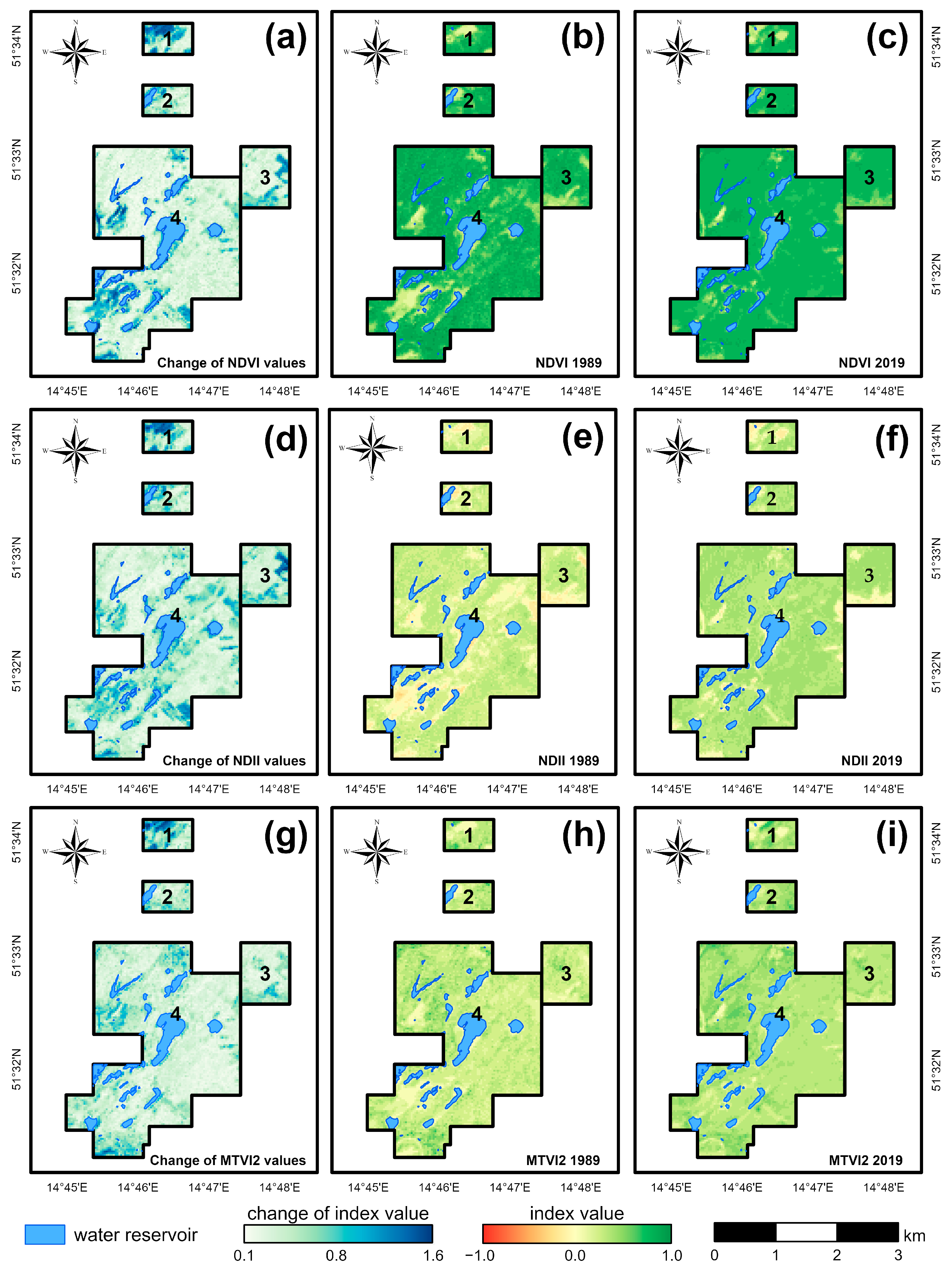
• identification of sites with significant flora changes;
• testing GIS-based methodology to analyze the relationship between the condition of vegetation and the potential topographical and mining driving factors.

A unique aspect of the research arises from the fact that the study area was subjected to long-term, combined, underground, and open-cast mining in complex glaciotectonic conditions. The mineral extraction ended in the 70s of the 20th Century, and the area now constitutes a part of the UNESCO Global Geopark “Muskau Arch.” The background of this study also lies in the fact that numerous secondary effects of former mining activity, such as sinkholes, subsidence basins leading to localized waterlogging, and waste heap weathering have been observed there. Up to this date only limited in situ investigations have been conducted in the study area [45,46,47,48,49], and our work is the first research that utilizes remotely sensed multispectral satellite imagery and GIS. Time-series analysis (1989–2019) of the following vegetation indices: Normalized Difference Vegetation Index (NDVI), Modified Triangular Vegetation Index-Improved (MTVI2), and Normalized Difference Infrared Index (NDII) was applied to study vegetation condition in the post-mining period. Then we used algebra and multivariate, spatially weighted regression methods to identify zones of significant changes of flora condition and to analyze the statistically significant driving factors behind these changes. The proposed methodology can be applied to a long-term analysis of vegetation condition in other lignite mining and post-mining areas with similar spatial and temporal characteristics.

2. Study Area

The former mining site “Babina” is located in Western Poland, close to the border with Germany between 14°43′E and 14°51′E and 51°31′N and 51°42′N. In terms of geomorphology, it is located in the eastern fragment of the glaciotectonic structure called the Muskau Arch, which is characterized by a horseshoe-like shape, open towards the North. The Muskau Arch is divided by the Nysa Łużycka river that constitutes the border between Poland and Germany. The arch was formed probably during the South Polish (Elsterian) Glaciations, but its shape was remodeled during the succeeding glacial periods (Figure 1) [50].

The analyzed geomorphological structure is located within the Paleozoic platform made up of three structural levels: the Precambrian crystalline bedrock, folded Caledonian-Hercynian Paleozoic formations and the Zechstein-Mesozoic-Cenozoic platform cover. The latter is characterized by a wealth of mineral resources, including lignite and construction clays [51].

The glacial processes led to the exposure of lignite deposits, which contributed to the beginning of mining operations within the whole of the Muskau Arch. In the now Polish part of this structure, mining began in the second half of the 19th Century. The “Babina” mine started its operation in 1921 and was the largest one in the area. Both underground and open-cast mining methods were used due to the complexity of the folded lignite seams [52]. These unfavorable geological-mining conditions had also been the cause of the closing of the operation in 1973 due to economic reasons. Restoration of the post-mining area, aimed at the flooding of the old open pits and reforestation of the ground, started soon afterward [53]. Presently, the dominant plant species are pine forests, as well as alder and riparian forests. In total, over 1500 species of vascular vegetation, including ruderal and replacement plants, have been classified in the post-mining area [45]. The region was declared a Global UNESCO Geopark in 2015 because of the unique anthropogenic landscape that includes anthropogenic lakes with a low pH level and high Fe content, waste heaps and relics of mining infrastructure, as well as geological settings (valleys formed by glacial erosion, hills made of glacial erratic boulders, sands, and gravels, and gizers—ditches formed by weathering and subsiding of exposed lignite outcrops) [46,52,53].

The research presented in this paper has been conducted in the “Pustków” mining field located in the southern part of the “Babina” mine (Figure 1). The four specific study sites (test fields) of 877.54 ha, where the analysis of the vegetation state in 1989–2019 was carried out, coincide with the extent of the available historical, geological, and mining maps, describing the done mining operation in the research area.

3. Materials and Methods

3.1. Geospatial Data

In this study, the multispectral Landsat TM/ETM+/OLI images (Landsat Collection Level-1), downloaded from the EarthExplorer platform (https://earthexplorer.usgs.gov/ (accessed on 12 May 2021)), were used to analyze the changes in the vegetation condition in a post mining area in the 1989-2019 period. Overall, 30 images, registered in the period characterized by similar features of flora located in the western Poland (from May to the end of September), were used. The number of available images was reduced by the criterion of a maximum cloud cover, set at the 10% level.

Table A1. Satellite images used for the analysis of changes in the flora condition in the research area in the period 1989–2019 (own study based on website: https://www.usgs.gov/landsat-missions (accessed on 12 May 2021)).

Mission	Sensor Name	Duration of Mission	Number of Spectral Bands	Spectral Range [µm]	Spatial Resolution [m]	Date of the Acquired Image
Landsat 5	Thematic Mapper (TM)	03.1984–06.2013	7	0.45–12.5	visible light, infrared bands: 30 m thermal band: 120 m	18.09.1989, 04.08.1990, 07.08.1991, 10.09.1992, 08.05.1993, 31.08.1994, 18.08.1995, 20.08.1996, 01.09.1997, 10.08.1998, 14.09.1999, 11.05.2000, 14.05.2001, 18.06.2002, 25.09.2003, 10.08.2004, 29.08.2005, 26.09.2006, 19.08.2007, 29.07.2008, 24.08.2009, 12.09.2010, 24.09.2011
Landsat 7	Enhanced Thematic Mapper Plus (ETM+)	04.1999–at present	8	0.45–12.5	visible light, infrared bands: 30 m thermal band: 60 m panchromatic band: 15 m	20.05.2012
Landsat 8	Operational Land Imager (OLI)	02.2013—at present	11	0.43—12.5	visible light, infrared bands: 30 m panchromatic band: 15 m thermal bands: 100 m	15.05.2013, 07.09.2014, 19.09.2015, 12.09.2016, 30.08.2017, 17.08.2018, 21.09.2019

(Appendix A) shows the dates of the acquired remote sensing satellite images, as well as the basic information about the sensors which registered this data.

In addition to the satellite imagery, the following data were used:

• 67 archival geological and mining maps were drawn at the 1:1000 scale between 1956–1973, obtained from the State Mining Authority and listed in Table S1 (Supplementary Materials);
• vector data from the Database of Topographical Objects (scale 1: 10,000) representing the location of water reservoirs in the research area and available from [54];
• Digital Elevation Model (DEM) (1 m resolution) obtained from aerial laser scanning performed in 2020 and available from [55];
• German Topographical Map—Messtischblatt drawn at the 1:25,000 scale and representing the study area as it was in 1911;
• vector data representing the extent of the glaciotectonic structures and documented locations of gizers in the area, developed by [56];
• vector data representing boundaries of mineral deposits in Poland available from [57];
• Hydrogeological Map of Poland from the year 2006 and drawn at scale 1:50,000 [58];
• archival meteorological data (precipitation and air temperature) for the 1989–2019 period (corresponding to the months of satellite imagery acquisitions), obtained from [59].

The data were used to develop a GIS database of potential driving (causative) factors behind the observed changes of vegetation condition. The database consisted of independent variables characterizing former mining activity and geological and topographical conditions applied in the tested multivariate spatial regression models. The meteorological data were used to test if the calculated statistics of the analyzed spectral indices were related to the atmosphere conditions.

3.2. Pre-Processing of Satellite Data

The acquired satellite data were subjected to processes aimed at standardizing the images registered by various sensors in different weather and lighting conditions. In the first stage, the radiometric Digital Number (DN) values were converted to the values of the registered ${\mathrm{L}}_{\mathrm{SAT}}$ radiance, using the following Equation (1):

$${\mathrm{L}}_{\mathrm{SAT}}={\mathrm{c}}_0+{\mathrm{c}}_1\ast \mathrm{DN},$$

(1)

where: ${\mathrm{c}}_0$ and ${\mathrm{c}}_1$ are the calibration constants, stored in the metadata, for a specific type of sensor and spectral band, called the offset and gain, respectively [60].

In the next step, the atmospheric correction of the images was performed, considering:

• the average terrain height of the former mining field (100 m a.s.l.);
• atmosphere model—in this study, based on the image registration date, models with a water vapor content of 2.08 $\mathrm{g}/{\mathrm{cm}}^2$ or 2.92 $\mathrm{g}/{\mathrm{cm}}^2$and an average air temperature of 14 or 21 °C were used (Sub-Arctic Summer and Mid-Latitude Summer models, respectively);
• aerosol model—in the analyzed case, a model dedicated to a slightly polluted and non-urbanized areas was selected.

The atmospheric correction of the image registered by the ETM+ sensor was preceded by the removal of the scan line error, using an algorithm based on the triangulation (the Scan Line Corrector was damaged in June 2003, resulting in white lines covering the images) [61].

All of these operations were performed in the ENVI 5.6. software, licensed to the Wroclaw University of Science and Technology, using the Raster Management, FLAASH and Radiometric Correction modules.

3.3. Remote Sensing Vegetation Indices

Pre-processed images were used to calculate the following vegetation indices in ENVI 5.6. software:

• Normalized Difference Vegetation Index (NDVI)—that is a combination of red and near-infrared bands, the spectral ranges in which the highest absorption and reflection of solar radiation by vegetation are observed, respectively [62]. This index enables the identification of flora among other forms of land cover and the general assessment of its condition and is given by the formula (2):

  $$\mathrm{NDVI}=\frac{\mathrm{NIR}-\mathrm{RED}}{\mathrm{NIR}+\mathrm{RED}} ,$$

  (2)

  where: NIR and RED are the spectral reflectance values in the near-infrared and red bands, respectively [17].

The NDVI index takes values between −1 and 1, with negative values indicating non-vegetated areas, values from the 0.2–0.8 interval being characteristic for areas covered with green plants, and index values exceeding 0.8 indicating dense and healthy plant cover [63];

2.

Normalized Difference Infrared Index (NDII)—developed by Hardisky et al. [64] using the reflectance value in the near and short infrared bands. NDII enables to assess the water content of vegetation, and it is given by the formula (3):

$$\mathrm{NDII}=\frac{\mathrm{NIR}-\mathrm{SWIR}1}{\mathrm{NIR}+\mathrm{SWIR}1},$$

(3)

where: SWIR1 is the spectral reflectance value in the short infrared band.

NDII, similarly to the NDVI index, takes values from −1 to 1, with negative values indicating a deficiency of water in the vegetation [65,66];

3.

Modified Triangular Vegetation Index—Improved (MTVI2)—spectral bands combination developed by Haboudane et al. [67], used for the estimation of leaf area index (LAI), with the following formula (4):

$$\mathrm{MTVI}2=\frac{1.5\ast \left[1.2\ast \left({\mathrm{R}}_{800}-{\mathrm{R}}_{550}\right)-2.5\ast ({\mathrm{R}}_{670}-{\mathrm{R}}_{550}\right)]}{\sqrt{{\left(2{\ast \mathrm{R}}_{800}+1\right)}^2-(6{\ast \mathrm{R}}_{800}-5\ast \sqrt{{\mathrm{R}}_{670}}})-0.5} ,$$

(4)

where: ${\mathrm{R}}_{800}$, ${\mathrm{R}}_{550},$and ${\mathrm{R}}_{670}$are the spectral reflectance values for the wavelengths of 800 nm, 550 nm, and 670 nm, respectively.

The MTVI2 index is very sensitive to changes in leaves and canopy structures, a decrease in the index value indicates a lower ratio of the leaf area to the ground area, whereas an increase indicates the growth of the tree canopy. It is resistant to the influence of soils and changes in the concentration of photosynthetic pigments [67].

3.4. Spatial Statistics and Multivariate Weighted Spatial Regression

The map algebra local functions (cell statistics) implemented in the ESRI ArcGIS Pro 2.8.0 software were used to determine the range of changes in vegetation indices values for each pixel of the research area in the 1989–2019 period and identify significant changes in plant cover condition.

Then, multivariate spatial regression methods were used to analyze the relationship between the identified vegetation changes over a 30-year period (spectral indices used as dependent variables) and the potential mining, geological, and topographical driving factors (independent explanatory variables in the models). First, the global and then local spatial regression methods have been applied to determine the potential relationship between these factors and flora condition represented by the change of indices.

Due to the spatial heterogeneity of the variables representing the area of the combined, underground and open-cast mining identified in the constructed global regression models, the weighted spatial regression approach has been subsequently applied. The general formula of a Geographically Weighted Regression (GWR) model is given by (5):

$${\mathrm{y}}_{\mathrm{i}}\left(\mathrm{u}\right)={\mathsf{\beta }}_{0\mathrm{i}}\left(\mathrm{u}\right)+{\mathsf{\beta }}_{1\mathrm{i}}\left(\mathrm{u}\right){\ast \mathrm{x}}_1+\cdots +{\mathsf{\beta }}_{\mathrm{ni}}\left(\mathrm{u}\right){\ast \mathrm{x}}_{\mathrm{n}}+ {\mathsf{\epsilon }}_{\mathrm{i}},$$

(5)

where: ${\mathrm{x}}_1$, ${\mathrm{x}}_2$,…, ${\mathrm{x}}_{\mathrm{n}}$—are the independent variables, ${\mathsf{\beta }}_{0\mathrm{i}}\left(\mathrm{u}\right)$, ${\mathsf{\beta }}_{1\mathrm{i}}\left(\mathrm{u}\right)$, …, ${\mathsf{\beta }}_{\mathrm{ni}}\left(\mathrm{u}\right)$ are the coefficients describing the relationship between the location u and a particular independent variable, characteristic feature of each location, ${\mathsf{\epsilon }}_{\mathrm{i}}$—random error [68].

The theory behind multivariate spatial regression has been described in [69,70]. The important aspect of the method is the construction of local models based on the neighborhood matrix with the use of a weighting function. Weights in the matrix depend on the distance between the given location and its neighbors [71].

The dependent variables for the regression models were the spatial statistics calculated for the NDVI, NDII, and MTVI2 indices. The considered, independent (explanatory) variables describing the former mining activity, as well as the geological and topographic conditions of the research area, were:

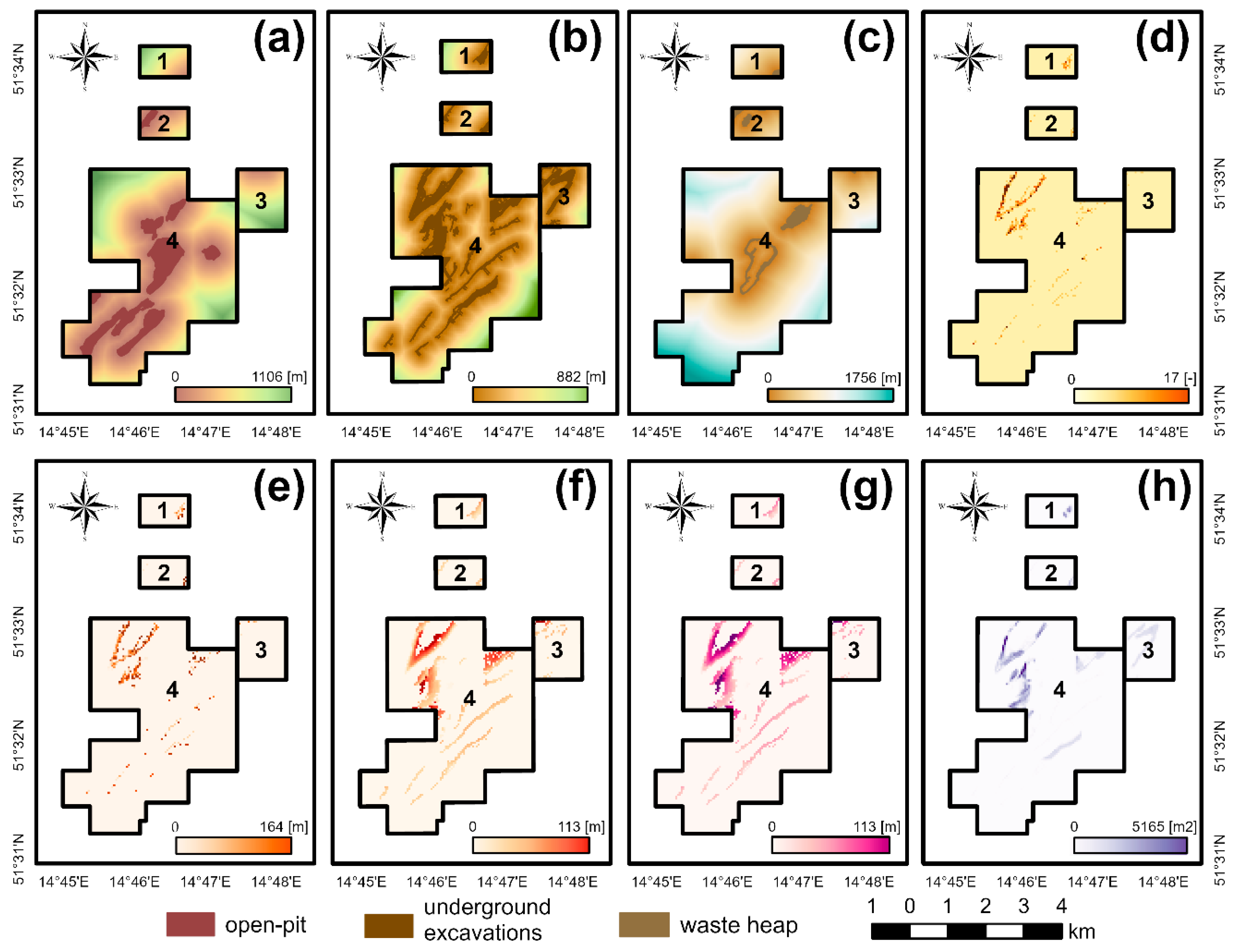
• mining factors: number of shafts per reference unit area, average and minimum depth of the underground excavations, the average depth of the mining shafts, distance from former open pits, distance from the underground workings, distance from the mining waste heaps, area of the underground mining excavations per reference unit area;
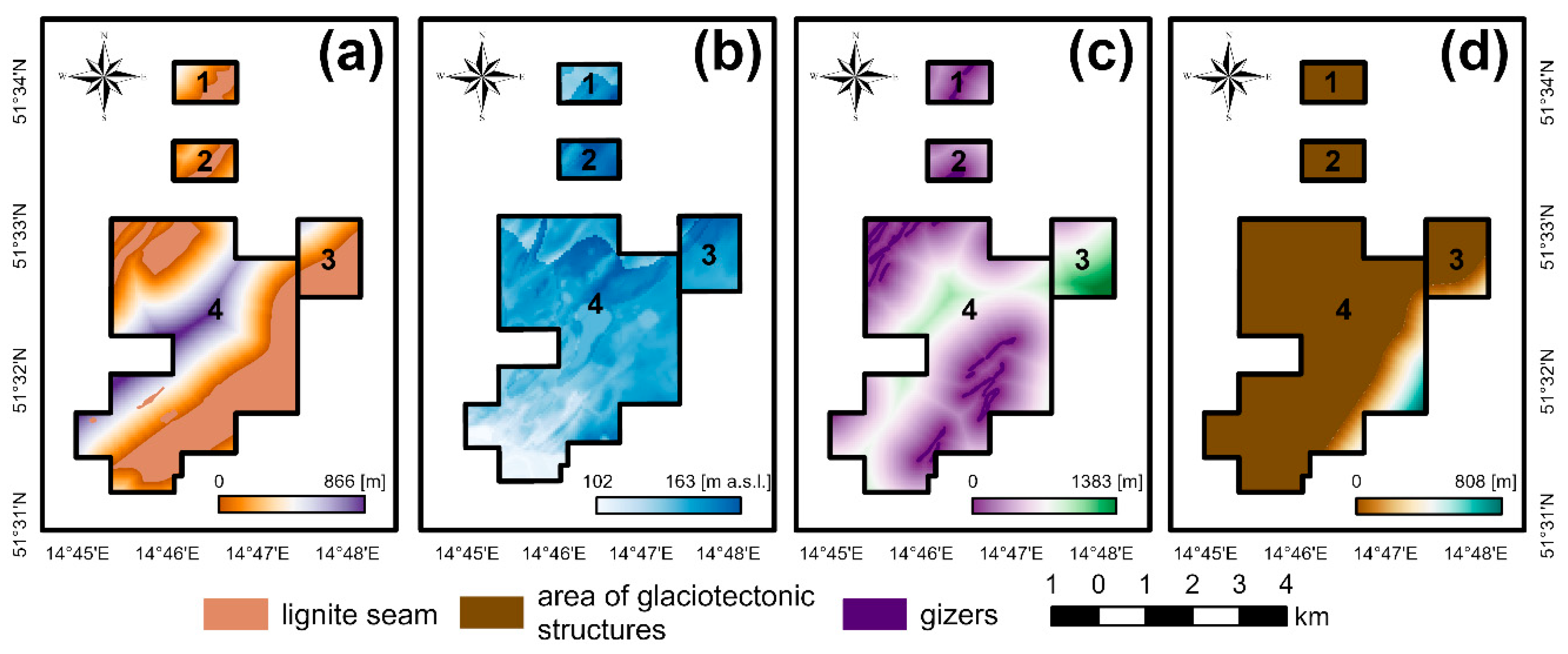
• geological factors: distance from lignite seams, distance from gizers, groundwater table elevation, distance from the boundary of glaciotectonic changes;
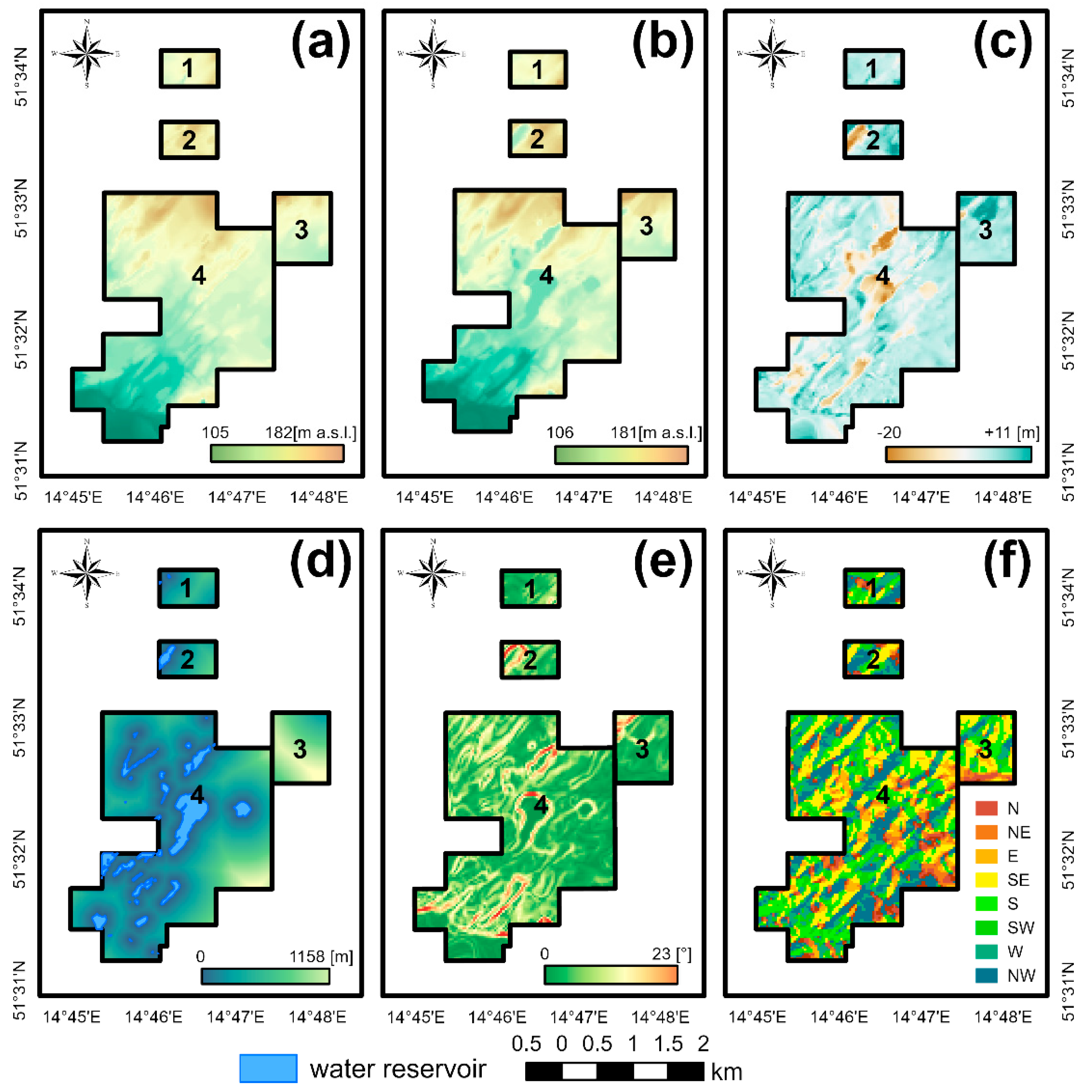
• topographic factors: DEM (as in the year 2020), DEM (as in the year 1911), DEM of Difference (2020–1911), slope and aspect of the terrain, and distance from the anthropogenic lakes.

All of the variables were represented by raster data with a cell size of 30 m × 30 m and have the same spatial extent (S 5 707 725 m, N 5 714 745 m, E 487 035 m, W 482 635 m) and coordinate system (WGS 84 UTM zone 33). The detailed information on the source and processing of data to prepare spatial representation of independent variables can be found in Table S2 (Supplementary Materials).

The construction and testing of spatial regression models were preceded by exploratory data and correlation analysis of the independent variables (with Layer Stack and Band Statistics tools in ENVI 5.6. software) in order to eliminate the collinear factors (global collinearity).

The evaluation of the global and the local multivariate spatial regression models was performed based on their statistics: regression residuals, the spatial distribution of the residuals, Akaike’s information criterion (AICc), as well as the value of adj${\mathrm{R}}^2$coefficient (square of Pearson’s linear correlation), and the strength of the local coefficients [72].

These tasks were performed in the ArcGIS Pro 2.8.0 software, licensed to the Wroclaw University of Science and Technology.

4. Results

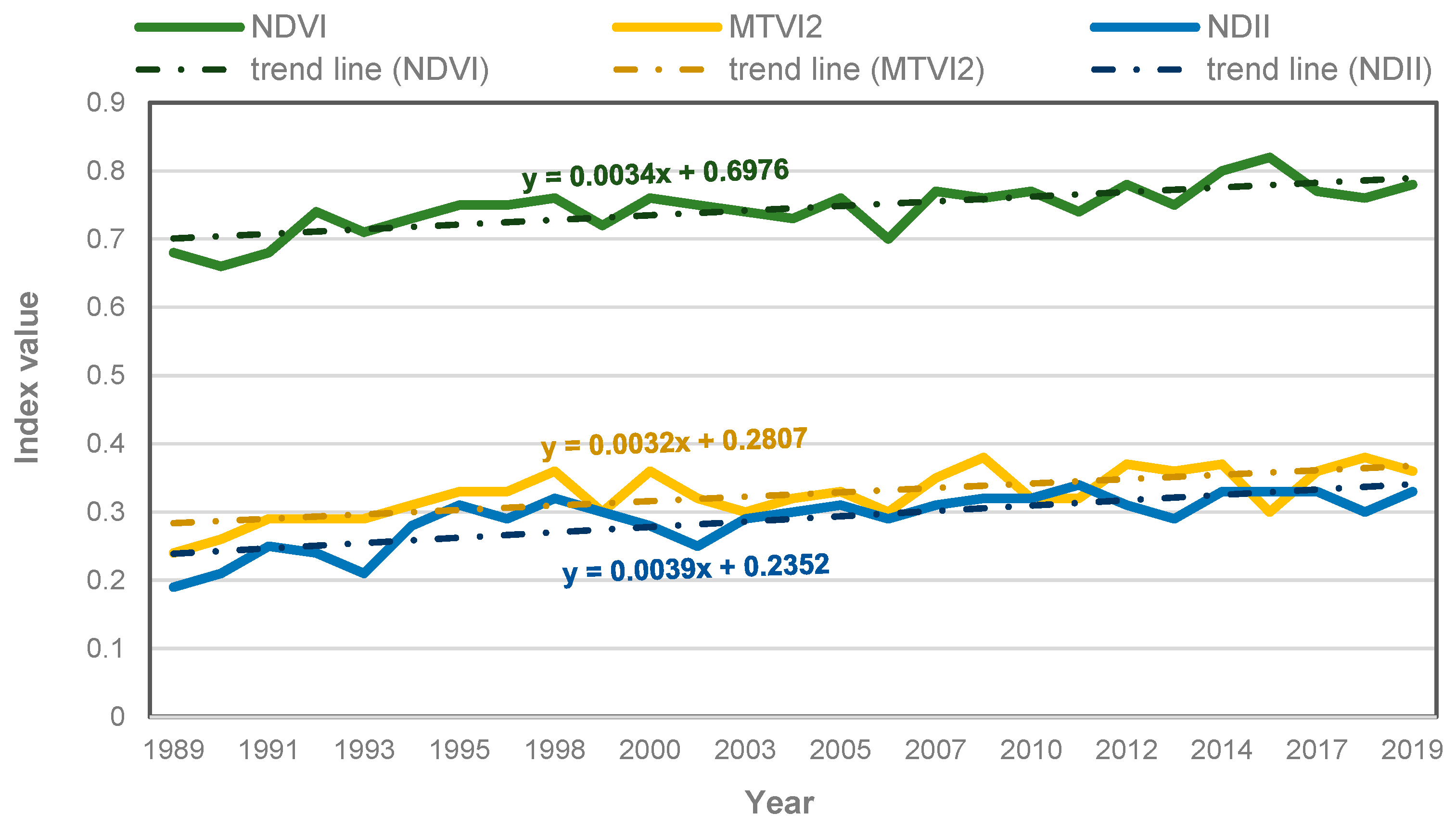
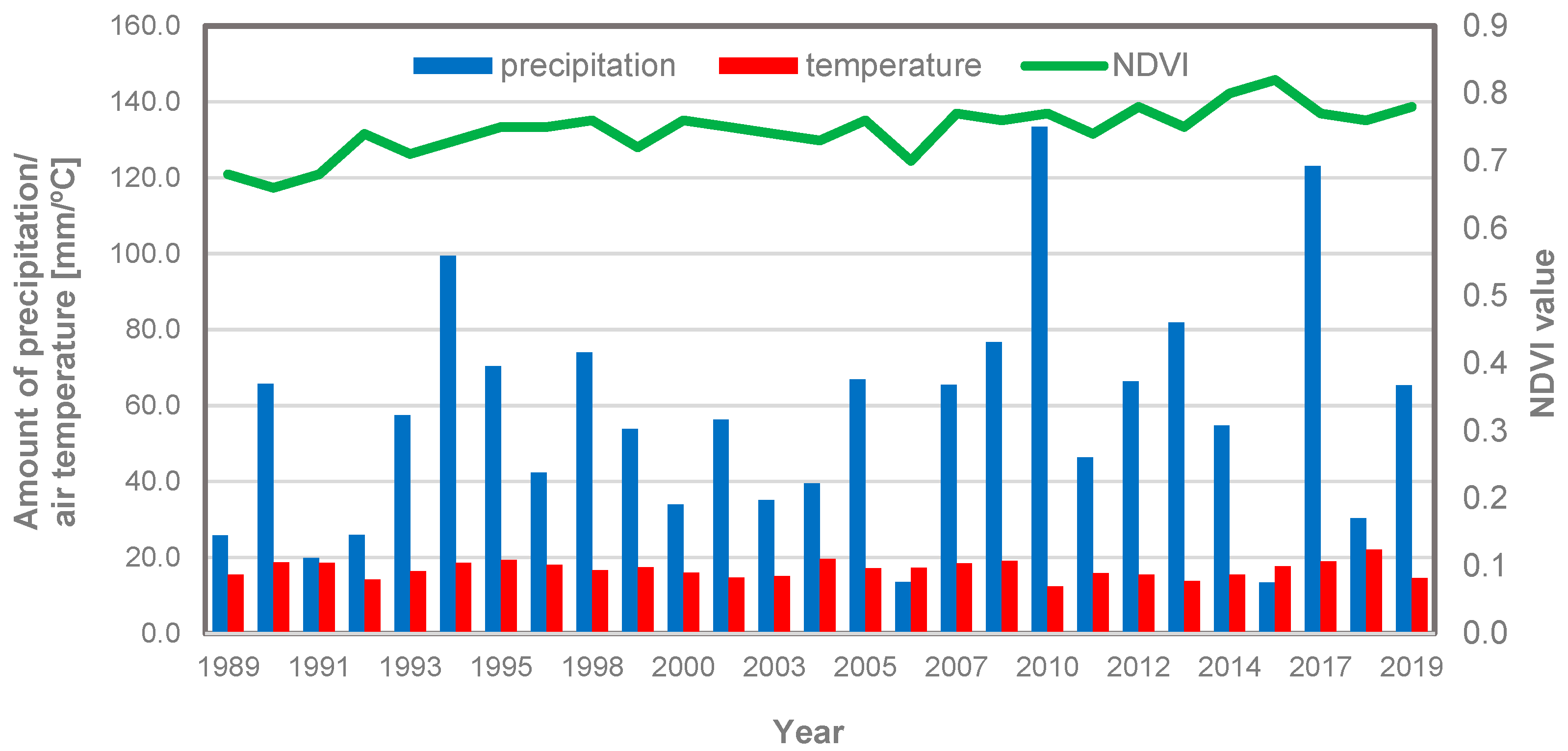
4.1. Vegetation General Condition in the 1989–2019 Period

The first stage of the research was aimed at the analysis of the average annual values of the NDVI, NDII, and MTVI2 indices. As shown in Figure 2, an increase in the values of all of the analyzed indices was observed in the 1989–2019 period (the average values of all spectral indices increased by approximately 0.15 over the 30-years period). The values for 1997, 2002, 2008, and 2015 were not analyzed as the images available for these years did not meet the minimum cloud cover criterion.

The NDVI index had the lowest average value in 1990 (0.66) and the highest one in 2016 (0.82). The highest average values of the NDII and MTVI2 indices were observed in 2011 and 2018 respectively (0.34 and 0.38), while the lowest ones were noticed in 1989 (0.19 and 0.24, respectively).

The trend lines representing general temporal changes of the analyzed indices are similar (Figure 2). The strength of the relationships between the NDVI, NDII, and MTVI2 was determined with the Pearson correlation coefficients, calculated for each possible combination of these indices. The results indicate that the NDII and NDVI are highly correlated (correlation coefficient of 0.80), while the MTVI2 and NDII, as well as the MTVI2 and NDVI, are characterized by an even stronger linear relationship (correlation coefficients of 0.83 and 0.82, respectively). Thus, a change in the value of one spectral index corresponds to a change in the value of the other indices. All of the determined correlation coefficients are positive [73].

This indicates a gradual improvement in the general condition of vegetation in the post-mining area, increased water content in plants, and growth of the tree canopies (larger area and density of leaves). In the analyzed period, only the results for 1993, 2002, and 2006 showed slight discrepancies from the general trend.

In order to verify whether the identified changes in vegetation conditions have been influenced by extreme meteorological conditions (drought periods or heavy precipitation), the results were compared with the average air temperature and precipitation for the 1989-2019 period. As shown in Figure 3, precipitation significantly higher than the average for the analyzed period was observed in 1994, 2010, and 2017 with an average precipitation of 99.4, 133.2, and 123.1 mm, respectively, and with dry periods in 1989, 1991–1992, and 2016. The average amount of precipitation for the 1989-2019 period was 56.9 mm. Thus, it can be assumed that the variation of meteorological parameters did not cause any increase or decrease in the analyzed indices. The identified positive changes in the plant cover general condition are part of a trend that has not been disturbed by extreme meteorological conditions (the correlation coefficients between the NDVI index value and the average air temperature and precipitation amount were −0.14 and 0.24, respectively).

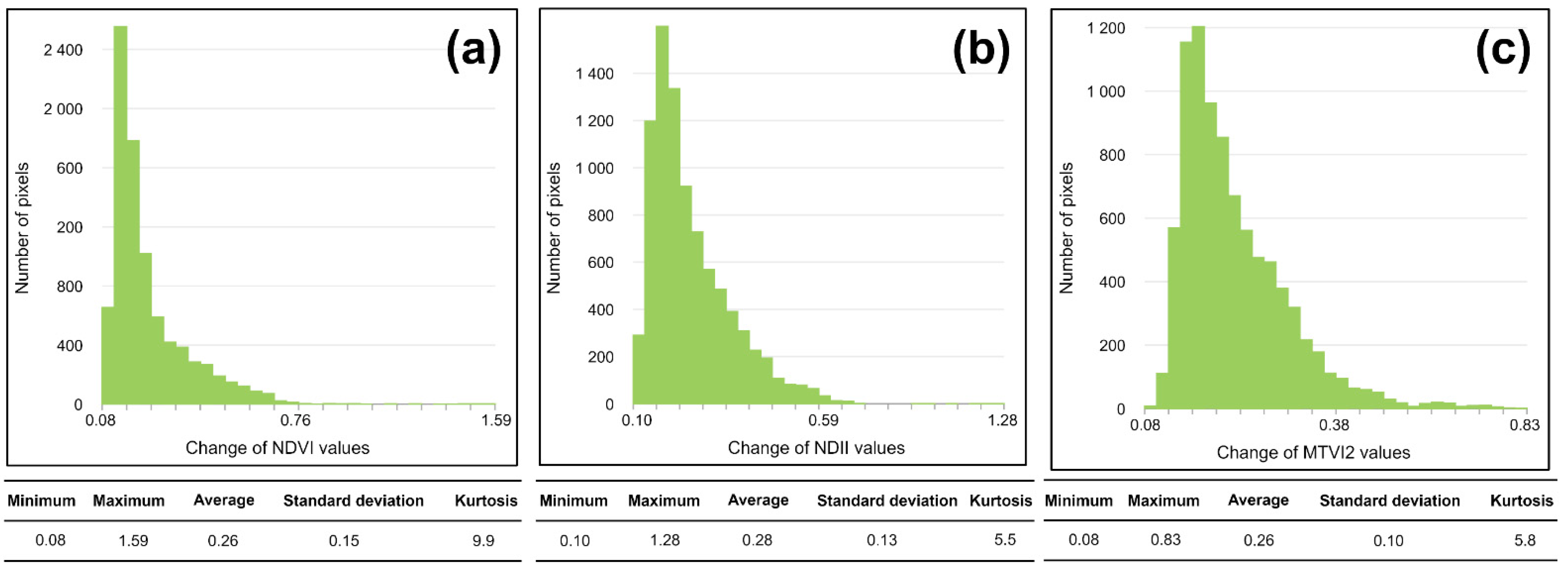
4.2. Statistical Analysis of Dependent Variables

The raster range cell spatial statistic, determined for the NDVI index, is characterized by a log-normal distribution, and its values are in the 0.1–1.6 range (Figure 4a). The average value of NDVI change is equal to 0.26. The smallest changes of the NDVI index value in the 1989–2019 period, less than 0.2, were observed in the eastern parts of test fields no. 1 and 2, in the western part of test field no. 3, as well as in the northwestern and eastern parts of the test field no. 4 (Figure 5a). The greatest changes occurred in the northwestern part of field no. 1, in the western part of field no. 2, in the eastern and southern parts of field no. 3, in the western part of field no. 4, and along the shorelines of anthropogenic water reservoirs (changes in index values higher than 0.6). The greatest changes of the NDVI values, except for the northwestern part of test field no. 1, were positive (increase in the index value over a period of 30 years at the level of 0.2–0.6), which was confirmed by analysis of distribution of index values in 1989 and 2019 (Figure 5b,c).

The statistic, determined for the NDII, is characterized by a range of values (0.1–1.3), similar to the NDVI distribution (log-normal) and the average change in time (0.28) (Figure 4b). Analysis of the statistic value variability within the test fields indicates that the regions of the largest and the smallest changes of the NDII value overlap with the boundaries of the areas identified for the NDVI index (Figure 5d). Significant negative changes of NDII were observed in the northwestern part of test field no. 1, as in the case of NDVI (Figure 5e,f).

The statistic, determined for the MTVI2 index, has the smallest range of values (0.1–0.8) and a log-normal distribution. The average variability of MTVI2 value within the cells of the research area is equal to 0.26 (Figure 4c). The distribution of this statistic in the test fields is different than in the case of the NDVI and NDII. The changes of the MTVI2, observed in most of the areas of interest, do not exceed the value of 0.4. The greater variability of these index values was noticed only in the northwestern part of test field no. 1 and in the southern parts of test fields no. 3 and 4 (Figure 5g). The areas of the greatest changes in the MTVI2 index, apart from the northwestern part of test field no. 1, were characterized by an increase in leaf area and denser tree canopies in the period of 1989-2019 (Figure 5h,i).

Based on the spatial distribution of the range of NDVI, NDII, and MTVI2 values, we identified the zones of the greatest change in the plant cover condition. These are the northwestern part of test field no. 1, the western part of test field no. 2, the eastern part of test field no. 3, the western part of test field no. 4, as well as the vicinities of the anthropogenic water reservoirs (in the vicinity of anthropogenic lakes, statistics determined for NDVI and NDII indices are characterized by values greater than 1.0, which indicates the change in the area of water bodies).

4.3. Independent Variables

4.3.1. Mining Factors

The former open pits were located in fields no. 2 and 4. These are now anthropogenic lakes. The spatial distribution of the distance to former open pits is presented in Figure 6a.

Underground mining was conducted in each of the test fields, most intensively in test field no. 4. Distance to these sites is presented in Figure 6b.

Mining waste heaps are located in the southeastern part of test field no. 1, in the northwestern part of test field no. 2, in the northeastern part of test field no. 4, and along the shoreline of the largest lake in the middle of the test field no. 4 (Figure 6c).

Vertical mining excavations (underground ore passes, shafts) are associated with the underground mining sites. Their number is the highest in test field no. 4. The distribution of their number per reference unit (pixel) is shown in Figure 6d.

The average depth of vertical excavations in the analyzed research area varies from 20 to 40 m b.s.l. (Figure 6e). The deepest mining shafts (140 to 160 m b.s.l.) were located in the southeastern part of test field no. 2 and in the northwestern and northern parts of test field no. 4.

The average depth of the underground production levels varies from 40 m to over 100 m b.s.l. located in test fields no. 3 and 4. The spatial distribution is presented in Figure 6f. Analogous distribution of values in the study area is observed for the variable “minimum depth of the underground excavations” (Figure 6g).

The area of the underground mining excavations was calculated as the sum of all underground levels in a given reference pixel. The distribution of this variable ranges from less than 300 ${\mathrm{m}}^2$ in sites located in test fields no. 2 and 3 to over 4200 ${\mathrm{m}}^2$ in the northeastern part of test field no. 4 (Figure 6h).

4.3.2. Geological Factors

The lignite seams in the research area are a scale-like form extending along the SW—NE direction. The map of distance from documented deposits is presented in Figure 7a.

The groundwater table level variable ranges from 130 to 140 m a.s.l. and its spatial distribution is shown in Figure 7b. At this point, it is worth emphasizing that there is no aquifer within anthropogenic reservoirs, thus the values of the terrain height (as in the year 2020) have been assigned to the pixels representing post-mining lakes.

Weathering ditches, locally called gizers, are exposed lignite formations and extend along the SW–NE direction. They are present in all study sites, except test field no. 3 (Figure 7c).

Glaciotectonic structures are located in most of the area of interest. The boundary runs along the southeastern part of test fields no. 3 and 4 (Figure 7d).

4.3.3. Topographic Factors

The relief of the terrain in the area prior to mining was reconstructed through the digitization of the 1911 topographic map. The southwestern part of test field no. 4, close to the Nysa Łużycka river valley, had the lowest elevation (less than 130 m a.s.l.). The sites are located in the eastern part of test field no. 1, in the central part of test field no. 2 and in the northern parts of test fields nos. 3 and 4 had the highest elevation (Figure 8a).

In the period of 109 years, the area changed significantly. For example, a decrease in the terrain height, more than 15 m, was observed in fields nos. 2 and 4. The Digital Elevation Model (DEM) in 2020 is shown in Figure 8b.

The map of a variable representing DEM of Difference between the above two DEMs is presented in Figure 8c. The elevation changes are the result of terrain subsidence over underground mines, the development of open pits subsequently filled with waste materials, the development of waste heaps, and other anthropogenic activity.

Post-mining water reservoirs are present in the entire AOI with the exception of test field no. 3. The variable representing the distance from anthropogenic lakes is presented in Figure 8d.

The slope variable is shown in Figure 8e. Over 80% of the area is characterized by slope values lower than 2°. Higher slope values (10–22°) are associated with the shorelines of anthropogenic lakes and mining waste heaps.

The most common terrain aspect classes include SW, SE, and NW directions. The northern aspect is the least frequent one (Figure 8f).

4.4. Correlation Analysis of Independent Variables

The results of the correlation analysis between all the considered variables have been presented in the form of a matrix (Figure S1 in Supplementary Materials). Significant, very strong correlations with Pearson coefficient values of 0.86 or above have been identified for the following pairs of variables: slope and aspect of the terrain, DEM in 2020 and in 1911, average and minimum depth of underground excavations, distance from gizers, and the boundary of the glaciotectonically transformed area. Strong correlations exist between distance from open pits and distance from underground mining areas, distance from underground mining areas and distance from waste heaps, number of mining shafts in reference unit, and the average depth of mining shafts.

Taking into account the results of both the correlation analysis and exploratory data analysis for all potential combinations of variables in global regression models and their Variance Inflation Factor (VIF) values [74], the following independent variables were selected as potential driving factors: distance from the anthropogenic lakes, DEM (2020), DEM of Difference (2020–1911), distance from the lignite seams, distance from former open pits, distance from the underground workings, distance from waste heaps, distance from gizers, as well as the aspect of the terrain.

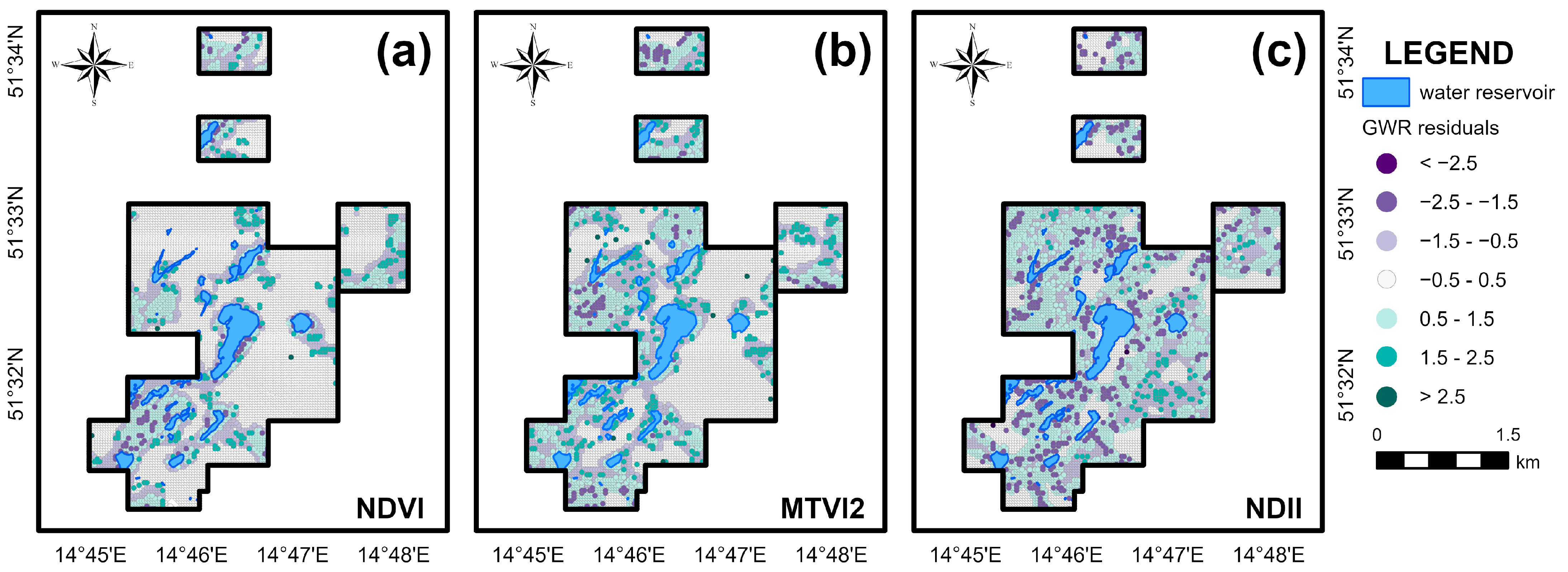
4.5. Multivariate Weighted Spatial Regression Models

The development of the multivariate weighted spatial regression models was preceded by the reclassification of the values of the dependent variables that did not have a normal distribution. The reclassified data take the values of 0 or 1, denoting significant or insignificant changes in the spectral indices’ values in the period of 1989-2019. The threshold values for significant changes were determined from the distribution of the indices (histograms in Figure 4) and were above 0.3, 0.4, and 0.6 for MTVI2, NDVI, and NDII, respectively.

The logistic (binary) regression model and neighborhood search (bandwidth) algorithm, based on the minimum value of AICc, were selected to determine the extent of kernel, in accordance with the spatial regression calculation theory for binary data and regular space tessellation.

The best-fitting spatial regression models demonstrated that independent variables (listed in Table S2) explain between 48% (${\mathrm{adjR}}^2$for NDII model) and 62% (${\mathrm{adjR}}^2$ for the NDVI model) of changes in the values of the analyzed vegetation indices in the period of 1989–2019. The values of the Akaike Information Criterion (AICc) for the obtained regression models, for the NDVI, NDII, and MTVI2 indices, were equal to 4362.7, 7612.0, and 6245.4, respectively.

The distribution of residuals for the spatial regression models indicated that the areas of the greatest underestimation and overestimation of the model, developed for the NDVI index, were observed in the southwestern part of test field no. 1, in the western part of test field no. 2, in the southern and eastern parts of test field no. 3, in the western part of test field no. 4, as well as along the shorelines of anthropogenic lakes (Figure 9a). In the remaining parts of the analyzed area the model performed well. The distribution of residuals from the MTVI2 model is similar (Figure 9b). However, the obtained residuals are greater. The residuals for the NDII model are characterized by a greater discrepancy from the observed values. The areas of underestimation and overestimation cover the majority of test field no. 4, the eastern parts of test field no. 1 and 2, as well as the central part of test field no. 3 (Figure 9c).

The residuals from the regression models developed for the NDII and MTVI2 indices are characterized by a bimodal distribution.

The character and strength of the relationship between the independent variables and the plant cover condition changes represented by the reclassified values of the spectral indices are given by the local coefficient values and their sign determined for each reference unit.

Table 1. Coefficients of the independent variables.

Independent Variables	NDVI				NDII				MTVI2
	Min	Max	Mean	Std	Min	Max	Mean	Std	Min	Max	Mean	Std
Distance from the anthropogenic lakes	−7.98	0.25	−0.05	0.29	−0.35	0.58	−0.01	0.05	−4.04	1.35	−0.03	0.17
DEM (2020)	−4.71	3.02	−0.39	0.24	−3.29	4.74	−0.08	0.60	−9.43	12.20	−0.17	0.99
DEM of Difference (2020–1911)	−19.12	5.69	−0.13	0.72	−4.13	3.24	−0.05	0.53	−20.33	5.10	−0.07	1.09
Distance from the lignite seams	−0.72	0.66	0.00	0.05	−0.49	0.35	0.00	0.05	−2.27	0.89	−0.01	0.10
Distance from former open pits	−1.13	7.93	0.02	0.27	−0.78	0.40	0.00	0.06	−1.99	3.39	0.01	0.15
Distance from the underground workings	−0.12	2.35	0.02	0.13	−0.21	0.75	0.00	0.04	−0.15	1.50	0.02	0.08
Distance from the waste heaps	−0.14	0.66	0.01	0.04	−0.20	0.84	0.01	0.05	−0.58	1.39	0.00	0.04
Distance from gizers	−0.74	0.50	0.00	0.07	−0.61	0.41	0.01	0.05	−0.77	0.32	0.00	0.05
Aspect	−0.06	0.19	0.00	0.01	−0.11	0.02	0.00	0.01	−0.28	0.13	0.00	0.01

contains basic information on the coefficients assigned to the individual independent variables in the GWR models.

Table 2. GWR models: identification of areas of clearly positive influence of the independent variables on the vegetation indices (based on Figures S2–S4).

Independent Variable *	The Area of Positive Influence of the Independent Variable
	NDVI	NDII	MTVI2
DEM (2020)	the NE part of the test field no. 4	the NE and SW parts of the test field no. 4	the NE and SE parts of the test field no. 4
DEM of Difference (2020–1911)	the NW, SW and SE parts of the test field no. 4	the NW part of the test field no. 1	the NW part of the test field no. 1, southern part of the test field no. 3, SW and SE parts of the test field no 4.
Distance from lignite seams	not identified	not identified	not identified
Distance from former open pits	The SE part of the test field no. 4	not identified	the SE part of the test field no. 4
Distance from underground workings	the NW part of the test field no. 4	not identified	not identified

* The coefficient values for distance from anthropogenic lakes, distance from waste heaps, distance from gizers, as well as for aspect of the terrain in each of the developed GWR model ranged from 0 to 1.5.

and

Table 3. GWR models: identification of areas of clearly negative influence of the independent variables on the vegetation indices (based on Figures S2–S4).

Independent Variable *	The Area of Negative Influence of the Independent Variable
	NDVI	NDII	MTVI2
Distance from anthropogenic lakes	the NW and SE parts of the test field no. 4	not identified	the SE part of the test field no. 4
DEM (2020)	the NE and SW parts of the test field no. 3, SW and SE parts of the test field no. 4	the NW part of the test field no. 1, SE part of the test field no. 3, eastern part of the test field no. 4	the NW part of the test field no. 1, the southern part of the test field no. 3, eastern and SW parts of the test field no. 4
DEM of Difference (2020–1911)	the NE and SE parts of the test field no. 4	the southern part of the test field no. 3 and NE part of the test field no. 4	the southern part of the test field no. 3 and eastern part of the test field no. 4
Distance from lignite seams	not identified	not identified	the SE part of the test field no. 4
Distance from former open pits	not identified	not identified	the SE part of the test field no. 4

* The coefficient values for distance from underground workings, distance from waste heaps, distance from gizers, as well as for aspect of the terrain in each of the developed GWR models ranged from −1.5 to 0.

describe the areas where the influence of a given independent variable on changes in the analyzed vegetation indices is positive (the coefficient value is above 1.5) or negative (the coefficient value is below −1.5), respectively. These tables were prepared on the basis of the spatial distributions presented in Supplementary Materials (Figures S2–S4).

Based on these results, the authors identified the locations where the impact of the independent variables, such as distance from the anthropogenic lakes, DEM 2020, and DEM of Difference on the values of significant changes of spectral indices was the greatest. These are:

• the northwestern, northeastern, eastern, southeastern, and southwestern parts of test field no. 4;
• the northwestern part of test field no. 1;
• the northeastern, southwestern, southeastern and southern parts of test field no. 3.

5. Discussion

In this study, an evaluation of long-term changes in flora condition in a partly reclaimed glaciotectonic post-mining area, based on the time series of the NDVI, NDII, and MTVI2 vegetation indices, was conducted. Various spectral indices were also used for an assessment of vegetation in different areas in the research described in [17,18,19,20,21,22,23,24,25,26,27,28]. Only in the publication [29] the combination of a selected spectral index and geographically weighted regression was applied to analyze the relationship between the former mining activity and the state of flora.

This research involved a more comprehensive approach based on the combination of spatial statistics in GIS to identify zones of significant changes for three spectral indices in a 30-years period (1989–2019) and modeling the relationships between these changes and a set of mining, geological, and topographic factors. The vegetation condition in the former area of combined open-pit and underground mining was characterized using the NDVI, NDII, and MTVI2 spectral indices, describing the overall condition of the flora, the water content in plants as well as density and area of leaves, respectively. The indices were selected based on the results of an extensive literature study. The review of indices used for the characterization of water content, e.g., MSI, WBI, NDWI, NDII, and NMDI [64,75,76,77], showed that NDII can be determined from the Landsat TM, ETM+, and OLI sensors. The results presented in [67] showed that among the TVI, MCARI, MCARI2, MTVI, and MTVI2, the latter performed the best in a test area. Whereas the NDVI is the most widely used spectral index for vegetation condition studies in post-mining areas and the results of studies using spectral indices such as SAVI, NLI, MSR, VARI, and SR [19,78] indicated that these do not reflect correctly the condition of multispecies and tall vegetation. Due to the significant forest cover in the study area, we did not use the WRDVI index [79]. The field reconnaissance (conducted on 11–12 June 2020) confirmed the continuation of the identified changes (see section Vegetation general condition in the 1989–2019 period). The expansion of vegetation in the area of the mining waste heaps located in the northwestern part of test field no. 2 (Figure 10a) and in the area of the former open pit (Figure 10b) was observed. Lush vegetation along the anthropogenic lake, and encroachment of aquatic vegetation, in the northwestern part of test field no. 4, where no mining operations have been carried out, were also noticed (Figure 10c). The zones with the highest values of the spectral indices are covered with deciduous or mixed vegetation.

The field studies indicated that not all the areas of significant changes in the vegetation state were detected with open satellite imagery. Subsidence zones and sinkholes in test fields no. 1 and 4 were identified by employees of the Lipinki Forest District, in which complete destruction of the flora was observed. However, detection of these areas was not possible due to the 30 m spatial resolution of the Landsat data. Application of SPOT images, characterized by a higher resolution (8–20 m), could have increased the accuracy of the vegetation condition analysis [80]. Similarly, the application of the Copernicus Sentinel-2 mission data for an assessment of flora state in the last few years could also have been considered.

In this study satellite images registered during the vegetation growing season (from May to September) were used. The cloud cover did not allow us to apply the data captured in the same month in each year of the research period. For this reason, the authors have prepared the analysis of seasonal changes in spectral indices values in 1993, 2006, and 2018 (only in these years it was possible to obtain Landsat data for each month of vegetation growing season, characterized by a low cloud cover). As shown in Figure S5 (Supplementary Materials), the seasonal changes in values of the spectral indices for given months are insignificant and amounted to 0.06–0.09, 0.07–0.09, and 0.05–0.10 for the NDVI, NDII, and MTVI2, respectively. In contrast, the average changes in indices values over the period of 30 years were: 0.26, 0.28, and 0.26, respectively.

To analyze a potential relationship between vegetation cover conditions and factors describing former mining operations, a multivariate spatial regression approach was adopted. Additional geological and topographic factors were also studied In the initial study, an exploratory data analysis (EDA) was performed, and global spatial regression models were tested. The global regression method based on the Ordinary Least Squares (OLS) algorithm assumes spatial homogeneity of the analyzed phenomenon and assigns uniform coefficient values for each of the considered variables. The low values of adj${\mathrm{R}}^2$ (in contrast to ${\mathrm{R}}^2$takes into account the complexity of the model), clusters of model residuals determined with the Moran I statistics, and significant Koenker statistics indicated spatial heterogeneity of the data [81].

Table A2. Diagnostics of OLS models.

Parameter	OLS Model
	NDVI	NDII	MTVI2
adj$R^2$	0.23	0.19	0.18
AICc	641.2	−5879.9	−16,490.1
Joint Wald statistics	1053.6 *	963.3 *	1761.9 *
Koenker statistics	1100.9 *	1118.0 *	598.4 *
Global Moran I statistics	98.6 *	88.6 *	94.3 *

* an asterisk indicates a statistically significant value.

(Appendix B) contains the statistics obtained for the global models. Due to unsatisfactory results of the transformation of data representing changes of the NDVI, NDII, and MTVI2 indices, e.g., Yeo-Johnson transformation [82], an approach based on a binary reclassification of dependent variables values, representing areas of significant changes in vegetation state (value of 1) and areas where few changes were detected (value of 0), was adopted. The final multivariate weighted spatial regression models have a bimodal distribution of residuals (models developed for NDII and MTVI2 indices). This may be the result of a binary distribution approach [83]. However, a missing significant explanatory variable, such as environmental data representing meteorological conditions or soil quality data, in the model cannot be ruled out. Nevertheless, the main aim of the analysis was to assess the potential effect of former mining operations and identify the statistically significant influence of distance from former open pits and underground mining on zones of vegetation changes, which was accomplished. In future studies, if appropriate data became available, more complex models, as well as other approaches, will be tested (e.g., the random forest approach [84]). It should be noted that the GWR models were developed for the parts covered with information from archival mining maps (Figure 1). The results can thus be used in the future to identify zones subjected to mining for which information was not preserved to this day.

Finally, the spatial resolution of the Landsat data, as well as the limited number of imageries without cloud cover in the vegetation growing season may have contributed to the results, e.g., to the unavoidable generalization of data in reference units. On the other hand, it has allowed us to study the condition of vegetation in the post-mining area for a long period of 30 years.

6. Conclusions

As a result of the performed analyzes, zones have been identified in the post-lignite mining area where the plant cover was degraded and where there was a conspicuous improvement in the flora state in the 1989–2019 period.

The methodology proposed and applied in this study (combination of spectral vegetation indices and spatial statistics, including spatial regression) allowed us not only to describe the vegetation condition in the post-mining area over a period of 30 years but also to identify regions of substantial changes in the flora state and determine the strength of the influence of former mining on the temporal changes.

The results have proved that the former mining activity may significantly affect the condition of a selected environmental component long after it has ended. Therefore, monitoring the post-mining environment should be regarded as a continuous task.

Despite some limitations, such as the spatial resolution of remotely sensed satellite data, as well as the influence of cloud cover on the quality of imagery, the combined remote sensing and spatial statistics methodology can be used to study other post-mining areas.

References

1. Kaszowska, O. The impact of underground mining on the ground surface. Probl. Ecol. 2007, 11, 52–57. (In Polish) [Google Scholar]
2. Motyka, J.; Czop, M.; Jończyk, W.; Stachowicz, Z.; Jończyk, I.; Martyniak, R. he impact of deep lignite mining on changes in the water environment in the area of the “Bełchatów” mine. Min. Geoengin. 2007, 31, 477–487. (In Polish) [Google Scholar]
3. Bednorz, J. Socio-ecological effects of hard coal mining in Poland. Min. Geol. 2011, 6, 5–17. (In Polish) [Google Scholar]
4. Lapčik, V.; Lapčiková, M. Environmental Impact Assessment of Surface Mining. J. Pol. Miner. Eng. Soc. 2011, 1, 1–10. [Google Scholar]
5. Kretschmann, J.; Nguyen, N. Research Areas in Post-Mining—Experiences from German Hard Coal Mining. Inżynieria Miner. 2020, 1, 255–262. [Google Scholar] [CrossRef]
6. Vervoort, A.; Declercq, P.-Y. Surface Movement above Old Coal Longwalls after Mine Closure. Int. J. Min. Sci. Technol. 2017, 27, 481–490. [Google Scholar] [CrossRef]
7. Park, I.; Lee, J.; Saro, L. Ensemble of Ground Subsidence Hazard Maps Using Fuzzy Logic. Open Geosci. 2014, 6, 207–218. [Google Scholar] [CrossRef]
8. Sedlák, V.; Poljakovič, P. Particularities of Deformation Processes Solution with GIS Application for Mining Landscape Reclamation in East Slovakia. J. Geogr. Cartogr. 2020, 3, 28–39. [Google Scholar]
9. Blachowski, J.; Kopeć, A.; Milczarek, W.; Owczarz, K. Evolution of Secondary Deformations Captured by Satellite Radar Interferometry: Case Study of an Abandoned Coal Basin in SW Poland. Sustainability 2019, 11, 884. [Google Scholar] [CrossRef] [Green Version]
10. Malinowska, A.A.; Witkowski, W.T.; Guzy, A.; Hejmanowski, R. Satellite-Based Monitoring and Modeling of Ground Movements Caused by Water Rebound. Remote Sens. 2020, 12, 1786. [Google Scholar] [CrossRef]
11. Dudek, M.; Tajduś, K.; Misa, R.; Sroka, A. Predicting of Land Surface Uplift Caused by the Flooding of Underground Coal Mines—A Case Study. Int. J. Rock Mech. Min. Sci. 2020, 132, 104377. [Google Scholar] [CrossRef]
12. Gee, D.; Bateson, L.; Sowter, A.; Grebby, S.; Novellino, A.; Cigna, F.; Marsh, S.; Banton, C.; Wyatt, L. Ground Motion in Areas of Abandoned Mining: Application of the Intermittent SBAS (ISBAS) to the Northumberland and Durham Coalfield, UK. Geosciences 2017, 7, 85. [Google Scholar] [CrossRef] [Green Version]
13. Strzałkowski, P.; Ścigała, R. Assessment of Post-mining Terrain Suitability for Economic Use. Int. J. Environ. Sci. Technol. 2020, 17, 3143–3152. [Google Scholar] [CrossRef] [Green Version]
14. Karagüzel, R.; Mahmutoglu, Y.; Erdoğan Topçuoğlu, M.; Şans, G.; Dikbaş, A. Susceptibility Mapping for Sinkhole Occurrence by GIS and SSI Methods: A Case Study in Afsin-Elbistan Coal Basin. Pamukkale Univ. J. Eng. Sci. 2020, 26, 1353–1359. [Google Scholar] [CrossRef]
15. The Polish Government Agricultural and Forest Lands Protection, Act of February 3rd, 1995; The Polish Government: Warszawa, Poland, 1995; Volume 16, Item 78.
16. Strzałkowski, P.; Kaźmierczak, U. Scope of agricultural and forestry reclamation works in rock mines. Min. Sci. Miner. Aggreg. 2014, 21, 203–213. (In Polish) [Google Scholar]
17. Karan, S.K.; Samadder, S.R.; Maiti, S.K. Assessment of the Capability of Remote Sensing and GIS Techniques for Monitoring Reclamation Success in Coal Mine Degraded Lands. J. Environ. Manag. 2016, 182, 272–283. [Google Scholar] [CrossRef]
18. Padró, J.-C.; Carabassa, V.; Balagué, J.; Brotons, L.; Alcañiz, J.M.; Pons, X. Monitoring Opencast Mine Restorations Using Unmanned Aerial System (UAS) Imagery. Sci. Total Environ. 2019, 657, 1602–1614. [Google Scholar] [CrossRef] [PubMed]
19. Yao, Z.; Zhou, W. Correlation Analysis between Vegetation Fraction and Vegetation Indices in Reclaimed Forest: A Case Study in Pingshuo Mining Area. In Proceedings of the 2016 4th International Workshop on Earth Observation and Remote Sensing Applications (EORSA), Guangzhou, China, 4–6 July 2016; pp. 122–126. [Google Scholar]
20. Singh, N.; Gupta, V.; Singh, A. Geospatial Technology for Land Reclamation Monitoring of Opencast Coal Mines in India. In Proceedings of the 34th International Symposium on Remote Sensing of Environment, Sydney, Australia, 10 −15 April 2011; pp. 1–4. [Google Scholar]
21. Erener, A. Remote Sensing of Vegetation Health for Reclaimed Areas of Seyitömer Open Cast Coal Mine. Int. J. Coal Geol. 2011, 86, 20–26. [Google Scholar] [CrossRef]
22. Zipper, C.; Donovan, P.; Wynne, R.; Oliphant, A. Character Analysis of Mining Disturbance and Reclamation 786 Trajectory in Surface Coal-Mine Area by Time-Series NDVI. Nongye Gongcheng Xuebao/Trans. Chin. 787 Soc. Agric. Eng. 2015, 31, 251–257. [Google Scholar]
23. Zhang, Y.; Zhou, W. Remote Sensing of Vegetation Fraction for Monitoring Reclamation Dynamics: A Case Study in Pingshuo Mining Area. In Proceedings of the 2016 IEEE International Geoscience and Remote Sensing Symposium (IGARSS), Beijing, China, 10–15 July 2016; pp. 5197–5200. [Google Scholar]
24. Liu, X.; Zhou, W.; Bai, Z. Vegetation Coverage Change and Stability in Large Open-Pit Coal Mine Dumps in China during 1990–2015. Ecol. Eng. 2016, 95, 447–451. [Google Scholar] [CrossRef]
25. Sun, W.; Zhang, H.; Cao, Y.; Zhang, X.; Ji, X.; Li, F. Monitoring the Ecological Environment of Open-Pit Coalfields in Cold Zone of Northeast China Using Landsat Time Series Images of 2000–2015. Teh. Vjesn. 2017, 24, 129–140. [Google Scholar]
26. Li, H.; Lei, J.; Wu, J. Analysis of Land Damage and Recovery Process in Rare Earth Mining Area Based on Multi-Source Sequential NDVI. Nongye Gongcheng Xuebao/Trans. Chin. 787 Soc. Agric. Eng. 2018, 34, 232–240. [Google Scholar]
27. Poyiadji, E.; Stefouli, M.; Przyłucka, M.; Wołkowicz, S.; Kowalski, Z.; Hadjigeorgiou, C.; Woroszkiewicz, M. Introduction of Remote Sensing Methods for Monitoring the under Restoration Amiantos Mine, Cyprus. In Proceedings of the Sixth International Conference on Remote Sensing and Geoinformation of the Environment (RSCy2018), Paphos, Cyprus, 6 August 2018; p. 43. [Google Scholar]
28. Abaidoo, C.A.; Osei Jnr, E.M.; Arko-Adjei, A.; Prah, B.E.K. Monitoring the Extent of Reclamation of Small Scale Mining Areas Using Artificial Neural Networks. Heliyon 2019, 5, e01445. [Google Scholar] [CrossRef] [PubMed] [Green Version]
29. Li, H.; Xie, M.; Wang, H.; Li, S.; Xu, M. Spatial Heterogeneity of Vegetation Response to Mining Activities in Resource Regions of Northwestern China. Remote Sens. 2020, 12, 3247. [Google Scholar] [CrossRef]
30. Matejicek, L.; Kopackova, V. Changes in Croplands as a Result of Large Scale Mining and the Associated Impact on Food Security Studied Using Time-Series Landsat Images. Remote Sens. 2010, 2, 1463–1480. [Google Scholar] [CrossRef] [Green Version]
31. Zhou, C.; Chen, S.; Zhang, Y.; Zhao, J.; Song, D.; Liu, D. Evaluating Metal Effects on the Reflectance Spectra of Plant Leaves during Different Seasons in Post-Mining Areas, China. Remote Sens. 2018, 10, 1211. [Google Scholar] [CrossRef] [Green Version]
32. Petropoulos, G.P.; Partsinevelos, P.; Mitraka, Z. Change Detection of Surface Mining Activity and Reclamation Based on a Machine Learning Approach of Multi-Temporal Landsat TM Imagery. Geocarto Int. 2013, 28, 323–342. [Google Scholar] [CrossRef]
33. Vorovencii, I. Changes Detected in the Extent of Surface Mining and Reclamation Using Multitemporal Landsat Imagery: A Case Study of Jiu Valley, Romania. Env. Monit Assess 2021, 193, 30. [Google Scholar] [CrossRef]
34. Ren, H.; Zhao, Y.; Xiao, W.; Zhang, J.; Chen, C.; Ding, B.; Yang, X. Vegetation Growth Status as an Early Warning Indicator for the Spontaneous Combustion Disaster of Coal Waste Dump after Reclamation: An Unmanned Aerial Vehicle Remote Sensing Approach. J. Environ. Manag. 2022, 317, 115502. [Google Scholar] [CrossRef]
35. Raval, S.; Sarver, E.; Shamsoddini, A.; Zipper, C.; Donovan, P.; Evans, D.; Chu, H.T. Satellite Remote Sensing-Based: Estimates of Biomass Production on Reclaimed Coal Mines. Min. Eng. 2014, 66, 76–82. [Google Scholar]
36. Buczyńska, A. Remote Sensing and GIS Technologies in Land Reclamation and Landscape Planning Processes on Post-Mining Areas in the Polish and World Literature. AIP Conf. Proc. 2020, 2209, 040002. [Google Scholar] [CrossRef]
37. McKenna, P.B.; Lechner, A.M.; Phinn, S.; Erskine, P.D. Remote Sensing of Mine Site Rehabilitation for Ecological Outcomes: A Global Systematic Review. Remote Sens. 2020, 12, 3535. [Google Scholar] [CrossRef]
38. QingQing, H.; ChaoJia, N.; Qiang, S.; ChenChen, K.; ShiWen, Z. Assessment of Health Risk of Heavy Metals in Major Crops in Mining Abandoned Reclamation Land. J. Agro-Environ. Sci. 2019, 38, 534–543. [Google Scholar]
39. Huang, Y.; Wang, Y.J.; Li, X.S. Graphic Analysis of Spatio-Temporal Effect for Vegetation Disturbance Caused by Coal Mining:A Case of Datong Coal Mine Area. Acta Ecol Sin. 2013, 33, 7035–7043. [Google Scholar] [CrossRef] [Green Version]
40. LeClerc, E.; Wiersma, Y. Assessing Post-Industrial Land Cover Change at the Pine Point Mine, NWT, Canada Using Multi-Temporal Landsat Analysis and Landscape Metrics. Environ. Monit. Assess. 2017, 189. [Google Scholar] [CrossRef] [PubMed]
41. Zhang, M.; Zhou, W.; Li, Y. The Analysis of Object-Based Change Detection in Mining Area: A Case Study with Pingshuo Coal. ISPRS Int. Arch. Photogramm. Remote Sens. Spat. Inf. Sci. 2017, 42, 1017–1023. [Google Scholar] [CrossRef] [Green Version]
42. Szostak, M.; Knapik, K.; Wężyk, P.; Likus-Cieślik, J.; Pietrzykowski, M. Fusing Sentinel-2 Imagery and ALS Point Clouds for Defining LULC Changes on Reclaimed Areas by Afforestation. Sustainability 2019, 11, 1251. [Google Scholar] [CrossRef] [Green Version]
43. Carabassa, V.; Montero, P.; Crespo, M.; Padró, J.-C.; Pons, X.; Balagué, J.; Brotons, L.; Alcañiz, J.M. Unmanned Aerial System Protocol for Quarry Restoration and Mineral Extraction Monitoring. J. Environ. Manag. 2020, 270, 110717. [Google Scholar] [CrossRef]
44. Orimoloye, I.R.; Ololade, O.O. Spatial Evaluation of Land-Use Dynamics in Gold Mining Area Using Remote Sensing and GIS Technology. Int. J. Environ. Sci. Technol. 2020, 17, 4465–4480. [Google Scholar] [CrossRef]
45. Greinert, H.; Wróbel, I.; Kołodziejczyk, U. Anthropogenic Lake District in the Nysa Łużycka Basin; The publishing House of the Zielona Góra University of Technology: Zielona Góra, Poland, 1997. (In Polish) [Google Scholar]
46. Heyduk, T.; Jerzak, L.; Koźma, J.; Sobera, R. Muskauer Park and Geotourist Attractions in the Vicinity of Łęknica; On behalf of and in cooperation with the City Hall; “Chroma” Printing House of Krzysztof Raczkowski: Żary, Poland, 2005; ISBN 978-83-922412-2-5. (In Polish) [Google Scholar]
47. Gontaszewska, A.; Kraiński, A.; Jachimko, B.; Kołodziejczyk, U. Geological structure and hydrogeological conditions of an anthropogenic reservoir near Łęknica (Muskau Arch). Sci. J. Univ. Zielona Góra 2007, 134, 33–40. (In Polish) [Google Scholar]
48. Koźma, J.; Kupetz, M. The Transboundary Geopark Muskau Arch (Geopark Łuk Mużakowa, Geopark Muskauer Faltenbogen. Geol. Rev. 2008, 56, 692–698. [Google Scholar]
49. Skoczyńska-Gajda, S.; Labus, K. The problem of acid water drainage in areas after lignite mining—The Muskau Arch. Bull. Pol. Geol. Inst. 2011, 445, 9. (In Polish) [Google Scholar]
50. Badura, J.; Gawlikowska, E.; Kasiński, J.; Koźma, J.; Kupetz, M.; Piwocki, M.; Rascher, J.G. “Muskau Arch”—Proposed cross-border area of geodiversity protection. Geol. Rev. 2003, 51, 54–58. (In Polish) [Google Scholar]
51. Osika, R. Geology and Mineral Raw Materials of Poland; Geological Publishers: Warszawa, Poland, 1970. (In Polish) [Google Scholar]
52. Koźma, J. Anthropogenic landscape changes related to the former lignite mining on the example of the Polish part of the Muskau Arch. Opencast Min. 2016, 57, 5–13. (In Polish) [Google Scholar]
53. Koźma, J. Geotouristic values of the landscape of the Muskau Arch. Opencast Min. 2017, 58, 32–40. (In Polish) [Google Scholar]
54. The Polish Central Office of Geodesy and Cartography Integrated Copies of Databases of Topographic Objects BDOT10k. Available online: http://www.gugik.gov.pl/pzgik/zamow-dane/baza-danych-obiektow-topograficznych-bdot-10k (accessed on 7 December 2021).
55. The Polish Central Office of Geodesy and Cartography Digital Elevation Model. Available online: http://www.gugik.gov.pl/pzgik/zamow-dane/numeryczny-model-terenu (accessed on 7 December 2021).
56. Koźma, J. Analysis of the Landscape Evolution of the Polish Part of the Muskau Arch and Its Valor-Isation in Terms of the Protection of Geological Heritage. Ph.D. Thesis, The Polish Geological Institute—National Research Institute, Kraków, Poland, 2018. (In Polish). [Google Scholar]
57. The Polish Geological Institute—National Research Institute Spatial Data. Available online: http://dm.pgi.gov.pl/ (accessed on 7 December 2021).
58. Bielecka, H.; Jednoróg, A. Hydrogeological Map of Poland 1:50,000, First Aquifer, Occurence and Hydrodynamics, Sheet 646 (Trzebiel); Polish Geological Institute—National Research Institute: Warsaw, Poland, 2006.
59. The Polish Institute of Meteorology and Water Management Public Data. Available online: https://danepubliczne.imgw.pl/ (accessed on 13 May 2021).
60. Osińska-Skotak, K. The importance of radiometric correction in the processing of satellite images. Arch. Photogramm. Cartogr. Remote Sens. 2007, 17b, 577–590. (In Polish) [Google Scholar]
61. The United States Geological Survey Landsat 7. Available online: https://landsat.gsfc.nasa.gov/landsat-7 (accessed on 12 October 2021).
62. Tucker, C. Red and Photographic Infrared Linear Combinations for Monitoring Vegetation. Remote Sens. Environ. 1979, 8, 127–150. [Google Scholar] [CrossRef] [Green Version]
63. Gu, Y.; Hunt, E.; Wardlow, B.; Basara, J.B.; Brown, J.F.; Verdin, J.P. Evaluation of MODIS NDVI and NDWI for Vegetation Drought Monitoring Using Oklahoma Mesonet Soil Moisture Data. Geophys. Res. Lett. 2008, 35, L22401. [Google Scholar] [CrossRef] [Green Version]
64. Hardisky, M.; Daiber, F.; Roman, C.; Klemens, V. Remote Sensing of Biomass and Annual Net Aerial Primary Productivity of a Salt Marsh. Remote Sens. Environ. Vol. 1984, 16, 91–106. [Google Scholar] [CrossRef]
65. Hunt, E.R.; Yilmaz, M.T. Remote Sensing of Vegetation Water Content Using Shortwave Infrared Reflectances. In Proceedings of the SPIE, San Diego, CF, USA, 13 September 2007; Gao, W., Ustin, S.L., Eds.; Volume 6679. [Google Scholar]
66. Li, J.; Yan, X.; Cao, Z.; Yang, Z.; Liang, J.; Ma, T.; Liu, Q. Identification of Successional Trajectory over 30 Years and Evaluation of Reclamation Effect in Coal Waste Dumps of Surface Coal Mine. J. Clean. Prod. 2020, 269, 122161. [Google Scholar] [CrossRef]
67. Haboudane, D.; Miller, J.; Pattey, E.; Zarco-Tejada, P. Strachan Hyperspectral Vegetation Indices and Novel Algorithms for Predicting Green LAI of Crop Canopies: Modeling and Validation in the Context of Precision Agriculture. Remote Sens. Environ. 2004, 90, 337–352. [Google Scholar] [CrossRef]
68. Charlton, M.; Fotheringham, A.S. Geographically Weighted Regression. White Paper; National Centre for Geocomputation, National University of Ireland Maynooth: Maynooth, Ireland, 2009. [Google Scholar]
69. Brundson, C.; Charlton, M.; Fotheringham, S. Geographically Weighted Regression: A Method for Exploring Spatial Nonstationarity. Geogr. Anal. 1996, 28, 281–298. [Google Scholar] [CrossRef]
70. Fotheringham, S.; Brundson, C.; Charlton, M. Geographically Weighted Regression: The Analysis of Spatially Varying Relationships; Wiley: Hoboken, NJ, USA, 2002; ISBN 978-0-471-49616-8. [Google Scholar]
71. Szymanowski, M.; Kryza, M. Application of geographically weighted regression to modelling the urban heat island in Wrocław. Arch. Photogramm. Cartogr. Remote Sens. 2009, 20, 407–419. (In Polish) [Google Scholar]
72. Chrzanowska, M.; Drejerska, N. Geographically Weighted Regression as a Tool for the Analysis of Socio-Economic Development Level on the Example of Regions of the European Union; Scientific Papers of the University of Economics in Wrocław; University of Economics in Wrocław: Wrocław, Poland, 2016. (In Polish) [Google Scholar]
73. Wasilewska, E. Descriptive Statistics from Basis. Handbook with Tasks.; Publishing House of SGGW: Warszawa, Poland, 2009; ISBN 978-83-7583-244-0. (In Polish) [Google Scholar]
74. Lin, J.; Billa, L. Spatial Prediction of Flood-Prone Areas Using Geographically Weighted Regression. Environ. Adv. 2021, 6, 100118. [Google Scholar] [CrossRef]
75. Gao, B. NDWI—A Normalized Difference Water Index for Remote Sensing of Vegetation Liquid Water from Space. Remote Sens. Environ. 1996, 58, 257–266. [Google Scholar] [CrossRef]
76. Wang, L.; Qu, J.J. NMDI: A Normalized Multi-Band Drought Index for Monitoring Soil and Vegetation Moisture with Satellite Remote Sensing. Geophys. Res. Lett. 2007, 34, L20405. [Google Scholar] [CrossRef]
77. Xue, J.; Su, B. Significant Remote Sensing Vegetation Indices: A Review of Developments and Applications. J. Sens. 2017, 1, 1–17. [Google Scholar] [CrossRef] [Green Version]
78. Ma, B.; Pu, R.; Wu, L.; Zhang, S. Vegetation Index Differencing for Estimating Foliar Dust in an Ultra-Low-Grade Magnetite Mining Area Using Landsat Imagery. IEEE Access 2017, 5, 8825–8834. [Google Scholar] [CrossRef]
79. Gitelson, A.A. Wide Dynamic Range Vegetation Index for Remote Quantification of Biophysical Characteristics of Vegetation. J. Plant Physiol. 2004, 161, 165–173. [Google Scholar] [CrossRef] [Green Version]
80. Kurczyński, Z. Photogrammetry; I.; Scientific Publisher PWN SA: Warszawa, Poland, 2014; ISBN 978-83-01-17560-3. (In Polish) [Google Scholar]
81. ESRI How OLS Regression Works—ArcGIS Pro|Documentation. Available online: https://pro.arcgis.com/en/pro-app/latest/tool-reference/spatial-statistics/how-ols-regression-works.htm (accessed on 12 October 2021).
82. Yeo, I.-K.; Johnson, R. A New Family of Power Transformations to Improve Normality or Symmetry. Biometrika 2000, 87, 954–959. [Google Scholar] [CrossRef]
83. Date, S. Dealing with Multi-Modality of Residual Errors. Available online: https://timeseriesreasoning.com/contents/multi-modal-residual-errors/ (accessed on 16 October 2021).
84. Albon, C. Uczenie Maszynowe w Pythonie. Receptury.; Helion S.A.: Gliwice, 2019; ISBN 978-83-283-5046-5. [Google Scholar]
Figure 1. Location of the test fields against the background of the Muskau Arch and the mining fields of the Babina mine (terrain topography was obtained on the basis of 1′’ Digital Elevation Model (DEM) Shuttle Radar Topography Mission (SRTM)).
Remotesensing 15 00719 g001
Figure 2. Average values of NDVI, NDII, and MTVI2 indices in the 1989–2019 period in the research area.
Remotesensing 15 00719 g002
Figure 3. Meteorological conditions and average values of the NDVI index in the period of 1989–2019.
Remotesensing 15 00719 g003
Figure 4. Histograms of dependent variables: (a) Change of NDVI values; (b) Change of NDII values; (c) Change of MTVI2 values.
Remotesensing 15 00719 g004
Figure 5. Distributions of spatial statistics and spectral indices values in the test fields: (a) Change of NDVI values; (b) NDVI values in 1989; (c) NDVI values in 2019; (d) Change of NDII values; (e) NDII values in 1989; (f) NDII values in 2019; (g) Change of MTVI2 values; (h) MTVI2 values in 1989; (i) MTVI2 values in 2019.
Remotesensing 15 00719 g005
Figure 6. Independent variables—mining factors: (a) Distance from former open pits; (b) Distance from the underground workings; (c) Distance from the mining waste heaps; (d) Number of the mining shafts per pixel; (e) Average depth of the mining shafts; (f) Average depth of the underground excavations; (g) Minimum depth of the underground excavations; (h) Area of the underground mining excavations per 1 pixel.
Remotesensing 15 00719 g006
Figure 7. Independent variables—geological factors: (a) Distance from the lignite seams; (b) Groundwater table level; (c) Distance from gizers; (d) Distance from the boundary of glaciotectonic changes.
Remotesensing 15 00719 g007
Figure 8. Independent variables—topographic factors: (a) DEM (1911); (b) DEM (2020); (c) DEM of Difference (2020–1911); (d) Distance from the anthropogenic lakes; (e) Slope of the terrain; (f) Aspect of the terrain.
Remotesensing 15 00719 g008
Figure 9. Maps of regression residuals: (a) NDVI model; (b) MTVI2 model; (c) NDII model.
Remotesensing 15 00719 g009
Figure 10. The results of field reconnaissance: (a) The expansion of barberry birch, Scots pine, and acacia robinia in the northern part of test field no. 2; (b) An appearance of Scots pine along the shoreline of Lake Africa (the largest water reservoir in test field no. 4); (c) Lush vegetation (barberry birches, Scots pines, aspens, poplars, and spruces) along the lake in the northwestern part of test field no. 4 (photos: Anna Buczyńska, 11–12 June 2020).
Remotesensing 15 00719 g010