
Assessment and Correction of View Angle Dependent Radiometric Modulation due to Polarization for the Cross-Track Infrared Sounder (CrIS)

 , ,
, ,  , ,
, ,  ,
,
Abstract
:1. Introduction
2. Theory
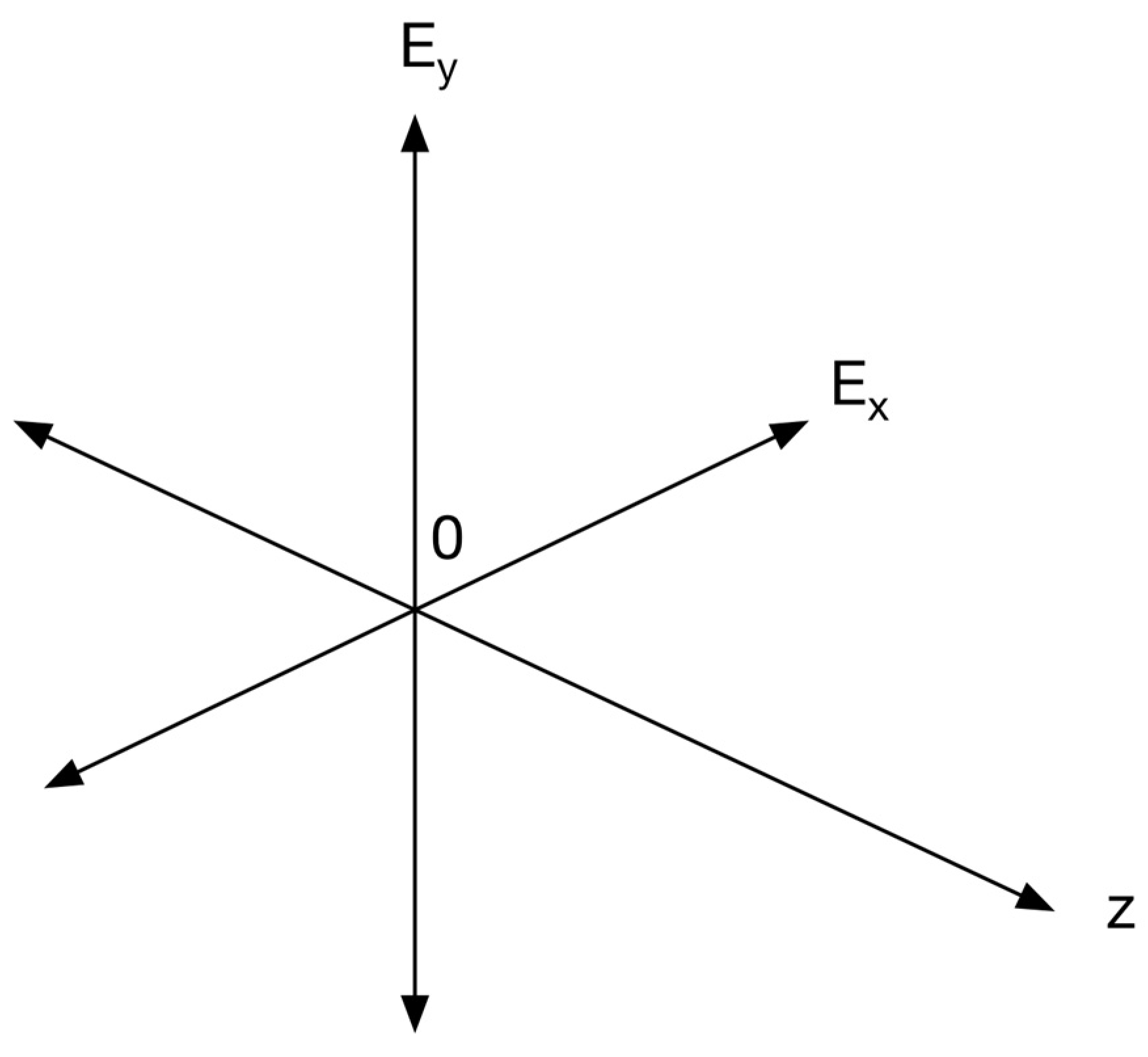
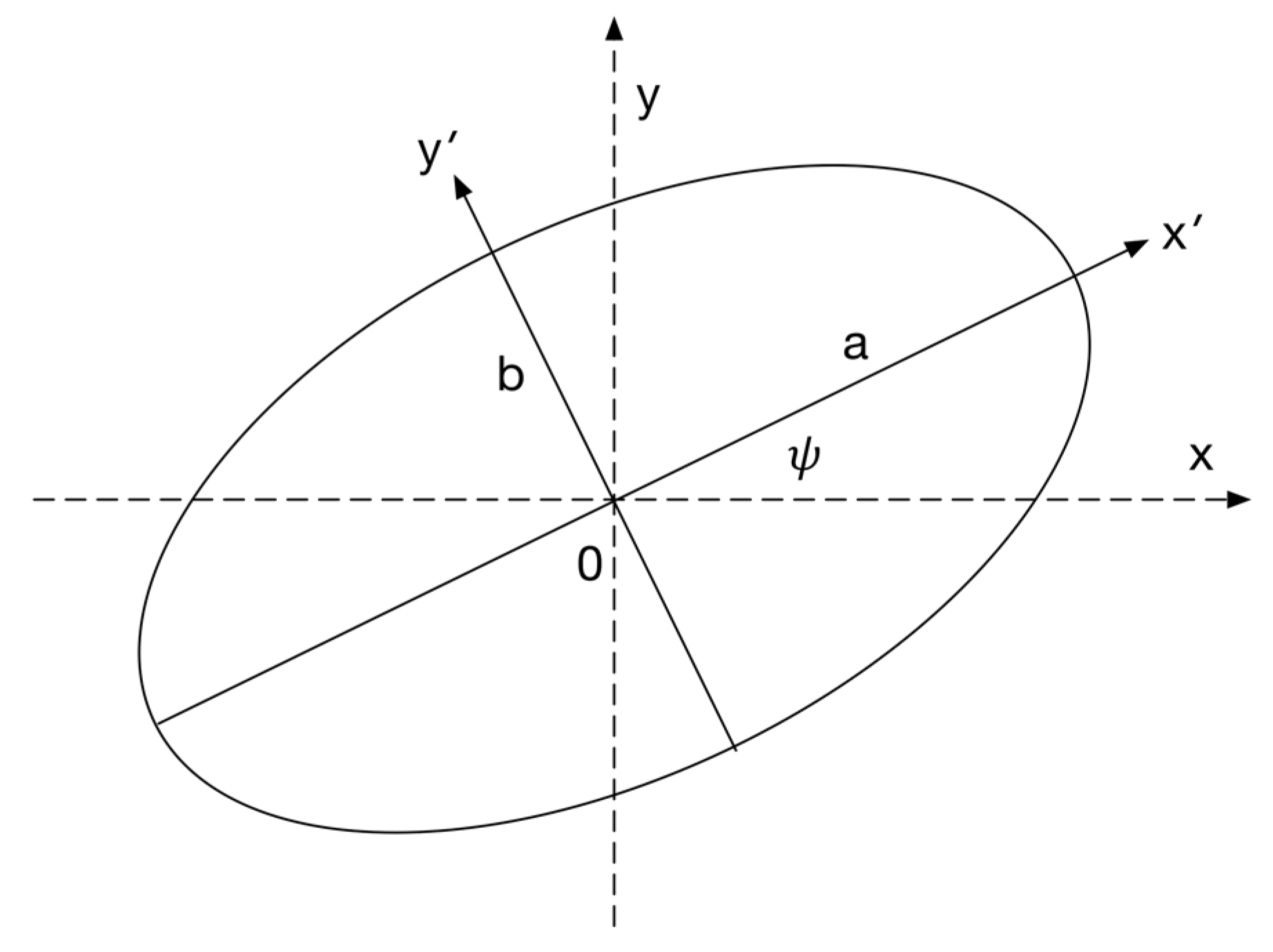
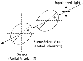
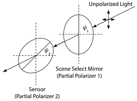
2.1. The Polarization Ellipse
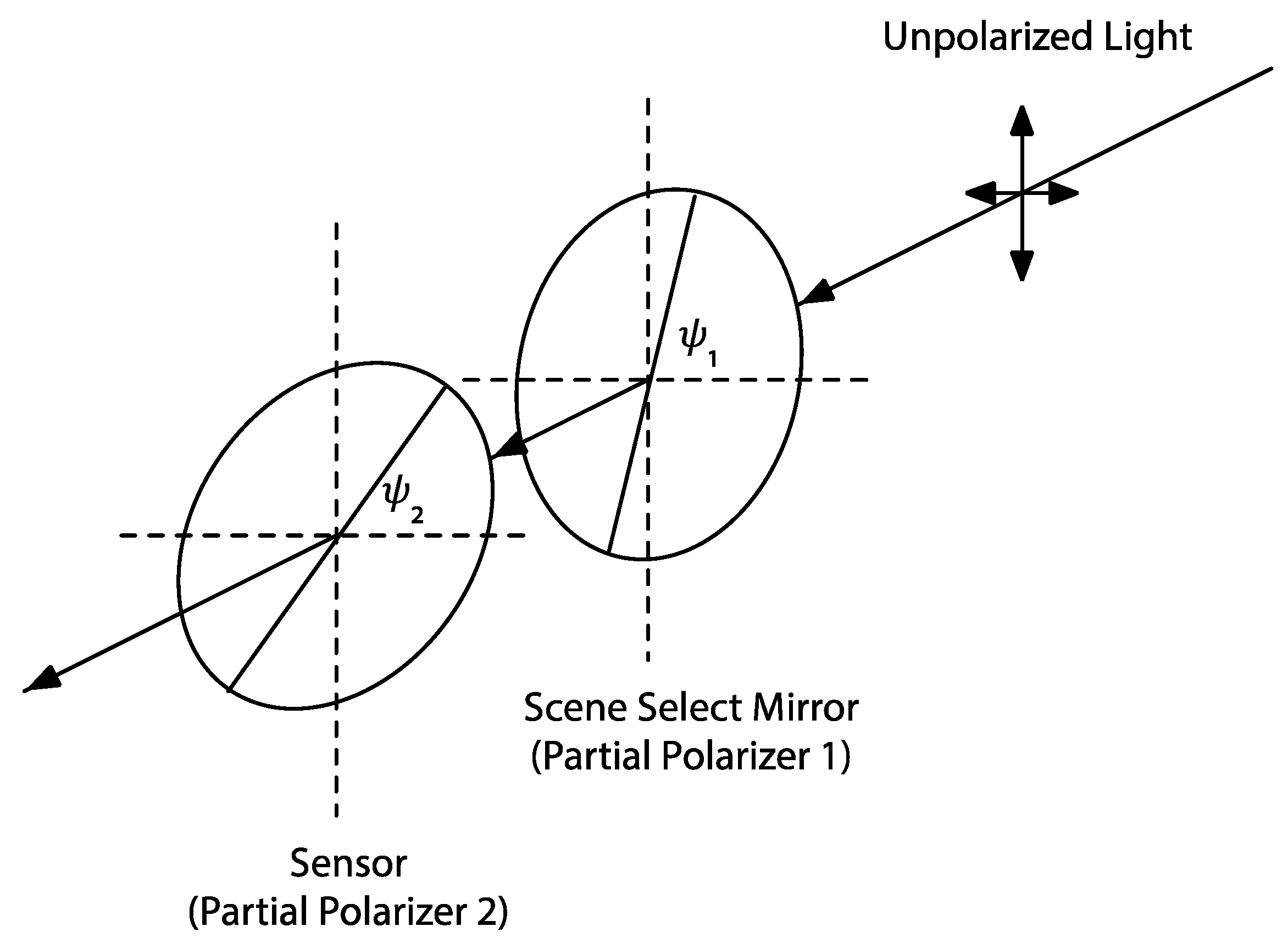
2.2. Calibration Bias due to Polarization
3. Polarization-Induced Calibration Biases
3.1. Polarization-Induced Calibration Bias Theoretical Model
3.2. Modeling CrIS Polarization-Induced Calibration Error
4. The CrIS Polarization Parameters
4.1. Pitch Maneuver Overview
4.2. Pitch Maneuver Dataset Description
4.3. Pitch Maneuver Analysis and Results
5. Correction of Earth Scene Radiances for Radiometric Modulation due to Polarization
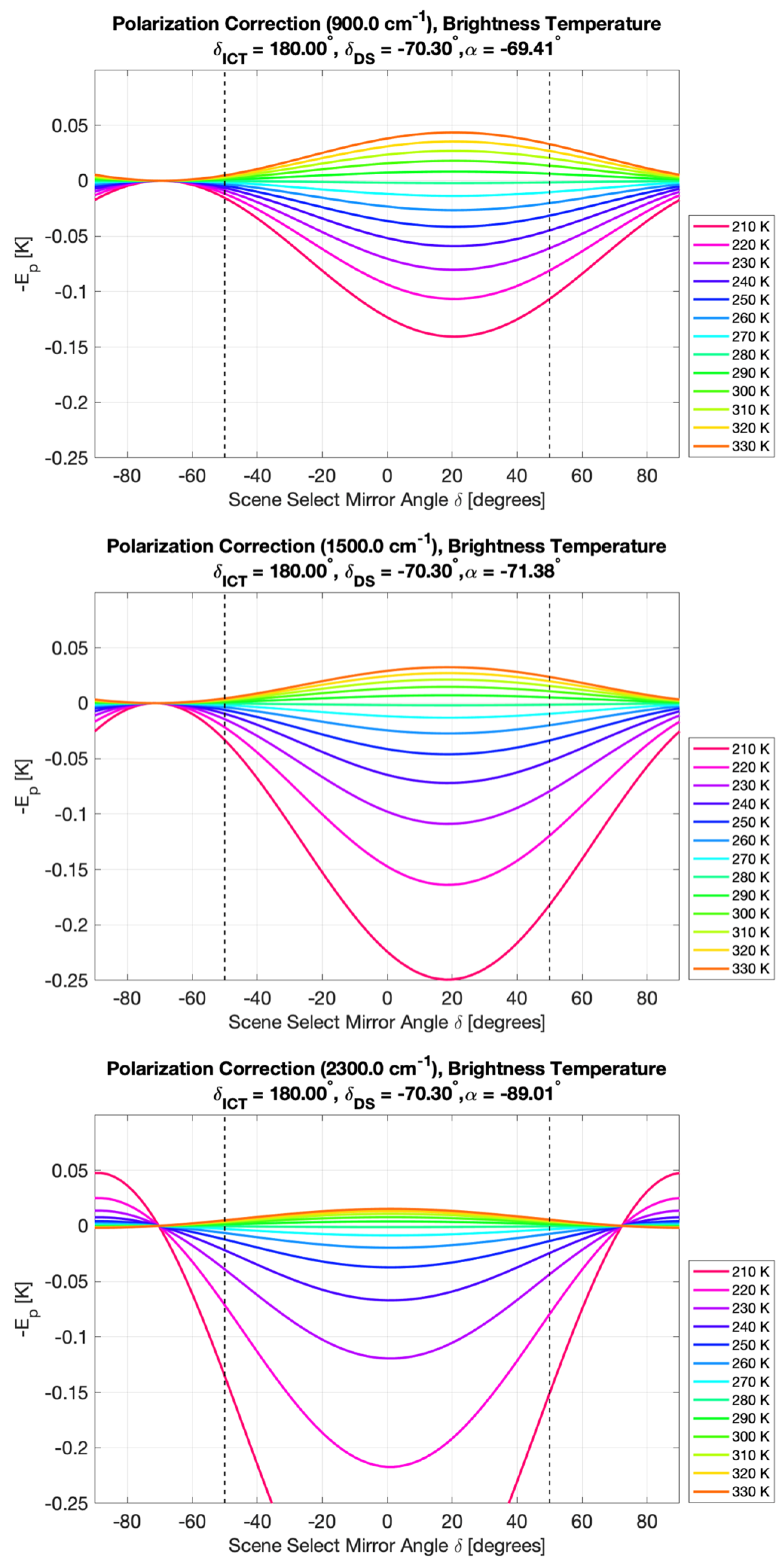
5.1. FOR and Scene Temperature Dependence of the Polarization Correction
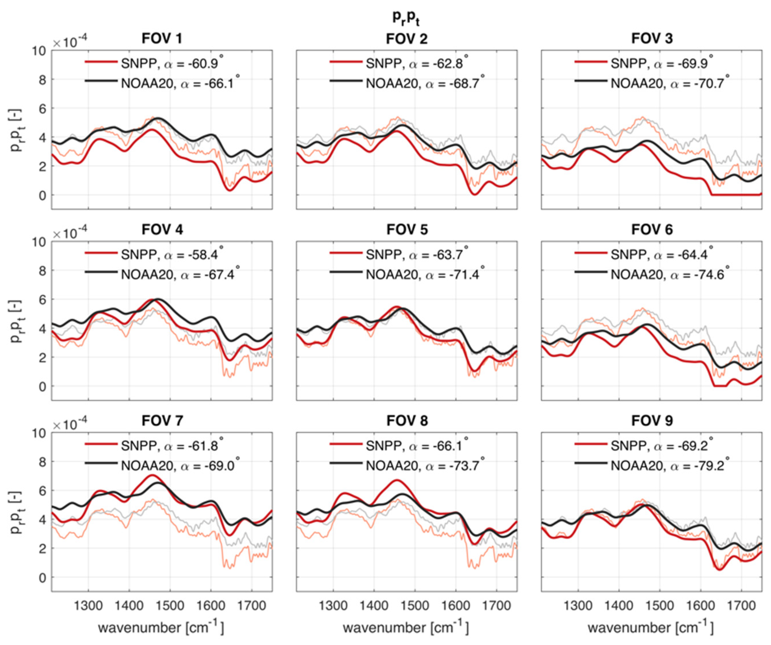
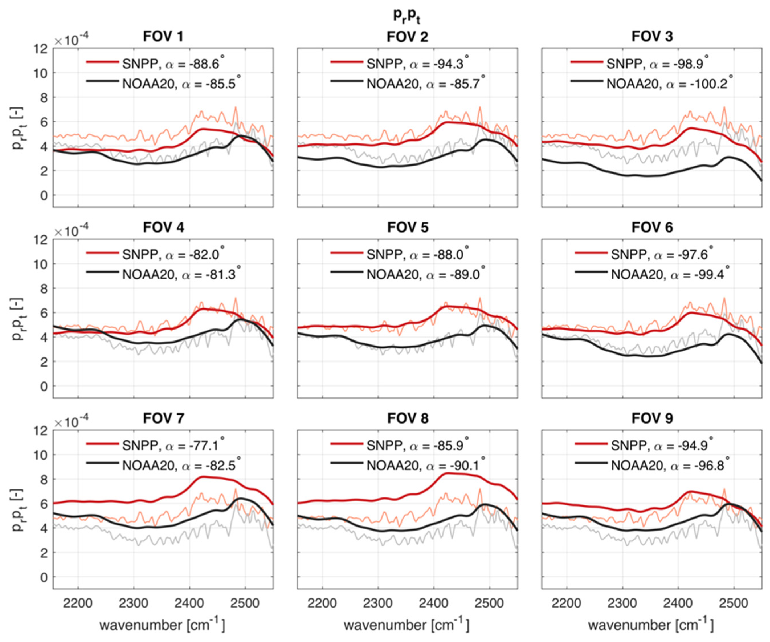
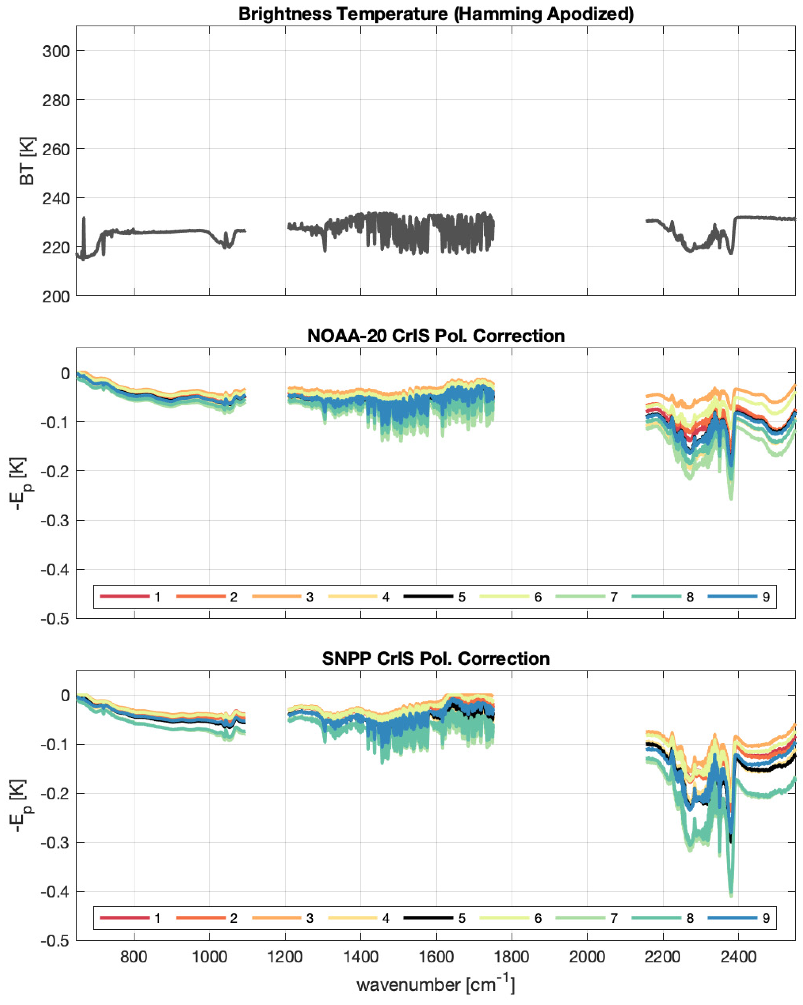
5.2. FOV and Sensor Dependence of the Polarization Correction
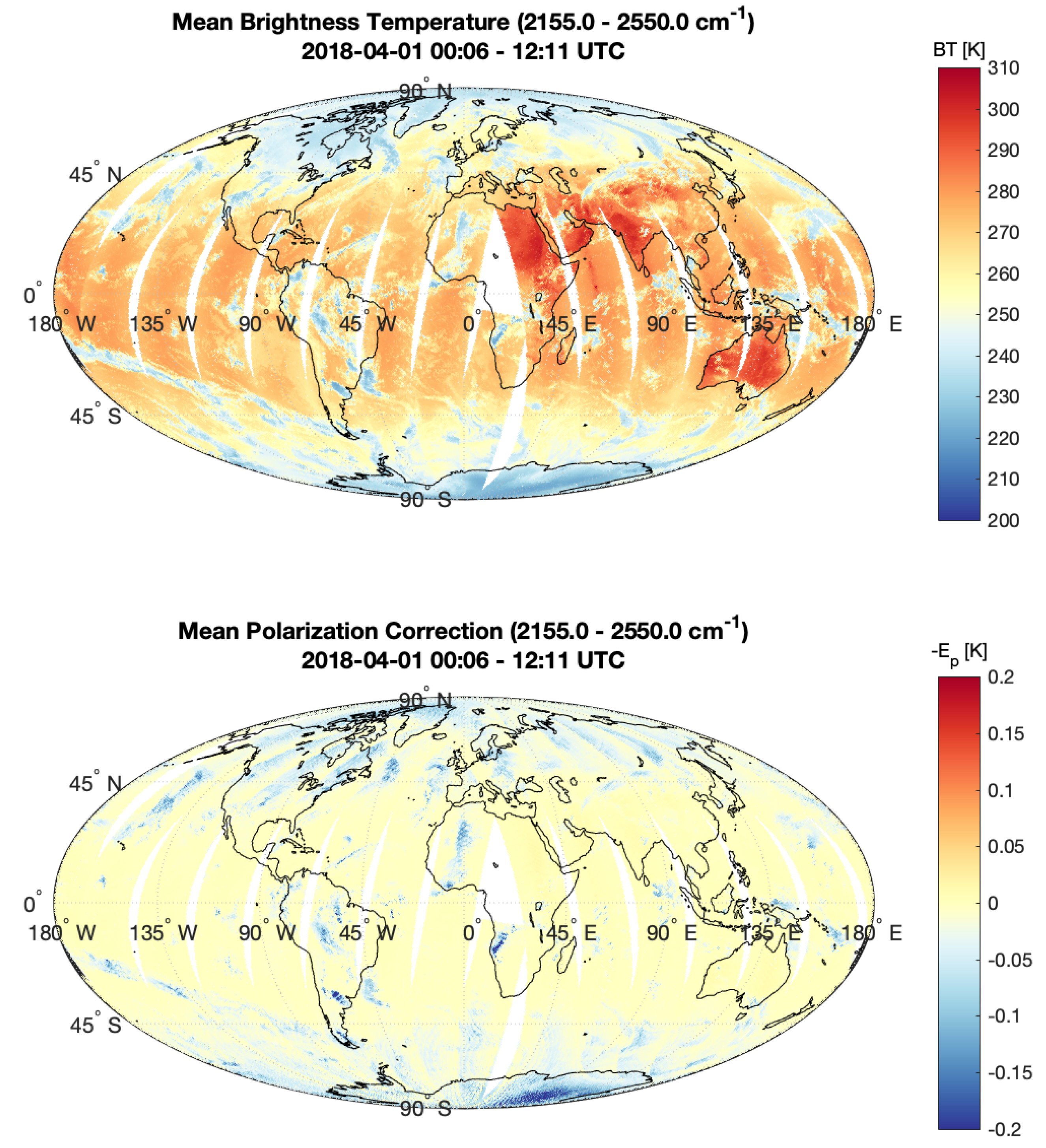
5.3. Polarization Correction Results: Global Coverage
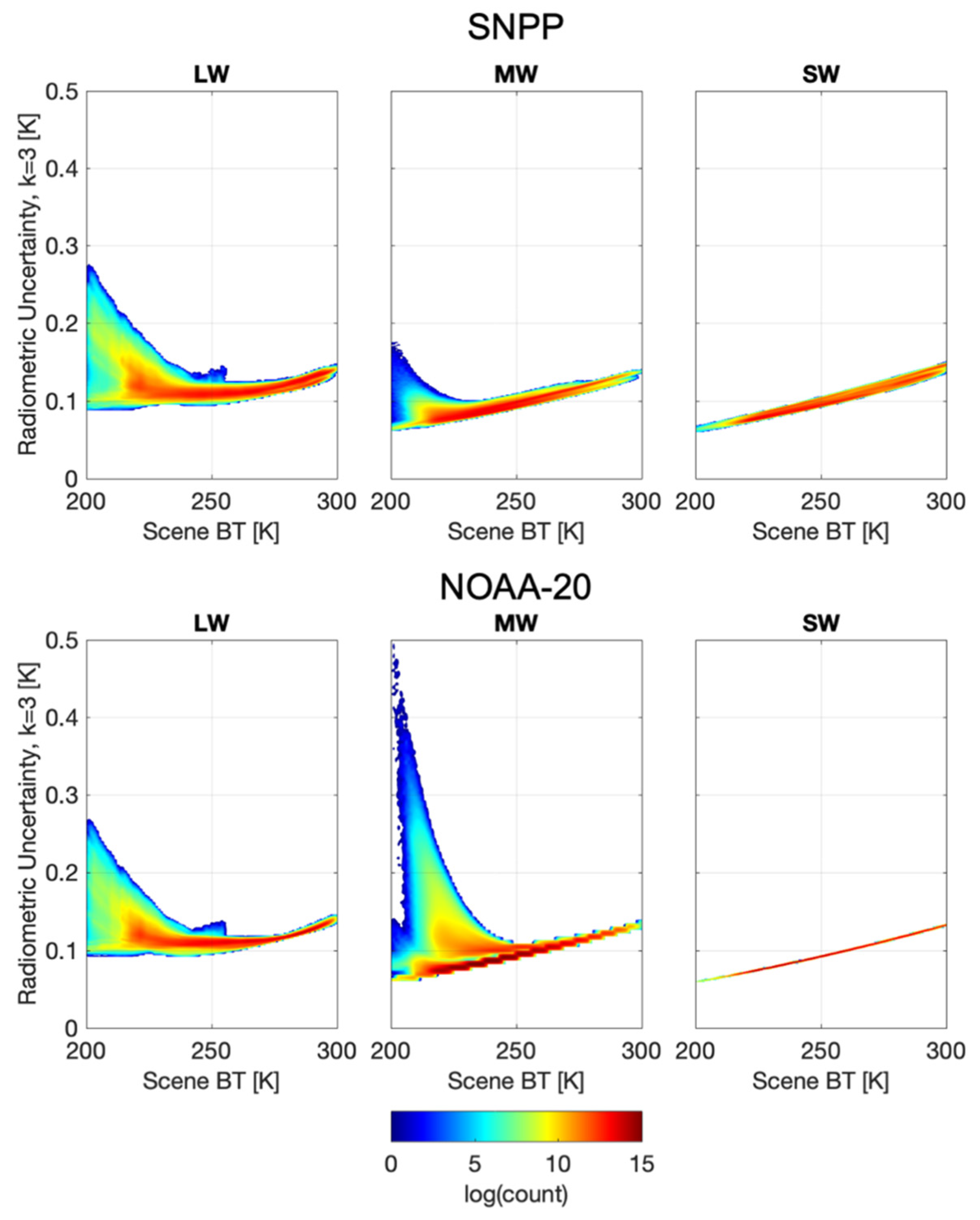
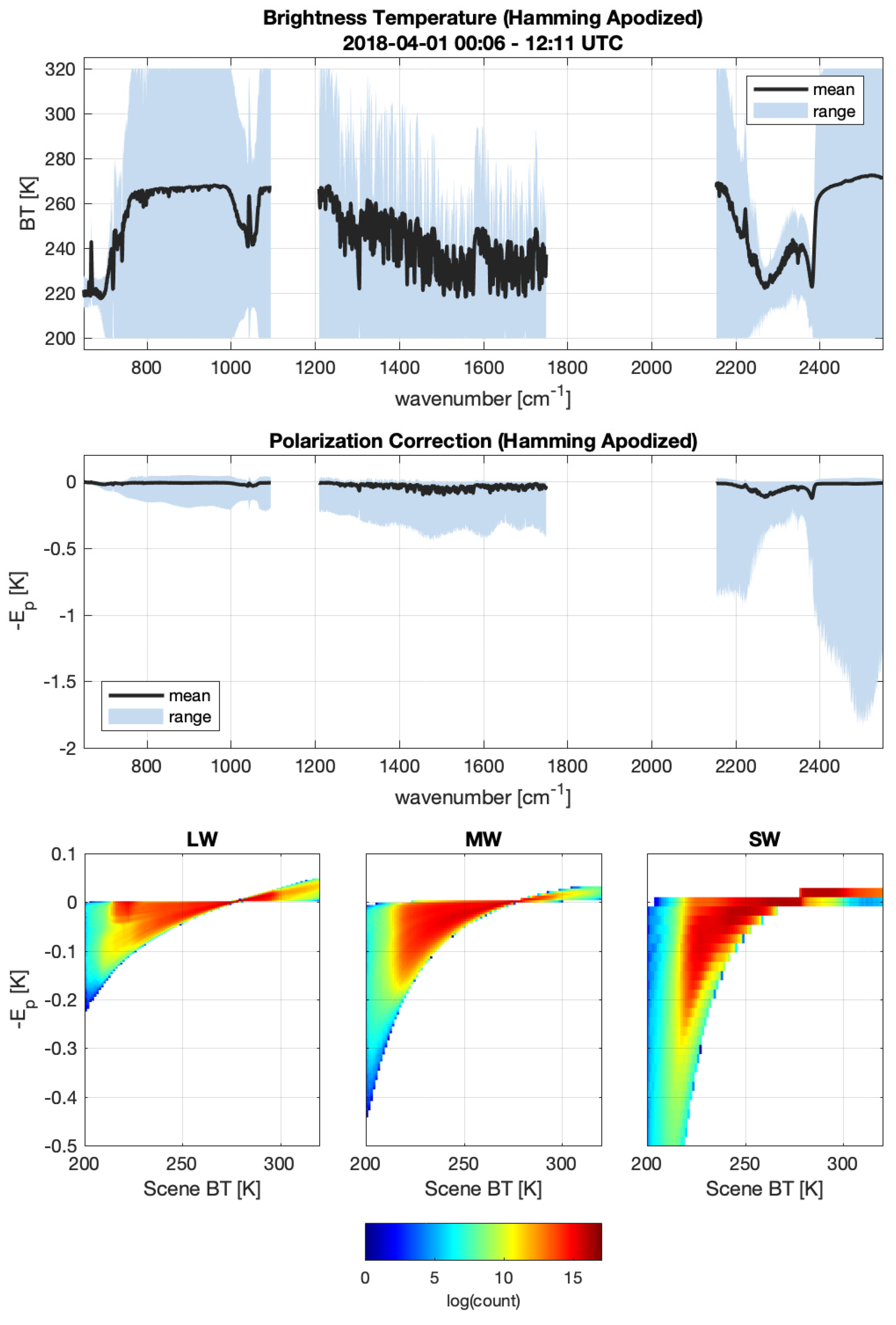
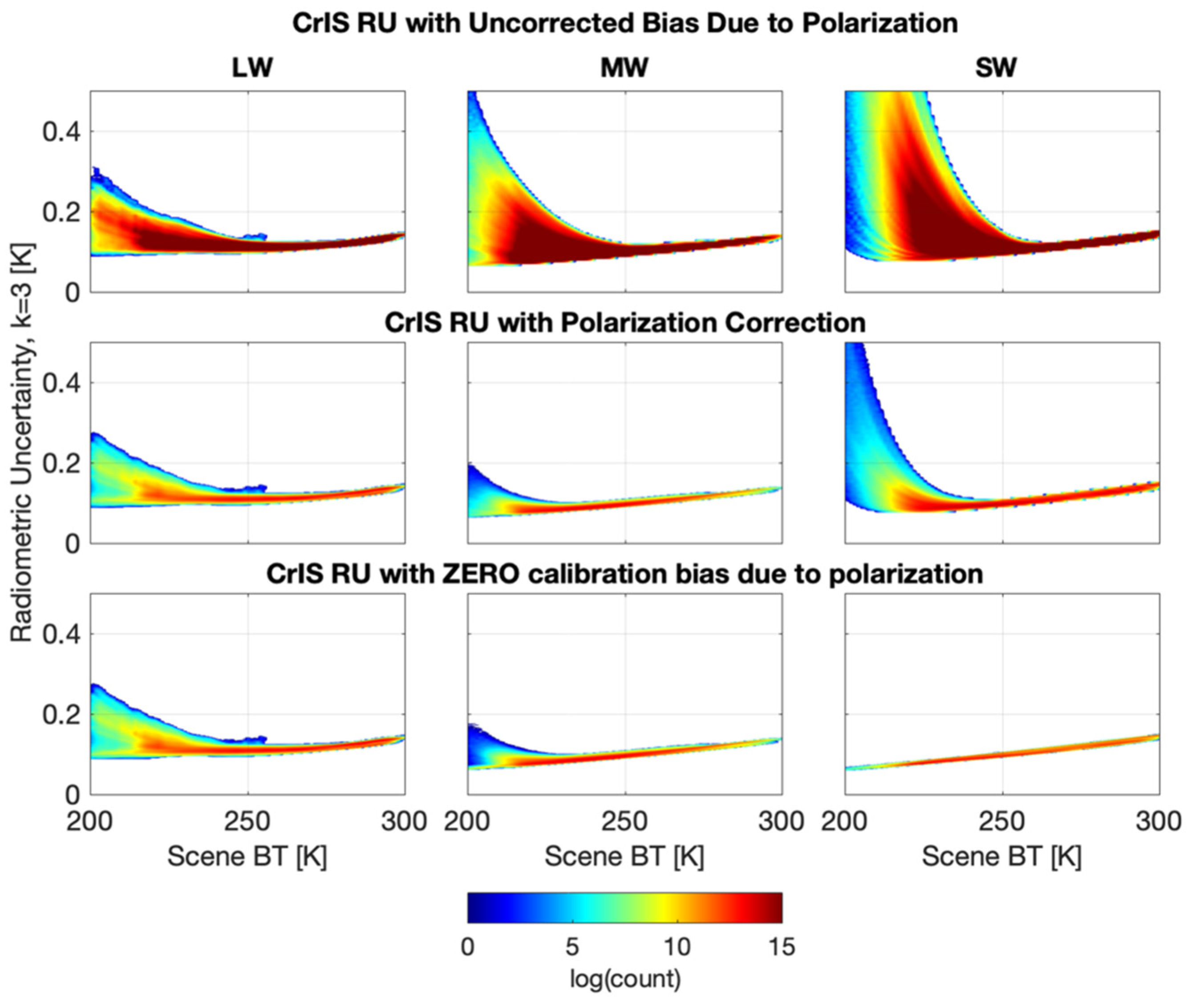
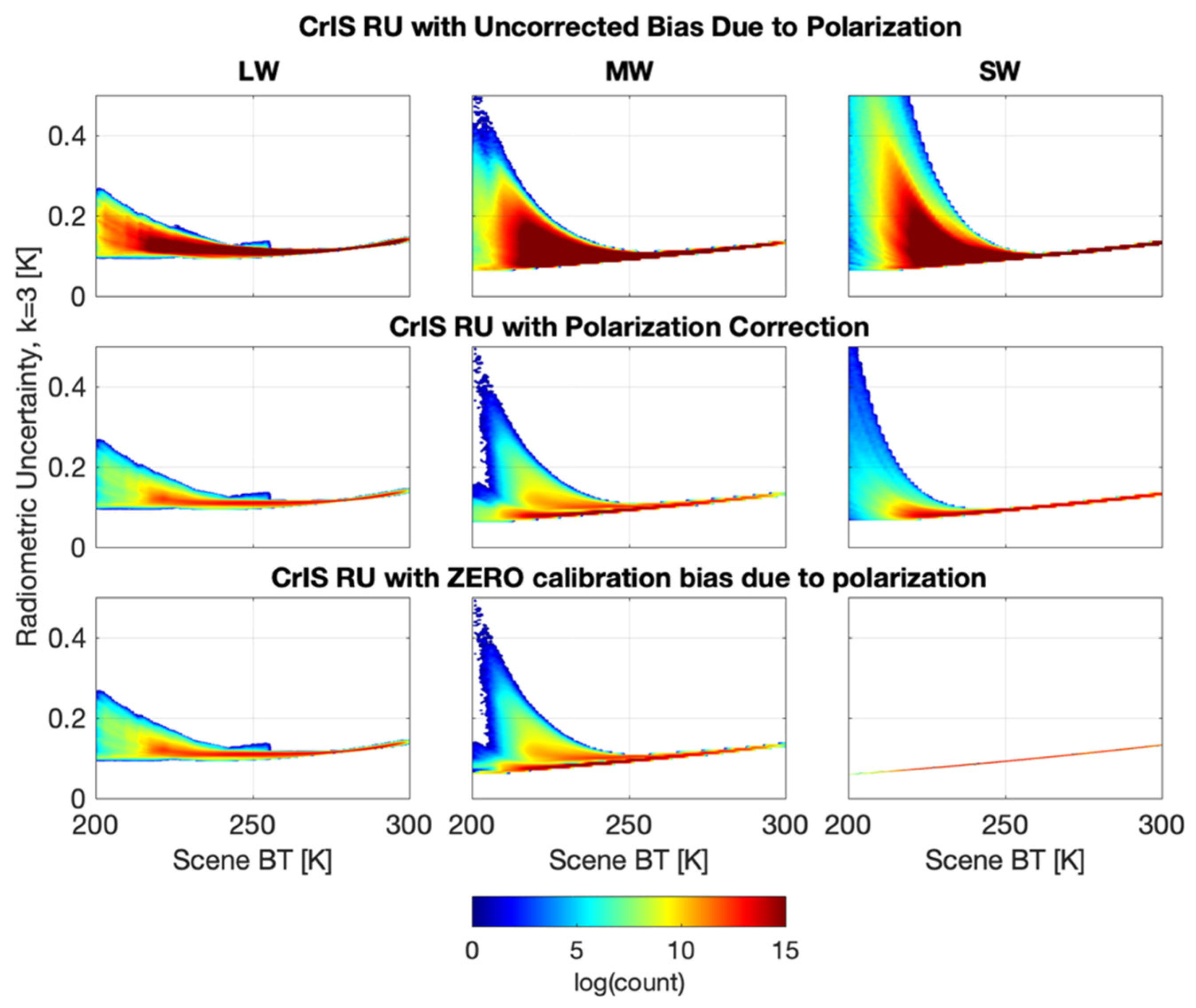
5.4. Estimated Radiometric Uncertainty Associated with Correction
- The Internal Calibration Target (ICT) temperature, ICT effective cavity emissivity, and the temperatures of the reflected terms in the ICT environmental model,
- The quadratic coefficient in the nonlinearity correction,
- The polarization correction parameters (combined scene mirror and sensor polarization and the sensor polarization angle).
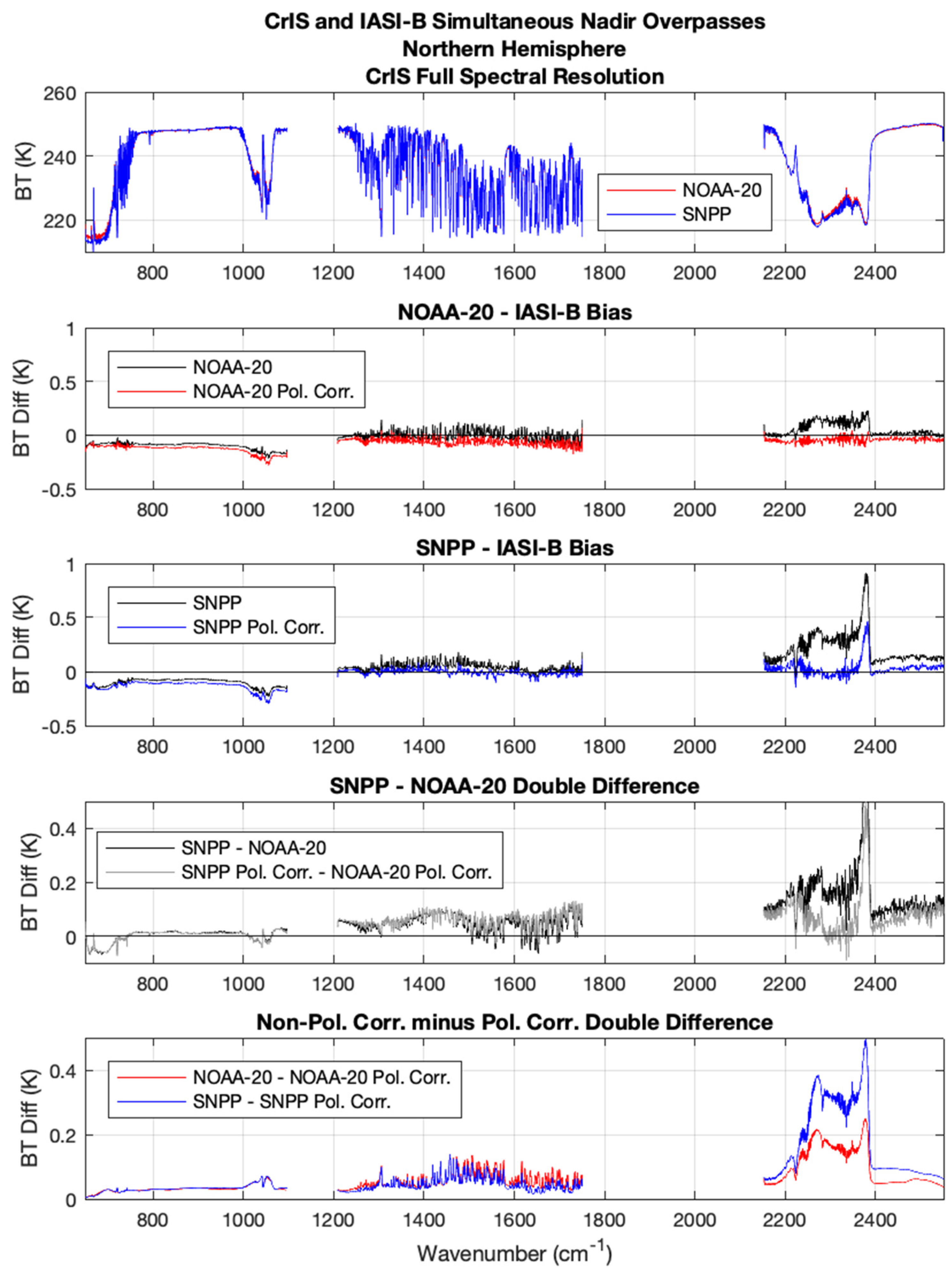
6. Impact on Inter-Instrument Comparisons
7. Summary
Author Contributions
Funding
Data Availability Statement
Acknowledgments
Conflicts of Interest
References
- Eresmaa, R.; Letertre-Danczak, J.; Lupu, C.; Bormann, N.; McNally, A.P. The assimilation of Cross-track Infrared Sounder radiances at ECMWF. Q. J. R. Meteorol. Soc. 2017, 143, 3177–3188. [Google Scholar] [CrossRef]
- Knight, E.; Merrow, C.; Salo, C. Interaction between Polarization and Response vs. Scan Angle in the Calibration of Imaging Radiometers; SPIE: Bellingham, WA, USA, 1999; Volume 3754. [Google Scholar]
- Pagano, T.; Aumann, H.; Overoye, K.; Gigioli, G. Scan-Angle-Dependent Radiometric Modulation Due to Polarization for the Atmospheric Infrared Sounder (AIRS); SPIE: Bellingham, WA, USA, 2000; Volume 4135. [Google Scholar]
- Shaw, J.A. The effect of instrument polarization sensitivity on sea surface remote sensing with infrared spectroradiometers. J. Atmos. Ocean. Technol. 2002, 19, 820–827. [Google Scholar]
- Sun, J.Q.; Xiong, X. MODIS polarization-sensitivity analysis. Geosci. Remote Sens. IEEE Trans. 2007, 45, 2875–2885. [Google Scholar]
- Young, J.; Knight, E.; Merrow, C. MODIS Polarization Performance and Anomalous Four-Cycle Polarization Phenomenon; SPIE: Bellingham, WA, USA, 1998; Volume 3439. [Google Scholar]
- Tobin, D.; Revercomb, H.; Knuteson, R.; Taylor, J.; Best, F.; Borg, L.; DeSlover, D.; Martin, G.; Buijs, H.; Esplin, M.; et al. Suomi-NPP CrIS radiometric calibration uncertainty. J. Geophys. Res. Atmos. 2013, 118, 10589–510600. [Google Scholar] [CrossRef]
- Hecht, E. Optics, 4th ed.; Addison Wesley: Boston, MA, USA, 2002. [Google Scholar]
- Collett, E. Field Guide to Polarization; SPIE Press: Bellingham, WA, USA, 2005; Volume 15. [Google Scholar]
- Goldstein, D. Polarized Light; Marcel Dekker: New York, NY, USA, 2003; Volume 2003, p. 1. [Google Scholar]
- Revercomb, H.E. Polarization Effects: Theory and Characterization for Correction; Space Science and Engineering Center, University of Wisconsin–Madison: Madison, WI, USA, 2013; pp. 1–3. [Google Scholar]
- Taylor, J.K. Achieving 0.1 K Absolute Calibration Accuracy for High Spectral Resolution Infrared and Far Infrared Climate Benchmark Measurements; Université Laval: Québec, QC, Canada, 2014. [Google Scholar]
- Aumann, H.; Gaiser, S.; Ting, D.; Manning, E. AIRS Algorithm Theoretical Basis Document Level 1B Part 1: Infrared Spectrometer; OS Project Science Office, NASA Goddard Space Flight Center: Greenbelt, MD, USA, 1999. [Google Scholar]
- Revercomb, H.E.; Buijs, H.; Howell, H.B.; LaPorte, D.D.; Smith, W.L.; Sromovsky, L.A. Radiometric calibration of IR Fourier transform spectrometers: Solution to a problem with the High-Resolution Interferometer Sounder. Appl. Opt. 1988, 27, 3210–3218. [Google Scholar] [PubMed]
- Iturbide-Sanchez, F. Joint Polar Satellite System (JPSS) Cross Track Infrared Sounder (CrIS) Sensor Data Records (SDR) Algorithm Theoretical Basis Document (ATBD) for Full Spectral Resolution; JPSS Configuration Management Office: Greenbelt, MD, USA, 2018. [Google Scholar]
- Taylor, J.; Revercomb, H.; Best, F.; Gero, P.J.; Genest, J.; Buijs, H.; Grandmont, F.; Tobin, D.; Knuteson, R. The University of Wisconsin Space Science and Engineering Center Absolute Radiance Interferometer (ARI): Instrument Overview and Radiometric Performance; SPIE: Bellingham, WA, USA, 2014; Volume 9263. [Google Scholar]
- Taylor, J.K.; Revercomb, H.E.; Best, F.A.; Tobin, D.C.; Gero, P.J. The Infrared Absolute Radiance Interferometer (ARI) for CLARREO. Remote Sens. 2020, 12, 1915. [Google Scholar] [CrossRef]
- Butler, J.J.; Xiong, X.; Barnes, R.A.; Patt, F.S.; Sun, J.; Chiang, K. An overview of Suomi NPP VIIRS calibration maneuvers. In Earth Observing Systems XVII; SPIE: Bellingham, WA, USA, 2012; p. 85101. [Google Scholar]


| Illustration | Relative Orientation of SSM and Sensor Polarization | Transmission of Unpolarized Light |
|---|---|---|
 | ||
 | ||
 |
| Description | Value | Notes | |
|---|---|---|---|
| Temperatures | |||
| Cold Cal Ref, Deep Space View (DS) | 2.8 K | Effective brightness temperature of the DS view | |
| Hot Cal Ref, Internal Calibration Target (ICT) | 282 K | Should represent typical on-orbit temperature | |
| Earth Scene or External Target Temperature | 210–330 K | ||
| SSM Temperature | 282 K | Average instrument background temperature | |
| Reflected Radiance, Cold Cal Ref | 282 K | ||
| Reflected Radiance, Hot Cal Ref | 282 K | ||
| Reflected Radiance, Scene or Ext. Target | 282 K | ||
| Emissivities | |||
| Cold Cal Ref, Deep Space View, (DS) | 1 | A perfect DS view will have an effective emissivity of unity | |
| Hot Cal Ref, Internal Cal Target (ICT) | 1 | Set to unity for initial model | |
| Earth Scene | 1 | Set to unity for initial model | |
| Polarization | |||
| Instrument polarization ellipse, angle | 0° | The model depends on , not the absolute angular position of either or . Hence, the choice of the 0° position is arbitrary, and the angular position of the nadir view was chosen as the 0° reference for convenience. | |
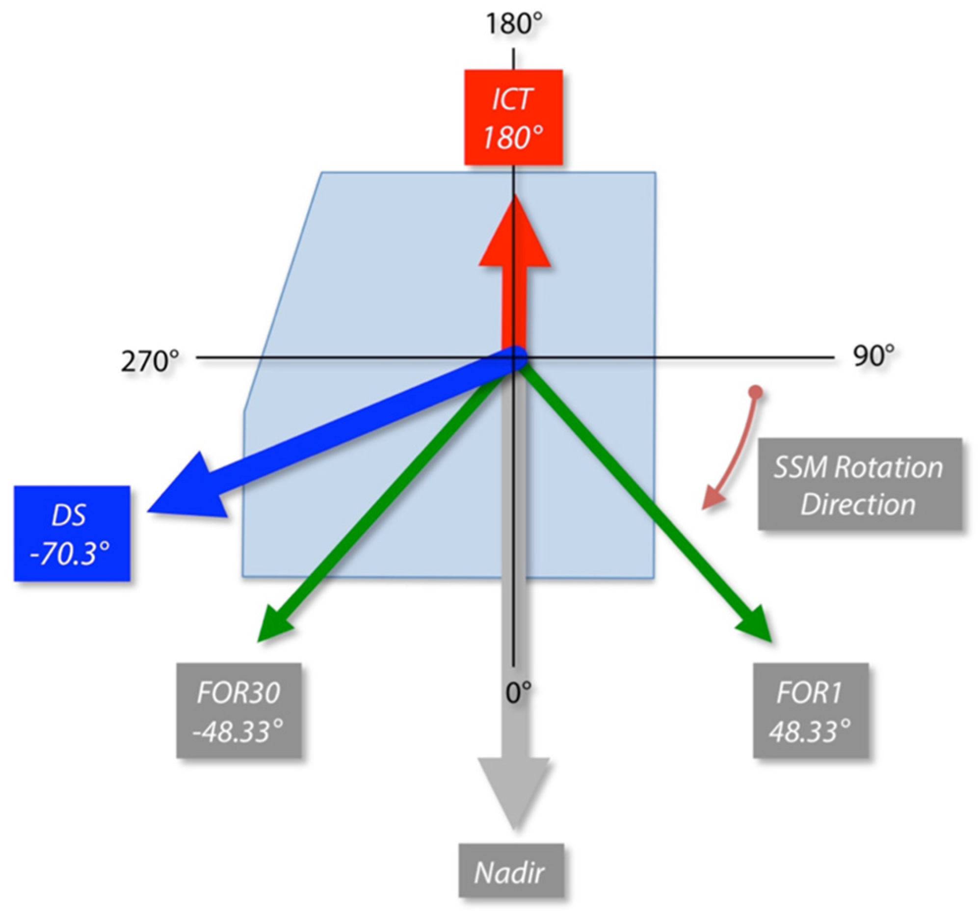
| Cold Cal Ref (DS) Position (Nominal) | −70.3° | ||
| Hot Cal Ref (ICT) Position (Nominal) | 180° | ||
| Cross-track FOR Angles (Nominal) | −48.33° to 48.33° | ||
Disclaimer/Publisher’s Note: The statements, opinions and data contained in all publications are solely those of the individual author(s) and contributor(s) and not of MDPI and/or the editor(s). MDPI and/or the editor(s) disclaim responsibility for any injury to people or property resulting from any ideas, methods, instructions or products referred to in the content. |
© 2023 by the authors. Licensee MDPI, Basel, Switzerland. This article is an open access article distributed under the terms and conditions of the Creative Commons Attribution (CC BY) license (https://creativecommons.org/licenses/by/4.0/).
Share and Cite
Taylor, J.K.; Revercomb, H.E.; Tobin, D.C.; Knuteson, R.O.; Loveless, M.L.; Malloy, R.; Suwinski, L.; Iturbide-Sanchez, F.; Chen, Y.; White, G.; et al. Assessment and Correction of View Angle Dependent Radiometric Modulation due to Polarization for the Cross-Track Infrared Sounder (CrIS). Remote Sens. 2023, 15, 718. https://doi.org/10.3390/rs15030718
Taylor JK, Revercomb HE, Tobin DC, Knuteson RO, Loveless ML, Malloy R, Suwinski L, Iturbide-Sanchez F, Chen Y, White G, et al. Assessment and Correction of View Angle Dependent Radiometric Modulation due to Polarization for the Cross-Track Infrared Sounder (CrIS). Remote Sensing. 2023; 15(3):718. https://doi.org/10.3390/rs15030718
Chicago/Turabian StyleTaylor, Joe K., Henry E. Revercomb, David C. Tobin, Robert O. Knuteson, Michelle L. Loveless, Rebecca Malloy, Lawrence Suwinski, Flavio Iturbide-Sanchez, Yong Chen, Glen White, and et al. 2023. "Assessment and Correction of View Angle Dependent Radiometric Modulation due to Polarization for the Cross-Track Infrared Sounder (CrIS)" Remote Sensing 15, no. 3: 718. https://doi.org/10.3390/rs15030718
APA StyleTaylor, J. K., Revercomb, H. E., Tobin, D. C., Knuteson, R. O., Loveless, M. L., Malloy, R., Suwinski, L., Iturbide-Sanchez, F., Chen, Y., White, G., Predina, J., & Johnson, D. G. (2023). Assessment and Correction of View Angle Dependent Radiometric Modulation due to Polarization for the Cross-Track Infrared Sounder (CrIS). Remote Sensing, 15(3), 718. https://doi.org/10.3390/rs15030718