Abstract
Atmospheric correction is the processes of converting radiance values measured at a spectral sensor to the reflectance values of the materials in a multispectral or hyperspectral image. This is an important step for detecting or identifying the materials present in the pixel spectra. We present two machine learning models for atmospheric correction trained and tested on 100,000 batches of 40 reflectance spectra converted to radiance using MODTRAN, so the machine learning model learns the radiative transfer physics from MODTRAN. We created a theoretically interpretable Bayesian Gaussian process model and a deep learning autoencoder treating the atmosphere as noise. We compare both methods for estimating gain in the correction model to process for estimating gain within the well-know QUAC method which assumes a constant mean endmember reflectance. Prediction of reflectance using the Gaussian process model outperforms the other methods in terms of both accuracy and reliability.
1. Introduction
Atmospheric correction of a hyperspectral or multispectral image is the process of converting the observed at-sensor radiance (the amount of light per wavelength measured at the sensor) to ground reflectance (the percent reflectance per wavelength of the material(s) located at on the ground). This is an essential step when using hyperspectral imagery to identify the materials in pixels, so that the pixel spectra provide information about the materials and not the illumination and atmospheric variation.
In this paper we present two methods for machine learning of atmospheric radiative transfer from collections of spectra from a hyperspectral image. Each method takes in a collection observed pixel spectra from a hyperspectral image and outputs the reflectance spectra for the pixels, providing coefficients for atmospheric correction that can be applied to the entire image.
1.1. Background
A hyperspectral image is a digital image in which each pixel has more than the visual three color (red, green, blue) bands, but often hundreds of bands across wavelengths sufficient to get spectral information about the materials in each pixel. We focus on hyperspectral images that have band wavelengths from about 400 nm to 2500 nm—for comparison the visual colors occur around 450 nm (blue), 550 nm (green) and 650 nm (red)—and our spectra have 452 bands as collected with 375 bands after removing bands where the signal is absorbed by atmospheric water vapor. For a hyperspectral image collected at these wavelengths, the measured light at the sensor is primarily reflected sunlight, having passed through the atmosphere, reflected off materials, and passed again through some amount of atmosphere (which may be small for a ground-based space or significant if the sensor is on board an aircraft or satellite.) Each band is typically 2 nm to 10 nm wide, and the bands are contiguous across the wavelength range. The reflectance for a material is important because it is the result of the interaction of photons at different wavelengths and the resonant frequencies of molecular bonds (for the wavelengths above the visible range) and the interaction of photons and electrons moving between quantum states (for wavelengths around the visible range). Specifically, important information about the constituents and bonds present in a material can be computed from reflectance spectra, for example distinguishing between different polymers, or distinguishing talcum powder from powdered sugar from dangerous white powdered substances.
As light propagates through the atmosphere, some light is absorbed by the particles and gases in the atmosphere, some light is scattered, and some light passes through the atmosphere. Light at lower wavelengths has greater probability of being scattered (the blue sky effect), and generally the fraction of light that is absorbed varies with wavelength, depending on the gasses and particles present. The percentage of light that passes through the atmosphere is called transmittance, which is a function of wavelength for a given atmosphere. This transmittance can be computed from physical measurements for a given atmosphere (density of water vapor, sun and sensor angles, etc.) using MODTRAN [1] (MODerate resolution atmospheric TRANsmission) software. A plot of transmittance for two different atmospheric models created using the MODTRAN online interface (http://modtran.spectral.com/modtran_home, accessed on 23 December 2022) across our wavelength range with a spectral resolution (band width) of 5 nm is shown in Figure 1. Observe that these two spectra differ in magnitude and in depth of the absorption features that occur at various wavelengths. The transmittance labeled US Std 1976 was created using the US Standard 1976 Atmospheric model, water column of 1162.3 atm-cm, ozone column of 0.3456 atm-cm, of 400 ppmv, of 0.15 ppmv, of 1.8 ppmv, ground temperature of 288.15 K, a Rural Aerosol model, 13 km visibility, sensor altitude of 50 km, and sensor zenith angle of 180 deg. The transmittance labeled Mid-Lat Summer was created using the Mid-Latitude Summer model with a water column of 3635.9 atm-cm, ozone column of 0.33176 atm-cm, ground temperature of 294.2 K, and solar zenith of 135 deg, and all other parameters equal to those for the US Std 1976 transmittance. Our main goal includes determining this transmittance fraction from spectra on the ground measured from a sensor even when the reflectance of the ground material is unknown.
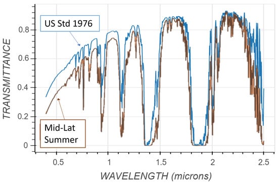
Figure 1.
Two plots of transmittance for two different atmospheric models created using the MODTRAN online interface.
The plot in Figure 2 shows more components involved in the radiative transfer model. The plots (left) were generated with the MODTRAN online interface. The Direct Solar (100 km) gives the amount of sunlight measured at the top of the atmosphere. The main shape of this curve is from the blackbody radiation given the temperature of the sun. The Direct Solar (0 km) is the amount of sunlight reaching the ground, which is the Direct Solar (100 km) times a transmittance similar to that shown in Figure 1. The Downward Diffuse (0 km) is the amount of light per wavelength that reaches the ground after scattering in the atmosphere; this is the indirect illumination on an object, for example on an object in a shadow from the sun. The upward Diffuse is the amount of upward light, which at 100 km (top of atmosphere) is from atmospheric scattering and at 0 km is from the blackbody radiation of the ground (which is insignificant given the wavelength range and ground temperature assumed in this model).
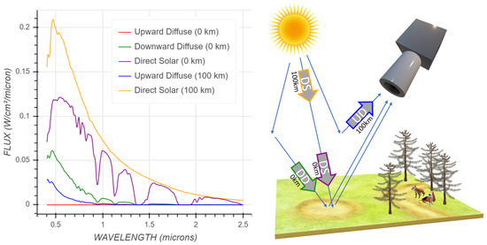
Figure 2.
Components of the atmospheric radiative transfer model created using the MODTRAN online interface (left). The at-sensor radiance is the sum of all light entering the sensor, which is the result of these components and their interaction with the ground (right). The components shown in the left-hand figure were created using a Mid-Latitude Summer atmosphere model and a Rural aerosol model, with all parameters at default values for these models. The parameters correspond to the labeled paths on the right-hand figure: UD = Upward Diffuse, etc.
The at-sensor radiance is the Upward Diffuse (at the elevation of the sensor) plus the total illumination at the ground (Direct Solar + Downward Diffuse) times the percent reflectance per band of the material on the ground per wavelength . Using the abbreviations for these components as shown in Figure 2, this is
There are additional nonlinear effects as well which are not shown in Figure 2. Light that has passed through a leaf and reflected off the ground would have the leaf transmittance times ground reflectance in place of in this equation. In the lower wavelengths, especially blue and below, photons will take multiple bounces/scattering (collectively, ’haze’ in the image) in the atmosphere. This multiple bounce haze causes additional upward diffuse and additional downward diffuse illumination on the ground. There are also photons that reflect off material at one ground location and then scatter in the atmosphere to enter the sensor at locations/directions for other pixels, causing an “Upward Diffuse” that varies across the image comprised of a nonlinear mixture of nearby ground material spectra and atmospherics, rather than the ideal Upward Diffuse from the atmosphere alone shown in Figure 2. These nonlinear effects are minimal in most cases.
All of these values change with respect to atmospheric constituents, water vapor, CO2, Ozone, CH4, aerosols, sun angle, fraction of sun and sky visible to each pixel (shadow from objects, terrain, clouds, etc.), sensor angle, angle and roughness of the ground material, and other factors. The MODTRAN software can simulate these effects if they are known, and provide a modeled at-sensor radiance for reflectance spectra, or an approximated ground reflectance spectrum for a measured at sensor radiance.
1.2. Significance
The purpose of hyperspectral imaging is to perform spectroscopy writ large; that is, to be able to determine the materials in each pixel from the reflectance spectra for those pixels. As such, good atmospheric compensation is an essential step. Before atmospheric compensation is applied, the spectral are primarily the result of atmospheric absorption. After applying atmospheric compensation, the spectra in the image are the actual spectra of the materials on the ground. Without this step, it is impossible to compare image pixel spectra to laboratory measurements of known materials.
1.3. Related Works
The most accurate methods either use physics-based modelling with MODTRAN such as FLAASH [2] or using materials of known reflectance in the image, for example the empirical line method [3,4], in which case it is usually preferable to have materials that are spectrally flat, for example a set of five panels which are 5%, 30% 50% 80% and 95% reflectance across all wavelengths, which can be used to estimate a best fit regression line per wavelength to convert from radiance units to reflectance. However, both of these methods make approximations in their modelling of physical parameters. For example, a good ELM will estimate the upward diffuse as the intercept and the direct solar and downward diffuse as the slope, but assume these are consistent values for every pixel in the image. FLAASH attempts to estimate the physical parameters from the image radiance spectra based on user input of parameters, even estimating water vapor content per pixel, and use a physics based model to compute the grouped reflectance from each at-sensor radiance measurement.
A heuristic and approximate but surprisingly effective method for atmospheric compensation is to make the assumption that the mean spectrum of a significantly large diverse library of reflectance spectra will be constant (independent of the spectra used and varying only with wavelength, called the ideal mean reflectance), and use this assumption to compute a single gain and offset that is applied per wavelength across the image. A method based on this assumption is QUAC [5] (QUick Atmospheric Correction), which functions approximately as follows. First, the minimum measured radiance value across the image per wavelength is assumed to be the upwelling radiance at the sensor (offset), and is thus subtracted from the image. The top of atmosphere solar radiance (Direct Solar in Figure 2) is approximated using a plank function at the observed temperature of the sun, and this value is divided by the radiance values per band as a first step in correcting for illumination intensity. Then a sample of 50 different spectra (called endmembers) are selected from the radiance image, usually iteratively so each new endmember is optimally different than the previous ones, and the mean of these 50 endmembers is determined. Then the ratio between the ideal mean and mean of the endmembers is computed and used as a ’gain’ and is multiplied by every upwelling-subtracted radiance value to convert to reflectance. This is often implemented with additional heuristic improvements such as removing spectra of mud or vegetation from the spectra, and is provided in QUAC [5]. There are other semi-heuristic methods for example SHARC [6].
1.4. Issues
The QUAAC method is faster than physics-based methods and unlike FLAASH requires no manual input. In tests, it often provides reflectance spectra that are generally in comparison to FLAASH generated reflectance spectra [7], and perhaps more importantly QUAC tends to generate reflectance spectra that retain the features of the true spectra, which is the most important factor for spectroscopy. The main assumptions in QUAC are:
- Q1
- Assuming that the atmospheric correction is linear, comprised of an offset (upward diffuse) and gain (transmittance per band).
- Q2
- Assuming the minimum radiance value observed in each band is the upward diffuse.
- Q3
- Assuming that the mean reflectance of a collection of spectral diverse spectra is always the universal mean
A major problem with QUAC is that these assumptions never perfectly hold, and sometimes are poor approximations.
1.5. Our Approach
In this paper we provide a Gaussian process method for estimating the gain in atmospheric correction that does not make assumption 3, and a denoising autoencoder method for estimating the gain in atmospheric correction that can be used avoiding all 3 assumptions. The differences between these two methods in terms of the usual statistical bias-variance trade-off is that the Gaussian process methods is lower variance error because of the parametric model assumptions, but the autoencoder has lower bias variance.
2. Materials and Methods
We developed and tested two machine learning models to transform the radiance data to reflectance. The first method, which showed exceptional performance, is a Gaussian process model. Our second method is a deep learning model using a denoising autoencoder, training the autoencoder as if the atmospheric effects are noise. These methods were trained and tested on reflectance spectra with associated radiance that were computed using MODTRAN.
2.1. Data
For this paper, we started with a set of about 1200 reflectance spectra of known materials, each of which passed some basic quality checks for noise. All of the spectra in this set were collected with an ASD and downsampled to the 452 bands associated with a SPECIM hyperspectral sensor ranging from 400 nm to 2400 nm, and then removing bands in the 1340–1440 nm and 1800–2000 nm ranges because light in these wavelengths is completely or nearly completely absorbed by water in the atmosphere resulting in a final set of 375 bands. To simulate a set of radiance endmembers form an image, we randomly select 39 spectra from this library and a set of parameters for MODTRAN (solar zenith angle from 0–85 in increments of 5, random selection from the 6 possible atmospheric models, random selection from the 12 possible aerosol models) and created an associated set of 39 at-sensor radiance spectra. For each set, we then computed the mean spectrum and added this as a 40th spectrum. So our input data is a set of 40 radiance spectra each with 375 wavelengths, and our output data is a set of 40 reflectance spectra. Each set of 40 spectra is intended to simulate the set of endmembers obtained in QUAC from an image that are acquired with methods that enforce diversity among the materials.
Our software maintained the option to include the upwelling (offset) term, to to exclude it (approximating a situation where it was estimated in-scene for example by a darkest pixel per band method). In Figure 3 we show a plot of the 40 radiance spectra (left) and the associated reflectance spectra (right). We created a 100,000 such groupings of 40 reflectance spectra and with their associated radiance. The goal is to train a machine learning model to take the radiance spectra as an input and output the reflectance spectra. Two-thirds of our data was randomly selected for training and the remaining sets of spectra used for testing.
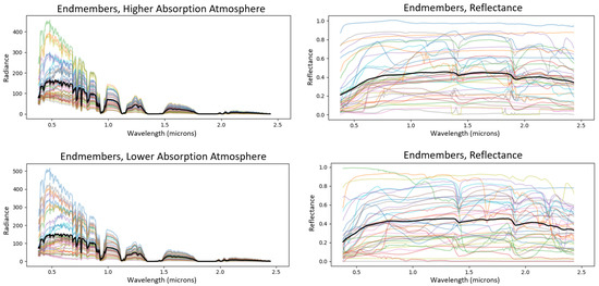
Figure 3.
At-sensor radiance for 39 spectra and the mean plotted in black (left-hand plots) along with the true reflectance for these materials and the mean of their reflectance in black (right-hand plots). The top row of plots have an atmosphere with greater absorption and the bottom row has less absorption.
Figure 4 shows reflectance and radiance values from different endmember means, showing that there is significant variation in both the radiance and reflectance values for different groupings of endmembers and atmospheres. These plots indicate the error in QUAC assumption Q3, that the mean of a group of reflectance spectra is constant.
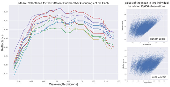
Figure 4.
The mean reflectance spectrum for 10 different groupings of spectra (left) and the reflectance and radiance values in two different bands for the mean from 15,000 of our observations.
2.2. Gaussian Process Atmospheric Compensation
The Gaussian process model can be described using conditional probabilities as follows. Let denote the dimensional vector of values for the mean of a set of radiance endmembers, and let be the dimensional mean vector of the reflectance for these endmembers. Let be the dimensional concatenation of and ,
We use capital letters , , and for the arrays consisting of k observations of each type, which are of size , , and respectively.
Making the assumption that is a multivariate normal random variable, we can compute the mean and covariance . Let and be the means for the radiance and reflectance so that is the concatenation of and . If we denote the covariance of the by , the covariance of by , and the covariance of by , then the covariance matrix can be written in block form as
Then for a given radiance which is the mean of endmembers, we get the conditional probability distribution for the reflectance as the multivariate normal distribution [8]
where
This conditional probability density function is depicted in the case where x is one dimensional and is two dimensional in Figure 5. The predicted mean reflectance is then the expected value of the reflectance given the observed radiance,
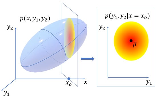
Figure 5.
The conditional probability density function for a multivariate normal distribution is a lower dimensional multivariate normal distribution.
Our description of a Gaussian processes (GP) model was in the context of predicting reflectance from radiance. More generally, GP is a machine learning method for predicting an output vector from an input vector in a Bayesian framework assuming the Gaussian probability distributions. It is often used for predicting financial or cyclical weather patterns from data, where the input is the value of some measurement over time, and the output is the values over a following set of times. It can be applied to any function of a continuous parameter (e.g., time or in our case wavelength) where the measured output value at any finite set of input parameter values is a multivariate Gaussian random variable. This includes the case of continuous input variables (infinite dimensions) but the computation is done on a discrete input parameters subset for obvious computational reasons.
This predicted mean reflectance can be used in atmospheric correction similar to how the ‘universal mean’ is used in QUAC, as follows. First, for each band the minimum value over all pixels in the image for that band is determined, and this minimum value is used as the offset, which is an estimate for the upwelling radiance. This offset is subtracted from every pixel in the image, and then a collection of endmembers is collected from the image. The mean of these endmembers is the radiance vector , and the predicted reflectance is . The gain for the atmospheric conversion is , which is multiplied per-band for every spectrum in the image to complete conversion to reflectance. We call this method of atmospheric correction GPAC (Gaussian Process Atmospheric Correction).
Two examples of mean of the radiance endmembers (left) and predicted reflectance from GPAC (right) are shown in Figure 6 using observations from our test data. Observe that the method accurately predicts the mean reflectance spectra even though these means differ from each other significantly. This enables us to perform accurate atmospheric correction in situations where the assumption in QUAC of a universal mean is not a reasonable assumption.
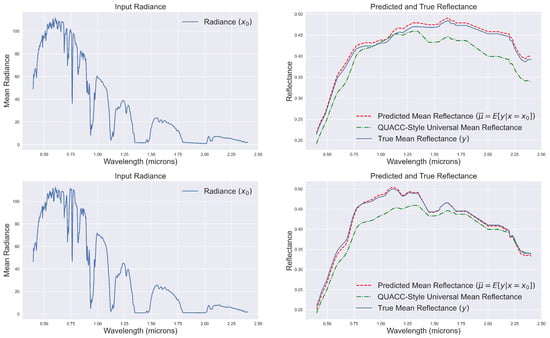
Figure 6.
(left) Two different mean radiance spectra for different endmember groups and different atmospheres. (right) The true mean reflectance for each endmember set, the GPAC predicted mean reflectance, and the QUAC-style universal mean. Observed that the GPAC predicted mean appears to be a better approximation to the actual mean.
The covariance matrices computed from the radiance and reflectance training data for the parameters computations in 1 are shown in Figure 7. From this figure we can see that is a covariance matrix for reflectance spectra, is a covariance for radiance spectra, and the off diagonal matrices indicate a conversion between units.
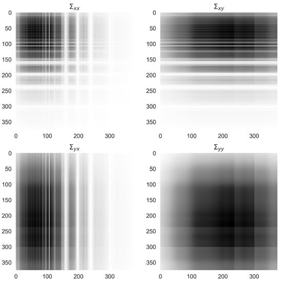
Figure 7.
The covariance matrices computed from the radiance and reflectance data for the parameters for the conditional probability.
An advantage of the conditional probability in the Gaussian process is that we can unpack the model to determine what it is learning. This method is not a black box. In Figure 8, we plot the first four eigenvectors of the covariance matrix along with transmittance spectra. These eigencvectors show that the conditional probability is learning variation in the transmittance for atmospheres of varying physical properties.
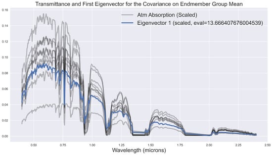
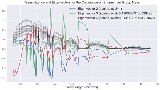
Figure 8.
The transmittance for various atmospheres plotted along with the first eigenvector (top) and the next three eigenvectors (bottom) for the matrix .
2.3. Denoising Autoencoder Atmospheric Compensation
An autoencoder is a deep learning neural network that passes data through a series of layers that decrease in size leading to a dimensionally smaller representation of the data (encoding), and then passing the lower dimensional representation through a symmetric series of layers back to the original data shape (decoding). When trained well, the process learns a representation of the data in the reduced dimensional space so that the encoding stage removes noise and the decoding stage recovers the data in the original space [9,10,11,12]. A diagram of the architecture of our autoencoder is shown in Figure 9.
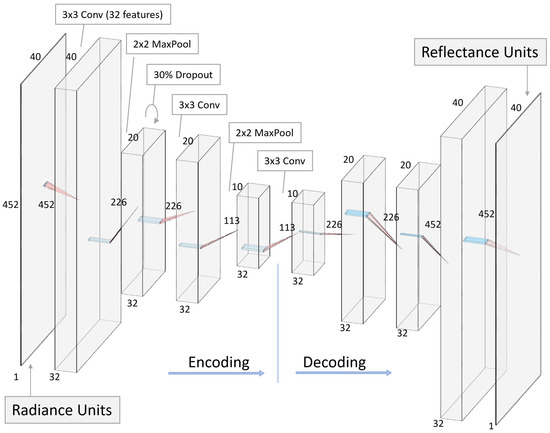
Figure 9.
The autoencoder neural network used for converting from radiance to reflectance. Details for the network architecture are included in the labels.
Our autoencoder is trained on the reflectance and radiance data described previously (removing the last 3 bands to provide an appropriate even number for the autoencoder), providing the full 2-D array of endmembers and mean for each rather than just the mean. One training data observation with both radiance (input for the autoencoder) and reflectance (output) is shown in Figure 10. All of our data and methods are provided open access (https://www.kaggle.com/code/billbasener/autoencoder-atmospheric-compensation/notebook, https://github.com/wbasener/DeepLearningAtmosphericCompensation/, accessed on 23 December 2022).
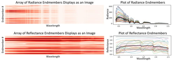
Figure 10.
The training data for the auto encoder is an array of the radiance endmembers (upper-left) and array of the reflectance endmembers (lower-left). The plots for each of these is shown to the right.
3. Results
We tested all three methods: Gaussian Process Atmospheric Compensation (GPAC), Universal Mean Regression (UMR), and our Denoising Autoencoder (DA) for atmospheric correction on our test data. The data consisted of 100,000 observations, where each observation has an X input array of 40 radiance spectra and a Y output variable of these 40 spectra in reflectance. The radiance was created from the reflectance by applying a MODTRAN atmospheric absorption. For each observation, the reflectance spectra were a random selection from a library of over 1000 spectra and the parameters for the MODTRAN atmosphere were randomly selected. The data was randomly split into 66,667 training observations and 33,333 test observations. The test set is then unique radiance-reflectance pairs of spectra (We exclude the mean for scoring, so each group has 39 rather than 40). The radiance spectra generated by this process are an approximation to at-sensor radiance minus the offset. This offset is often approximately removed via dark pixel subtraction in practice, so we focus on measuring the prediction of the gain.
Evaluation Metrics
The GPAC and DA methods are the novel methods described in Section 2, and the UMR method is what is used within the QUAC atmospheric correction process to estimate reflectance from sensor radiance minus the offset. We applied each method to the radiance spectra in each test observation to determine predicted reflectance spectra. (The GPAC and UMR methods each produce a mean reflectance which is used to determine a gain, which is then applied to each radiance spectrum to obtain the reflectance, while the DA directly provides a predicted reflectance for each radiance spectrum.) We then computed the following metrics.
- 1.
- Mean Correlation: The mean of the correlations between each predicted reflectance spectrum with the corresponding true reflectance.
- 2.
- Standard Deviation in Correlation: The standard deviation of the correlations between each predicted reflectance spectrum with the corresponding true reflectance.
- 3.
- Percent with all bands in of True: The percent of spectra (out of the 1,299,987) for which the predicted reflectance is within of the true reflectance for all bands.
- 4.
- Percent with of bands in of True: The percent of spectra (out of the 1,299,987) for which the predicted reflectance is within of the true reflectance for at least of the bands.
The mean correlation between the predicted and true spectra is an important metric because most material detection and identification process incorporate correlation (in native or PCA space), and moreover the chemical bonds in materials appear as features (minima, maxima, slopes, etc.) in the spectra, and correlation between spectra captures these better than absolute difference. It is clear from our test that the GPAC method provides the most accurate (highest mean) and most consistent (lowest standard deviation) results when measured by correlation between predicted reflectance and true reflectance.
The two metrics measuring how well the predicted reflectance stays within plus or minus of the true reflectance provide additional import information on accuracy. This type of comparison has been used to justify the accuracy of QUAC [7]. Often, the predicted reflectance will be close to the true reflectance except for a small number of bands near the water band regions, where high absorption from a particular atmosphere can result in low signal in the radiance spectra and unnaturally high values in predicted reflectance for GPAC and UMR. The GPAC method performed the best by these metrics as well. Notably, for of spectra the predicted reflectance with was within of the true reflectance for at least of the bands, while this was true for UMR for only of the spectra.
Six reflectance endmembers along with their approximated reflectance from GPAC are shown for two different observations sets in Figure 11. Observe that along the edges of the water band regions, that 1/SNR (where SNR for a bands is the max radiance over all bands divided by the radiance value for band ) is higher and there are poor approximations for the individual bands. This is a common problem that arises in atmospheric correction methods when the low SNR water bands result in poor reflectance estimates.
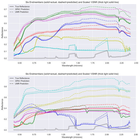
Figure 11.
For two different observation endmeber sets and atmospheres, the true and predicted (using GPAC and UMR) reflectance spectra for six endmembers are shown. Also shown is 1/SNR for each band, with the SNR is the radiance value for the given band divided by the maximum radiance.
The results in Figure 11 show results from atmospheric correction using the GPAC that are more accurate than using the QUAC-style universal mean regression prediction. For example, in the upper plot observe that the UMR reflectance are close approximations up to about 1.2 microns, then there are unrealistic features in the 1.2 to 1.5 micron range, and then a growing over-approximation of the reflectance from 1.75 on. in the lower plot, the universal mean regression prediction has an unrealistic feature created around 0.55–0.9 microns, and as previously an over-approximation of the reflectance from 1.25 microns on, which seems to increase with increasing wavelength. These observations are all consistent with the results of Table 1.

Table 1.
Evaluation metrics for the Gaussian P Atmospheric Correction (GPAC), Universal Mean Regression (UMR), and Denoising Autoencoder (DA) methods.
Two different sets of 40 endmembers in reflectance and as predicted by the denoising autoencoder are shown in Figure 12. Observe that the difference between the true and predicted reflectance are significant in comparison to the differences shown in Figure 11. The predicted spectra from the denoising autoencoder differ in both value and first derivative in comparison to true spectra.
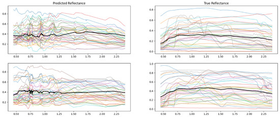
Figure 12.
Two different sets of 40 endmembers in reflectance (right) and as predicted by the denoising autoencoder (left).
4. Conclusions
The most common automated atmospheric compensation method is QUAC [5], described in Section 1. In this method, after estimating and removing an offset (upwelling diffuse), a set of endmembers is selected and the UMR method is used to estimate a gain (transmittance), which is then applied to the whole image. Some additional heuristics are used, such as excluding vegetation or mud from the endmembers and choosing a subset of bands for endmember selection. This universal mean is shown in Figure 4 of [5] and its use in regression is shown in Equation (3) in [5]. Despite the approximations, this method generates reasonable reflectance spectra that are with of those generated with physics-based methods such as FLAASH [7].
4.1. Gaussian Process Atmospheric Compensation
The theoretical design of the Gaussian process mean from GPAC should be a better approximation to the mean reflectance of a set of endmembers than a constant universal mean, and our test indicates that this is robustly true. While we trained and tested on MODTRAN data rather than image data, we expect that incorporating GPAC in place of UMR in QUAC would provide substantial significant robust improvement in atmospheric compensation.
4.2. Denoising Autoencoder Atmospheric Compensation
While our denoising autoencoder method does not perform well in comparison to the other methods we tested, we believe that it is an important first step in applying the growing field of deep learning of physical principles to atmospheric compensation in hyperspectral imagery and remote sensing. The challenge with the denoising autoencoder (and a challenge with neural networks in general) is that the network has a very high variance. That is, there is very large variance in what types of functions (from radiance to reflectance) that can be learned by the model. This is evident in Figure 12, which shows that the resulting predictions that do not retain the shape or derivatives of true reflectance spectra.
We expect, based on the trajectories of other efforts in deep learning of physical phenomena, that better inclusion of physical principles in the architecture of the autoencoder could substantially improve the quality of output. For example, the inclusion of skip connections in the ResNet Network enables layers that learn functions closer to the identity, leading to the ability to train much larger, more complex, networks [13] with a smoother loss function that has fewer local minima [14]. It is possible that similar architecture modifications, or maybe a hybrid approach with a Gaussian process, could aid a deep learning model to approximate the physics involved and/or train to learn the physics better.
5. Patents
The University of Virginia is considering filing a patent based on the GPAC method described in this paper.
Author Contributions
Conceptualization, B.B. and A.B.; QUAC software written in C++, A.B.; validation, A.B. and B.B.; formal analysis, B.B. and A.B.; data curation, B.B.; writing—original draft preparation, B.B.; writing—review and editing, B.B. and A.B.; visualization, A.B. and B.B.; supervision, B.B. All authors have read and agreed to the published version of the manuscript.
Funding
This research received no external funding.
Data Availability Statement
Code in Python for all algorithms in this paper are available at https://www.kaggle.com/code/billbasener/autoencoder-atmospheric-compensation/notebook. Some data is available with that resource, but some reflectance spectra used are not in the public domain. The MODTRAN coefficients can be accessed via http://modtran.spectral.com/ and http://modtran.spectral.com/modtran_home.
Conflicts of Interest
The authors declare no conflict of interest.
Abbreviations
The following abbreviations are used in this manuscript:
| MDPI | Multidisciplinary Digital Publishing Institute |
| MODTRAN | MODerate resolution atmospheric TRANsmission |
| GPAC | Gaussian Process Atmospheric Correction |
| UMR | Universal Mean Regression |
| DA | Denoising Autoencoder |
References
- Berk, A.; Conforti, P.; Kennett, R.; Perkins, T.; Hawes, F.; van den Bosch, J. MODTRAN6: A major upgrade of the MODTRAN radiative transfer code. In Algorithms and Technologies for Multispectral, Hyperspectral, and Ultraspectral Imagery XX; Velez-Reyes, M., Kruse, F.A., Eds.; International Society for Optics and Photonics (SPIE): Bellingham, DC, USA, 2014; Volume 9088, p. 90880H. [Google Scholar]
- Perkins, T.; Adler-Golden, S.M.; Matthew, M.W.; Berk, A.; Bernstein, L.S.; Lee, J.; Fox, M. Speed and accuracy improvements in FLAASH atmospheric correction of hyperspectral imagery. Opt. Eng. 2012, 51, 1–8. [Google Scholar] [CrossRef]
- Mamaghani, B.G.; Sasaki, G.V.; Connal, R.J.; Kha, K.; Knappen, J.S.; Hartzell, R.A.; Marcellus, E.D.; Bauch, T.D.; Raqueño, N.G.; Salvaggio, C. An initial exploration of vicarious and in-scene calibration techniques for small unmanned aircraft systems. In Autonomous Air and Ground Sensing Systems for Agricultural Optimization and Phenotyping III; International Society for Optics and Photonics: Bellingham, DC, USA, 2018; Volume 10664. [Google Scholar]
- Gao, B.; Montes, M.J.; Davis, C.O.; Goetz, A.F.H. Atmospheric correction algorithms for hyperspectral remote sensing data of land and ocean. Remote Sens. Environ. 2009, 113, S17–S24. [Google Scholar] [CrossRef]
- Bernstein, L.S.; Jin, X.; Gregor, B.; Adler-Golden, S.M. Quick atmospheric correction code: Algorithm description and recent upgrades. Opt. Eng. 2012, 51, 1–12. [Google Scholar] [CrossRef]
- Katkovsky, L.V.; Martenov, A.O.; Siliuk, V.A.; Ivanov, D.A. SHARC method for fast atmospheric correction of hyperspectral data. In Remote Sensing of Clouds and the Atmosphere XXIII; Comerón, A., Kassianov, E.I., Schäfer, K., Picard, R.H., Weber, K., Eds.; International Society for Optics and Photonics (SPIE): Bellingham, DC, USA, 2018; Volume 10786, pp. 53–65. [Google Scholar]
- Bernstein, L.S.; Adler-Golden, S.M.; Sundberg, R.L.; Levine, R.Y.; Perkins, T.C.; Berk, A.; Ratkowski, A.J.; Felde, G.; Hoke, M.L. Validation of the quick atmospheric correction (quac) algorithm for vnir-swir multi-and hyperspectral imagery. In Algorithms and Technologies for Multispectral, Hyperspectral, and Ultraspectral Imagery XI; SPIE: Bellingham, DC, USA, 2005; Volume 5806, pp. 668–678. [Google Scholar]
- Eaton, M.L. Multivariate Statistics: A Vector Space Approach; John Wiley & Sons, Inc.: New York, NY, USA, 1983. [Google Scholar]
- Bank, D.; Koenigstein, N.; Giryes, R. Autoencoders. arXiv 2020, arXiv:2003.05991. [Google Scholar]
- Vincent, P.; Larochelle, H.; Bengio, Y.; Manzagol, P. Extracting and composing robust features with denoising autoencoders. In Proceedings of the 25th International Conference on Machine learning, Helsinki, Finland, 5–9 July 2008; pp. 1096–1103. [Google Scholar]
- Vincent, P.; Larochelle, H.; Lajoie, I.; Bengio, Y.; Manzagol, P.; Bottou, L. Stacked denoising autoencoders: Learning useful representations in a deep network with a local denoising criterion. J. Mach. Learn. Res. 2010, 11, 12. [Google Scholar]
- Ruikai, C. Research progress in image denoising algorithms based on deep learning. J. Phys. Conf. Ser. 2019, 1345, 042055. [Google Scholar] [CrossRef]
- He, K.; Zhang, X.; Ren, S.; Sun, J. Deep residual learning for image recognition. In Proceedings of the IEEE Conference on Computer Vision and Pattern Recognition, Las Vegas, NV, USA, 27–30 June 2016; pp. 770–778. [Google Scholar]
- Li, H.; Xu, Z.; Taylor, G.; Studer, C.; Goldstein, T. Visualizing the loss landscape of neural nets. Adv. Neural Inf. Process. Syst. 2018, 31, 3144. [Google Scholar]
Disclaimer/Publisher’s Note: The statements, opinions and data contained in all publications are solely those of the individual author(s) and contributor(s) and not of MDPI and/or the editor(s). MDPI and/or the editor(s) disclaim responsibility for any injury to people or property resulting from any ideas, methods, instructions or products referred to in the content. |
© 2023 by the authors. Licensee MDPI, Basel, Switzerland. This article is an open access article distributed under the terms and conditions of the Creative Commons Attribution (CC BY) license (https://creativecommons.org/licenses/by/4.0/).