Article

Digital Mapping of Root-Zone Soil Moisture Using UAV-Based Multispectral Data in a Kiwifruit Orchard of Northwest China

1
State Key Laboratory of Hydraulics and Mountain River Engineering & College of Water Resource and Hydropower, Sichuan University, Chengdu 650065, China
2
College of Resources and Environment, University of Electronic Science and The Technology of China, Chengdu 611731, China
3
Department of Land Air & Water Resources, University of California, Davis, CA 95616-5270, USA
*
Author to whom correspondence should be addressed.
Remote Sens. 2023, 15(3), 646; https://doi.org/10.3390/rs15030646
Submission received: 21 December 2022 / Revised: 16 January 2023 / Accepted: 18 January 2023 / Published: 21 January 2023

Abstract

:
Accurate estimation of root-zone soil moisture (SM) is of great significance for accurate irrigation management. This study was purposed to identify planted-by-planted mapping of root-zone SM on three critical fruit growth periods based on UAV multispectral images using three machine learning (ML) algorithms in a kiwifruit orchard in Shaanxi, China. Several spectral variables were selected based on variable importance (VIP) rankings, including reflectance Ri at wavelengths 560, 668, 740, and 842 nm. Results indicated that the VIP method effectively reduced 42 vegetation indexes (VIs) to less than 7 with an evaluation accuracy of root-zone SM models. Compared with deep root-zone SM models (SM40 and SM60), shallow root-zone SM models (SM10, SM20, and SM30) have better performance (R2 from 0.65 to 0.82, RRMSE from 0.02 to 0.03, MAE from 0.20 to 0.54) in the three fruit growth stages. Among three ML algorithms, random forest models were recommended for simulating kiwi root-zone SM during the critical fruit growth period. Overall, the proposed planted-by-planted root-zone SM estimation approach can be considered a great tool to upgrade the toolbox of the growers in site-specific field management for the high spatiotemporal resolution of SM maps.

Graphical Abstract

1. Introduction

The cultivation of kiwifruit, one of the world’s major cash crops, helps promote economic development in northwest China, northeast New Zealand, and Italy [1]. In recent years, the kiwifruit industry has grown to become the dominant agricultural industry and the second-largest fruit industry in Shaanxi, NW China [2]. The soil moisture (SM) measurement provides information about the available water for tree roots, which is crucial for determining plant growth [3,4]. For accurate irrigation management, timely and accurate SM estimation can be helpful in monitoring soil moisture status of kiwi during the critical growth season [5]. In order to assess the drought situation in the orchard and measure water movement in the soil, it is crucial to determine the high-precision spatial mapping of root-zone SM according to the orchard irrigation unit. Meanwhile, it is also an essential prerequisite for timely and accurate monitoring of orchard irrigation and fruit growth management throughout the growing period. Therefore, a precise planted-by-planted high-resolution spatial mapping of root-zone SM is essential for monitoring kiwifruit canopy water content and canopy vitality, estimating production, and planning irrigation.
The current traditional method for measuring SM in the field is to dry soil samples and then calculate their water content in the lab. They will, however, destroy the roots of trees at a high cost and with low efficiency [6]. Furthermore, laboratory-based SM relies on point measurements that ignore spatial and temporal variability as opposed to field measurements as remote sensing (RS) technology, high-precision sensors, and multiple-sensor integrated system advance, unmanned aerial vehicles (UAVs) offer a practical way to describe virtually every aspect of plant physiology accurately and nondestructively. By combining various spectral bands, vegetation indexes (VIs) are derived, which are commonly used for estimating vegetation structure or agronomic parameters [7,8,9,10]. Several researchers have also conducted numerous constructive investigations into the sensitivity of SM and spectral reflectance [7,11,12,13]. In most of these studies, however, the surface soil water content of farmland or underlying areas was estimated. Cheng et al. [14] evaluated the SM simulated by multimodal data fusion and confirmed that VIs based on multispectral (MS) data could obtain high-accuracy estimates of SM. In Romero et al.’s [15] paper, VIs calculated from MS imagery were used to estimate vine water status using a pattern recognition algorithm, and results indicated that optimized soil-adjusted vegetation index (OSAVI) was an outstanding predictor of vine water status. Furthermore, a few studies focused on estimating root-zone SM in a kiwi orchard using pure kiwi canopy reflectance. Through pretreatment, external noise is eliminated, pure canopy spectral features are enhanced, nonlinear relationships are boosted, and specific target model accuracy is improved [16,17,18]. By using the variable projection importance (VIP) function from the partial least squares (PLS) method to optimize pure kiwi canopy spectral indices, more feature VIs could be detected, and the correlation between root-zone SM of kiwifruit and spectral characteristics of a target could be improved.
Several mainstream models of machine learning (ML) algorithms, such as decision trees, neural networks, support vector machines (SVMs), and clustering, have made it possible to estimate SM from spectral reflectance data [19,20,21]. ELM is one of the simplest and fastest neural network algorithms, and it is excellent at generalizing and migrating [22]. Peng et al. [23] found that ELM had the best overall performance among the three ML models for predicting nutrients in the grape canopy. In the meantime, numerous studies have been conducted that the SVMs and the RF method are excellent ensemble-learning algorithms with fewer input training parameters and higher robustness [24,25,26]. These algorithms have good evaluation performance on plant conditions, such as the nutritional status [27,28], canopy water content [29,30], biomass [31], and chlorophyll content [32]. However, few studies have estimated root-zone SM in kiwi trees based on UAV MS data. Moreover, the majority of studies ignore various spectral information of red-edge bands in favor of measuring only the usual spectral variable before making predictions. Therefore, multiple sensitive vegetation indices with the red-edge band, as well as commonly used three efficient ML methods, were adopted in this study to improve UAV MS imagery diagnoses of root-zone SM in the kiwifruit orchard.
Crop mapping data were traditionally collected via statistical reports, inventory records, or in-person field inspections. Remote sensing (RS) now significantly simplifies this labor- and time-consuming task. With the advancement of RS technology, the UAV field has grown rapidly, providing high spatial-resolution images. Furthermore, UAVs are versatile enough to contribute to a wide range of data collection operations without specific climate limitations [33]. The benefit of using UAVs to map crop areas is that it allows farmers to check their fields on a regular basis. Furthermore, UAV imagery analytics provide more information on farmlands than just cultivated crop types and field acreage. In precision agriculture, UAVs equipped with various sensors are commonly used to report on vegetation health, such as plant structure, chlorophyll content, and soil properties [34]. In spite of several studies that have estimated vegetation or soil attributes from UAV images, the orchard planting scale is rarely used to estimate the root-zone SM of kiwi trees.
This study aims to implement planted-by-planted spatiotemporal monitoring of root-zone SM on three critical fruit growth periods in the kiwifruit orchard, as well as to provide a new idea for precise irrigation decision-making during the entire fruit growth period of kiwi. Overall, the primary goals of this research are to (a) assess the root-zone SM through VIs calculated from SVM-extracted pure kiwifruit canopy MS data fusion and three ML algorithms, including RF, SVM and ELM; (b) determine whether the VIP sensitive variable selection method can reduce the input VI variables while ensuring the inversion accuracy of SM model; (c) investigate how critical period of fruit growth and soil depth affect the accuracy of SM estimation; (d) carry out planted-by-planted high-precision spatial mapping of root-zone SM combined with kiwi planting units.

2. Materials and Methods

2.1. Test Site and Experimental Setup

We conducted UAV-based surveys over three hectares of Actinidia chinensis var. deliciosa ‘Xuxiang’ at the kiwifruit orchard (34.241°N 108.164°E, 400 m above the sea level) of Wugong County, Xianyang City, Shaanxi Province, NW China (Figure 1A,B). This 8-year-old orchard was planted under a pergola of 2 × 4 m with drip irrigation (Figure 1C). In this region, the average temperature in July is 27.1 °C, with the coldest month being January at 1.65 °C. The average precipitation is 552.60–663.9 mm per year.
Due to the higher water requirements of kiwifruit throughout its entire growing season, we planned to conduct inversion studies on the root-zone SM during three critical kiwifruit’s growth seasons: the young fruit stage (Stage I), the fruit expansion stage (Stage II), and the mature fruit stage (Stage III). According to the analysis of soil texture, the soil of 0–40 cm in the study area is medium loam, and the soil below 40 cm is heavy loam, which has strong water retention and poor permeability. The soil bulk density of 0–30 cm, 30–40 cm, and 40–60 cm were 1.50 ± 0.02 g/cm3, 1.56 ± 0.05 g/cm3, and 1.70 ± 0.03 g/cm3, respectively. The field water capacities (θfc, the soil volumetric water content) of kiwifruit trees was 34.70 ± 0.15% at the 0–60 cm soil layer in 2021. Irrigation was limited to 65–70% (65% at Stages I and II, 70% at Stage III) and 95% θfc, respectively. Data from this study were all collected 1–2 days before each irrigation. Figure 2 depicts the meteorological data collected during the sampling period. The average temperature was 20.7 °C (range:16.7–24.1 °C), 25.6 °C (range: 17.1–31.2 °C), and 21.5 °C (range:17.8–25.3 °C) at Stage I, Stage II, and Stage III in 2021, respectively. Meanwhile, no irrigation events occurred on May 20, August 15, and September 9, and the precipitation was 35.8 mm, 23.2 mm, and 8 mm, respectively. The irrigation amounts of Stage I, Stage II, and Stage III were 60.7 mm/hm2 (1 time), 377.4 mm/hm2 (7 times), and 60.7 mm/hm2 (1 time), respectively.

2.2. Data Acquisition

Kiwifruit requires more water than other fruit trees since its low drought tolerance. Thus, it is required to manage the irrigation time of kiwifruit in the correct period of scientific irrigation. Furthermore, the root zone of kiwifruit was mainly distributed in the depth of 0–60 cm. As a result, at Stage I, Stage II, and Stage III, we collected five depths of root-zone SMs with 0–10 (SM10), and 10–20 (SM20). 20–30 (SM30), 30–40 (SM40), and 40–60 (SM60) cm, as well as UAV MS images.

2.2.1. SM Field Data Collection

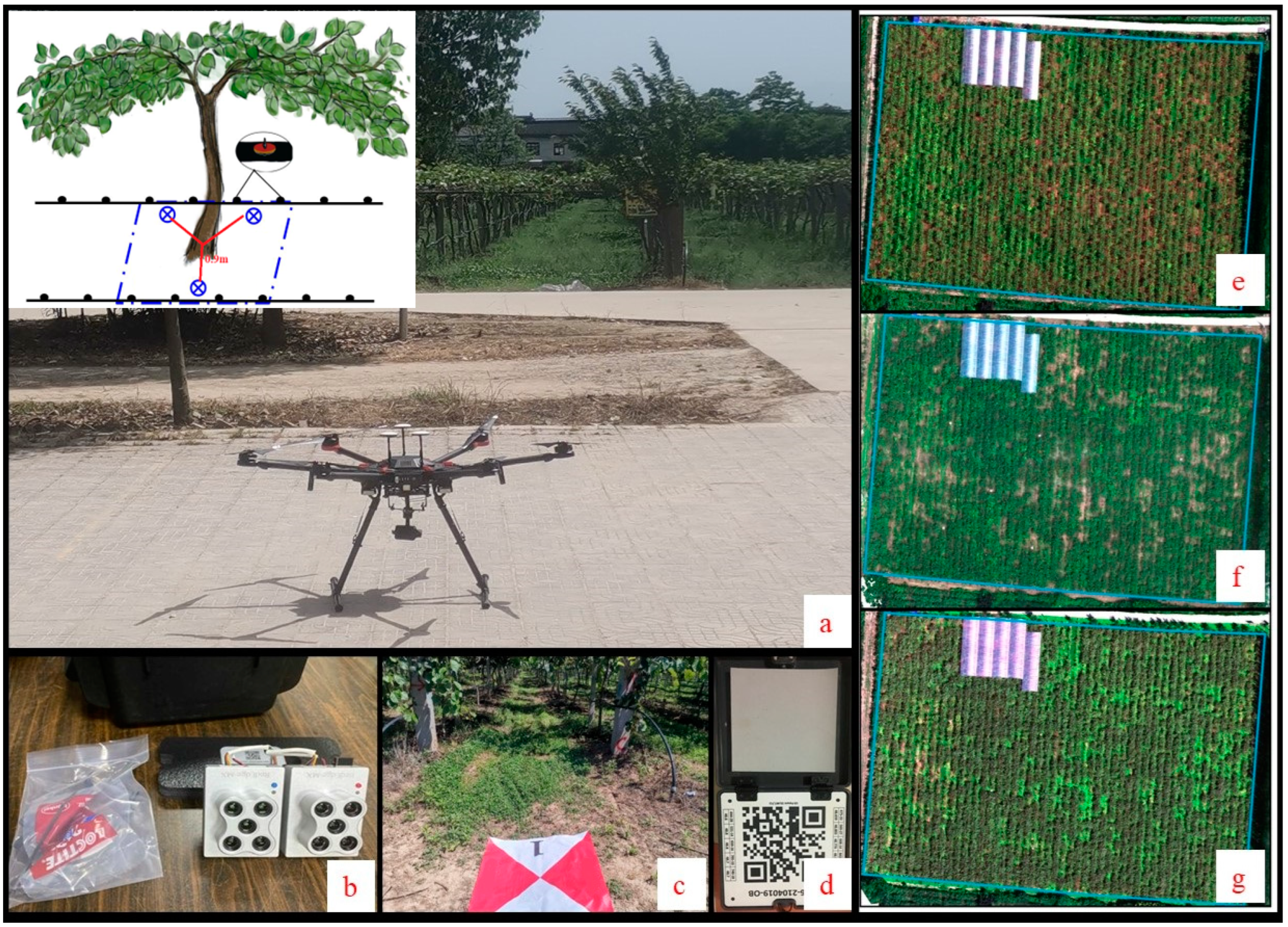
We set 100 fixed-point monitoring points (2.0 m * 4.0 m in Figure 1) according to the planting unit for synchronous data collection with the UAV flights. The 0–60 cm is the main distribution area and water absorption area of the kiwi root, so the sampling depth was determined to be 0–60 cm. The soil is stratified and sampled, which is divided into 5 layers (0–10 cm, >10–20 cm, >20–30 cm, >30–40 cm, >40–60 cm). The SM data were measured by FDR-TRIME (IMKO micromodtechnik GmbH, Leeds, Germany). One to three pre-buried tubes were set up in three positions within the 90 cm horizontal range of the kiwifruit tree (Figure 3a), with a total of 172. Furthermore, the mean of multiple measuring tubes at the same sampling point was taken as the measured value. The FDR-TRIME needs to manually extend the instrument into the pre-buried tube measurement. However, some of the pre-buried tubes were damaged and not measured during the UAV fighting time. The effective data sets with complete root-zone SM data of each layer at Stage I, Stage II, and Stage III were 90, 91, and 85 groups, respectively. The data measured by FDR-TRIME were calibrated by the drying method and converted into soil volumetric water content according to bulk density. Therefore, the SM data we finally used were the calibrated FDR-TRIME volumetric water content data.

2.2.2. UAV Multispectral Image Acquisition and Preprocessing

To collect kiwi MS images in this study, we used a six-rotor DJI Matrice 600 pro UAV (Dajiang Innovation Technology Co.; Ltd.; Shenzhen, China) equipped with a ten-channel Red-Edge MX Dual camera (Mica Sense, Seattle, WA, USA) (Figure 3a,b). The multispectral camera had ten bands (see Table 1) and a resolution of 1280 × 960 pixels. At three critical growth stages, we conducted all UAV campaigns in clear skies and with no wind (between 10:30 and 13:30) (Figure 3e–g). In order to ensure successful image reconstruction, we set the image overlap rate at 50 m flight altitude as 80%. Besides, the real-time kinematic (RTK) system was used to measure the coordinates of ground control points installed at the test site (Figure 3c). In order to calibrate the UAV MS data, the reflectance values of ten targets (calibrated reflectance panel, Mica Sense, Seattle, WA, USA) were measured prior to each flight (Figure 3d). The ten bands of scattered RS images were computer synthesized to produce multipage images after the data collection process (.TIF) (Figure 3e–g).

2.3. Canopy Spectral Information Extraction

Identifying stump locations and determining canopy boundaries can be extremely challenging when conducting in-field UAV surveys over kiwi vines for the following reasons: (1) training systems for pergolas produce a flat, dense canopy, making it impossible to identify stumps; (2) two neighboring plants’ canopies overlap due to disordered growth of their shoots [35]; and (3) there are a variety of weeds, bare soil, and other ground object types in the UAV MS imagery, causing the problem mixed pixels in each sampling cells. For these reasons, a workflow diagram of kiwi canopy spectral information extraction and reflectance matrix of mean values rasterize extraction was applied to each single-band UAV MS orthomosaic (Figure 4a,b). In (a) Step I, the SVM classifier was employed to identify kiwifruit canopy, weeds, shadow, and bare soil in the UAV MS data. Create a mask layer of the kiwi canopy to exclude weeds, shadow, and bare soil pixels from all spectral features of UAV imagery (Table 2) for further processing. According to (b) Step II, the pure kiwi canopy MS data were clipped with rectangular masks (2 * 4 m), which were placed perpendicular to the planting line. To reduce the data in MS data, planted-based kiwi canopy reflectance values were averaged within the masked region, and the results were stored in a matrix associated with the masking center coordinates. Then in (c) Step III, these zonal statistics of masked MS images were utilized to calculate 42 VIs correlated with SM.

2.4. The Calculation of Spectral Indices

In addition to eliminating environmental noise, spectral index methods have a higher sensitivity than single bands. We chose several vegetation indices (VIs) which have been shown to correlate with SM in the literature (Table 2). Furthermore, various combinations of red-edge bands from the Red-Edge MX Dual camera (B7 and B9, see Table 1) were calculated to generate potential VIs (Table 2, VIs in this study are shown in red) as input variables for SM prediction; 42 VIs were selected in total, as shown in Table 2.

2.5. The Feature Selection of Vegetation Indices

Since the effects of different VIs on the predicted SM can be different, it is critical to rank the relative importance of individual parameters to the SM. We used the variable importance in projection (VIP) variable screening method, which is based on partial least squares (PLS), to select the top 7 characteristic vegetation indices. In this method, two principal components were extracted based on the PLS principle, and variables with larger contributions were retained. Then, the VIP values of each component are obtained by calculating the mean of the sum of squares of the predicted residual. The higher the score, the greater the contribution to covariance and the greater the importance. The following is the calculation formula for VIP:
V I P = m k = 1 i b k 2 w j k 2 / k = 1 i b k 2
where W j k is the j-th entry of vector, b k is the regression weight of the k-th hidden variable, b k = u k T t k .

2.6. SM Prediction Model Calibration and Validation

The 42 VIs in Table 2 were extracted from 100 sampling plots (Figure 1C) as a mask layer and then matched with the field-measured root-zone SM of each experimental plot. After removing the anomalies and missing SM values, we selected 90, 91, and 85 data sets with complete SM values at each layer at Stage I, Stage II, and Stage III, respectively. In total, 450, 455, and 425 root soil data were obtained for each of the three periods.
The fold cross-validation method has been widely used to evaluate ML models because it effectively prevents over-learning and under-learning. In this study, SM data of each layer were separated and divided into three groups randomly by using the randperm function. The last group was used for testing, while the other two were used for training the three ML models. The accuracy of the average estimate value was then calculated as the final result. For further evaluation of ML models, we used the input combination screened based on the VIP strategy to construct RF, SVM, and ELM models for estimating the SM of each layer.

2.6.1. RF Model

The RF is a multivariable, nonlinear statistical method which obtains several random samples through repeated bootstrapping, followed by decision-making trees. Based on these decision-making trees, we can predict the value of the dependent variable for regression problems. In order to perform regression simulation of this algorithm, we set the number of decision trees (ntree) at 100 and the number of random variables per node (mtry) at 5.

2.6.2. SVM Model

SVMs is a generalized linear classifier that classifies data according to supervised learning; Its decision boundary is the maximum-margin hyperplane for solving the learning sample. In our model, the penalty factor (c) and radial basis function parameter (g) were 4 and 0.8, respectively. Moreover, we chose the radial basis function (RBF) as SVM’s kernel function, and then this suitable support vector is used to construct the prediction model.

2.6.3. ELM Model

ELM is designed by Huang et al. [62] as a feedforward neural network algorithm with a single hidden layer and is mostly used for regression and classification. Unlike a general neural network, the weights of the ELM input layer and hidden layer nodes are randomly or artificially given. There is only one thing left to determine: the threshold of the hidden neurons. We chose the sigmoid function for activation, and there were 15 hidden layer nodes in this study.

2.6.4. Model Calibration and Evaluation

The determination coefficient (R2), relative root mean square error (RRMSE), mean absolute error (MAE), and global performance indicator (GPI) were used to assess the accuracy of the RF, SVM, and ELM model predictions. The higher values of R2 and the lower values of RRMSE and MAE indicate a better imitative effect and accuracy of the model in predicting SM. The following is the formula for the evaluation index:
R 2 = 1 i = 1 n ( y i y i ^ ) 2 i = 1 n ( y i y i ¯ ) 2
R M S E = i = 1 n ( y i ^ y i ) 2 n
R R M S E = R M S E y ¯ × 100 %
M A E = i = 1 n | y i ^ y i | n
G P I = j = 1 m α j ( C I j C I m e d i a n )
where y i , and y i ^ are the measured values and predicted values, respectively, of the SM (%); y ¯ is the mean value of the measured values; n is the number of samples. CImedian is the median of the corresponding parameter; m is the number of statistical indicators; α j it is equal to 1 for R2 and equal to −1 for RRMSE and MAE.

3. Results

3.1. Changes of Root-Zone Soil Moisture in Fruit Growth Stages

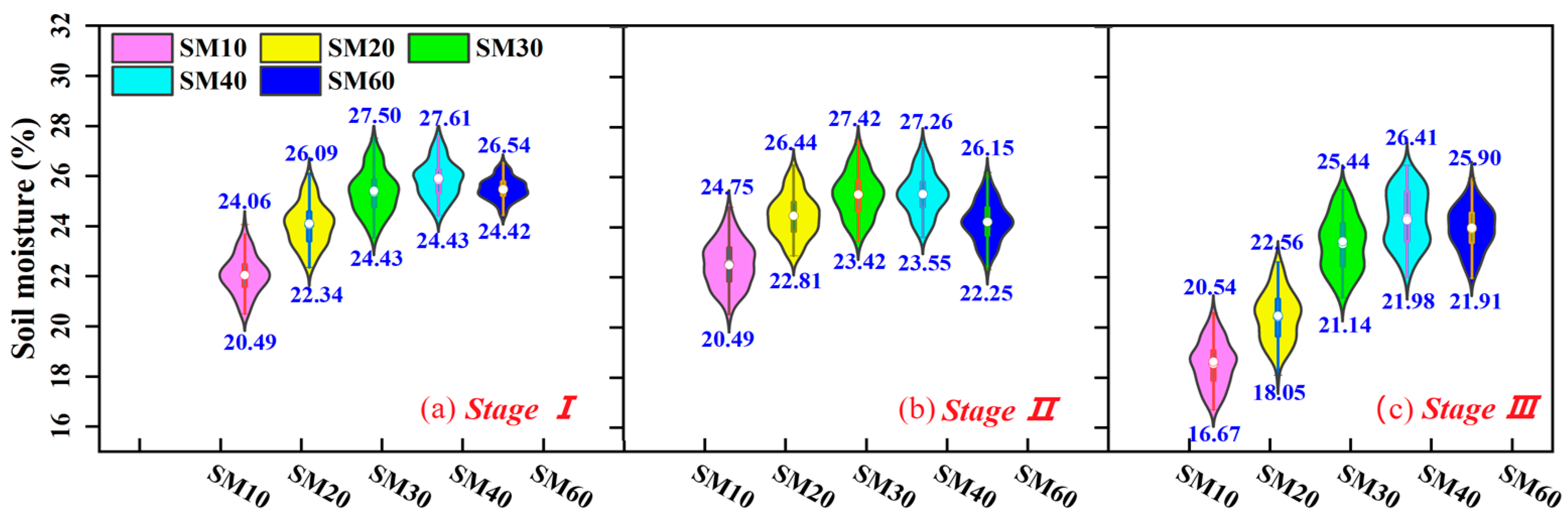
In Figure 5, the different root-zone SM values are shown for three key growth stages of the kiwifruit from May to September 2021. The distribution trend of SM characteristics in each layer of root-zone SM during the critical fruit growth period is relatively consistent, as can be seen. The SM increased and then decreased as the depth of the soil increased, reaching a maximum value of 21.98–27.61% at SM40. After reaching its peak, the SM60 (21.91–26.54%) remained relatively stable until the end of the critical fruit growing season. As a result, the deeper SM of kiwi is relatively less disturbed by the external environment, and the SM is basically saturated, where-as the soil water in the surface 0–20 cm changes significantly. Furthermore, results indicated that the difference of shallow root-zone SM (0–30 cm) value is large at Stage III, whereas it is relatively stable at Stage I and II, presumably due to the influences of irrigation, rainfall, and evapotranspiration during the critical kiwifruit growth season (from Figure 2). Stage III values ranged from 16.67–20.54%, 18.05–22.56%, and 21.14–25.44% for SM10, SM20, and SM30, respectively, while Stage I and Stage II values ranged from 20.49–24.75%, 22.34–26.44%, and 23.42–27.50% for SM10, SM20, and SM30, respectively. This suggested that there are differences in root-zone SM data applied in shallow root systems collected from three critical fruit growth seasons due to precipitation and other environmental influences.

3.2. Appropriate Spectral Indices for Soil Moisture Estimation

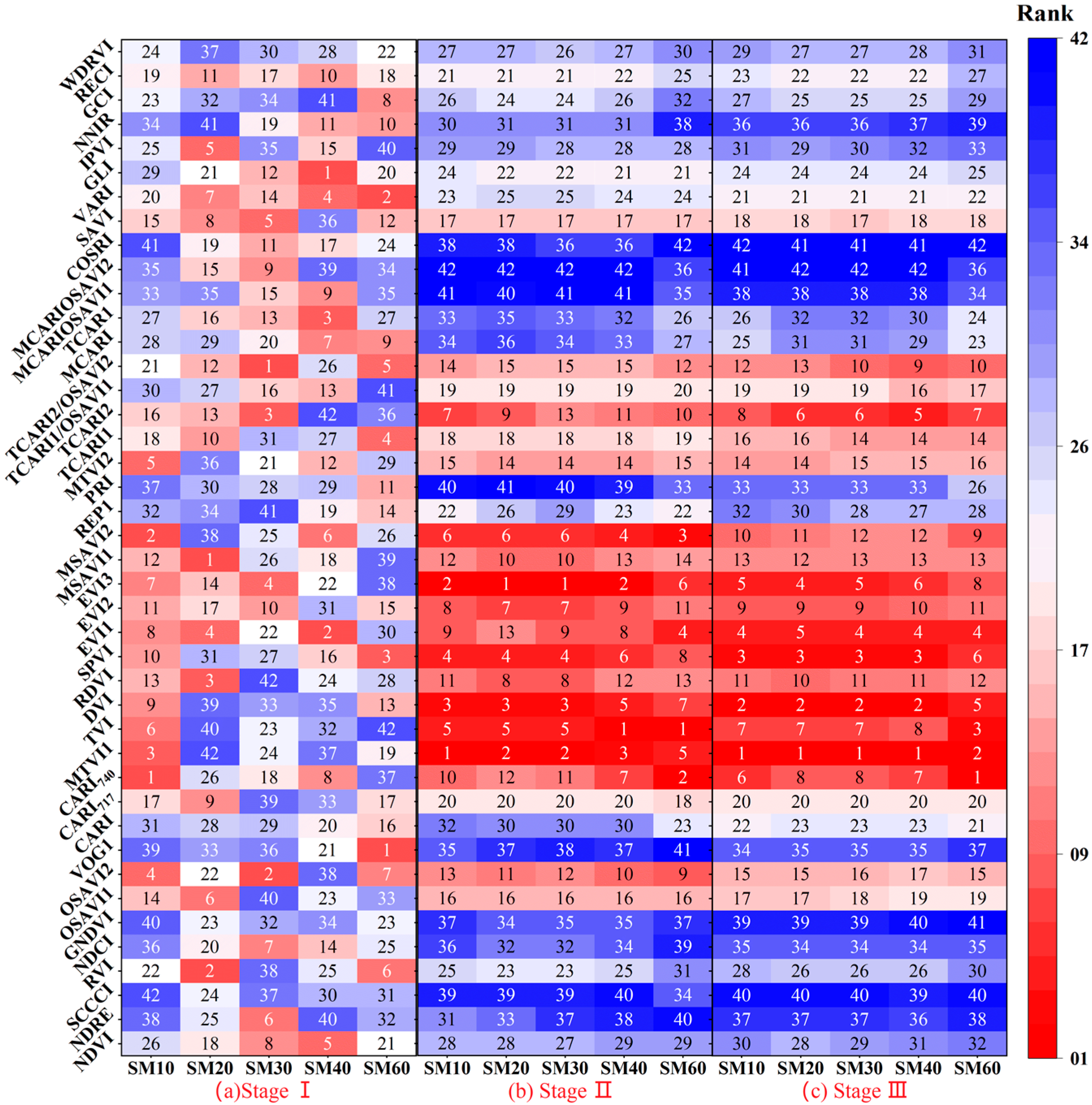
Several of the 42 spectral indices extracted from mask layers (Figure 4c) have multicollinearity, resulting in unstable analyses and incorrect predictions. Therefore, it was necessary to diagnose the relationship between the VIs and root-zone SM at various depths before training the models. In order to improve the stability of prediction, the VIP analysis was used in this study to reduce the dimensionality of the VIs (Figure 6). Our analysis was based on the calculated VIP value, and the top seven features (VIP > 1) were chosen as input parameters (Figure 6 and Table 3). According to our findings, the VIP ranking of SM at different depths at Stage I fluctuated significantly, similarly to Stage II and III. The results may be similar to the inversion of SM according to canopy VIs, while canopy growth would affect the inversion results. Thus, when canopy growth was slow at Stage I, SM at different depths had different sensitive VIs due to external influences. In Stage I, soil characteristic variables differ from layer to layer, as shown in Figure 6 and Table 3, but the selected variables are mostly related by CARI, TCARI, SAVI, OSAVI and MSAVI, MTVI and EVI, all of which were developed based on B4, B6, B9, and B10. In spite of that, each layer’s first seven indicators are still distinct at Stage II. It is noteworthy that the feature VIs selected by each layer are similar, such as EVI (EVI, EVI2, EVI3), MTVI (MTVI1 and MTVI2), and MSAVI (MSAVI1 and MSAVI2). As of Stage III, there were seven sensitive VIs per soil layer, including MTVI1, DVI, SPVI, EVI1, EVI3, TCARI2, and TVI. A notable finding was that CARI740 (referring to the conceptual framework of CARI, R740 was replaced by R700) appeared in the selected sensitive parameters for both SM60 and SM40.
According to the results, we found that kiwi canopy growth affects the canopy response characteristic when using the VI extracted from the canopy spectrum to recover root-zone SM. Generally, when a canopy grows strongly, each soil layer’s sensitive VIs become more consistent. Furthermore, the sensitive VI associated with SM at each stage was primarily CARI740, TCARI2, SAVI, OSAVI and MSAVI, MTVI (MTVI1 and MTVI2), EVI (EVI1 and EVI3) and TVI index, which were developed on the basis of B4, B6, B9, and B10 (Table 1 and Table 2).
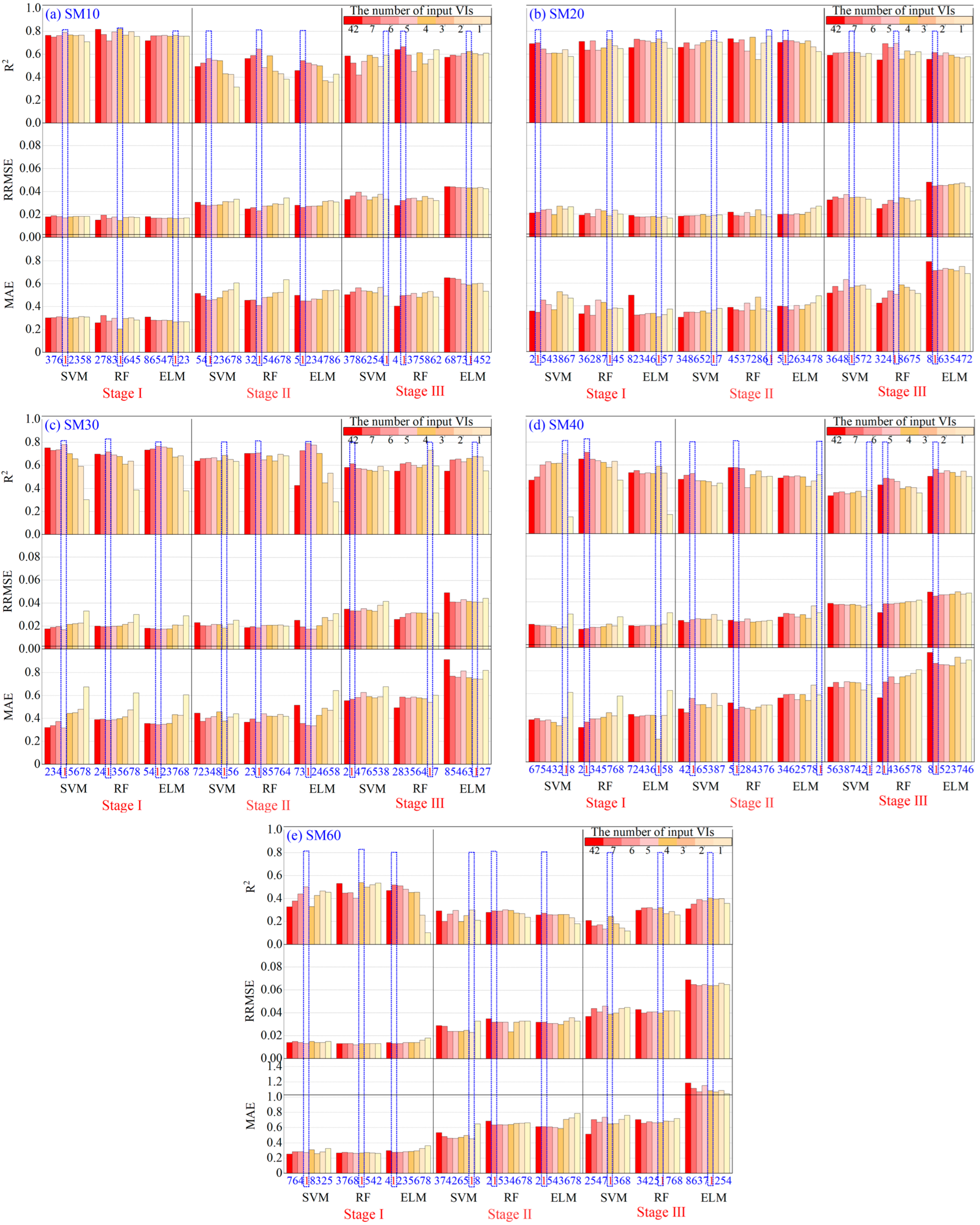
The accuracy evaluation of the three ML models for predicting root-zone SM (from SM10 to SM60) during three critical fruit growth periods is provided in Figure 7. These graphs showed the accuracy evaluation indexes of the SVM, RF, and ELM models under eight different input VI combinations. In each subgraph, it is indicated that the VIP variable selection method can effectively reduce the number of 42 VIs feature indices (R2 0.21–0.82) to less than 7 (R2 0.25–0.82) under the premise of ensuring the estimation accuracy of the SM model.
Moreover, among the 45 optimal models (ranked based on GPI), it is clearly indicated that the accuracy of the root-zone SM models applied at different root depths was in order of the shallow SM (SM10, SM20, and SM30)> the deeper SM (SM40 > SM60). The median R2 values for the SM10, SM20, SM30, SM40, and SM60 models were 0.67 (range: 0.54–0.82), 0.70 (range: 0.61–0.76), 0.72 (range: 0.61–0.79), 0.56 (range: 0.38–0.71) and 0.38 (range: 0.25–0.50), respectively, during the entire key growth season. The simulation error of the five models throughout the whole critical growth stage, with median RRMSE values of 0.03 (range: 0.01–0.04), 0.02 (range: 0.02–0.04), 0.02 (range: 0.02–0.04), 0.03 (range: 0.02–0.05) and 0.03 (range: 0.01-0.06), respectively. In addition, the median MAE values of each SM model were 0.41 (range: 0.20–0.59), 0.42 (range: 0.31–0.71), 0.44 (range: 0.32–0.74), 0.52 (range: 0.20–0.85) and 0.52 (range: 0.27–1.07), respectively.
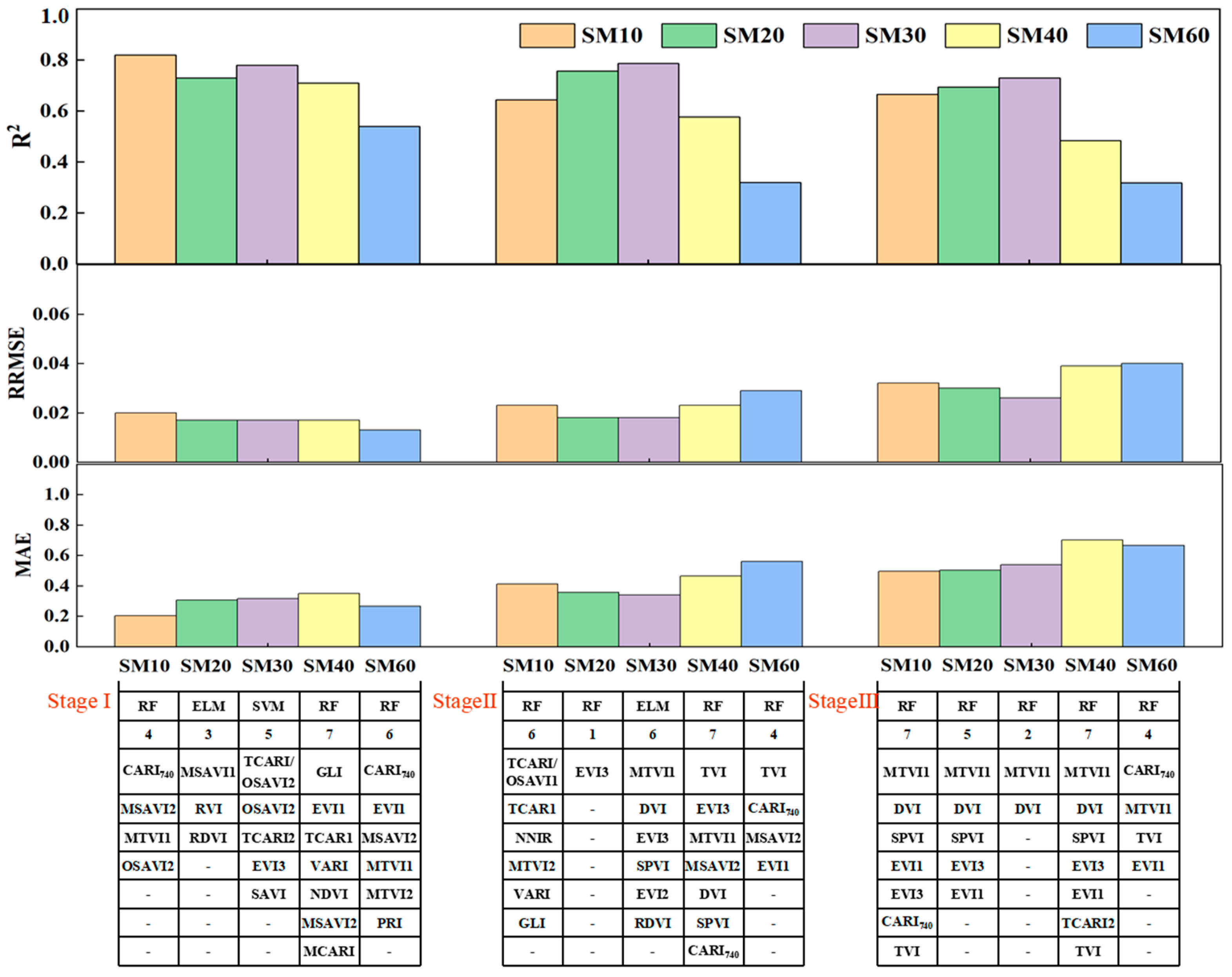
In addition, we also found that the inversion accuracy of root-zone SM models decreased at the progressive growth stage, while the inversion accuracy of SM20 and SM30 remained relatively stable throughout each growth period. Specifically, the median R2 values for the models at Stage I, Stage II, and Stage III were 0.69 (range: 0.50–0.82), 0.58 (range: 0.27–0.79), and 0.55 (range: 0.25–0.73), respectively. Moreover, the median RRMSE values of the models at three fruit growth stages were 0.02 (range: 0.01–0.02), 0.02 (range: 0.02–0.03), and 0.04 (range: 0.03–0.06), respectively. Comparisons of the MAE values also resulted in a similar conclusion, where the median MAE values 0.30 (range: 0.20–0.39), 0.44 (range: 0.34–0.60), and 0.65 (range: 0.49–1.07) during three critical growth periods, respectively. It is worth noting that the monitoring accuracy of SM10, SM20, and SM30 on the entire key fruit growth period was more accurate (R2 > 0.6, RRMSE < 0.032, MAE < 0.5), while the best monitoring period of SM40 and SM60 was only at Stage I, with R2, RRSME, MAE of 0.71, 0.02, 0.35, and 0.54, 0.01, 0.27, respectively.
Next, we examined the effect of the SVM, RF, and ELM algorithms on the different SM models during these critical fruit growth periods (Table 4, Table 5 and Table 6). Compared to SVM and ELM models, we found that the RF models exhibited relatively stronger robustness for SM prediction. At Stage I (Table 4), the R2 values for SM10, SM20, SM30, SM40, and SM60 models with the RF algorithm were increased by 4.05–7.32%, −0.81–3.86%, −6.54–8.33%, 0.0–20.92%, and 4.06–7.39%, respectively, compared with other two algorithms. Meanwhile, the R2 values for SM10, SM20, SM30, SM40, and SM60 models with the RF algorithm in Stage II were increased by 14.77–18.57%, 4.85–5.29%, −10.41–2.92%, 9.28–11.61%, and 7.36–18.45%, respectively (Table 5). At Stage III (Table 6), the R2 values for these five SM models with the RF algorithm were increased by 6.56–12.69%, 12.48–13.21%, 7.99–18.89%, −13.85–27.97% and −20.25–29.15% than other two algorithms, respectively. It is further found that the performance of RF algorithms only in a few SM models is unfavorable to ELM and SVM algorithms. However, the error values for the median RRMSE and MAE of SM models with RF, SVM, and ELM algorithms were 0.02, 0.03, 0.03, and 0.44, 0.45, and 0.51, respectively, during the critical fruit growth period. These data are consistent with the notion that the RF algorithms outperformed the other two models in terms of SM prediction robustness, with lower RRMSE and MAE, indicating heterosis performance across different root-zone SM.

3.3. Spatial Distribution of Root-Zone Soil Moisture in the Kiwi Field

The optimal prediction models of SM10, SM20, SM30, SM40, and SM60 on these key fruit periods were selected by GPI rankings shown in Figure 8. According to the prediction results at Stage I, the SM model developed by the RF algorithm with CARI740, MSAVI, MTVI1, and OSAVI2 variables had the best performance (Table 4). There was a higher R2 value than 0.8 and a low RRMSE value of 0.02, indicating that the model was reliable. In addition, the SM model in other layers in this period is better than that in the other two periods. Furthermore, the performance of SM20 and SM30 models were better than SM10 at Stage II and Stage III, which may be related to the higher weed cover in kiwifruit orchard at these stages. According to the model performance on three critical fruit growth periods for SM prediction (Figure 8), the SM10 model at Stage I outperformed the other two stages (highest R2 0.82, lowest RRMSE 0.02 and MAE 0.20), followed by SM20 and SM30 models (R2, RRMSE, MAE were in the range of 0.69–0.79, 0.02–0.03, 0.32–0.50, respectively, for the entire key growth season), whereas SM40 and SM60 exhibited diminished performance with lower R2 (0.32–0.54), higher RRMSE (0.01–0.06) and MAE (0.27–1.07). This is because the SM model based on optical RS in this study is mainly based on the average reflectance of kiwifruit canopy leaves. The absorption of water and nutrients by the canopy during the growth period of kiwifruit mainly depends on the root hair cells in the mature area of the root tip. The root hair area of kiwifruit is shallow, and it is widely distributed in the 0–30 cm soil layer. Therefore, the accuracy of the shallow SM model is high, and it performs better when the kiwifruit canopy is lush and healthy in Stages II and III. The deep root zone is the main root growth area of kiwifruit. There were fewer capillary roots in 30–40 cm and very few below 50 cm, which accounted for a small proportion of canopy water transport. Therefore, the performance of deeper SM models in this study was poor, and SM40 > SM60.
Overall, the RF is the most recommended model for estimating the kiwi root-zone SM, with fewer simple input parameters, higher simulation accuracy, and easy operation. Furthermore, the results of planted-by-planted spatial simulation of root-zone SM based on planting patterns can assist agricultural water managers in making irrigation decisions.
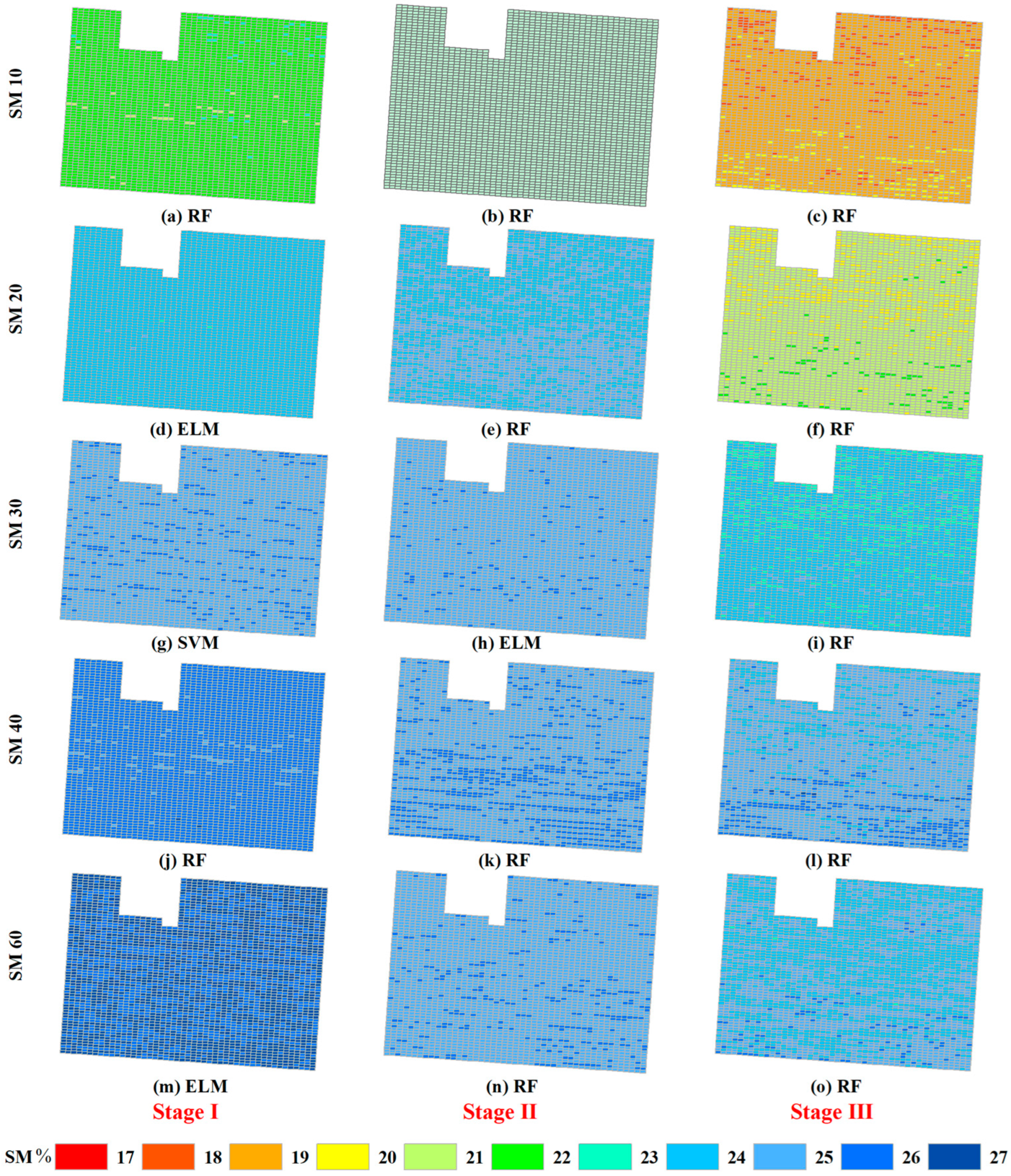
The planted-by-planted spatial distribution of root-zone SM prediction results on the critical fruit growth period based on the above optimal model is shown in Figure 9. The variation characteristics of SM during these critical fruit growth periods were similar to the measured values (Figure 5). Although the shallow root-zone SM (SM10, SM20, and SM30) at Stage I was lower than that at Stage II, the deep root-zone SM (SM40 and SM60) was higher than that at Stage II, which was consistent with the conclusion obtained in Section 4.1 combined with Figure 5.
In conclusion, albeit the accuracy of the deeper SM model (SM40 and SM60) was relatively weak, it showed a spatial clustering pattern over space. This may be due to the assumption that spatial independence and position invariance was not considered in this study [62]. On the whole, the feasibility of using UAV MS remote sensing to estimate root-zone SM of kiwifruit at field scale was preliminarily proved. Further research into the spatial adaptability of RF-based models in SM prediction should be carried out for assorted kiwifruit varieties and larger regions.

4. Discussion

4.1. Comparison of Sensitive Spectral Variables with Soil Moisture

Multispectral RS carried by UAVs has great potential as a tool for evaluating root-zone SM. Compared to field sampling, UAVs are much cheaper. Usually, numerous spectral covariates are typically generated in the process of the model development. In order to develop an optimal model, it is crucial to select sensitive spectral variables since these covariates contain redundant information. Here, we found that the VIP variable selection method can effectively reduce the number of 42 VIs feature indices (R2 0.21–0.78 to less than 7 (R2 0.25–0.82) under the assumption that the SM model will provide accurate estimations. Moreover, we found that MTVI1, CARI740, EVI1, EVI3, and OSAVI selected on the VIP selection method appeared more frequently among all-depth SM inversion models at different growth stages. These variables were mainly banded at near-infrared (B10, 842 nm), red-edge (B9, 740 nm), red (B6, 668 nm), and green (B4, 560 nm). Further, vegetation indexes are typically developed by subtracting red and green bands from near-infrared and red-edge bands to enhance near-infrared information, which is consistent with previous research [13,15]. Water and oxygen were absorbed strongly at 750 nm, which was the point of strong red-edge information for plants [63]. Since kiwifruit leaves do not have the protective coating of apple and pear leaves, they evaporate more quickly than other fruit trees. Therefore, chlorophyll levels of the kiwi canopy fluctuated with drought severity, indicating a strong positive correlation between SM and chlorophyll levels. Moreover, chlorophyll and moisture response zones (Green, Red, Red-Edge, and NIR) were used to match empirical SM models. We were able to quantitatively estimate SM using multispectral data from UAVs and spectral mechanisms. Based on that, future precision agriculture research can be conducted using phenological data in conjunction with the results of this study. Moreover, the results of our study will help design a space-borne multiband remote sensing system (especially for Sentinel-2) for detecting SM at different growth stages.

4.2. Performances of RF, SVM, and ELM Models

With sensitive spectral indices and RF, SVM, and ELM algorithms, we developed models to estimate SM10, SM20, SM30, SM40, and SM60 on three key growth seasons in the kiwifruit orchard. Moreover, we found that ML algorithms produce different prediction effects while optimizing spectral variables differed (as shown in Table 4, Table 5 and Table 6 and Figure 8). Multi-temporal changes in crop SM can be estimated with traditional VIs, but these VIs are saturated during the reproductive crop stage and have low sensitivity [64,65]. Our researchers found, however, that using multiple VIs coupled with the ML algorithm model, it was possible to predict the root-zone SM of kiwifruit during three critical fruit growth periods. Due to the different reflectance of pure kiwifruit canopy bands used in the VIs, the sensitivity differences between the SMs may have been evident during the critical fruit growth period in our study. Comparing the accuracy of the inversion model of SM at different depths and three critical fruit growth periods, we found that the RF model performed the best when retrieving SM as opposed to the other two models. This could be due to its suitability for mining a small subset of features and producing unbiased estimates that were less susceptible to generalization errors [66].
Regression methods in estimation models have been compared by many scholars to similar conclusions [13,24]. According to Ge et al. [13], their RF models outperformed ELM models for SM inversion by UAV-based hyperspectral imagery. Comparing the prediction accuracy at the SM10, SM20, SM30, SM40, and SM60 throughout three critical fruit growth periods, we found that the SM60 was generally low, and accuracy was even worse as canopy cover increased. There may be an increase in the amount of water required by the capillary roots and canopy of kiwifruit during fruit expansion and maturity seasons. Moreover, the complex vegetation cover on the underlying surface makes the canopy reflect less deep soil moisture information. To achieve this, we will further explore empirical models such as the Biswas model or HYDRUS-1D model in our subsequent study. Meanwhile, the model could be updated to include shallow soil moisture retrieved by remote sensing in order to get more accurate information on deeper soil moisture.

4.3. Research Limitations and Future Prospects

Multiple-sensor based on the UAV platform has the advantages of high resolution and continuous monitoring, making it ideal for precision agriculture research and management. The UAV platform, however, cannot be used for large-scale orchard monitoring because of its limited working time and flight distance. As opposed to Sentinel-2, the Red-Edge MX Dual used in this study has the same red-edge band. Thus, we can use them in a further application to create a dynamic and continuous monitoring network that measures root-zone SM at multiple scales based on mathematical modeling. Using UAV-borne multispectral RS, we were able to estimate root-zone SM in the kiwifruit orchard. In addition, results indicated that SM had a severe influence on spectral reflectance from Red-Edge MX Dual RS data, and the CARI740 developed in this study has been involved in developing the root-zone SM model. It can be seen that the red-edge bands based on UAV MS have a potential for SM prediction. Therefore, we will further consider the participation of different red edge bands in the calculation of VI and try to develop VIs that are more suitable for kiwifruit SM.
According to our findings, VIs with high correlations with the shallow SM (10-30 cm) varied in three critical fruit growth seasons, indicating a challenge in selecting VIs that can accurately estimate physiological growth parameters for various stages of growth of the same crop [67]. Moreover, a simultaneous increase and decrease in irrigation applied to the field were observed in this study. Water storage in different parts of the kiwifruit at different stages on the spectrum makes it difficult to identify the spectral characteristics of an element and distinguish the reflectance effect that is sensitive. In order to further investigate the sensitive spectral characteristics of soil water for kiwifruit, the water gradient is recommended to be set while the other gradients remain constant in future research work.

5. Conclusions

Based on UAV-derived MS images of pure kiwi canopy, we compared the accuracy of three ML algorithms with the first seven sensitive input VIs selected by the VIP method for root-zone SM models on three critical fruit growth periods. The preliminary results lead to the following conclusions:
Firstly, the VIP variable selection method was capable of efficiently reducing the number of 42 VIs feature indices (R2 from 0.21 to 0.82) to less than 7 (R2 from 0.25 to 0.82) while ensuring the accuracy of the SM model. Moreover, the sensitive VI associated with SM during three key growth seasons was primarily CARI740, TCARI2, SAVI, OSAVI and MSAVI, MTVI (MTVI1 and MTVI2), EVI (EVI1 and EVI3) and TVI index calculated by B4, B6, B9, and B10.
Secondly, the accuracy of the shallow root-zone SM models (R2 0.65 to 0.82, RRMSE 0.02 to 0.03, MAE 0.20 to 0.54) was better than that of the deep root-zone SM models (the accuracy in SM40 is greater than SM60, with Stage I > Stage II > Stage III).
Thirdly, according to the RF algorithm, the CARI740, MSAVI, MTVI1, and OSAVI2 were used as predictions in the SM10 model, with the best prediction effect at stage I (R2 > 0.8, RRMSE −0.02). Furthermore, the proposed method to estimate SM produces similar results at the SM20 and SM30, with R2, RMMSE, and MAE were 0.69–0.76, 0.02–0.03, 0.32–0.50, respectively, which indicates that this approach may be more appropriate for estimating SM20 and SM30 over different growth periods.
The results showed the excellent potential of adopting ML methods in UAV-based SM estimation to help precision irrigation management. However, it is important to point out that UAV platforms usually cannot be directly used by the growers since an expertized background is required even if numerous UAV platforms were developed and were already in use among academic communities. In this case, the proposed planted-by-planted spatial mapping of root-zone SM estimation approach can be considered a great tool to upgrade the toolbox of the growers in site-specific field management for the high spatiotemporal resolution of SM maps. It is worth noting that the model can be operated by the growers only if the model is scientifically set up and validated considering the on-site conditions of the kiwi orchard.

Author Contributions

Conceptualization, Methodology, Investigation, Writing—Original draft preparation, S.Z.; Conceptualization, Methodology, Writing—Reviewing and Editing, N.C.; Formal analysis, Writing—Reviewing and Editing, J.Z.; Writing—Reviewing and Editing, J.X.; Writing—Reviewing and Editing, Z.W. (Zhihui Wang) and Z.W. (Zongjun Wu); Writing—Investigation, M.W.; Investigation, Q.D. All authors have read and agreed to the published version of the manuscript.

Funding

This research was funded by the National Key Research and Development Program of China (2021 YFD1600803-1), the National Natural Science Foundation of China (51922072, 51779161, 51009101), and the Fundamental Research Funds for the Central Universities (2019CDLZ-10, 2020CDDZ-19).

Data Availability Statement

No new data were created or analyzed in this study. Data sharing is not applicable to this article.

Acknowledgments

We would like to thank Wenjiang Zhang, College of Water Resource and Hydropower, Sichuan University (China), for his support in the equipment of DJI Matrice 600 pro-UAV.

Conflicts of Interest

The authors declare no conflict of interest.

References

  1. Guroo, I.; Sa, W.; Wani, S.M.; Ahmad, M.; Mir, S.A.; Masoodi, F.A. A Review of Production and Processing of Kiwifruit. J. Food Process. Technol. 2017, 8, 1–6. [Google Scholar]
  2. Wang, N.N.; Chen, Y.L.; Liu, B.; Yu, H.Y.; Hao, Y.; He, H.H.; Liu, Z.D.; Ma, F.W. Identification of the productivity-limiting nutrients of Xuxiang kiwifruit (Actiniadia chinensis) in China’s central Shaanxi province by analyzing soil fertility and leaf elements. Indian J. Agric. Sci. 2019, 89, 617–623. [Google Scholar] [CrossRef]
  3. Luo, W.; Xu, X.; Liu, W.Q.; Liu, M.; Li, Z.; Peng, T.; Xu, C.; Zhang, Y.; Zhang, R. UAV based soil moisture remote sensing in a karst mountainous catchment. Catena 2019, 174, 478–489. [Google Scholar] [CrossRef]
  4. McColl, K.A.; Alemohammad, S.H.; Akbar, R.; Konings, A.G.; Yueh, S.H.; Entekhabi, D. The global distribution and dynamics of surface soil moisture. Nat. Geosci. 2017, 10, 100–104. [Google Scholar] [CrossRef]
  5. Cheng, M.; Jiao, X.; Guo, W.; Wang, S.; Pan, Y.; Zhang, H.; Sang, H. Temporal and spatial distribution characteristics of irrigation water requirement for main crops in the plain area of Hebei Province. Irrig. Drain. 2020, 69, 1051–1062. [Google Scholar] [CrossRef]
  6. Robinson, D.A.; Campbell, C.S.; Hopmans, J.W.; Hornbuckle, B.K.; Jones, S.B.; Knight, R.W.; Ogden, F.L.; Selker, J.S.; Wendroth, O. Soil moisture measurement for ecological and hydrological watershed-scale observatories: A review. Vadose Zone J. 2008, 7, 358–389. [Google Scholar] [CrossRef]
  7. Bai, X.; Chen, Y.; Chen, J.; Cui, W.; Tai, X.; Zhang, Z.; Cui, J.; Ning, J. Optimal window size selection for spectral information extraction of sampling points from UAV multispectral images for soil moisture content inversion. Comput. Electron. Agric. 2021, 190, 106456. [Google Scholar] [CrossRef]
  8. Khanna, A.; Kaur, S. Evolution of Internet of Things (IoT) and its significant impact in the field of Precision Agriculture. Comput. Electron. Agric. 2019, 157, 218–231. [Google Scholar] [CrossRef]
  9. Li, D.; Song, Z.; Quan, C.; Xu, X.; Liu, C. Recent advances in image fusion technology in agriculture. Comput. Electron. Agric. 2021, 191, 106491. [Google Scholar] [CrossRef]
  10. He, L.; Fang, W.; Zhao, G.; Wu, Z.; Fu, L.; Li, R.; Majeed, Y.; Dhupia, J.S. Fruit yield prediction and estimation in orchards: A state-of-the-art comprehensive review for both direct and indirect methods. Comput. Electron. Agric. 2022, 195, 106812. [Google Scholar] [CrossRef]
  11. Mouazen, A.M.; Al-Asadi, R.A. Influence of soil moisture content on assessment of bulk density with combined frequency domain reflectometry and visible and near infrared spectroscopy under semi field conditions. Soil Tillage Res. 2018, 176, 95–103. [Google Scholar] [CrossRef]
  12. Aboutalebi, M.; Allen, L.N.; Torres-Rua, A.F.; McKee, M.; Coopmans, C. Estimation of soil moisture at different soil levels using machine learning techniques and unmanned aerial vehicle (UAV) multispectral imagery. In Proceedings of the Defense + Commercial Sensing Conference, Baltimore, MD, USA, 14–18 April 2019; p. 11008. [Google Scholar]
  13. Ge, X.; Wang, J.; Ding, J.; Cao, X.; Zhang, Z.; Liu, J.; Li, X. Combining UAV-based hyperspectral imagery and machine learning algorithms for soil moisture content monitoring. Peerj 2019, 7, e6926. [Google Scholar] [CrossRef] [PubMed]
  14. Cheng, M.; Jiao, X.; Liu, Y.; Shao, M.; Yu, X.; Bai, Y.; Wang, Z.; Wang, S.; Tuohuti, N.; Liu, S.; et al. Estimation of soil moisture content under high maize canopy coverage from UAV multimodal data and machine learning. Agric. Water Manag. 2022, 264, 107530. [Google Scholar] [CrossRef]
  15. Romero, M.; Luo, Y.; Su, B.; Fuentes, S. Vineyard water status estimation using multispectral imagery from an UAV platform and machine learning algorithms for irrigation scheduling management. Comput. Electron. Agric. 2018, 147, 109–117. [Google Scholar] [CrossRef]
  16. Gobrecht, A.; Bendoula, R.; Roger, J.; Bellon-Maurel, V. A new optical method coupling light polarization and Vis-NIR spectroscopy to improve the measurement of soil carbon content. Soil Tillage Res. 2016, 155, 461–470. [Google Scholar] [CrossRef]
  17. Ding, J.; Yang, A.; Wang, J.; Sagan, V.; Yu, D. Machine-learning-based quantitative estimation of soil organic carbon content by VIS/NIR spectroscopy. Peerj 2018, 6, e5714. [Google Scholar] [CrossRef]
  18. Chen, H.; Liu, X.; Chen, A.; Cai, K.; Lin, B. Parametric-scaling optimization of pretreatment methods for the determination of trace/quasi-trace elements based on near infrared spectroscopy. Spectrochim. Acta Part A Mol. Biomol. Spectrosc. 2020, 229, 117959. [Google Scholar] [CrossRef]
  19. Huang, G.-B.; Zhu, Q.-Y.; Siew, C.-K. Extreme learning machine: Theory and applications. Neurocomputing 2006, 70, 489–501. [Google Scholar] [CrossRef]
  20. Xu, C.; Zeng, W.; Huang, J.; Wu, J.; Leeuwen, W.J. Prediction of Soil Moisture Content and Soil Salt Concentration from Hyperspectral Laboratory and Field Data. Remote Sens. 2016, 8, 42. [Google Scholar] [CrossRef]
  21. Yu, X.; Liu, Q.; Wang, Y.; Liu, X.; Liu, X. Evaluation of MLSR and PLSR for estimating soil element contents using visible/near-infrared spectroscopy in apple orchards on the Jiaodong peninsula. Catena 2016, 137, 340–349. [Google Scholar] [CrossRef]
  22. Khosravi, V.; Ardejani, F.D.; Yousefi, S.; Aryafar, A. Monitoring soil lead and zinc contents via combination of spectroscopy with extreme learning machine and other data mining methods. Geoderma 2018, 318, 29–41. [Google Scholar] [CrossRef]
  23. Peng, X.; Chen, D.; Zhou, Z.; Zhang, Z.; Xu, C.; Zha, Q.; Wang, F.; Hu, X. Prediction of the Nitrogen, Phosphorus and Potassium Contents in Grape Leaves at Different Growth Stages Based on UAV Multispectral Remote Sensing. Remote Sens. 2022, 14, 2659. [Google Scholar] [CrossRef]
  24. Douglas, R.K.; Nawar, S.; Alamar, M.C.; Mouazen, A.M.; Coulon, F. Rapid prediction of total petroleum hydrocarbons concentration in contaminated soil using vis-NIR spectroscopy and regression techniques. Sci. Total Environ. 2018, 616, 147–155. [Google Scholar] [CrossRef] [PubMed]
  25. Wang, J.; Chen, Y.; Chen, F.; Shi, T.; Wu, G. Wavelet-based coupling of leaf and canopy reflectance spectra to improve the estimation accuracy of foliar nitrogen concentration. Agric. For. Meteorol. 2018, 248, 306–315. [Google Scholar] [CrossRef]
  26. Zeraatpisheh, M.; Ayoubi, S.; Jafari, A.; Tajik, S.; Finke, P. Digital mapping of soil properties using multiple machine learning in a semi-arid region, central Iran. Geoderma 2019, 338, 445–452. [Google Scholar]
  27. Liu, H.; Zhu, H.; Wang, P. Quantitative modelling for leaf nitrogen content of winter wheat using UAV-based hyperspectral data. Int. J. Remote Sens. 2017, 38, 2117–2134. [Google Scholar] [CrossRef]
  28. Li, W.; Zhu, X.; Yu, X.; Li, M.; Tang, X.; Zhang, J.; Xue, Y.; Zhang, C.; Jiang, Y.M. Inversion of Nitrogen Concentration in Apple Canopy Based on UAV Hyperspectral Images. Sensors 2022, 22, 3503. [Google Scholar] [CrossRef]
  29. Ndlovu, H.S.; Odindi, J.; Sibanda, M.; Mutanga, O.; Clulow, A.D.; Chimonyo, V.; Mabhaudhi, T. A Comparative Estimation of Maize Leaf Water Content Using Machine Learning Techniques and Unmanned Aerial Vehicle (UAV)-Based Proximal and Remotely Sensed Data. Remote Sens. 2021, 13, 4091. [Google Scholar] [CrossRef]
  30. Jin, J.; Huang, N.; Huang, Y.; Yan, Y.; Zhao, X.; Wu, M. Proximal Remote Sensing-Based Vegetation Indices for Monitoring Mango Tree Stem Sap Flux Density. Remote Sens. 2022, 14, 1483. [Google Scholar] [CrossRef]
  31. Wang, F.; Yang, M.; Ma, L.; Zhang, T.; Qin, W.; Li, W.; Zhang, Y.; Sun, Z.; Wang, Z.; Li, F.; et al. Estimation of Above-Ground Biomass of Winter Wheat Based on Consumer-Grade Multi-Spectral UAV. Remote Sens. 2022, 14, 1251. [Google Scholar] [CrossRef]
  32. Wang, J.; Zhou, Q.; Shang, J.; Liu, C.; Zhuang, T.; Ding, J.; Xian, Y.; Zhao, L.; Wang, W.; Zhou, G.; et al. UAV- and Machine Learning-Based Retrieval of Wheat SPAD Values at the Overwintering Stage for Variety Screening. Remote Sens. 2021, 13, 5166. [Google Scholar] [CrossRef]
  33. Jin, X.; Liu, S.; Baret, F.; Hemerlé, M.; Comar, A. Estimates of plant density of wheat crops at emergence from very low altitude UAV imagery. Remote Sens. Environ. 2017, 198, 105–114. [Google Scholar] [CrossRef]
  34. Guo, L.; Zhang, H.; Shi, T.; Chen, Y.; Jiang, Q.; Linderman, M. Prediction of soil organic carbon stock by laboratory spectral data and airborne hyperspectral images. Geoderma 2019, 337, 32–41. [Google Scholar] [CrossRef]
  35. Savian, F.; Martini, M.; Ermacora, P.; Paulus, S.; Mahlein, A. Prediction of the Kiwifruit Decline Syndrome in Diseased Orchards by Remote Sensing. Remote Sens. 2020, 12, 2194. [Google Scholar] [CrossRef]
  36. Rouse, J.W.; Haas, R.H.; Deering, D.W.; Schell, J.A.; Harlan, J.C. Monitoring the Vernal Advancement and Retrogradation (Green Wave Effect) of Natural Vegetation; [Great Plains Corridor]; Remote Sensing Center; Texas A&M University: College Station, TX, USA, 1973. [Google Scholar]
  37. Huete, A.R.; Liu, H.Q.; Batchily, K.; Leeuwen, W.J. A comparison of vegetation indices global set of TM images for EOS-MODIS. Remote Sens. Environ. 1997, 59, 440–451. [Google Scholar] [CrossRef]
  38. Raper, T.B.; Varco, J.J. Canopy-scale wavelength and vegetative index sensitivities to cotton growth parameters and nitrogen status. Precis. Agric. 2015, 16, 62–76. [Google Scholar] [CrossRef]
  39. Mishra, S.; Mishra, D.R. Normalized difference chlorophyll index: A novel model for remote estimation of chlorophyll-a concentration in turbid productive waters. Remote Sens. Environ. 2012, 117, 394–406. [Google Scholar] [CrossRef]
  40. Gitelson, A.A.; Kaufman, Y.J.; Merzlyak, M.N. Use of a green channel in remote sensing of global vegetation from EOS-MODIS. Remote Sens. Environ. 1996, 58, 289–298. [Google Scholar] [CrossRef]
  41. Rondeaux, G.; Steven, M.; Baret, F. Optimization of soil-adjusted vegetation indices. Remote Sens. Environ. 1996, 55, 95–107. [Google Scholar] [CrossRef]
  42. Vogelmann, J.E.; Rock, B.N.; Moss, D.M. Red Edge spectral measurements from sugar maple leaves. Int. J. Remote Sens. 1993, 14, 1563–1575. [Google Scholar] [CrossRef]
  43. Luo, W.; Xu, X.; Liu, W.Q.; Liu, M.; Li, Z.; Peng, T.; Xu, C.; Zhang, Y.; Zhang, R. An investigation into robust spectral indices for leaf chlorophyll estimation. ISPRS J. Photogramm. Remote Sens. 2011, 66, 751–761. [Google Scholar]
  44. Haboudane, D.; Miller, J.R.; Pattey, E.; Zarco-Tejada, P.J.; Strachan, I.B. Hyperspectral vegetation indices and novel algorithms for predicting green LAI of crop canopies: Modeling and validation in the context of precision agriculture. Remote Sens. Environ. 2004, 90, 337–352. [Google Scholar] [CrossRef]
  45. Broge, N.H.; Leblanc, E. Comparing prediction power and stability of broadband and hyperspectral vegetation indices for estimation of green leaf area index and canopy chlorophyll density. Remote Sens. Environ. 2001, 76, 156–172. [Google Scholar] [CrossRef]
  46. Tian, Y.; Yao, X.; Yang, J.; Cao, W.; Zhu, Y. Extracting Red Edge Position Parameters from Ground- and Space-Based Hyperspectral Data for Estimation of Canopy Leaf Nitrogen Concentration in Rice. Plant Prod. Sci. 2011, 14, 270–281. [Google Scholar] [CrossRef]
  47. Yao, X.; Wang, N.; Liu, Y.; Cheng, T.; Tian, Y.; Chen, Q.; Zhu, Y. Estimation of Wheat LAI at Middle to High Levels Using Unmanned Aerial Vehicle Narrowband Multispectral Imagery. Remote Sens. 2017, 9, 1304. [Google Scholar] [CrossRef]
  48. Jiang, Z.; Huete, A.R.; Didan, K.; Miura, T. Development of a two-band enhanced vegetation index without a blue band. Remote Sens. Environ. 2008, 112, 3833–3845. [Google Scholar] [CrossRef]
  49. Wu, C.; Niu, Z.; Tang, Q.; Huang, W. Overview of the radiometric and biophysical performance of the MODIS vegetation indices. Remote Sens. Environ. 2002, 83, 195–213. [Google Scholar]
  50. Sims, D.A.; Gamon, J.A. Relationships between leaf pigment content and spectral reflectance across a wide range of species, leaf structures and developmental stages. Remote Sens. Environ. 2002, 81, 337–354. [Google Scholar] [CrossRef]
  51. Wu, C.; Niu, Z.; Tang, Q.; Huang, W. Estimating chlorophyll content from hyperspectral vegetation indices: Modeling and validation. Agric. For. Meteorol. 2008, 148, 1230–1241. [Google Scholar] [CrossRef]
  52. Haboudane, D.; Miller, J.R.; Tremblay, N.; Zarco-Tejada, P.J.; Dextraze, L. Integrated narrow-band vegetation indices for prediction of crop chlorophyll content for application to precision agriculture. Remote Sens. Environ. 2002, 81, 416–426. [Google Scholar] [CrossRef]
  53. Daughtry, C.S.; Walthall, C.L.; Kim, M.S.; Colstoun, E.C.; McMurtrey, J.E. Estimating corn leaf chlorophyll concentration from leaf and canopy reflectance. Remote Sens. Environ. 2000, 74, 229–239. [Google Scholar] [CrossRef]
  54. Fernández-Buces, N.; Siebe, C.; Cram, S.; Palacio, J.L. Mapping soil salinity using a combined spectral response index for bare soil and vegetation: A case study in the former lake Texcoco, Mexico. J. Arid Environ. 2006, 65, 644–667. [Google Scholar] [CrossRef]
  55. Kaufman, Y.J.; Tanre, D. Atomspherically resistant vegetation resistant vegetation index (ARVI) for eos-modis. IEEE Trans. Geosci. Remote Sens. 1992, 30, 261–270. [Google Scholar] [CrossRef]
  56. Gobron, N.; Pinty, B.; Verstraete, M.M.; Widlowski, J. Advanced vegetation indices optimized for up-coming sensors: Design, performance, and applications. IEEE Trans. Geosci. Remote Sens. 2000, 38, 2489–2505. [Google Scholar]
  57. Crippen, R.E. Calculating the vegetation index faster. Remote Sens. Environ. 1990, 34, 71–73. [Google Scholar] [CrossRef]
  58. Sripada, R.P.; Heiniger, R.W.; White, J.G.; Meijer, A.D. Aerial color infrared photography for determining late-season nitrogen requirements in corn. Agron. J. 2005, 97, 1443–1451. [Google Scholar] [CrossRef]
  59. Gitelson, A.A.; Viña, A.; Ciganda, V.S.; Rundquist, D.; Arkebauer, T.J. Remote estimation of canopy chlorophyll content in crops. Geophys. Res. Lett. 2005, 32, L08403. [Google Scholar] [CrossRef]
  60. Gitelson, A.A. Wide dynamic range vegetation index for remote quantification of biophysical characteristics of vegetation. J. Plant Physiol. 2004, 161, 165–173. [Google Scholar] [CrossRef]
  61. Peralta, N.R.; Assefa, Y.; Du, J.; Barden, C.J.; Ciampitti, I.A. Mid-Season High-Resolution Satellite Imagery for Forecasting Site-Specific Corn Yield. Remote Sens. 2016, 8, 848. [Google Scholar] [CrossRef]
  62. Huang, G.; Zhou, H.; Ding, X.; Zhang, R. Extreme Learning Machine for Regression and Multiclass Classification. IEEE Trans. Syst. Man Cybern. Part B-Cybern. 2012, 42, 513–529. [Google Scholar] [CrossRef]
  63. Okin, G.S.; Roberts, D.A.; Murray, B.C.; Okin, W.J. Practical limits on hyperspectral vegetation discrimination in arid and semiarid environments. Remote Sens. Environ. 2001, 77, 212–225. [Google Scholar] [CrossRef]
  64. Nguy-Robertson, A.L.; Gitelson, A.A.; Peng, Y.; Viña, A.; Arkebauer, T.J.; Rundquist, D. Green Leaf Area Index Estimation in Maize and Soybean: Combining Vegetation Indices to Achieve Maximal Sensitivity. Agron. J. 2012, 104, 1336–1347. [Google Scholar]
  65. Luo, S.; He, Y.; Li, Q.; Jiao, W.; Zhu, Y.; Zhao, X. Nondestructive estimation of potato yield using relative variables derived from multi-period LAI and hyperspectral data based on weighted growth stage. Plant Methods 2020, 16, 150. [Google Scholar]
  66. Lindner, C.; Bromiley, P.A.; Ionita, M.C.; Cootes, T.F. Robust and Accurate Shape Model Matching Using Random Forest Regression-Voting. IEEE Trans. Pattern Anal. Mach. Intell. 2015, 37, 1862–1874. [Google Scholar] [CrossRef] [PubMed]
  67. Hatfield, J.L.; Prueger, J.H. Value of Using Different Vegetative Indices to Quantify Agricultural Crop Characteristics at Different Growth Stages under Varying Management Practices. Remote Sens. 2010, 2, 562–578. [Google Scholar] [CrossRef]
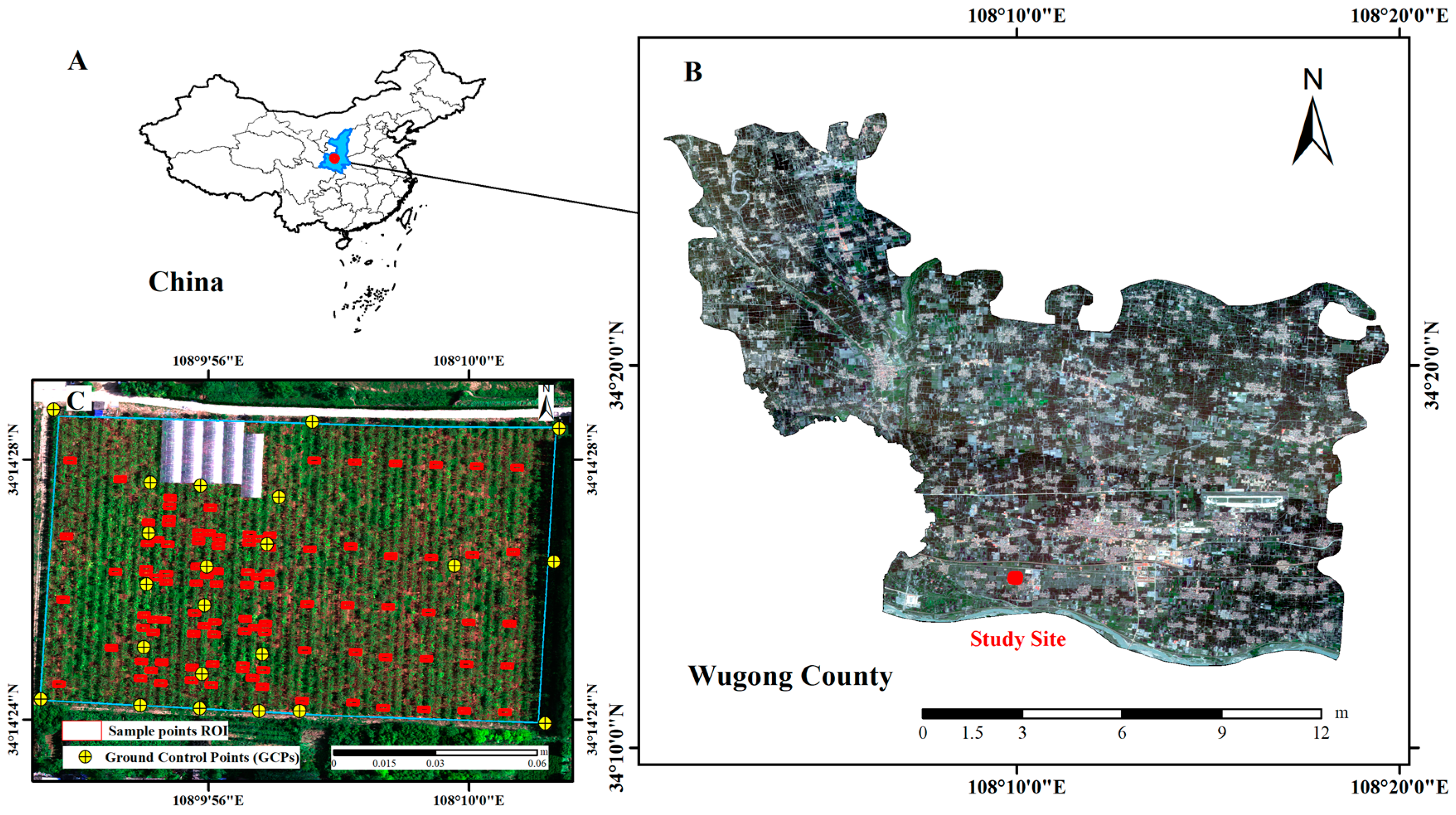
Figure 1. The geographical location of Wugong County and the distribution of sampling sites. (A) Shaanxi’s position in China. (B) Wugong County. (C) Sampling point schematic.
Remotesensing 15 00646 g001
Figure 2. The meteorological data during the sampling period. (Tmin, Tavg, and Tmax are the primary ordinate, and ET, P, and Irrigation are in the secondary ordinate. The intervals of Stage I, Stage II, and Stage III were represented by blue, yellow, and red boxes, respectively, in 2021. Note data from the Weather station in the orchard).
Remotesensing 15 00646 g002
Figure 3. UAV systems and SM sampling in different growth stages. (a) DJI M600pro platform and SM sampling method; (b) Red Edge-MX Dual multispectral camera; (c) Ground control point (GCP); (d) Radiative calibration of calibration board; (e) Stage I—Young fruit stage (20 May 2021); (f) Stage II—Fruit expansion stage (15 August 2021) and (g) Stage III—Fruit maturity stage (9 September 2021).
Remotesensing 15 00646 g003
Figure 4. A workflow diagram of data processing, VIs extraction, and modeling. In (a) Step I, the SVM classification algorithm was used to classify the UAV multi-spectral data to obtain the pure kiwifruit canopy reflectance; in (b) Step II, details of the segmentation process are depicted: starting with mask positioning along planting lines, proceeding with rectangular shape mask extraction; and then in (c) Step III, VIs based on the 2D PLSR-VIP-Rank chart with the measured SM data, were input into RF, SVM, and ELM models, and then obtaining root-zone SM map at three growth stages based on the optimal models.
Remotesensing 15 00646 g004
Figure 5. The violin plots of root SM (SM10, SM20, SM30, SM40, and SM60) values at different kiwifruit key growth stages ((a) Stage I—the young fruit stage, (b) Stage II—the fruit expansion stage and (c) Stage III—the fruit maturity stage).
Remotesensing 15 00646 g005
Figure 6. The rank of VIP between spectral variables and the SM10, SM20, SM30, SM40, and SM60 at three key growth stages ((a) Stage I, (b) Stage II, and (c) Stage III). Note: Redder colors indicate better model performance and higher rankings. Bluer colors indicate worse model performance and lower rankings.
Remotesensing 15 00646 g006
Figure 7. Statistical values of the SVM, RF, and ELM models with a different number of input VIs to estimate (a) SM10, (b) SM20, (c) SM30, (d) SM40, and (e) SM60 at Stage I, II and III. Note: The number of input VIs is 42 (all VIs in this study), 7 (appropriate VIs in Table 3), and 6, 5, 4, 3, 2, 1 (The top 6, 5, 4, 3, 2, 1 VIs in Table 3); the red histogram shows 42 input VIs, and the number of input VIs decreases as the color becomes lighter. The blue values under the line represent the rank of the GPI value (the higher the value, the higher the rank). Best input VIs among all models are marked in blue bold, while the rank of GPI is 1.
Remotesensing 15 00646 g007
Figure 8. Accuracy evaluation (R2, RRMSE, MAE) of optimal root-zone SM model at Stage I, Stage II, and Stage III. Note: the parameters of the optimal root SM models are shown in the bottom table (ML algorithms—RF, SVM, ELM; the number of best input VIs-1 to 7; the input VIs in these best models).
Remotesensing 15 00646 g008
Figure 9. Spatial distribution of different depth SM ((ac) SM10, (df) SM20, (gi) SM30, (jl) SM40, (mo) SM60) at Stage I, Stage II, and Stage III.
Remotesensing 15 00646 g009
Table 1. Technical details of Red-Edge MX Dual camera bands.
BandBand NameSpectral Wavelength (nm)Bandwidth (nm)Function
B1Blue44444428Strong absorption of chlorophyll a and carotenoids.
B2Blue47532
B3Green53153114Strong absorption of chlorophyll and phycoerythrin absorption peak.
B4Green56027Phycoerythrin absorption peak.
B5Red65065016Strong absorption of chlorophyll and phycoerythrin absorption peak.
B6Red66814Strong absorption of chlorophyll, absorption trough of most vegetation.
B7Red-edge70570510Red edge region
B8Red-edge71712
B9Red-edge74074018Strong absorption of chlorophyll
B10NIR84257High reflection of vegetation and the top of red edge region
Table 2. Common spectral indices.
No.IndexFormulationFormula for on Red-Edge MX Dual CameraReference
1NDVI R 840 R 680 R 840 + R 680 B 10 B 6 B 10 + B 6 [36]
2NDRE R 840 R 705 R 840 + R 705 B 10 B 7 B 10 + B 7 [37]
3SCCCI N D R E N D V I /[38]
4RVI R 840 R 680 B 10 B 6 [39]
5NDCI R 762 R 527 R 762 + R 527 B 9 B 3 B 9 + B 3 [40]
6GNDVI R 840 R 705 R 840 + R 705 B 10 B 7 B 10 + B 7 [41]
7OSAVI1 ( 1 + 0.16 ) × ( R 840 R 670 ) R 840 + R 670 + 0.16 ( 1 + 0.16 ) × ( B 10 B 6 ) B 10 + B 6 + 0.16 [42]
8OSAVI2 ( 1 + 0.16 ) × ( R 740 R 670 ) R 740 + R 670 + 0.16 ( 1 + 0.16 ) × ( B 9 B 6 ) B 9 + B 6 + 0.16 (This study)
9VOG1 R 740 R 720 B 9 B 8 [43]
10CARI R 700 R 670 0.2 × ( R 700 + R 670 ) B 7 B 6 0.2 × ( B 7 + B 6 ) [44]
11CARI717 R 717 R 670 0.2 × ( R 717 + R 670 ) B 8 B 6 0.2 × ( B 8 + B 6 ) (This study)
12CARI740 R 740 R 670 0.2 × ( R 740 + R 670 ) B 9 B 6 0.2 × ( B 9 + B 6 ) (This study)
13MTVI1 1.2 × [ 1.2 × ( R 840 + R 550 ) 2.5 × ( R 670 R 550 ) ] 1.2 × [ 1.2 × ( B 10 + B 4 ) 2.5 × ( B 6 B 4 ) ] [45]
14TVI 0.5 × [ 120 × ( R 750 + R 550 ) 2.5 × ( R 670 R 550 ) ] 0.5 × [ 120 × ( B 9 + B 4 ) 2.5 × ( B 6 B 4 ) ] [46]
15DVI R 840 R 680 B 10 B 6 [47]
16RDVI R 840 R 670 R 840 R 670 B 10 B 6 B 10 B 6 [48]
17SPVI 1.48 × ( R 840 R 670 ) 1.2 × | R 530 R 670 | 1.48 × ( B 10 B 6 ) 1.2 × | B 3 B 6 | [44]
18EVI1 2.5 × ( R 840 R 670 ) R 840 6 × R 670 7.5 × R 475 + 1 2.5 × ( B 10 B 6 ) R 840 6 × B 6 7.5 × B 2 + 1 [37]
19EVI2 2.5 × ( R 840 R 670 ) R 840 + 2.4 × R 670 + 1 2.5 × ( B 10 B 6 ) B 10 + 2.4 × B 6 + 1 [49]
20EVI3 2.5 × ( R 840 R 670 ) R 840 2.4 × R 670 + 1 2.5 × ( B 10 B 6 ) B 10 2.4 × B 6 + 1 [50]
21MSAVI1 0.5 × ( 2 × R 840 + 1 [ ( 2 × R 840 + 1 ) 2 8 × R 840 R 670 ] 0.5 ) 0.5 × ( 2 × B 10 + 1 [ ( 2 × B 10 + 1 ) 2 8 × B 10 B 6 ] 0.5 ) [47]
22MSAVI2 0.5 × ( 2 × R 740 + 1 [ ( 2 × R 740 + 1 ) 2 8 × R 740 R 670 ] 0.5 ) 0.5 × ( 2 × B 9 + 1 [ ( 2 × B 9 + 1 ) 2 8 × B 9 B 6 ] 0.5 ) (This study)
23REP1 700 + [ 40 × ( R 668 + R 842 ) × 0.5 R 705 ] R 740 R 705 700 + [ 40 × ( B 6 + B 10 ) × 0.5 B 7 ] B 9 B 7 (This study)
24PRI R 531 R 570 R 531 + R 570 B 3 B 4 B 3 + B 4 [51]
25MTVI2 1.5 × [ 1.2 × ( R 840 R 550 ) 2.5 × ( R 670 R 550 ) ] [ ( 2 × R 840 + 1 ) 2 ( 6 × R 840 5 × R 670 ) 0.5 ] 0.5 1.5 × [ 1.2 × ( B 10 B 4 ) 2.5 × ( B 6 B 4 ) ] [ ( 2 × B 10 + 1 ) 2 ( 6 × B 10 5 × B 6 ) 0.5 ] 0.5 [48]
26TCARI1 3 × [ R 840 R 705 0.2 × ( R 840 R 550 ) × ( R 840 R 705 ) ] 3 × [ B 10 B 7 0.2 × ( B 10 B 4 ) × ( B 10 B 7 ) ] (This study)
27TCARI2 3 × [ R 750 R 705 0.2 × ( R 750 R 550 ) × ( R 750 R 705 ) ] 3 × [ B 9 B 7 0.2 × ( B 9 B 4 ) × ( B 9 B 7 ) ] [52]
28 TCARI 1 OSAVI 1 //[52]
29 TCARI 2 OSAVI 2 //(This study)
30MCARI [ ( R 700 R 670 ) 0.2 × ( R 700 R 550 ) × ( R 700 / R 670 ) ] [ ( B 7 B 6 ) 0.2 × ( B 7 B 4 ) × ( B 7 / B 6 ) ] [53]
31TCAR1 3 × [ ( R 700 R 670 ) 0.2 × ( R 700 R 550 ) × ( R 700 / R 670 ) ] 3 × [ ( B 7 B 6 ) 0.2 × ( B 7 B 4 ) × ( B 7 / B 6 ) ] [53]
32 MCARI OSAVI 1 //[54]
33 MCARI OSAVI 2 //(This study)
34COSRI ( R 527 + R 550 ) × (   R 840 R 670 ) ( R 670 + R 840 ) 2 ( B 2 + B 4 ) × ( B 10 B 6 ) (   B 6 + B 10 ) 2 [55]
35SAVI R 840 R 670 ( 1 + 0.16 ) × ( R 840 + R 670 + 0.16 ) B 10 B 6 ( 1 + 0.16 ) × ( B 10 + B 6 + 0.16 ) [37]
36VARI R 550 R 670 R 550 + R 670 R 527 B 4   B 6 B 4 +   B 6 B 2 [56]
37GLI 2 × R 550 R 527 R 670 2 × R 550 + R 527 + R 670 2 × B 4 B 2 B 6 2 × B 4 + B 2 + B 6 [57]
38IPVI R 840 R 840 + R 670 B 10 B 10 + B 6 [58]
39NNIR R 840 R 840 + R 670 + R 550 B 10 B 10 + B 6 + B 4 [59]
40GCI ( R 840 / R 670 ) 1 ( B 10 / B 6 ) 1 [60]
41RECI ( R 740 / R 670 ) 1 ( B 9 / B 6 ) 1 [60]
42WDRVI 0.12 × R 840 R 670 0.12 × R 840 + R 670 0.12 × B 10 B 6 0.12 × B 10 + B 6 [61]
Note: where Ri is the spectral reflectance of i, which was arbitrarily acquired within the operating range of the remote sensing sensor used in previous research.
Table 3. Appropriate VIs for SM10, SM20, SM30, SM40, and SM60 estimation.
Growth StageResponse VariablesThe Top 7 VIs
1234567
Stage ISM10CARI740MSAVI2MTVI1OSAVI2MTVI2TVIEVI3
SM20MSAVI1RVIRDVIEVI1IPVIOSAVI1VARI
SM30TCARI/OSAVI2OSAVI2TCARI2EVI3SAVINDRENDCI
SM40GLIEVI1TCAR1VARINDVIMSAVI2MCARI
SM60CARI740EVI1MSAVI2MTVI1MTVI2PRIDVI
Stage IISM10TCARI/OSAVI1TCAR1NNIRMTVI2VARIGLIRDVI
SM20EVI3SCCCINDREVOG1NDCIEVI1OSAVI1
SM30EVI2RDVIMTVI2MSAVI2SAVIMSAVI1OSAVI1
SM40TVIEVI3MTVI1MSAVI2DVISPVICARI740
SM60TVICARI740MSAVI2EVI1MTVI1EVI3DVI
Stage IIISM10MTVI1DVISPVIEVI1EVI3CARI740TVI
SM20MTVI1DVISPVIEVI3EVI1TCARI2TVI
SM30MTVI1DVISPVIEVI1EVI3TCARI2TVI
SM40MTVI1DVISPVIEVI3EVI1TCARI2TVI
SM60CARI740MTVI1TVIEVI1DVISPVITCARI2
Table 4. Statistical analysis of root zone SM models based on the number of the best VIs at Stage I.
ModelResponse VariablesNumber of VIs (No. of VIs)Predictive Input VIsR2RRMSEMAEGPIRank
SVMSM105 (12, 22, 13, 8, 25)CARI740, MSAVI2, MTVI1, OSAVI2, MTVI20.790.020.310.073
SM207 (21, 4, 16, 18, 38, 7, 36)MSAVI1, RVI, RDVI, EVI1, IPVI, OSAVI1, VARI 0.700.020.35−0.0610
SM305 (29, 8, 27. 20, 35) TCARI/OSAVI2, OSAVI2, TCARI2, EVI3, SAVI0.780.020.320.064
SM402 (37, 18)GLI, EVI10.700.020.39−0.1012
SM605 (12, 18, 22, 13, 25)CARI740, EVI1, MSAVI2, MTVI1, MTVI20.500.010.27−0.1815
RFSM104 (12, 22, 13, 8)CARI740, MSAVI2, MTVI1, OSAVI20.820.020.200.211
SM203 (21, 4, 16)MSAVI1, RVI, RDVI0.730.020.310.017
SM306 (29, 8, 27. 20, 35, 2) TCARI/OSAVI2, OSAVI2, TCARI2, EVI3, SAVI, NDRE0.720.020.38−0.0811
SM407 (37, 18, 31, 36, 1, 22, 30)GLI, EVI1, TCAR1, VARI, NDVI, MSAVI2, MCARI0.710.020.35−0.059
SM604(12, 18, 22, 13)CARI740, EVI1, MSAVI2, MTVI10.540.010.27−0.1313
ELMSM103 (12, 22, 13)CARI740, MSAVI2, MTVI10.770.020.270.092
SM203 (21, 4, 16)MSAVI1, RVI, RDVI0.730.020.310.025
SM306 (29, 8, 27. 20, 35, 2) TCARI/OSAVI2, OSAVI2, TCARI2, EVI3, SAVI, NDRE0.770.020.340.016
SM403 (37, 18, 31)GLI, EVI1, TCAR10.590.020.20−0.028
SM607 (12, 18, 22, 13, 25, 24,15)CARI740, EVI1, MSAVI2, MTVI1, MTVI2, PRI, DVI0.520.010.28−0.1614
Note: best statistical indicators among all models are highlighted in orange.
Table 5. Statistical analysis of root zone SM models based on the number of the best VIs at Stage II.
ModelResponse VariablesNumber of VIs (No. of VIs)Predictive Input VIsR2RRMSEMAEGPIRank
SVMSM106 (28, 31, 39, 25, 36, 37)TCARI/OSAVI1, TCAR1, NNIR, MTVI2, VARI, GLI0.560.030.46−0.039
SM202 (20, 3)EVI3, SCCCI0.720.020.340.253
SM303 (13,15. 20)MTVI1, DVI, EVI30.690.020.380.196
SM406 (14. 20, 13, 22, 15, 17)TVI, EVI3, MTVI1, MSAVI2, DVI, SPVI0.530.020.53−0.1311
SM602 (14, 12)TVI, CARI7400.300.020.55−0.3814
RFSM106 (28, 31, 39, 25, 36, 37)TCARI/OSAVI1, TCAR1, NNIR, MTVI2, VARI, GLI0.650.020.410.117
SM201 (20)EVI30.760.020.360.282
SM306 (13,15. 20, 17, 19, 16)MTVI1, DVI, EVI3, SPVI, EVI2, RDVI0.710.020.370.225
SM407 (14. 20, 13, 22, 15, 17, 12)TVI, EVI3, MTVI1, MSAVI2, DVI, SPVI, CARI7400.580.020.46−0.018
SM607 (14, 12, 22, 18, 13. 20, 15)TVI, CARI740, MSAVI2, EVI1, MTVI1, EVI3, DVI0.320.030.56−0.3713
ELMSM107 (28, 31, 39, 25, 36, 37, 16)TCARI/OSAVI1, TCAR1, NNIR, MTVI2, VARI, GLI, RDVI0.540.030.45−0.0410
SM207 (20, 3, 2, 9, 5, 18, 7)EVI3, SCCCI, NDRE, VOG1, NDCI, EVI1, OSAVI10.720.020.380.224
SM306 (13,15. 20, 17, 19, 16)MTVI1, DVI, EVI3, SPVI, EVI2, RDVI0.790.020.340.331
SM401 (14)TVI0.520.030.55−0.1712
SM607 (14, 12, 22, 18, 13. 20, 15)TVI, CARI740, MSAVI2, EVI1, MTVI1, EVI3, DVI0.270.030.53−0.4015
Note: best statistical indicators among all models are highlighted in orange.
Table 6. Statistical analysis of root zone SM models based on the number of the best VIs at Stage III.
ModelResponse VariablesNumber of VIs (No. of VIs)Predictive Input VIsR2RRMSEMAEGPIRank
SVMSM101 (13)MTVI10.590.030.490.114
SM204 (13, 15, 17. 20) MTVI1, DVI, SPVI, EVI30.620.040.560.065
SM307 (13, 15, 17, 18. 20, 27, 14)MTVI1, DVI, SPVI, EVI1, EVI3, TCARI2, TVI0.610.030.570.056
SM401 (13)MTVI10.380.040.68−0.3012
SM604(12,13,14,18)CARI740, MTVI1, TVI, EVI10.250.040.62−0.3714
RFSM107 (13, 15, 17, 18. 20, 12, 14)MTVI1, DVI, SPVI, EVI1, EVI3, CARI740, TVI0.670.030.500.183
SM205 (13, 15, 17. 20, 18) MTVI1, DVI, SPVI, EVI3, EVI10.690.030.500.202
SM302 (13, 15)MTVI1, DVI0.730.030.540.211
SM407 (13, 15, 17. 20, 18, 27, 14)MTVI1, DVI, SPVI, EVI3, EVI1, TCARI2, TVI0.490.040.70−0.2210
SM604 (12, 13, 14, 18)CARI740, MTVI1, TVI, EVI10.320.040.67−0.3513
ELMSM104 (13, 15, 17, 18)MTVI1, DVI, SPVI, EVI10.630.040.590.037
SM207 (13, 15, 17. 20, 18, 27,12) MTVI1, DVI, SPVI, EVI3, EVI1, TCARI2, CARI7400.620.050.71−0.109
SM303 (13, 15, 17)MTVI1, DVI, SPVI0.680.040.74−0.078
SM407 (13, 15, 17. 20, 18, 27, 14)MTVI1, DVI, SPVI, EVI3, EVI1, TCARI2, TVI0.560.050.85−0.2911
SM604 (12, 13, 14, 18)CARI740, MTVI1, TVI, EVI10.400.061.07−0.6815
Note: best statistical indicators among all models are highlighted in orange.
Disclaimer/Publisher’s Note: The statements, opinions and data contained in all publications are solely those of the individual author(s) and contributor(s) and not of MDPI and/or the editor(s). MDPI and/or the editor(s) disclaim responsibility for any injury to people or property resulting from any ideas, methods, instructions or products referred to in the content.