Article

Dynamic Detection of Forest Change in Hunan Province Based on Sentinel-2 Images and Deep Learning

1
Key Laboratory of State Forestry and Grassland Administration on Forest Resources Management and Monitoring in Southern Area, Changsha 410004, China
2
College of Forestry, Central South University of Forestry and Technology, Hunan Academy of Forestry, Changsha 410004, China
3
Central South Forest Inventory and Planning Institute of State Forestry Administration, Changsha 410004, China
4
Forestry Research Institute of Guangxi Zhuang Autonomous Region, Nanning 530002, China
*
Author to whom correspondence should be addressed.
Remote Sens. 2023, 15(3), 628; https://doi.org/10.3390/rs15030628
Submission received: 25 October 2022 / Revised: 11 January 2023 / Accepted: 17 January 2023 / Published: 20 January 2023
(This article belongs to the Special Issue Remote Sensing for Mountain Ecosystems)

Abstract

:
Dynamic detection of forest change is the fundamental method of monitoring forest resources and an essential means of preserving the accuracy and timeliness of forest land resource data. This study focuses on a deep learning-based method for dynamic forest change detection using Sentinel-2 satellite data, especially within mountainous areas. First, the performance of various deep learning models (U-Net++, U-Net, LinkNet, DeepLabV3+, and STANet) and various loss functions (CrossEntropyLoss(CELoss), DiceLoss, FocalLoss, and their combinations) are compared on a self-made dataset. Next, the best model and loss function is used to predict the annual forest change in Hunan Province from 2017 to 2021, and the detection results are evaluated in 12 sample areas. Finally, forest changes are detected in Sentinel-2 images for each quarter of 2017–2021. In addition, a dynamic detection map of forest change in Hunan Province from 2017 to 2021 is drawn. The results reveal that the U-Net++ model and the CELoss performed the best on the self-made dataset, with a Precision of 0.795, a Recall of 0.748, and an F1-score of 0.771. The results of annual and quarterly forest change detection were consistent with the changes in the Sentinel-2 images with accurate boundaries. This result demonstrates the high practicality and generalizability of the method used in this paper. This paper achieves a rapid and accurate extraction of multi-temporal Sentinel-2 image forest change areas based on the U-Net++ model, which can be used as a benchmark for future large territorial areas monitoring and management of forest resources.

1. Introduction

Forest resources are essential for global sustainable development, and the rapid transformation of forest environments and the reduction in forest area are major global concerns [1]. Accurate and timely access to forest change information using remote sensing is critical for preserving forest biodiversity and the ecological environment [2]. It is critical to use dynamic forest change detection to complete this task. This paper investigates an efficient method of forest change detection for multi-temporal Sentinel-2 images to map these areas of change more quickly and accurately.
Initially, the surveyors conducted field surveys to gather information on forest resource changes [3]. Due to the lengthy survey cycle and poor timeliness of the survey results, it is difficult for surveyors to keep abreast of the status of forest dynamics changes. To address this question, many forest change studies on integrating spatial and attribute data have emerged since then, yielding various results, including studies on synchronous update strategies and data models.
In recent years, with the continuous development of satellite remote sensing technology [4], remote sensing information collection methods were gradually improved. Remote sensing images are being acquired with greater coverage and precision, and data acquisition cycles are becoming shorter. Consequently, forest change investigation methods have also evolved. For instance, the forest change area is restricted on the remote sensing image. The researchers evaluate and depict the forest change area in the remote sensing image using visual interpretation [5]. This method is faster and more economical than traditional ground surveys. However, a significant portion of the mapping of forest change must be performed by professional researchers. A small amount of change detection data can be well judged by the researcher’s working experience. However, it is easy to miss and misjudge large remote sensing data change detection areas, reducing the work’s quality and efficiency.
To improve the efficiency of mapping areas of forest change, several researchers have developed new detection methods that automatically identify areas of change in remote sensing images [6,7,8]. Many forest change detection methods were proposed and applied to open-source remote sensing data, including MODIS, Landsat, and Sentinel-2 [9]. These detection methods are broadly categorized as image algebra-based methods, image transformation-based methods, and image classification-based methods [10,11]. The methods based on image algebra [12] are those that directly use the differences between different time phases to determine whether a forest has changed. The method based on image transformation [13,14] transforms highly correlated spectral band information into uncorrelated components, thereby effectively reducing data redundancy in the spectral band and enhancing the difference between the changed and unchanged images, thereby allowing for the reliable acquisition of the changed region. The method based on image classification results [15] begins by classifying images from two-time phases. The result of the change detection is then determined by comparing the differences between the image classification results.
As new network structures are proposed and computational costs are reduced, change detection models based on deep learning are also being constructed. A growing number of results demonstrate the widespread implementation and application of deep learning techniques in the field of change detection, as well as the unique advantages of deep learning in image processing. Bousias E. et al. [16] have experimented with two encoder-decoder Convolutional Neural Networks architectures, U-Net and U-Net++ for change detection applications using high-resolution satellite imagery. Their experimental results show that the network trained using the U-Net++ architecture and the data-enhanced network performed best on the test data. Chen H. et al. [17] proposed a spatial-temporal attention-based method applied to the change detection of high-resolution remote sensing image dataset (LEVIR-CD), utilizing a novel spatial-temporal attention-based convolutional neural network (STANet) to improve the accuracy of detection. Lei T. et al. [18] proposed a method for landslide change detection in high-resolution images based on symmetric fully convolutional neural networks. The results demonstrated that this symmetric fully convolutional neural network structure could effectively utilize the spatial multi-scale features of landslide areas and overcome the shortcomings of single-scale ensembles, thereby producing better feature result maps. Sefrin O. et al. [19] utilized a deep learning technique based on Fully Convolutional Networks (FCN) and long short-term memory (LSTM) networks for land cover classification and change detection using multi-temporal and multi-spectral data from the Sentinel-2 satellite, and obtained superior results. Many studies have demonstrated the utility and effectiveness of deep learning-based methods for change detection tasks. Forest change detection, an important branch of this, can also be achieved using deep learning models.
Most of the deep learning-based change detection studies mentioned above are based on high-resolution images. However, the lengthy time required to acquire high-resolution images is not conducive to the rapid detection and dynamic monitoring of forest changes. In addition, there are few studies on forest change detection using deep learning methods. Detecting forest change areas from remote sensing images and mapping them into dynamic detection maps in a timely and accurate manner is a very difficult research-relevant task.
This paper proposes a deep learning-based method for forest change detection on multi-temporal Sentinel-2 remote sensing imagery from 2017 to 2021, as well as mapping the dynamic detection of forest change, based on these findings. The forest change dynamic detection method changes the problems of traditional forest change survey techniques such as long survey periods, overly time-consuming survey process, and inconsistent standards among manual interpretation, and ensures timely and efficient forest change detection work.

2. Materials and Methods

2.1. Study Area

The study area for this paper is Hunan Province, China (Figure 1). Hunan Province is situated in the center of China, between longitudes 108°47′–114°15′E and latitudes 24°38′–30°08′N. The climate of Hunan Province is subtropical monsoon, with hot summers and cold winters. The average annual temperature in Hunan is between 16 and 18 °C, and annual precipitation is between 1200 and 1700 mm [20]. Hunan Province consists of 14 prefecture-level administrative regions, including 13 prefecture-level cities (Changsha, Zhuzhou, Xiangtan, Hengyang, Shaoyang, Yueyang, Changde, Zhangjiajie, Yiyang, Chenzhou, Yongzhou, Huaihua, and Loudi) and one autonomous prefecture (Xiangxi Tujia and Miao Autonomous Prefecture), with a total area of 211,800 square kilometers. The forest vegetation resources belong to the subtropical evergreen broad-leaved forest area. In addition, the main terrain in the study area includes mountains, hills, and plains, which is of great significance for the study of change detection in large areas of mountainous forests.

2.2. Data and Preprocessing

2.2.1. Data Sources

The Sentinel-2 data used in this work were downloaded from the Google Earth Engine (GEE) Open Access Data Centre [21]. Sentinel-2 data provide multispectral images in 13 spectral bands ranging from the visible to the shortwave infrared [22]. It has spatial resolutions of 10m, 20 m, and 60 m, depending on the selected spectral band. In this paper, RGB bands with a spatial resolution of 10 m are used. Four images are downloaded from the GEE platform for each of the study area’s four seasons from 2017 to 2021, for a total of 20 images. The cloud-contained downloaded data are less than 10%, and the areas with cloud higher than 10% are defined as extensive cloud coverage areas. The downloaded Sentinel-2 L1C data products have been processed with radiometric and geometric corrections. The radiometric correction includes correction based on the digital elevation model and atmospheric correction. Due to the vast geographical expanse of our study area, some of our acquired Sentinel-2 remote sensing data contain extensive cloud coverage. In subsequent training and predictions, heavily clouded areas are removed from the images. Table 1 describes the image-specific information used in this study.
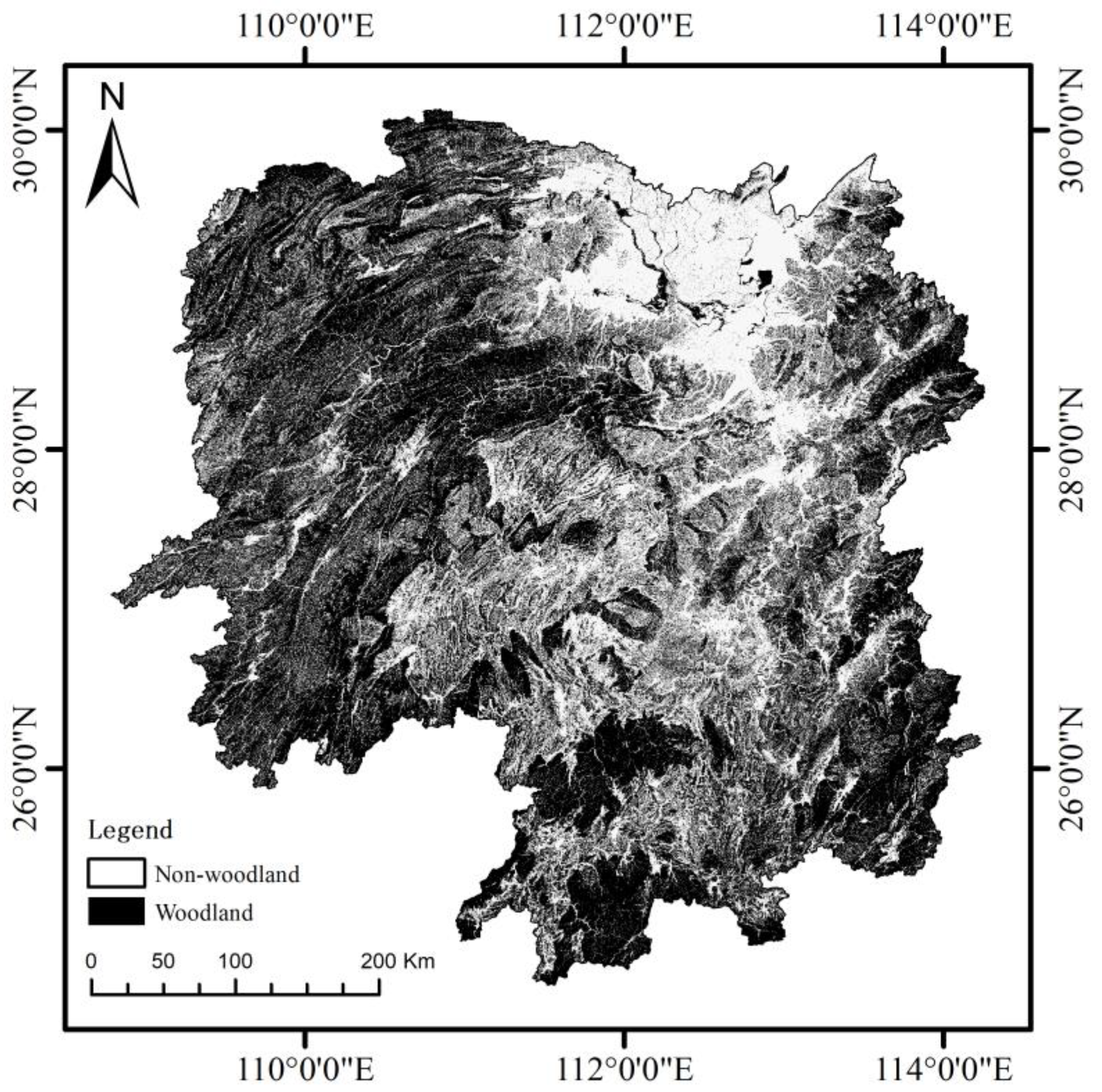
In this paper, only forest change in woodland areas is investigated to avoid detecting areas of forest change in non-woodland areas. The change patches are filtered in non-woodland areas using Woodland Resources Map (Figure 2). As a result, all change patches were from woodland areas.

2.2.2. Dataset

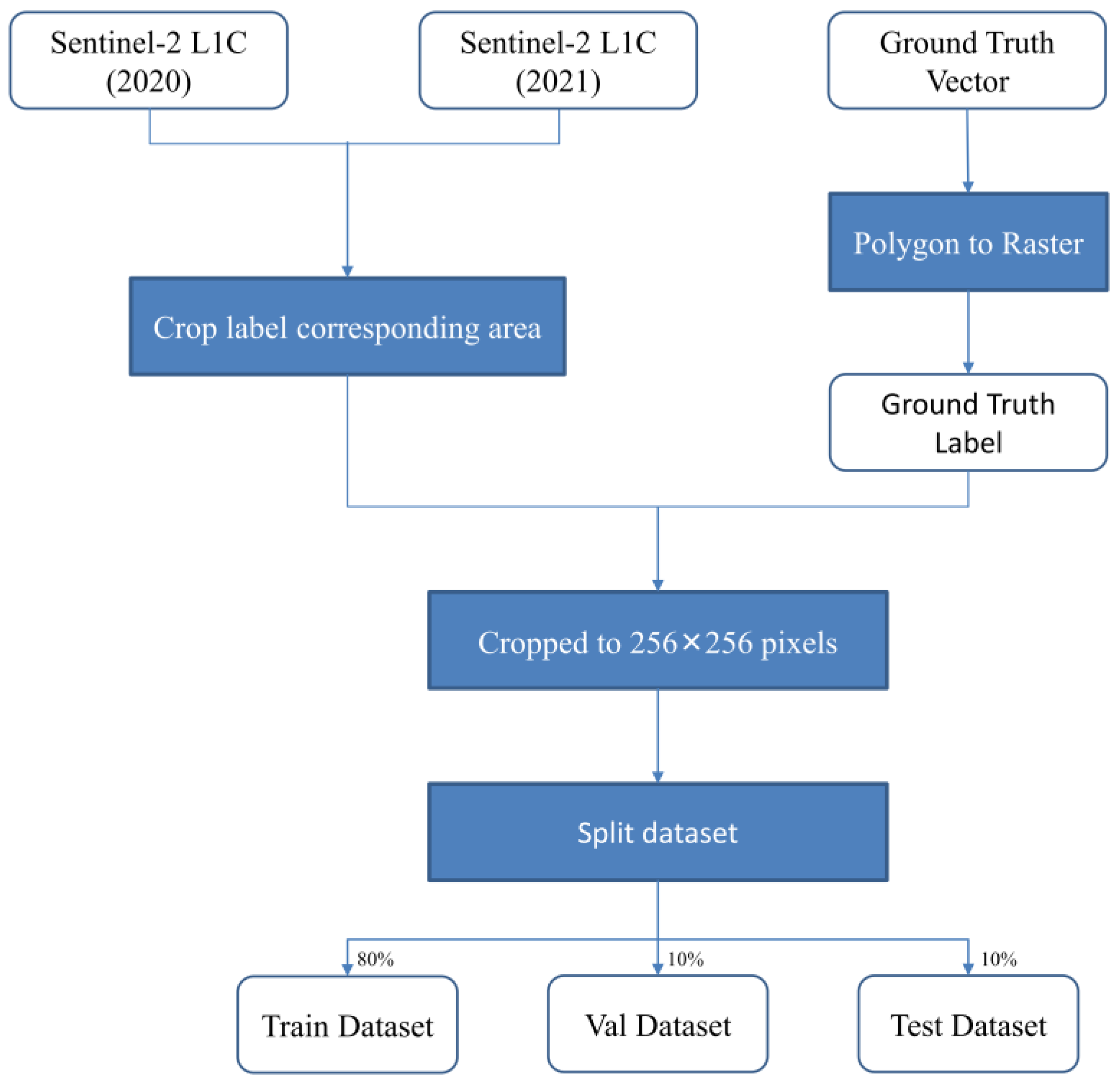
We rely on downloaded Sentinel-2 images and annotate a small number of forest change labels by manual visual interpretation as ground truth vector data. These visual interpretation results were validated by ground surveys. Figure 3 depicts the preprocessing flowchart for the dataset, and the annotation relies on two periods of 2020 and 2021 Sentinel-2 images, respectively. The ground truth vector data were rasterized using ArcMap 10.7 to obtain ground truth labels. The resolution was set to match that of the Sentinel-2 images at 10m. Next, the Sentinel-2 image and ground truth label are cropped to 256 × 256 pixels.
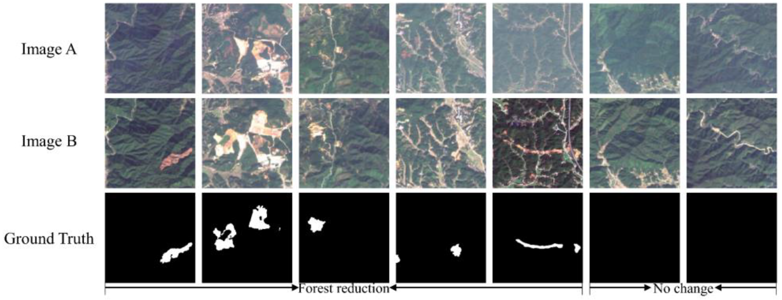
Forest change includes both changes in forest growth and changes in forest reduction. On the one hand, the growth cycle of trees during forest growth is long, with no significant changes in forest growth over the course of a season or even a year, and there is no need for constant monitoring; on the other hand, there are many causes of forest reduction, such as deforestation and clearing, the construction of houses, roads, and other human economic activities [23], which occur in short cycles and require accurate information on their changes. Thus, forest reduction changes are our primary concern. Figure 4 depicts the 256 × 256 pixel images obtained by cropping Sentinel-2 images and ground truth labels, which will be directly used for training and testing deep learning network models. Our dataset contains both positive (areas of forest reduction) and negative samples (no change areas). In addition, the dataset contains a wide variety of forest change image samples. Our dataset contained a total of 1437 image pairs, which were randomly divided into three datasets: the training (train) dataset, the validation (val) dataset, and the test dataset; these three datasets corresponded to an 8:1:1 ratio.

2.2.3. Data Augmentation

This paper employs a variety of image conversion data enhancements, including image panning, horizontal flip, rotation, and brightness adjustment. All data augmentations are designed to improve the generalization of the model and prevent model overfitting.
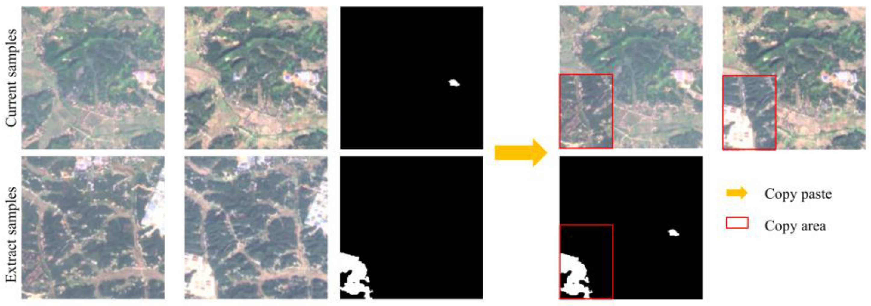
The proportion of positive and negative samples in the dataset is not balanced (Table 2) and only 1.06% of the samples are positive. During the training procedure, the proportion of positive samples is increased by copying and pasting data onto the existing dataset. The specific operation is to randomly extract a sample and paste the changed area into the current sample as an object (Figure 5). In order to better identify the pasted positive samples, we pasted the pixels from the boundary of the change areas as well.

2.3. Change Detection Model

This section details the utilized forest change detection model. In this paper, a U-Net++ [24] deep learning model is used for forest change detection training and prediction. The prediction results of U-Net++ were compared with those of U-Net [25], STANet [17], DeepLabV3+ [26], and LinkNet [27] in order to evaluate the performance of various network models on the self-made dataset and the advantages of the model used in this paper (U-Net++).

2.3.1. The U-Net++ Model

The U-Net++ model structure is derived from the U-Net model, which was originally developed for biological image segmentation tasks and is now widely used for image segmentation and change detection tasks. More importantly, the architecture of U-Net++ is essentially a deeply supervised encoder network in which the encoder and decoder are connected by a series of nested and dense skip roads.
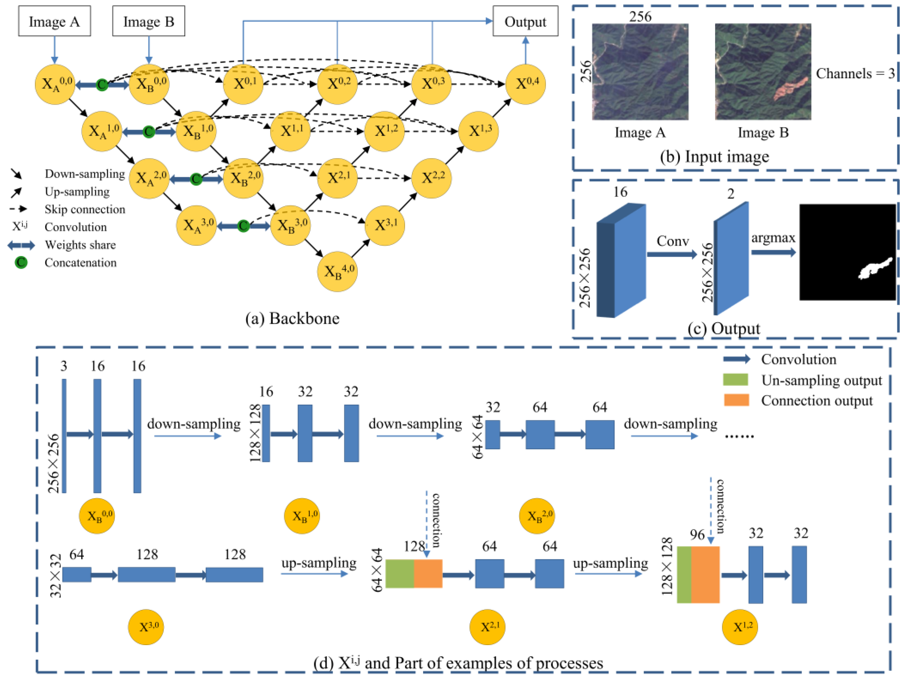
This study adds a two-branch input structure to U-Net++ to ensure that the input of the pre-temporal image and post-temporal image is in the change detection task. U-Net++ is capable of extracting features at various levels and integrating them via a feature overlay. The different levels of features include visible shallow features and abstract deep features, with varying degrees of sensitivity to target objects of different sizes. In practical change detection tasks, the edge information of a large target and a small target can easily be lost in a deep network due to repeated down-sampling and corresponding up-sampling; therefore, shallow features are required to address this issue. U-Net++ is divided into four structures with varying depths, L1, L2, L3, and L4, in order from shallow to deep. In feature extraction, the shallow structure captures simple image features such as borders, colors, etc. The deep structure is able to capture more abstract features within the image due to the larger receptive field and more convolutional operations. The specific network nodes found in L1, L2, L3, and L4, as well as the operations denoted by the arrows in the U-Net++ network structure (Figure 6), are detailed below:
Backbone: In Figure 6a, the L1 of the network structure includes X0,0, X1,0, and X0,1; L2 includes L1 and X2,0, X1,1, and X0,2; L3 includes L2 and X3,0, X2,1, X1,2, and X0,3 and L4 includes all the backbone networks. The output of the network node Xi,j is denoted by xi,j, where i is a down-sampling layer along the encoder index, and j is a convolutional layer along a dense region of the jump path index. The formula for the feature mapping stack denoted by xi,j is as follows:
x i , j = H x i 1 , j , j = 0 H x i , k k = 0 j 1 , U x i + 1 , j 1 , j > 0
where the function H( ) represents the activation function after the convolution operation, U( ) is the up-sampling layer, and [] is the concatenation between the connection of the same layer. As shown in Figure 6a, nodes at layer j = 0 receive only down-sampling inputs from the layer above the encoder; at j > 0 nodes receive (j + 1) inputs, where j inputs are the outputs of the first j nodes in the Concatenation same skip pathway. The last input is the up-sampling output from the lower skip path or encoder (when j = 1).
Down-sampling: The purpose of down-sampling is to increase the image’s robustness against small perturbations. In this paper, the encoder employs the Efficientnet-b0 algorithm for down-sampling. Down-sampling halves the image’s height and width while doubling the number of channels, compressing the 2 × 2 pixel blocks into a single pixel, and averaging the values of four pixels.
Up-sampling: The function of up-sampling is to decode the abstract features to the same size as the original image dimensions to obtain the segmentation result. This is accomplished by doubling the image’s height and width and halving the number of channels, effectively replacing each pixel with a 2 × 2 block of identically valued pixels.
Skip connection: As indicated by [] in Equation (1), it is a connection with dense nesting on the skip path.
Convolution (Conv): Each convolutional node Xi,j is made up of three convolutional layers (Figure 6d), each with a convolutional kernel of 3 × 3. The number of filters in each convolutional node is also different due to the constant down-sampling and up-sampling. The number of filters in terms of Fn is given by:
F n = 16 ( i + 1 ) , i 0 , 1 , 2 , 3 , 4
Concatenation: Images A and B are merged so that the final number of channels is the sum of A and B, with the same width and height.
The experimental environment in this paper is based on the Pytorch framework and the Python language. It was developed using Windows 10 and an Nvidia RTX3080ti GPU with 12GB of video memory and Compute Unified Device Architecture version 11.0 for training. The server used for deep learning is equipped with a 3.79 GHz Intel(R) Core(TM) i7-10700KF processor, 32 GB of RAM, and 4 TB of storage space.

2.3.2. Loss Function

The standard cross-entropy function CrossEntropyLoss function [28] (CELoss) is more helpful when solving the sample imbalance (Table 2), so the CELoss function is chosen as the loss function in this paper. CELoss combines the activation function LogSoftmax and the loss function NLLLoss:
L o g S o f t m a x ( x ) = log e e x j i = 1 n e x i ,
N L L L o s s = 1   N i = 1 N y i ( L o g S o f t m a x ) ,
C E L o s s = L o g S o f t m a x + N L L L o s s ,
LogSoftmax is the logarithm of the softmax function. The output of the softmax function is a vector between [0, 1], so the LogSoftmax function has a value range of (−∞, 0]. The NLLLoss function is obtained by averaging the product of yi and the output of the LogSoftmax function and inverting it. CELoss is the value of the sum of LogSoftmax and NLLLoss.
We also used DiceLoss [29], FocalLoss [30], a combination of CELoss and FocalLoss, a combination of CELoss and DiceLoss, and a combination of DiceLoss and FocalLoss (with a weight ratio of 1:1 when the two loss functions were combined) in the U-Net++ change detection model for the test dataset and compared their predictions.

2.3.3. Accuracy Evaluation Metrics

In this paper, the statistical unit for calculating accuracy evaluation metrics is a single image element. The following accuracy evaluation metrics that are widely used in the change detection field are calculated: Precision, Recall, and F1-score are displayed in Equations (6)–(8). F1-score is the harmonic mean of Precision and Recall, which more accurately reflects the model’s performance on unbalanced datasets [31].
P r e c i s i o n = T P T P + F P ,
R e c a l l = T P T P + F N ,
F 1 - s c o r e = 2 × P r e c i s i o n × R e c a l l P r e c i s i o n + R e c a l l ,
In these equations, TP is the area of pixels where positive samples are correctly predicted, FP is the area of pixels incorrectly predicted as positive samples, and FN is the area of pixels where positive samples are missed.

2.4. Dynamic Detection of Forest Change

We quantify the extent and rate of forest change (reduction) from results on a larger regional scale and understand the specific periods of forest change for dynamic detection. Incorporating elements of temporal change analysis into the process of detecting forest change over large areas is crucial. Annual forest change areas and quarterly forest change areas in Hunan Province were predicted and analyzed for the years 2017 to 2021 using the optimal model identified in the previous section and the loss function.

2.4.1. Annual Forest Change Detection

To validate the methods used in this paper for detecting forest change and analyzing the specifics of forest change from year to year, the forest changes are predicted in Hunan Province from 2017 to 2021. The current year’s winter Sentinel-2 image is used as the post-temporal image, while the previous year’s winter Sentinel-2 image is used as the pre-temporal image (the 2017 pre-temporal image is the 2017 spring Sentinel-2 image) to input into the forest change detection network in order to obtain forest change detection results for each year.
Then, 12 sample areas were randomly selected in Hunan Province (each sample area is 1224 km2, Figure 1b). These areas are distributed across locations in Hunan Province. The results of forest change detection are compared to areas of actual ground change and evaluated for each year and sample area. In this paper, the results of change detection are presented in the form of graphs and tables.

2.4.2. Quarterly Forest Change Detection

To further analyze the precise timing and magnitude of forest change in the study area, we fed two periods of Sentinel-2 data, separated by one quarter, into the forest change detection network and predicted changes in forest reduction for each quarter between 2017 and 2021 using the forest change detection model.
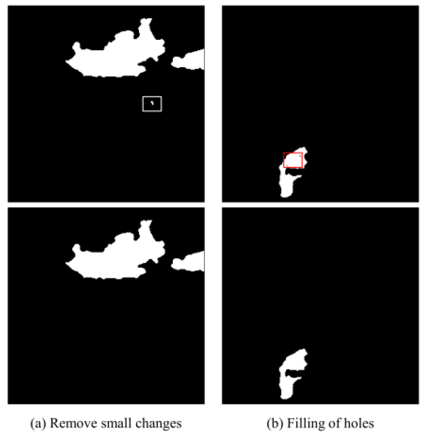
First, to improve the accuracy of our forest change detection method, we removed changes in non-woodland areas using the Woodland Resources Map of the study area mentioned in Section 2.2.1 (Table 1). Second, we utilized a forest change detection model to forecast quarterly forest change in the study area. After verifying the results map for each period, the results map is post-processed. To refine the final detection results, the threshold method and morphological post-processing [32] were used to remove very small area patches, small gaps, and the presence of holes within the area of change from the forest change detection results images (Figure 7). Eventually, we combined the results of the processed forest change area maps for each quarter into a single map and used different colors to indicate the different periods’ change patches. Each area of forest change will be labeled at a specific time.

3. Results

3.1. Change Detection Results in the Dataset

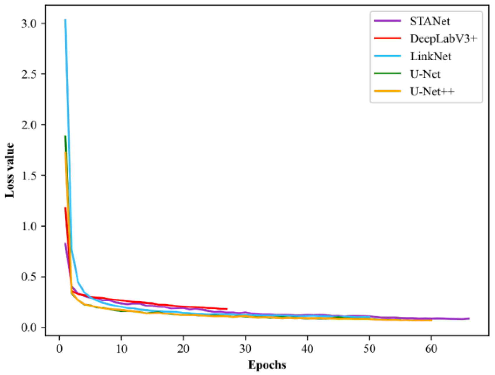
During model training, the test dataset does not contribute to the construction of the model (training and validation and tuning of hyperparameters). The maximum training epoch for all models was set to 100; an early stop was added to the training process to prevent overfitting of the models. The early stop is the termination of the model training when the model has not been updated for a long time. Figure 8 demonstrates the specific trend of Loss values for each model during the training process, and it can be seen that the specific Early Stop time is different for each model.
The performance of U-Net++ and other models is evaluated on the test dataset. The comparison results show that the U-Net++ model used in this paper is optimal in all accuracy evaluation metrics in the test dataset, with a Precision of 0.7954, a Recall of 0.7478, and an F1-score of 0.7709 (Table 3). U-Net++ is superior to other change detection models (U-Net, LinkNet, DeepLabV3+, STANet) in terms of precision and detection rate. The F1-score represents the harmonic mean of Precision and Recall. A greater value indicates greater model stability. Regarding the training speed of the models, the batch size of each forest change detection model is set to the maximum memory can afford, and the mean time in Table 3 represents the average training time per epoch. U-Net++ spent 0.89 minutes per epoch, which is only 0.07 min more than U-Net, which spent the least time per epoch. This paper concludes that U-Net++ outperforms other forest change detection models (U-Net, LinkNet, DeepLabV3+, and STANet) in terms of accuracy, balance, and other comprehensive performance on a self-made dataset.
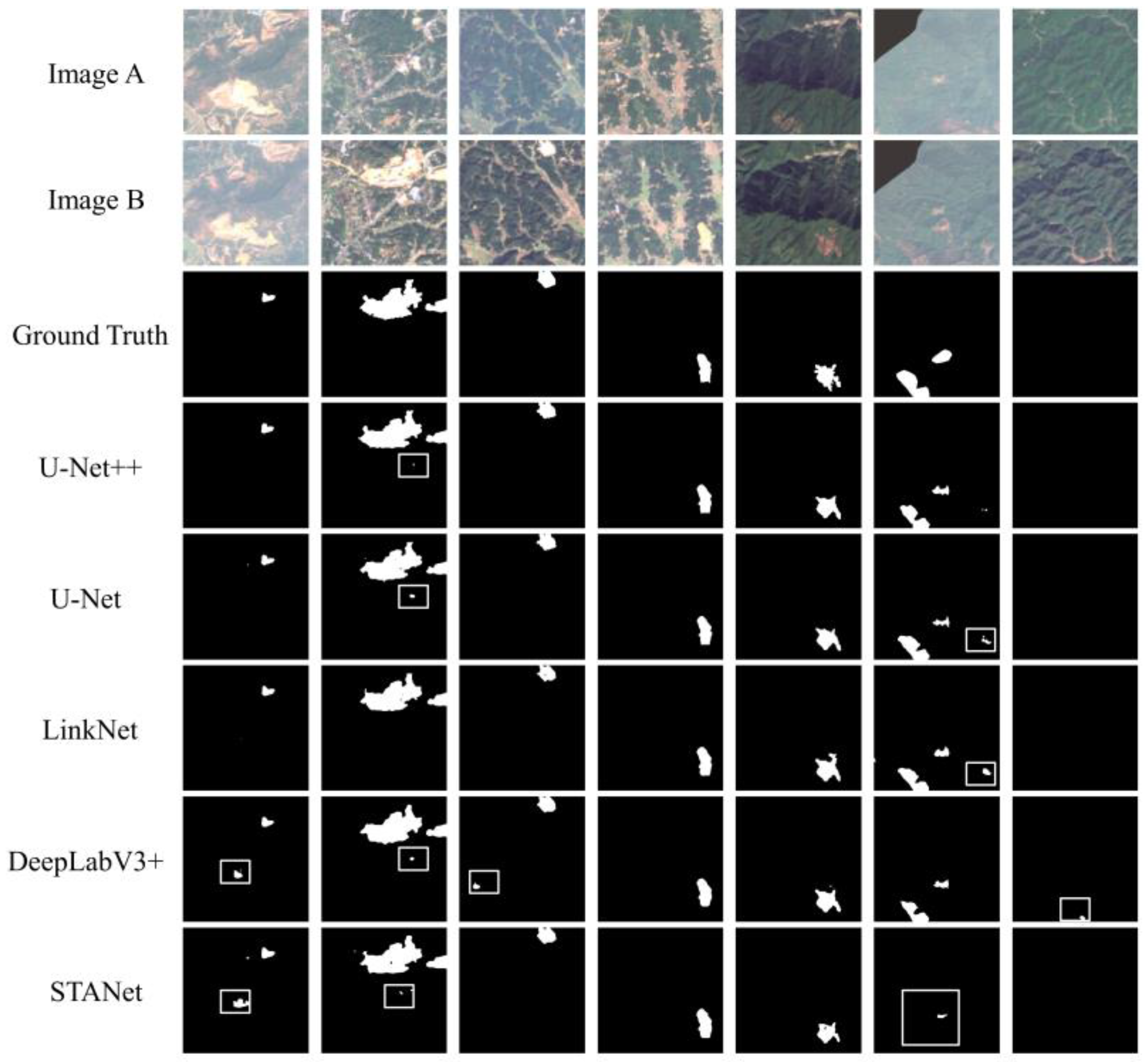
A comparison of the spatial mapping results for each change detection model for the same loss function condition with the labels of the test dataset is shown in Figure 9. The predictions of the U-Net++ model are most similar in space to the reference labels. Moreover, it is more refined in terms of boundary drawing, which is due to the fact that U-Net++ integrates features at different levels by capturing them in a feature overlay, allowing it to choose a network structure of different depths depending on the complexity of the current dataset.
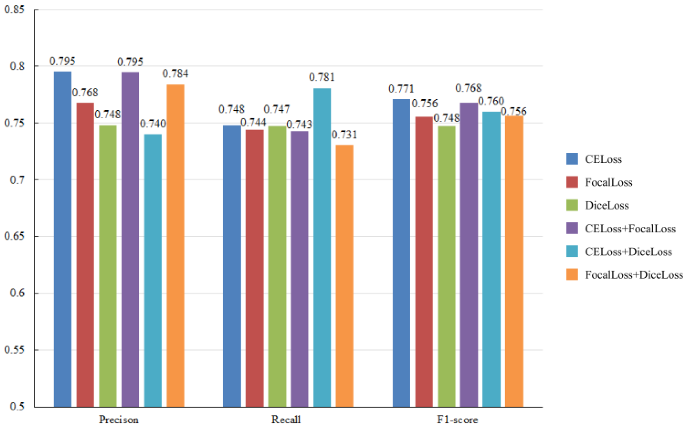
In addition to comparing the prediction results of various deep learning models, some experiments are conducted to compare the U-Net++ change detection model under various loss function combinations. The experimental results are shown in Figure 10. The U-Net++ model, when paired with CELoss, has a test Precision of 0.795, Recall of 0.748, and F1-score of 0.771, with the best overall performance among all combinations of loss functions. CELoss has the highest Precision and detects changes with the least pseudo changes compared to DiceLoss, FocalLoss, and other combinations of loss functions. The CELoss function with the best overall performance is selected for subsequent annual and quarterly forest change detection over large areas.

3.2. Annual Forest Change Detection Results

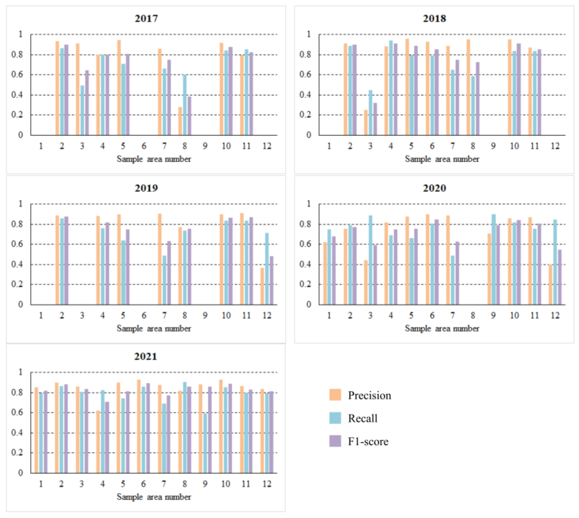
Figure 11 depicts the evaluation of the accuracy of the selected 12 sample areas for the annual change detection results from 2017 to 2021 during the analysis of the quantitative results. The F1-score of 0.8 was achieved in all sample areas except those numbered 3, 7 and 8 in 2017, 2018 and 2020, those numbered 7 and 8 in 2019, those numbered 1, 3, 6 and 9 in 2019 and those not involved in the assessment. For the sample areas where the F1-score was not high, a review of the detection results with two periods of Sentinel-2 images revealed that the main cause of the misdetection was a small number of clouds being detected as areas of forest reduction.
In the overall assessment of accuracy for all sample areas, the F1-score was above 0.75 for each year and above 0.8 in 2018 and 2021. The year with the lowest accuracy metric was 2020 with a Precision of 0.749, Recall of 0.759, and F1-score of 0.754, and the year with the highest accuracy metric was 2021 with a Precision of 0.839, Recall of 0.819, and F1-score of 0.829 (Table 4). These figures are in general agreement with the accuracy tested in the dataset. The annual forest change detection prediction results demonstrate that the U-Net++ model utilized in this paper achieves excellent results in large-area image detection and stable performance in detecting images from different years. In addition, it takes only 40 minutes to predict the results of forest change detection in the whole Hunan Province. This method provides the foundation for subsequent dynamic forest change detection tasks and important guidance for the annual forest change survey.

3.3. Quarterly Forest Change Dynamics Detection and Mapping

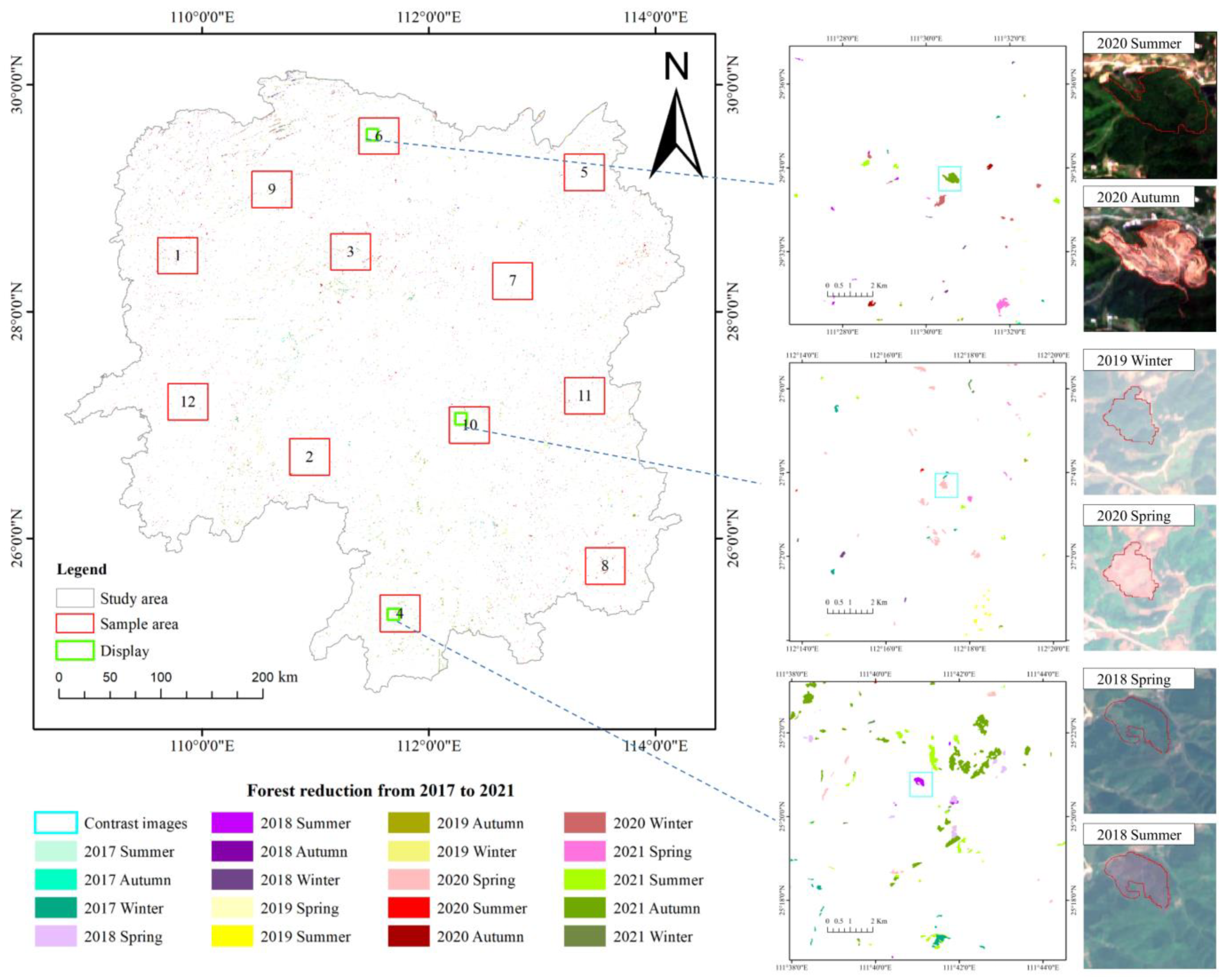
The U-Net++ model and CELoss loss function are utilized to forecast forest change for every quarter between 2017 and 2021. Following the mapping procedure outlined in Section 2.4.2, a regional map of quarterly forest change in Hunan Province from 2017 to 2021 is created (Figure 12). Comparing the quarterly forest reduction results map of Hunan Province with the Sentinel-2 time series images from 2017 to 2021 reveals that the areas extracted by the forest change detection model correspond precisely to the actual image boundaries.
Analyzing the detection in the sample areas with the Sentinel-2 images reveals that their quarterly forest change detection is consistent with the annual detection in Section 3.2. In the analysis of the vector map of change detection results, the forest change area in each quarter of 2017 was smaller than in other years. After comparing the 2017 images to their corresponding Sentinel-2 images, it was found that all four 2017 images contained large areas of missing imagery (due to excessive cloudiness), which interfered with the forest change detection task.

4. Discussion

In this paper, the performance of a deep learning-based method (U-Net++) is evaluated using a custom dataset and province-wide Sentinel-2 image forest change detection. Specifically, a comprehensive method for monitoring forest change using Sentinel-2 images for dynamic detection and mapping of forest change in large territorial areas was developed. Importantly, our method can be trained using samples collected at a specific time in a region, with good transferability to new time periods and images from different regions.

4.1. Performance Evaluation of Forest Change Detection Models

As shown in Table 3, the U-Net++ model produced the highest Precision, Recall, and F1-score. This result indicates that the U-Net++ model is better adapted to the dataset produced by Sentinel-2 imagery after training on this dataset. No additional training images from its year and region were added to the dataset beyond those from the specific temporal and spatial region mentioned in Section 2.2.2 (Figure 3), as indicated by the smaller Precision and Recall for the STANet. In the model comparison experiments, the F1-score of DeepLabV3+ was 2.72% lower than that of U-Net++, but it took more time to train per epoch (12.35 min per epoch). In terms of image mapping results, U-Net is inferior to U-Net++, and its boundaries are coarser (Figure 9). This result conforms to the U-Net++ characteristics described in Section 2.3.1. Consequently, the overall performance of the U-Net++ model is superior to that of other change detection models based on the test results of the self-made dataset presented in this paper.
In the following, the comparison of accuracy in the U-Net++ forest change detection model is discussed using different combinations of loss functions (Figure 10). Using the CELoss function, the model’s Precision and F1-score are the highest among all combinations of loss functions, while its Recall is the second highest (0.047 lower than the highest value). Therefore, the overall performance of the model when utilizing this loss function is the best among all possible combinations of loss functions. This result demonstrates that the best detection results are obtained when the CELoss function is used as a loss function on a self-made dataset with positive and negative sample imbalance.

4.2. Performance Evaluation of Annual Forest Change Detection

In Sentinel-2 images without clouds, the experimental results from Section 3.2 (Figure 11, Table 4) demonstrate that our model is effective at detecting forest changes over large areas. This result does not differ significantly from the F1-score obtained from predictions in the self-made dataset, with higher detection accuracy in some years than predictions in the test dataset (2017–2019,2021). The detection results of the model are compared with the labels obtained by manual visual interpretation.The results obtained from the model detection were found to be more accurate and refined in drawing the boundary of the changed patch.
In addition, the detection accuracy of this study is good in both mountainous areas and plains. From Figure 1, it can be concluded that the sample areas numbered 5, 6, 7, 10, and 11 are in the plain area and the other sample areas are in the mountainous forest. According to the results of Figure 11, the accuracy difference between them is not significant.

4.3. The Advantages of Quarterly Forest Change Dynamics Detection

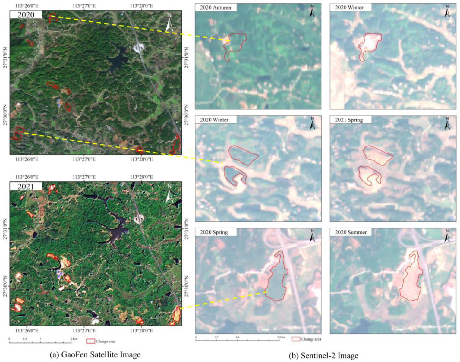
In Section 3.3, we project quarterly forest changes for the period 2017–2021. Based on them, the results of the quarterly dynamic detection of forest change from 2017 to 2021 are mapped (Figure 12). In the process of detecting forest changes at short intervals, we are able to obtain the precise time of each change patch and analyze the causes of its change in order to achieve timely detection and real-time monitoring. This is essential for monitoring the renewal status of forest resources and carrying out management [33]. As illustrated in Figure 13, forest change patches are detected on GaoFen satellite images for 2020–2021. However, we only know that these changes occurred during 2020–2021; we were unable to determine the exact quarter in which they occurred. Therefore, the precise timing of the changes can be determined using the method described in this paper to obtain quarterly forest change dynamics detection results based on the more frequently updated Sentinel-2 images.

4.4. Outlook

Our proposed method for dynamic detection of forest change can accurately identify forest changes in areas without clouds, but cannot obtain information on changes in areas with large cloud cover, which leads to incomplete final prediction results and mapping results. Therefore, we will address this aspect in future studies by selecting median synthesis methods and Sentinel-1 images to predict forest changes. Multiple predictions will be used for cross-validation, supplementing them for areas with high cloud cover, to achieve multiple source detection and more comprehensive dynamic detection of forest change.

5. Conclusions

Forest change detection is crucial for many applications and research fields, such as forest resource evaluation and management. For example, in the investigation of forest land resource change, the quarterly and monthly change information of forest land resources can be updated through the method of forest dynamic change detection and significantly improve the timeliness of forest resource monitoring. To solve the problem of forest change dynamics detection, Sentinel-2 data are used in conjunction with a deep learning method based on the U-Net++ model to complete the forest change detection task for each quarter from 2017 to 2021, and then the results of forest change dynamic detection are plotted.
First, several deep learning models are trained and evaluated on self-made datasets, with U-Net++ used in this paper exhibiting the best overall performance. On this basis, additional comparison experiments with different combinations of loss functions are designed. As expected, the loss function with the most prominent effect was CELoss. Comparative experiments with different deep learning models and loss functions provide the basis for subsequent dynamic detection of forest change. Second, the U-Net++ model and CELoss are employed to predict the Sentinel-2 images for each year from 2017 to 2021 and to evaluate the detection results for the 12 sample areas. The results demonstrate that the method utilized in this paper is highly accurate and applicable for detecting large-area forest changes in Sentinel-2 images. Finally, the results of the quarterly dynamic detection of forest changes from 2017 to 2021 were mapped.
The results of this paper can be used as a reference for dynamic detection of forest change in medium resolution and short interval remote sensing images, and they are feasible for practical forest change detection tasks. Especially, the detection of forest change in large areas is of great practical value. According to the results of this paper, the annual and quarterly forest change detection results of the region are derived, which ensure the timeliness of forest change detection and enable the monitoring of forest resources in real-time. Based on the rapid updating of remote sensing images, an integrated forest resource monitoring technology integrating remote sensing technology and deep learning technology is established, and theoretical research is applied to actual production.

Author Contributions

J.X. wrote the manuscript and designed the comparative experiments; D.M. supervised the study and revised the manuscript; Y.X. supervised the study and provided data; W.W. and E.Y. revised the manuscript and gave comments and suggestions to the manuscript; J.J. assisted J.X. in designing the architecture and conducting experiments. All authors have read and agreed to the published version of the manuscript.

Funding

This research was funded by the National Natural Science Foundation of China under Grant 32071682 and Grant 31901311; In part by the Project of Central South Inventory and Planning Institute of State Forestry and Grassland Administration “Research on key technologies of large-scale deployable remote sensing-based intelligent forest change monitoring system” Science and Technology Innovation Plan Project of Hunan Provincial Forestry Department under Grant XLK202108-8 and funded by College Students’ Innovative Entrepreneurial Training Plan Program under Grant QL20220178.

Data Availability Statement

Not applicable.

Conflicts of Interest

The authors declare no conflict of interest.

References

  1. Desclée, B.; Bogaert, P.; Defourny, P. Forest change detection by statistical object-based method. Remote Sens. Environ. 2006, 102, 1–11. [Google Scholar] [CrossRef]
  2. Lechner, A.M.; Foody, G.M.; Boyd, D.S. Applications in Remote Sensing to Forest Ecology and Management. One Earth 2020, 2, 405–412. [Google Scholar] [CrossRef]
  3. Carney, J.; Gillespie, T.W.; Rosomoff, R. Assessing forest change in a priority West African mangrove ecosystem: 1986–2010. Geoforum 2014, 53, 126–135. [Google Scholar] [CrossRef]
  4. Boyd, D.S.; Danson, F.M. Satellite remote sensing of forest resources: Three decades of research development. Prog. Phys. Geogr. Earth Environ. 2005, 29, 1–26. [Google Scholar] [CrossRef]
  5. Panigrahy, R.K.; Kale, M.P.; Dutta, U.; Mishra, A.; Banerjee, B.; Singh, S. Forest cover change detection of Western Ghats of Maharashtra using satellite remote sensing based visual interpretation technique. Curr. Sci. 2010, 98, 657–664. Available online: https://www.jstor.org/stable/24111818 (accessed on 18 January 2022).
  6. Chen, J.; Gong, P.; He, C.; Pu, R.; Shi, P. Land-use/land-cover change detection using improved change-vector analysis. Photogramm. Eng. Remote Sens. 2003, 69, 369–379. [Google Scholar] [CrossRef] [Green Version]
  7. Asokan, A.; Anitha, J. Change detection techniques for remote sensing applications: A survey. Earth Sci. Inform. 2019, 12, 143–160. [Google Scholar] [CrossRef]
  8. Chen, X.; Chen, J.; Shi, Y.; Yamaguchi, Y. An automated approach for updating land cover maps based on integrated change detection and classification methods. ISPRS J. Photogramm. Remote Sens. 2012, 71, 86–95. [Google Scholar] [CrossRef]
  9. Zhu, Z. Change detection using landsat time series: A review of frequencies, preprocessing, algorithms, and applications. ISPRS J. Photogramm. Remote Sens. 2017, 130, 370–384. [Google Scholar] [CrossRef]
  10. Singh, A. Review Article Digital change detection techniques using remotely-sensed data. Int. J. Remote Sens. 1989, 10, 989–1003. [Google Scholar] [CrossRef] [Green Version]
  11. Lu, D.; Mausel, P.; Brondízio, E.; Moran, E. Change detection techniques. Int. J. Remote Sens. 2004, 25, 2365–2401. [Google Scholar] [CrossRef]
  12. Fan, H.; Fu, X.; Zhang, Z.; Wu, Q. Phenology-Based Vegetation Index Differencing for Mapping of Rubber Plantations Using Landsat OLI Data. Remote Sens. 2015, 7, 6041–6058. [Google Scholar] [CrossRef] [Green Version]
  13. Huesca, M.; García, M.; Roth, K.L.; Casas, A.; Ustin, S.L. Canopy structural attributes derived from AVIRIS imaging spectroscopy data in a mixed broadleaf/conifer forest. Remote Sens. Environ. 2016, 182, 208–226. [Google Scholar] [CrossRef] [Green Version]
  14. Jin, S.; Sader, S.A. Comparison of time series tasseled cap wetness and the normalized difference moisture index in detecting forest disturbances. Remote Sens. Environ. 2005, 94, 364–372. [Google Scholar] [CrossRef]
  15. Xie, G.; Niculescu, S. Mapping and Monitoring of Land Cover/Land Use (LCLU) Changes in the Crozon Peninsula (Brittany, France) from 2007 to 2018 by Machine Learning Algorithms (Support Vector Machine, Random Forest, and Convolutional Neural Network) and by Post-classification Comparison (PCC). Remote Sens. 2021, 13, 3899. [Google Scholar] [CrossRef]
  16. Alexakis, E.B.; Armenakis, C. Evaluation of UNet and UNet++ architectures in high resolution image change detection applications. Int. Arch. Photogramm. Remote Sens. Spat. Inf. Sci. 2020, 43, 1507–1514. [Google Scholar] [CrossRef]
  17. Chen, H.; Shi, Z. A spatial-temporal attention-based method and a new dataset for remote sensing image change detection. Remote Sens. 2020, 12, 1662. [Google Scholar] [CrossRef]
  18. Lei, T.; Zhang, Q.; Xue, D.; Chen, T.; Meng, H.; Nandi, A.K. End-to-end Change Detection Using a Symmetric Fully Convolutional Network for Landslide Mapping. In Proceedings of the ICASSP 2019—2019 IEEE International Conference on Acoustics, Speech and Signal Processing (ICASSP), Brighton, UK, 12–17 May 2019; pp. 3027–3031. [Google Scholar]
  19. Sefrin, O.; Riese, F.M.; Keller, S. Deep learning for land cover change detection. Remote Sens. 2020, 13, 78. [Google Scholar] [CrossRef]
  20. Hu, Y.; Xu, X.; Wu, F.; Sun, Z.; Xia, H.; Meng, Q.; Huang, W.; Zhou, H.; Gao, J.; Li, W. Estimating forest stock volume in Hunan Province, China, by integrating in situ plot data, Sentinel-2 images, and linear and machine learning regression models. Remote Sens. 2020, 12, 186. [Google Scholar] [CrossRef] [Green Version]
  21. Mutanga, O.; Kumar, L. Google earth engine applications. Remote Sens. 2019, 11, 591. [Google Scholar] [CrossRef] [Green Version]
  22. Drusch, M.; Del Bello, U.; Carlier, S.; Colin, O.; Fernandez, V.; Gascon, F.; Hoersch, B.; Isola, C.; Laberinti, P.; Martimort, P.; et al. Sentinel-2: ESA’s Optical High-Resolution Mission for GMES Operational Services. Remote Sens. Environ. 2012, 120, 25–36. [Google Scholar] [CrossRef]
  23. Zhu, J.-J.; Li, F.-Q. Forest degradation/decline: Research and practice. Ying Yong Sheng Tai Xue Bao J. Appl. Ecol. 2007, 18, 1601–1609. Available online: https://europepmc.org/abstract/MED/17886658 (accessed on 18 January 2022).
  24. Zhou, Z.; Rahman Siddiquee, M.M.; Tajbakhsh, N.; Liang, J. UNet++: A Nested U-Net Architecture for Medical Image Segmentation. In Deep Learning in Medical Image Analysis and Multimodal Learning for Clinical Decision Support; Springer: Cham, Switzerland, 2018; pp. 3–11. [Google Scholar]
  25. Ronneberger, O.; Fischer, P.; Brox, T. U-Net: Convolutional Networks for Biomedical Image Segmentation. In Proceedings of the Medical Image Computing and Computer-Assisted Intervention—MICCAI 2015, Munich, Germany, 5–9 October 2015; Springer: Cham, Switzerland, 2015; pp. 234–241. [Google Scholar]
  26. Chen, L.-C.; Zhu, Y.; Papandreou, G.; Schroff, F.; Adam, H. Encoder-decoder with atrous separable convolution for semantic image segmentation. In Proceedings of the European Conference on Computer Vision (ECCV), Munich, Germany, 8–14 September 2018; pp. 801–818. [Google Scholar]
  27. Chaurasia, A.; Culurciello, E. LinkNet: Exploiting encoder representations for efficient semantic segmentation. In Proceedings of the 2017 IEEE Visual Communications and Image Processing (VCIP), St. Petersburg, FL, USA, 10–13 December 2017; pp. 1–4. [Google Scholar]
  28. Zhang, Z.; Sabuncu, M. Generalized cross entropy loss for training deep neural networks with noisy labels. In Proceedings of the 32nd International Conference on Neural Information Processing Systems, Montreal, QC, Canada, 3–8 December 2018; pp. 8792–8802. [Google Scholar]
  29. Milletari, F.; Navab, N.; Ahmadi, S.A. V-Net: Fully Convolutional Neural Networks for Volumetric Medical Image Segmentation. In Proceedings of the 2016 Fourth International Conference on 3D Vision (3DV), Stanford, CA, USA, 25–28 October 2016; pp. 565–571. [Google Scholar]
  30. Lin, T.-Y.; Goyal, P.; Girshick, R.; He, K.; Dollar, P. Focal Loss for Dense Object Detection. In Proceedings of the 2017 IEEE International Conference on Computer Vision (ICCV), Venice, Italy, 22–29 October 2017; pp. 2999–3007. [Google Scholar]
  31. Hand, D.; Christen, P. A note on using the F-measure for evaluating record linkage algorithms. Stat. Comput. 2018, 28, 539–547. [Google Scholar] [CrossRef] [Green Version]
  32. Haralick, R.M.; Sternberg, S.R.; Zhuang, X. Image Analysis Using Mathematical Morphology. IEEE Trans. Pattern Anal. Mach. Intell. 1987, 4, 532–550. [Google Scholar] [CrossRef]
  33. Mani, J.K.; Varghese, A.O. Remote Sensing and GIS in Agriculture and Forest Resource Monitoring. In Geospatial Technologies in Land Resources Mapping, Monitoring and Management; Reddy, G.P.O., Singh, S.K., Eds.; Springer International Publishing: Cham, Switzerland, 2018; pp. 377–400. [Google Scholar]
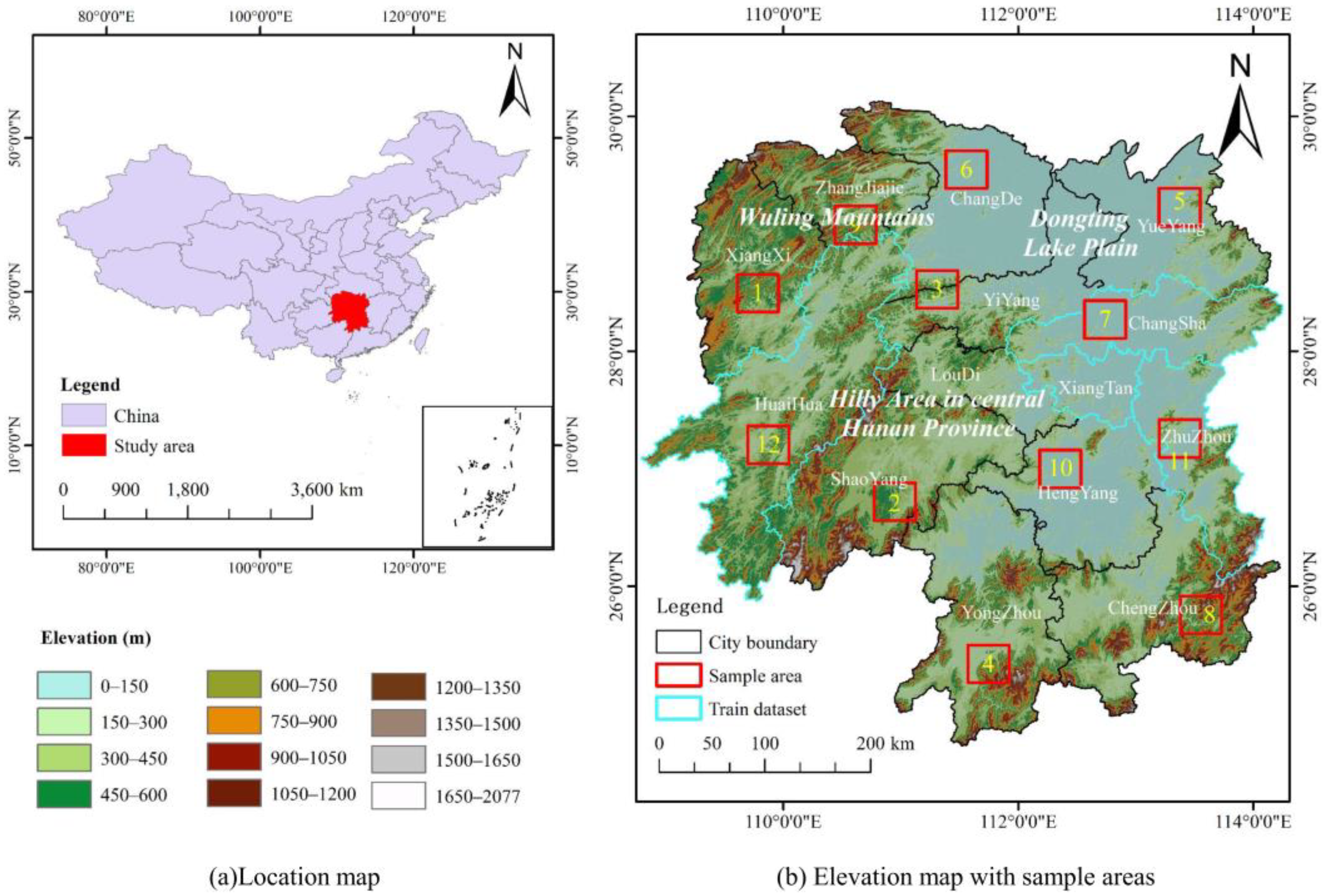
Figure 1. (a) The location of the study area. The full extent of the study area is the satellite image coverage area used for this experiment. (b) The Elevation map of the study area and the location of the sample area distribution. The “train dataset” in the figure is where the training samples are collected.
Remotesensing 15 00628 g001
Figure 2. Woodland Resources Map in Hunan Province.
Remotesensing 15 00628 g002
Figure 3. Flow chart of data preprocessing. The Sentinel-2 L1C images are from ESA and downloaded through the GEE platform. The specific locations where forest change labels were collected were Changsha, Zhuzhou, Xiangtan, and Huaihua in Hunan Province.
Remotesensing 15 00628 g003
Figure 4. Selected cutting samples (256 × 256 pixels). In the label, white values of 255 indicate change, while black values of 0 indicate no change. The first five columns depict changes in forest reduction (column 1 represents forest reduction in mountainous areas, columns 2–4 depict forest reduction in urban areas, and column 5 shows forest reduction due to road construction), while the last two columns show examples of no change.
Remotesensing 15 00628 g004
Figure 5. Copy-paste data augmentation. Copy-paste data augmentation also enriches the diversity of sample backgrounds.
Remotesensing 15 00628 g005
Figure 6. Change detection model (U-Net++).
Remotesensing 15 00628 g006
Figure 7. Post processing diagram. (a) Remove areas of change of less than 667 m2 using the threshold method; (b) Filling of small holes in change areas using the morphological method.
Remotesensing 15 00628 g007
Figure 8. Loss curve for each model.
Remotesensing 15 00628 g008
Figure 9. Comparison of the spatial mapping results for each model; 1–6 columns are for image pairs containing forest changes, and the last column is for image pairs with no changes.
Remotesensing 15 00628 g009
Figure 10. Accuracy metric of each loss function on the test dataset.
Remotesensing 15 00628 g010
Figure 11. Accuracy evaluation chart for each sample area for each year from 2017 to 2021. Sample areas numbered 1, 6, and 9 in 2017, sample areas numbered 1 and 9 in 2018, sample areas numbered 1, 3, 6, and 9 in 2019, and sample area numbered 8 in 2020 are not involved in the accuracy evaluation due to the presence of a large number of clouds.
Remotesensing 15 00628 g011
Figure 12. Results of the quarterly dynamic detection of forest change from 2017 to 2021. A total of 20 periods of Sentinel-2 predictions from 2017 to 2021 yielded a total of 19 forest change detection. No detection is available for this period as no pre-period images were available for spring 2017.
Remotesensing 15 00628 g012
Figure 13. (a) GaoFen satellite images and detection results; (b) Sentinel-2 images and detection results.
Remotesensing 15 00628 g013
Table 1. Data sources.
Data SeriesName of DataData SourceSpatial Resolution (m)Time
Remote sensing dataSentinel-2 L1CEuropean Space Agency
(ESA)
101 January 2017–31 March 2017, 1 April 2017–30 June 2017, 1 July 2017–30 September 2017, 1 October 2017–31 December 2017, 1 January 2018–31 March 2018, 1 April 2018–30 June 2018, 1 July 2018–30 September 2018, 1 October 2018–31 December 2018, 1 January 2019–31 March 2019, 1 April 2019–30 June 2019, 1 July 2019–30 September 2019, 1 October 2019–31 December 2019, 1 January 2020–15 April 2020, 16 April 2020–30 June 2020, 1 July 2020–30 September 2020, 1 October 2020–31 December 2020, 1 January 2021–31 March 2021, 1 April 2021–30 June 2021, 1 July 2021–30 September 2021, 1 October 2021–31 December 2021
Vector dataWoodland Resources MapAcademy of Forestry Inventory and Planning, State Forestry Administration, P.R. China/2020
Administrative boundaryChina Earth System Science Data Sharing Network/2016
Sentinel-2 data are a quarterly composite image. “1 January 2017–31 March 2017” represents all images composited within the spring of 2017.
Table 2. Percentage of positive samples in the dataset.
DatasetTrain DatasetVal DatasetTest DatasetAll Dataset
Number of samples11481441451437
Percentage of positive sample area (%)1.050.941.261.06
Table 3. Accuracy metric of each model on the test dataset.
ModelEncoderLossPrecisionRecallF1-scoreMean Time/min
STANetresnet18CELoss0.70810.63800.67121.55
DeepLabV3+efficientnet-b0CELoss0.77140.71780.743712.35
Linknetefficientnet-b0CELoss0.78540.72200.75240.86
U-Netefficientnet-b0CELoss0.78940.74150.76470.82
U-Net++efficientnet-b0CELoss0.79540.74780.77090.89
Table 4. Evaluation of all sample areas change detection accuracy metrics for 2017–2021.
YearNumber of Sample AreasThe True Area of Change/km2Predicted Area of Change/km2PrecisionRecallF1-score
201787.1646.9480.80910.78480.7968
2018913.50612.7850.85870.81290.8352
2019813.67713.1840.80510.77610.7904
20201112.15112.3120.74940.75930.7543
20211214.60814.2670.83880.81930.8289
Disclaimer/Publisher’s Note: The statements, opinions and data contained in all publications are solely those of the individual author(s) and contributor(s) and not of MDPI and/or the editor(s). MDPI and/or the editor(s) disclaim responsibility for any injury to people or property resulting from any ideas, methods, instructions or products referred to in the content.