A Modification to Phase Estimation for Distributed Scatterers in InSAR Data Stacks

Abstract

To improve the spatial density and quality of measurement points in multitemporal interferometric synthetic aperture radar, distributed scatterers (DSs) should be processed. An essential procedure in DS interferometry is phase estimation, which reconstructs a consistent phase series from all available interferograms. Influenced by the well-known suboptimality of coherence estimation, the performance of the state-of-the-art phase estimation algorithms is severely degraded. Previous research has addressed this problem by introducing the coherence bias correction technique. However, the precision of phase estimation is still insufficient because of the limited correction capabilities. In this paper, a modified phase estimation approach is proposed. Particularly, by incorporating the information on both interferometric coherence and the number of looks, a significant bias correction to each element of the coherence magnitude matrix is achieved. The bias-corrected coherence matrix is combined with advanced statistically homogeneous pixel selection and time series phase optimization algorithms to obtain the optimal phase series. Both the simulated and Sentinel-1 real data sets are used to demonstrate the superiority of this proposed approach over the traditional phase estimation algorithms. Specifically, the coherence bias can be corrected with considerable accuracy by the proposed scheme. The mean bias of coherence magnitude is reduced by more than 29%, and the standard deviation is reduced by more than 18% over the existing bias correction method. The proposed approach achieves higher accuracy than the current methods over the reconstructed phase series, including smoother interferometric phases and fewer outliers.

1. Introduction

Multitemporal interferometric synthetic aperture radar (MT-InSAR) is a powerful technique in monitoring the displacement of Earth’s surface [1,2,3], including a wide range of applications, such as land subsidence [4,5,6], underground mining [7,8], landslide [9,10,11], earthquake [12,13,14], volcanic dynamics [15,16,17] et al. Among various MT-InSAR techniques, the persistent scatterer InSAR (PSInSAR) is a high-precision geodetic approach [18,19]. The basic idea of this technique is to identify and analyze the phase-stable persistent scatterers (PSs) over the whole observation period. These scatterers do not undergo severe temporal decorrelation and usually correspond to man-made objectives. Despite the high precision of PSInSAR, the low spatial density of measurement points, especially over nonurban environments, limits its applications to some extent.

Distributed scatterers (DSs) are exploited to improve the measurement point density. Unlike PS, DS usually covers multiple small targets with the same backscattering behavior in a resolution cell. These targets suffer from geometrical and temporal decorrelation and are typically noisier than those of PSs. To reduce the decorrelation of DS, small baseline subset (SBAS) technique has been proposed by only exploiting interferograms with temporal intervals and spatial baselines smaller than the certain thresholds [20,21,22]. The decorrelation is further reduced by the spatial multi-looking processing. Since the PSs are also filtered with neighboring pixels, their backscattering properties may be contaminated.

To improve the measurement point density by jointly exploiting PSs and DSs, many efforts have been made [22,23,24,25,26], which can be broadly divided into two categories. One is to extend the SBAS technique by combining single-look and multi-look interferograms. PSs can be exploited to achieve fine-scale measurements [22,24]. The other is to extend the PSInSAR technique by adding DSs into the single-master model. The representative work is SqueeSAR [23], and some extended techniques include JSInSAR [27], CAESAR [28], PD-PSInSAR [29], GEOS-ATSA [30], CSI [9] et al. The decorrelation of DS can be significantly reduced by phase estimation.

Initially, the DS phase estimation was implemented based on a maximum likelihood estimator (MLE) [23,31,32], which reconstructs the consistent phase series by maximizing the joint probability density function (pdf) over all pixels in a statistically homogeneous pixel (SHP) set. Theoretically, MLE is the optimum approach for phase estimation. However, the assumptions are difficult to meet in practice, and the optimum performance is compromised. Then the variation is provided by the eigenvalue decomposition (EVD) algorithm [28,29]. Its advantage lies in separating multiple scattering mechanisms, and it has low power for a single scattering mechanism [33,34]. Recently, the eigen decomposition-based maximum-likelihood-estimator of interferometric phase (EMI) algorithm is provided [34]. It follows a similar estimation model as MLE, and has high computational efficiency. These estimators are mathematically compared, and the only difference is the weighting strategy [35]. Based on this, some estimators have been developed with different weights, such as the Fisher information index [36,37], equal weight [35], coherence weight [38,39], coherence power weight [40] et al.

Regardless of the model used by these phase estimation methods, the same data source is the covariance matrix, which is estimated by the maximum-likelihood estimation. As is well known, the estimation is suboptimal due to the heterogeneous samples and limited ensembles [41]. Recently, an alternative way is developed to mitigate the bias by jointly estimating the covariance matrix and the consistent phase series [42]. In general, these influencing factors are treated independently of the phase estimation. In terms of heterogeneous samples, advanced SHP selection algorithms have been developed to reduce the undesirable samples, such as probabilistic method [43], fast SHP selection (FaSHPS) [44], covariance matrix patch (CMP) [45] et al. Robust estimation has also been implemented to mitigate the impact of heterogeneous samples [46]. For limited ensembles, the corresponding covariance matrix usually does not satisfy the positive definiteness, which is required by some estimators for inverse matrix operation [23,34]. Regularization is exploited to solve this problem [47,48,49,50]. In addition, limited ensembles result in a biased covariance matrix, especially for low-coherence areas. The correction by inverting the analytical expression of the coherence magnitude can mitigate the bias [51]. Since the fixed rectangular window is used, the spatial resolution is reduced, and new bias may be introduced. The correction with the second kind of statistical characteristics is introduced to reduce the coherence magnitude bias [52] and shows promising performance [40,53,54]. However, compared with the true coherence, the improvement is inadequate due to the limited correction from a simple bias corrector [53]. Dedicated to accurate deformation monitoring, high-precision phase estimation is still lacking.

In this paper, a new approach is proposed to improve the accuracy of DS phase estimation for InSAR data stacks. Starting from the theoretical analysis of coherence magnitude matrix error, a systematic correction approach is developed by considering the information on both interferometric coherence and the number of looks. Besides, the CMP algorithm is adopted to select SHP set with a high detection rate, and the EMI is exploited to reconstruct the optimal phase series by combining the estimation and computational efficiency. The proposed approach is tested on both simulated and real Sentinel-1 data to demonstrate its effectiveness. The main contributions of this paper are as follows:

(1)

A bias corrector is developed to reduce the error of the coherence magnitude matrix.

(2)

The improvements in coherence bias correction for the state-of-the-art phase optimization algorithms are analyzed and evaluated.

(3)

A processing chain is provided to achieve the high-precision DS phase estimation.

This paper is organized as follows. In Section 2, the related methods are briefly reviewed, and the existing limitation is introduced. We then propose and elaborate on our approach in Section 3. Section 4 is dedicated to the presentation of the experimental results on simulated and real InSAR data stacks. Section 5 presents some discussions. Finally, conclusions are drawn in Section 6.

2. Related Method

Given $N$ co-registered single-look complex (SLC) SAR images, a complex vector $z(x)$ at the position $x$ can be formed as

$$z(x)={[z_1(x),z_2(x),\dots ,z_N(x)]}^T$$

(1)

where ${}^T$ denotes the transpose and $z_i(x)$ is the complex value of the $i$th acquisition at the position $x$.

Based on the central limit theorem, $z$ follows a zero-mean $N$-variate complex circular normal distribution with a covariance matrix $\sum$ [55,56]. The pdf is

$$pdf(z)=\frac{1}{{\pi }^N\det (\sum )}\exp (-z^H{\sum }^{-1}z)$$

(2)

where $\det (\ast )$ indicates the determinant and ${}^H$ stands for Hermitian transpose. When $z$ is normalized such that $E\left({\left|z_i\right|}^2\right)=1$, the corresponding coherence matrix is equal to the covariance matrix [28] and can be estimated as

$$\widehat{T}=\frac{1}{L}{{\displaystyle {\sum }_{k\in \Omega }z(k)z(k)}}^H$$

(3)

where $\Omega$ is the SHP set with $L$ adjacent pixels.

Although the phase of $\widehat{T}$ can be used for unwrapping and deformation retrieval, it is corrupted by the spatiotemporal decorrelation [23]. Phase optimization is developed to minimize the effect of decorrelation by properly combining the information associated with all the interferograms [23,31]. It supposes that the true coherence matrix can be expressed as

$$\Sigma =\Xi \mathsf{\Upsilon }{\Xi }^H$$

(4)

where

$$\Xi =\left[\begin{array}{cccc}{e}^{j{\mathsf{\theta }}_1}& 0& \cdots & 0\\ 0& e^{j{\theta }_2}& \cdots & 0\\ ⋮& ⋮& \ddots & ⋮\\ 0& 0& \cdots & e^{j{\theta }_N}\end{array}\right] \mathsf{\Upsilon }=\left[\begin{array}{cccc}1& {\gamma }_{1,2}& \cdots & {\gamma }_{1,N}\\ {\gamma }_{2,1}& 1& \cdots & {\gamma }_{2,N}\\ ⋮& ⋮& \ddots & ⋮\\ {\gamma }_{N,1}& {\gamma }_{N,2}& \cdots & 1\end{array}\right]$$

where $\Xi$ and $\mathsf{\Upsilon }$ are the true phase and coherence magnitude matrix, respectively. Without loss of generality, ${\theta }_1$ can be set to zero. Therefore, $\mathsf{\theta }={\left[0,{\theta }_2,\dots ,{\theta }_N\right]}^T$ can be termed as the optimal phase series and needs to be estimated. The MLE obtains it by maximizing the joint pdf over all pixels in the SHP set $\Omega$ [23,31,32].

$$\begin{array}{l}{\widehat{\mathsf{\theta }}}_{MLE}=\underset{\mathsf{\theta }}{\arg \max }\left\{{\displaystyle \prod _{k\in \Omega }pdf(z_k)}\right\}\\ =\underset{\mathsf{\theta }}{\arg \max }\left\{{\zeta }^H\left({\mathsf{\Upsilon }}^{-1}\circ \widehat{T}\right)\zeta \right\}\end{array}$$

(5)

where $\zeta ={[1,e^{j{\theta }_2},\dots ,e^{j{\theta }_N}]}^T$ and the symbol $\circ$ represents the Hadamard product. As the true coherence magnitude matrix $\mathsf{\Upsilon }$ is unknown, it is substituted by the absolute of $\widehat{T}$.

$${\widehat{\mathsf{\theta }}}_{MLE}=\underset{\mathsf{\theta }}{\arg \max }\left\{{\zeta }^H\left({\left|\widehat{T}\right|}^{-1}\circ \widehat{T}\right)\zeta \right\}$$

(6)

Equation (6) is a nonlinear optimization problem. Although the Broyden–Fletcher–Glodfarb–Shanno (BFGS) algorithm can be considered as a possible solution, the process is highly time-consuming [23].

Following the MLE, EMI is developed by introducing an additional degree of freedom with the calibration dyadic [34]. Besides, it transforms the nonlinear optimization problem into a minimum eigenvector problem.

$${\widehat{\mathsf{\theta }}}_{EMI}=\underset{u}{\arg \min }\left\{u^H\left({\left|\widehat{T}\right|}^{-1}\circ \widehat{T}\right)u\right\}$$

(7)

where $\widehat{\mathsf{\theta }}=\angle u$, $u$ is the eigenvector of ${\left|\widehat{T}\right|}^{-1}\circ \widehat{T}$.

Compared with the MLE method, EMI is proven to be a more effective method, especially in terms of computational efficiency [34]. It is adopted in our proposed phase estimation algorithm, and the rationality can be found in Section 5.

As analyzed in [35], state-of-the-art phase estimation techniques adopt a similar mathematical model, such as MLE [23,31], EVD [28,29], EMI [34] and the nonlinear optimization estimation weighted with the Fisher information matrix (NLEFIM) [36]. The fundamental difference is the weight matrix, which assigns different weights to different interferograms. Furthermore, these weight strategies require the true coherence magnitude matrix $\mathsf{\Upsilon }$, which is replaced by $\left|\widehat{T}\right|$. As is well-known, Equation (3) is a suboptimal estimator, and the estimated coherence magnitude is biased [55]. The unsatisfactory factor makes the weight matrix inaccurate, resulting in severe damage to the accuracy of the estimated phase series $\widehat{\mathsf{\theta }}={\left[0,{\widehat{\theta }}_2,\dots ,{\widehat{\theta }}_N\right]}^T$.

3. Methodology

In this section, the statistical characteristics of coherence magnitude bias are first analyzed. Then a systematic approach is developed to reduce the coherence bias. In the end, the bias-corrected coherence is combined with advanced SHP selection and phase optimization to obtain the consistent phase series.

3.1. Coherence Magnitude Bias Statistics

Let $\widehat{\gamma }$ be an element of the coherence magnitude matrix $\left|\widehat{T}\right|$; its pdf can be expressed as a function of the true coherence magnitude $\gamma$; and the number of looks $L$ as [57]

$$pdf(\widehat{\gamma }|\gamma ,L)=2(L-1){(1-{\gamma }^2)}^L\widehat{\gamma }{(1-{\widehat{\gamma }}^2)}^{L-2}{}_{2}F_1(L,L;1;{\gamma }^2{\widehat{\gamma }}^2)$$

(8)

where $F$ is the generalized hypergeometric function. Based on the pdf, the analytical expression of the expectation and standard deviation of $\widehat{\gamma }$ can be derived as [58]

$$E(\widehat{\gamma })=\frac{\Gamma (L)\Gamma (3/2)}{\Gamma (L+1/2)}{}_{3}F_2(3/2,L,L;L+1/2,1;{\gamma }^2){(1-{\gamma }^2)}^L$$

(9)

$$D(\widehat{\gamma })={\left(\frac{\Gamma (L)\Gamma (2)}{\Gamma (L+1)}{}_{3}F_2(2,L,L;L+1,1;{\gamma }^2){(1-{\gamma }^2)}^L-{\left(E(\widehat{\gamma })\right)}^2\right)}^{1/2}$$

(10)

where $\Gamma$ is the gamma function.

Equations (9) and (10) are calculated numerically. The difference between the expectation of sample coherence magnitude $E(\widehat{\gamma })$ and true coherence $\gamma$ is displayed in Figure 1a. It can be seen that the $E(\widehat{\gamma })$ is biased towards higher values, and the bias increases with the decrease of $\gamma$ and $L$. Figure 1b shows the standard deviation of sample coherence magnitude $D(\widehat{\gamma })$. It is clear that $D(\widehat{\gamma })$ varies significantly with both $\gamma$ and $L$. The lower the number of looks, the higher the standard deviation. Although the bias can be corrected by inverting Equation (9), the required condition with low $D(\widehat{\gamma })$, corresponding to a sufficiently large $L$, is difficult to meet in practice.

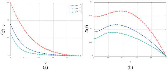
Figure 1. (a) The difference between the expectation of sample coherence magnitude and true coherence $\gamma$ for different numbers of looks $L$. (b) The standard deviation of sample coherence magnitude $D(\widehat{\gamma })$ for different numbers of looks $L$.

Based on the above analysis, a bias corrector should be designed with consideration of the differences at different coherence magnitudes and numbers of looks.

3.2. Bias Mitigation for Coherence Magnitude

The Mellin transform is a valuable tool to analyze the pdf defined on the positive real number field. Based on the second kind second characteristic function, the Mellin transform allows the second kind moment $M_s$ to follow the relation [52]

$$M_s={{\displaystyle {\int }_0^1\left(\ln (\widehat{\gamma })\right)}}^{s}pdf(\widehat{\gamma }|\gamma ,L)d\widehat{\gamma }$$

(11)

The above equation can also be termed as log moment $E\left({\left(\ln (\widehat{\gamma })\right)}^s\right)$. Thus, by inverting Equation (11), an estimator with the corrected coherence magnitude $\tilde{\gamma }$ can be theoretically obtained as

$$\tilde{\gamma }=\exp \left({\left(-1\right)}^{s+1}{\left(M_s\right)}^{1/s}\right)$$

(12)

Section 3.1 shows that the bias of sample coherence magnitude $\widehat{\gamma }$ is related to true coherence magnitude $\gamma$ and the number of looks $L$. Here, the two factors are also considered. Based on the numerical calculation, the difference between the estimated coherence magnitude $\tilde{\gamma }$ and true coherence magnitude $\gamma$ is plotted in Figure 2. It can be seen that the value of $s$ has an important influence on the bias of the estimated $\tilde{\gamma }$. In general, to obtain a more accurate $\tilde{\gamma }$, $s$ should be assigned a larger value when the true coherence $\gamma$ is lower and the number of looks $L$ is smaller. Thus, the value of $s$ should be assigned carefully. Besides, when the parameter is set to the constant $s=1$, the estimator (12) shares a simple form and is previously tested in [40,53,54]. In this paper, it is denoted by $\overline{\gamma }$ and is considered for comparison in the experimental section.

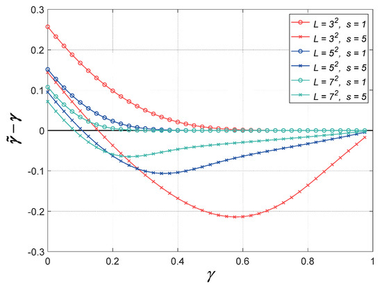
Figure 2. The difference between the estimated coherence magnitude $\tilde{\gamma }$ and true coherence magnitude $\gamma$ for different numbers of looks $L$ and parameters $s$, using numerical calculation.

As the integral of Equation (11) is difficult to realize in practice, the log moment can be approximated by a statistical average over a large number of independent samples. Here, the SHP set $\Omega$ is used to ensure that the samples are independent and identically distributed. The log moment can be approximated as

$$M_s\approx \frac{1}{L}{{\displaystyle {\sum }_{k\in \Omega }\left(\ln \left(\widehat{\gamma }(k)\right)\right)}}^s$$

(13)

From the qualitative analysis in Figure 2, we know that $s$ should be assigned a value that is inversely proportional to both the true coherence magnitude $\gamma$ and the number of looks $L$. To obtain a quantified solution formula for $s$, the values of $\gamma$, $L$ and $s$ are differentiated over a large range into small intervals. The theoretical $\tilde{\gamma }$ is numerically calculated using Equations (11) and (12). Aiming at the minimum difference between $\tilde{\gamma }$ and $\gamma$, the optimal $s$ can be determined as

$$s=\{\begin{array}{ll}1\hfill & \gamma L>5\hfill \\ \left[7-\gamma L\right]\hfill & 1<\gamma L\le 5\hfill \\ 6\hfill & \gamma L\le 1\hfill \end{array}$$

(14)

where $[\ast ]$ rounds down to an integer. Although $s$ should be assigned a larger value when $\gamma L\le 1$, the upper limit is set to 6 with the consideration of the limited accuracy improvements from larger values. In general, the number of looks $L$ is not equal to the sample number. As Equation (14) is an approximate relationship and is not strict, the number of SHP set is used. The true coherence magnitude $\gamma$ is unknown and needs to be estimated. Considering the variance of sample coherence magnitude $\widehat{\gamma }$ is relatively large, taking it as $\gamma$ would result in an inaccurate $s$. Here, an empirical coherence magnitude is pre-estimated to replace $\gamma$.

$$\widehat{\Gamma }={\widehat{\Gamma }}_{thermal}{\widehat{\Gamma }}_{geom}{\widehat{\Gamma }}_{temp}$$

(15)

where

$$\begin{array}{l}{\widehat{\Gamma }}_{thermal}={(1+SN{R}^{-1})}^{-1}\hfill \\ {\widehat{\Gamma }}_{geom}=\max (1-\left|B_{\perp }\right|/B_{\perp \max },0)\hfill \\ {\widehat{\Gamma }}_{temp}=\exp (-B_T/B_{T\max })\hfill \end{array}\}$$

where ${\widehat{\Gamma }}_{thermal}$ is the thermal decorrelation, in which the signal-to-noise ratio (SNR) depends on system parameters and is usually assumed to be a constant value [58]. ${\widehat{\Gamma }}_{geom}$ is the geometric decorrelation. $B_{\perp }$ is the perpendicular baseline, and $B_{\perp \max }$ is the spatial decorrelation baseline, which corresponds to zero correlation [58]. ${\widehat{\Gamma }}_{temp}$ is the temporal decorrelation, and the $B_T$ and $B_{T\max }$ are the temporal baseline and decorrelation rate [58]. The three parameters, including $SNR$, $B_{\perp \max }$ and $B_{T\max }$, are specified in Section 4.1.

As the empirical coherence magnitude $\widehat{\Gamma }$ is a constant value for a single interferometric image, the sample coherence of each pixel can be appropriately corrected by different numbers of looks. The constant $\widehat{\Gamma }$ also ensures that the computational cost is not too high. In addition, the empirical coherence magnitude $\widehat{\Gamma }$ shares different values in different interferograms. For a single pixel, each element of $\left|\widehat{T}\right|$ can be corrected by the corresponding average coherence level. Therefore, the proposed algorithm can achieve effective correction for each element of all sample coherence magnitude matrices. In addition, compared to the sample coherence magnitude $\widehat{\gamma }$ using only SHPs within the search window, the proposed approach actually exploits more pixels, including not only those inside the search window but also those outside the window, which also contributes to reducing the bias of estimated coherence magnitude $\tilde{\gamma }$.

3.3. Phase Estimation Algorithm

Since the SHP set is not only used in Eqation (1) to estimate the sample coherence but also used in Equations (13) and (14) to correct the coherence magnitude bias, it requires to be identified precisely. The CMP algorithm exploits complex information and maintains high accuracy in different sizes of data stacks [45]. It is adopted in this paper to select SHPs.

$$f_{CMP}(x_1,x_2)=\exp \left(-\frac{1}{M}{\displaystyle \sum _{i=1}^M\frac{4}{\pi }\left(\frac{{\widehat{I}}_1^2+{\widehat{I}}_2^2}{{\widehat{I}}_1{\widehat{I}}_2}\left(\frac{1-{\widehat{T}}_i^2\cos ({\widehat{\varphi }}_{1,i}-{\widehat{\varphi }}_{2,i})}{1-{\widehat{T}}_i^2}\right)-2\right)}\right)$$

(16)

where the subscripts 1 and 2 correspond to two pixels with a search window. $M$ interferometric pairs are generated, and ${\widehat{\varphi }}_i$ is the $i$th original interferometric phase. $\widehat{I}$ is the temporal mean intensity and can be estimated as $\widehat{I}={\displaystyle {\sum }_{j=1}^N{I}_j/N}$. $\widehat{T}=h\widehat{\Gamma }$ is an empirical coherence, where $h$ acts as a factor to balance $\widehat{\Gamma }$ and ${\widehat{\varphi }}_i$. Based on a pre-defined threshold, the homogeneity of two pixels can be judged by whether $f_{CMP}$ is greater than the threshold.

The whole procedure of the proposed phase estimation algorithm can be described as follows (see Figure 3).

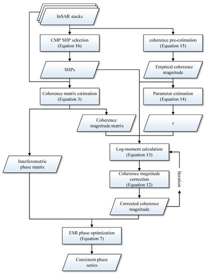
Figure 3. Flowchart of the proposed phase estimation algorithm.

(1)

Apply the CMP algorithm to select SHP set $\Omega$ for each image-pixel $p$.

(2)

Estimate the coherence matrix $\widehat{T}$ using the selected SHP set $\Omega$ and Equation (3).

(3)

Pre-estimate the empirical coherence magnitude $\widehat{\Gamma }$ based on the InSAR stack information and Equation (15).

(4)

Determine parameter $s$ with empirical coherence magnitude $\widehat{\Gamma }$, SHP set $\Omega$ and Equation (14).

(5)

Estimate the log moment $M_s$ using the sample coherence magnitude $\widehat{\gamma }$, parameter $s$ and Equation (13).

(6)

Calculate the corrected coherence magnitude $\tilde{\gamma }$ with the log moment $M_s$ and Equation (12).

(7)

Reconstruct the consistent phase series using EMI and the bias-corrected coherence matrix.

Note that the proposed approach with coherence magnitude bias correction can be termed a general strategy and can be used in other DS phase estimators, such as MLE, EVD and NLEFIM. In practice, Equation (13) is calculated with a limited number of samples, which is generally difficult to meet the assumption of a large number of samples. Here, steps 5–6 are performed iteratively to mitigate this conflict. Considering a trade-off between accuracy improvement and computational cost increase, iteration is typically performed twice. When the computational cost is not considered, more iterations are recommended. In addition, the matrix inversion operation is required by EMI. For cases where the coherence matrix is not positive, definite regularization is committed to resolving the occasional problems via gradually adding a small negative eigenvalue of coherence [46].

4. Experimental Results

4.1. Test on Synthetic InSAR Data Stacks

The simulated data are synthesized based on the coherence matrix, in which the coherence magnitude can be derived as [59]

$$\gamma =({\gamma }_0-{\gamma }_{\propto }){\gamma }_{thermal}{\gamma }_{geom}{\gamma }_{temp}+{\gamma }_{\propto }$$

(17)

where ${\gamma }_0$ and ${\gamma }_{\propto }$ are the short-term and long-term coherence, and are set to 0.7 and 0.03, respectively. ${\gamma }_{thermal}$, ${\gamma }_{geom}$ and ${\gamma }_{temp}$ are the thermal, geometric, and temporal decorrelation, and can be calculated using Equation (15). The SNR is set to 12 dB, resulting in ${\gamma }_{thermal}=0.92$. The perpendicular baselines are normally distributed with a mean of zero and a standard deviation of 50 m, and the spatial decorrelation baseline is 1100 m. The revisiting time and radar wavelength, similar to Sentinel-1, are set to 12 days and 56 mm, respectively. The decorrelation rate is 200 days. The interferometric phases are only related to displacement with a velocity of 1 mm/year. The true data of interferometric phase matrix and coherence magnitude matrix are displayed in Figure 4a,b, respectively. Based on the complex coherence matrix, a stack of 40 images is simulated using a similar procedure to simulate polarimetric SAR images [60]. The size of the simulated image is $100\times 100$ pixels. In addition, since the $\widehat{\Gamma }$ in Equation (15) is an average coherence, the $SNR$, $B_{\perp \max }$, and $B_{T\max }$ are empirically set to 12 dB, 1100 m and 200 days, respectively.

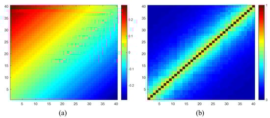
Figure 4. True data of (a) interferometric phase matrix and (b) coherence magnitude matrix.

The values of $s$ with a window of $5\times 5$ and $7\times 7$ pixels are shown in Figure 5, corresponding to the coherence matrix. From Figure 5a, it can be seen that $s$ increases as the coherence magnitude decreases. Comparing Figure 5a,b, it can be found that $s$ is larger when the sample number is smaller. These results are consistent with the theoretical analysis in Section 3.2, indicating the effectiveness of calculating $s$.

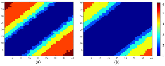
Figure 5. The value of $s$ with a window of (a) $5\times 5$ pixels and (b) $7\times 7$ pixels.

Figure 6 shows the results of coherence matrix estimation with a window of $5\times 5$ pixels. Comparing the true data in Figure 4b and the sample coherence magnitude $\widehat{\gamma }$ in Figure 6a, overestimation can be clearly observed, and it is more severe over the low coherence interferogram. Correcting bias with the method proposed in [53], the coherence magnitude is improved to some extent. Nevertheless, overestimation can still be seen. By performing the correction method proposed in this paper, the coherence magnitude is significantly improved and asymptotically approaches the true data.

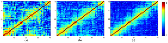
Figure 6. Coherence matrix estimation with a window of $5\times 5$ pixels. (a) Sample coherence magnitude $\widehat{\gamma }$. (b) Corrected coherence magnitude $\overline{\gamma }$. (c) Corrected coherence magnitude $\tilde{\gamma }$ with the proposed method.

To further quantitative evaluation, the means and standard deviations of the estimated coherence magnitude are calculated from all $N(N-1)/2$ interferograms and all pixels, and shown in Figure 7. Considering that the pixel number of SHP set of a DS generally has a threshold [23], e.g., $L>20$, two windows with size of $5\times 5$ and $7\times 7$ pixels are set. From the means in Figure 7a, the overestimation by the sample coherence $\widehat{\gamma }$ can also be observed, and it is more severe when the number of looks is smaller. The mean bias is reduced by 64% by the correction coherence $\overline{\gamma }$ proposed in [53] over the sample coherence $\widehat{\gamma }$. Compared with it, our proposed method achieves a significantly better correction with a bias reduction of more than 29% over the correction coherence $\overline{\gamma }$. This is mainly because that $s$ is appropriately assigned by considering the information on both interferometric coherence and the number of looks. In addition, comparing the standard deviations in Figure 7b, an average reduction of 33% by the corrected coherence $\overline{\gamma }$ over the sample coherence $\widehat{\gamma }$, and 45% by the proposed coherence $\tilde{\gamma }$. The improvement of $\tilde{\gamma }$ over $\overline{\gamma }$ is more than 18%. The lower biases and standard deviations indicate that the proposed method achieves more accurate coherence magnitude estimation. The qualitative and quantitative results jointly demonstrate the effectiveness of the proposed method in correcting the bias of coherence magnitude matrix, especially over the low coherence region.

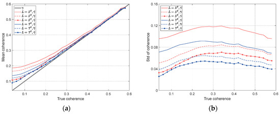
Figure 7. (a) Means and (b) standard deviations for different coherence magnitude estimators using different numbers of looks.

The empirical standard deviation of phase residuals is calculated to provide the quantitative evaluation of phase optimization results. For $i$th image ($i\ne 1$), it is defined as

$$st{d}_i=\sqrt{\frac{1}{K}{\displaystyle \sum _{j=1}^K{(R_{i,j}-{\overline{R}}_i)}^2}}$$

(18)

$$R_{i,j}=\arg \left(\exp \left(j({\widehat{\theta }}_{i,j}-{\theta }_{i,j})\right)\right)$$

(19)

where $K$ is the total number of pixels of the simulated data. $R_{i,j}$ is the residual of the $i$th image and $j$th pixel. ${\widehat{\theta }}_{i,j}$ and ${\theta }_{i,j}$ are the reconstructed phase and the truth value. $\arg (\ast )$ denotes the argument of a complex number. ${\overline{R}}_i$ is the mean residual of the $i$th image and can be estimated as $\frac{1}{K}{\displaystyle {\sum }_{j=1}^K{R}_{i,j}}$. The smaller $std$ means that the reconstructed phase is closer to the truth data.

To evaluate the improvement of coherence magnitude bias correction on phase optimization, different coherence magnitude matrices are used based on the EMI algorithm, and the corresponding standard deviations of residuals are displayed in Figure 8. The theoretically highest achievable precision is provided by the Cramér–Rao lower bound (CRLB) [32]. In general, for different methods, the precision of the phase optimization is higher when the number of looks is larger. This is because more samples can obtain a more accurate complex coherence matrix, including more accurate coherence magnitudes and interferometric phases. Comparing the results with different coherence, it can be found that the coherence magnitude has a noticeable influence on the accuracy of phase optimization. The reconstructed phase with coherence magnitude $\tilde{\gamma }$ proposed in this paper has a higher precision than that with coherence magnitude $\overline{\gamma }$ and approaches the result with true coherence magnitude $\gamma$. The average phase residual with $\tilde{\gamma }$ is 0.11 rad lower than that with $\overline{\gamma }$. In addition, the reconstructed phases with $\tilde{\gamma }$ have a higher precision, an average residual reduction of 0.48 rad, than traditional sample coherence magnitude $\widehat{\gamma }$. This is equivalent to 2.4 mm deviations for the C-band of Sentinel-1, which can lead to a noticeable difference in deformation results. The simulation results demonstrate the effectiveness of performing coherence magnitude bias correction for phase optimization and the superiority of the proposed coherence bias correction method over the existing correction method in phase optimization.

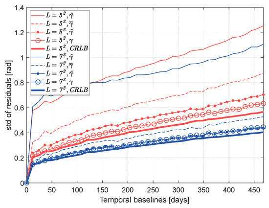
Figure 8. Standard deviation of the residuals for reconstructed phase series using different coherence magnitude estimators. The colors indicate the number of looks.

The reconstructed phase series can be further evaluated by the multi-looking results of a single point. Figure 9 shows the results at any point and the true data. It can also be seen that the reconstructed phases from more samples are closer to the true data. In addition, the reconstructed phases with $\tilde{\gamma }$ have slightly higher precision than that with $\overline{\gamma }$ and are significantly more accurate than that with $\widehat{\gamma }$. The results further demonstrate that the proposed approach can obtain more accurate reconstructed phase series.

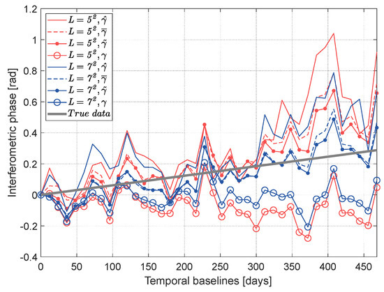
Figure 9. Reconstructed phase series of a single point using different coherence magnitude estimators. The colors indicate the number of looks.

4.2. Test on Real InSAR Data Stacks

A stack of 40 Sentinel-1 images over the Volcán Alcedo is used to test the performance of the proposed algorithm. Figure 10 shows the optical and averaged SAR intensity data, revealing the variety of land cover in the scene. Sentinel-1 images are obtained in wide-swath mode and VV polarization, and from January 2021 to May 2022 in a descending orbit. The test region is limited to an area of $650\times 2400$ pixels. The CMP algorithm is exploited to select SHPs in a $7\times 13$ path. Only pixels with more than 20 SHPs are selected as DS candidates for phase estimation.

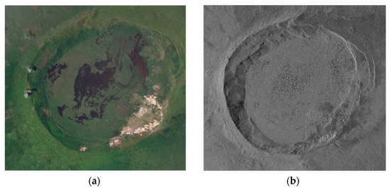
Figure 10. Study area in Volcán Alcedo. (a) Optical image from Google Earth. (b) Averaged intensity map from 40 SLCs of the Sentinel-1 image stacks.

The performance of the proposed approach is visually assessed by inspecting the reconstructed interferograms with the longest temporal baseline of 288 days. The results are displayed in Figure 11. To better compare the details, a selected caldera indicated by the red rectangle is enlarged. A comparison of Figure 11a,b reveals a significant noise suppression of traditional EMI phase optimization. By adopting the corrected coherence magnitude $\overline{\gamma }$, the results are improved with smoother interferometric phases. However, some noise points can still be clearly observed in Figure 11c. The result using the corrected coherence magnitude $\tilde{\gamma }$ proposed in this paper is displayed in Figure 11d, which yields better reconstructed phases with fewer noise points..

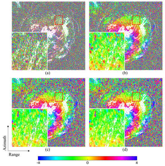
Figure 11. The original and reconstructed interferometric phases with the longest temporal baseline of 288 days. An area denoted by the red rectangle is enlarged. (a) Original single look interferogram. Reconstructed phases using: (b) the sample coherence magnitude $\widehat{\gamma }$, (c) the corrected coherence magnitude $\overline{\gamma }$, (d) the corrected coherence magnitude $\tilde{\gamma }$ proposed in this paper.

The reconstructed interferograms can be further visualized by profile analyses. Figure 12 presents the profiles of original and reconstructed interferograms along the horizontal and vertical black solid lines depicted in Figure 11a. We can see that the profile lines from the corrected coherence magnitude $\overline{\gamma }$ are smoother than those from the sample coherence magnitude $\widehat{\gamma }$, but still contain some outliers. Evidently, the proposed approach with the corrected coherence magnitude $\tilde{\gamma }$ generates smoother profiles with fewer outliers. The better performance indicates the effectiveness of the proposed approach, and can be attributed to the effective correction of coherence magnitude bias.

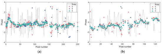
Figure 12. (a) Horizontal and (b) vertical profiles of original and reconstructed interferometric phases along solid black lines depicted in Figure 11a.

Furthermore, a quantitative evaluation of the reconstructed phases is provided by the temporal coherence, which reads as [23]

$${\gamma }_{PTA}=\frac{2}{N(N-1)}{\displaystyle \sum _{i=1}^N{\displaystyle \sum _{j=i+1}^N\cos ({\widehat{\phi }}_{i,j}-{\widehat{\theta }}_i+{\widehat{\theta }}_j)}}$$

(20)

where ${\widehat{\phi }}_{i,j}$ is the interferometric phase in the coherence matrix $\widehat{T}$. ${\widehat{\theta }}_i$ and ${\widehat{\theta }}_j$ are the reconstructed phase with the phase estimation algorithm. Figure 13 shows the histogram of temporal coherence for phase estimation using different coherence magnitude estimators. Improvements can be clearly found between the corrected coherence magnitude $\overline{\gamma }$ and the sample coherence magnitude $\widehat{\gamma }$ over the low temporal coherence regions ( ${\gamma }_{PTA}<0.2$), where the frequency is reduced to near zero by $\overline{\gamma }$. The low temporal coherence regions ( $0.2<{\gamma }_{PTA}<0.45$) are further improved by the corrected coherence magnitude $\tilde{\gamma }$ proposed in this paper. Visual inspection reveals that these improvements are mainly located in densely vegetated areas with low coherence magnitude, which corresponds to high coherence magnitude bias. The experimental results over real SAR data indicate the proposed phase estimation approach can reconstruct better phase series, including smoother phases, fewer outliers and higher temporal coherence.

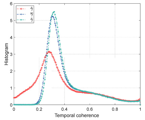
Figure 13. Histogram of temporal coherence for phase estimation using different coherence magnitude estimators.

5. Discussion

The current phase optimization algorithms, such as MLE [23,31], EVD [28,29], EMI [34] and NLEFIM [36], adopt the coherence matrix and its variant as the weight matrix [35]. Thus, the proposed coherence bias correction may be effective for all these phase optimization algorithms. The standard deviation of residuals with the sample coherence magnitude $\widehat{\gamma }$ and bias-corrected coherence magnitude $\tilde{\gamma }$ are displayed in Figure 14. The simulated data in Section 4.1 is adopted and the size of SHP set is $7\times 7$ pixels. It is clear that the corrected coherence magnitude obtains higher accuracy than the traditional sample coherence magnitude. The mean phase residuals are reduced by 0.32 rad, indicating the effectiveness and necessity of performing coherence bias correction. The accuracy improvements of MLE and EVD are more evident than those of EVD and NLEFIM. This is because that the inversion of coherence matrix is executed by the MLE and EMI, which amplify the coherence magnitude bias. When the sample coherence magnitude $\widehat{\gamma }$ is adopted, the NLEFIM is recommended to emphasize estimation accuracy. Since the power of EVD lies in separating scattering mechanisms from different heights, its accuracy is inferior to other methods. For MLE and EMI, the optimum performance can be achieved theoretically when their assumptions are valid. One of the violations of the assumptions is the coherence bias. Thus, the highest accuracy is obtained by MLE and EMI when the bias-corrected coherence magnitude is adopted. Considering that EMI has a computational efficiency advantage over MLE, our proposed phase estimation approach adopts the EMI algorithm.

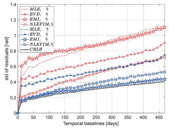
Figure 14. Standard deviation of the residuals for reconstructed phase series using different phase estimators. The colors indicate the coherence matrix estimator used.

To evaluate the computational efficiency, the processing time, including coherence matrix estimation and phase optimization, is provided in Figure 15 over the real data in Section 4.2. The image size is $650\times 2400$ pixels and the search window size is $7\times 13$ pixels. The calculation is in MATLAB R2019a software with an Intel Core I7 processor (3.0 GHz) and 32-GB RAM. In coherence matrix estimation procedure, Since the coherence bias correctors contain the processing of sample coherence estimation, the computational burden increases. The developed corrector is more complex due to the consideration of more information, and takes 2.5 times as long as the previous corrector. During the phase optimization procedure, computation with sample coherence estimation is time consuming. Compared with it, the processing time is improved by 42.2% by that with the previous correction, and by 43.1% by that with the proposed correction. This is because that the additional computation, regarding the coherence matrix regularization, is reduced. Fewer DSs with the non-positive definite coherence matrix are obtained by the developed correction. Considering the total processing time of the proposed approach is high, it is generally recommended for small-sized scenes. In addition, a possible strategy for large-sized images is to introduce high-performance parallel computing technology.

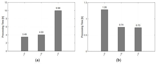
Figure 15. Processing time over: (a) the coherence matrix estimation; (b) the EMI phase optimization.

6. Conclusions

In this article, a modified DS phase estimation has been proposed for InSAR data stacks. The main contribution lies in effectively correcting the bias of coherence magnitude matrix. The core idea is to incorporate the information on both interferometric coherence and the number of looks to adaptively correct each element of the coherence matrix. The proposed approach is established by combing the coherence magnitude bias corrector, the CMP SHP selection and the EMI phase optimization, achieving high-precision phase reconstruction.

The experimental results with the simulated data have shown that more accurate coherence magnitude can be obtained by the proposed correction method, including lower mean bias (reduced by more than 29%) and smaller standard deviation (reduced by more than 18%), than the existing bias correction method. The reconstructed phase series with the proposed approach is closest to the CRLB, demonstrating the effectiveness of the results. The experimental results with the Sentinel-1 images also verify the effectiveness of the proposed approach with smoother interferometric phases and fewer outliers.

References

- Zhu, X.X.; Wang, Y.Y.; Montazeri, S.; Ge, N. A Review of Ten-Year Advances of Multi-Baseline SAR Interferometry Using TerraSAR-X Data. Remote Sens. 2018, 10, 1374. [Google Scholar] [CrossRef]
- Even, M.; Schulz, K. InSAR Deformation Analysis with Distributed Scatterers: A Review Complemented by New Advances. Remote Sens. 2018, 10, 744. [Google Scholar] [CrossRef]
- Minh, D.H.T.; Hanssen, R.; Rocca, F. Radar Interferometry: 20 Years of Development in Time Series Techniques and Future Perspectives. Remote Sens. 2020, 12, 1374. [Google Scholar] [CrossRef]
- Teatini, P.; Tosi, L.; Strozzi, T.; Carbognin, L.; Wegmüller, U.; Rizzetto, F. Mapping regional land displacements in the Venice coastland by an integrated monitoring system. Remote Sens. Environ. 2005, 98, 403–413. [Google Scholar] [CrossRef]
- Hu, J.; Ding, X.L.; Li, Z.W.; Zhang, L.; Zhu, J.J.; Sun, Q.; Gao, G.J. Vertical and horizontal displacements of Los Angeles from InSAR and GPS time series analysis: Resolving tectonic and anthropogenic motions. J. Geodyn. 2016, 99, 27–38. [Google Scholar] [CrossRef]
- Qu, F.; Lu, Z.; Kim, J.-W.; Zheng, W. Identify and Monitor Growth Faulting Using InSAR over Northern Greater Houston, Texas, USA. Remote Sens. 2019, 11, 1498. [Google Scholar] [CrossRef]
- Jiang, L.; Lin, H.; Ma, J.; Kong, B.; Wang, Y. Potential of small-baseline SAR interferometry for monitoring land subsidence related to underground coal fires: Wuda (Northern China) case study. Remote Sens. Environ. 2011, 115, 257–268. [Google Scholar] [CrossRef]
- Perski, Z.; Hanssen, R.; Wojcik, A.; Wojciechowski, T. InSAR analyses of terrain deformation near the Wieliczka Salt Mine, Poland. Eng. Geol. 2009, 106, 58–67. [Google Scholar] [CrossRef]
- Dong, J.; Zhang, L.; Tang, M.; Liao, M.; Xu, Q.; Gong, J.; Ao, M. Mapping landslide surface displacements with time series SAR interferometry by combining persistent and distributed scatterers: A case study of Jiaju landslide in Danba, China. Remote Sens. Environ. 2018, 205, 180–198. [Google Scholar] [CrossRef]
- Zhao, C.; Kang, Y.; Zhang, Q.; Lu, Z.; Li, B. Landslide Identification and Monitoring along the Jinsha River Catchment (Wudongde Reservoir Area), China, Using the InSAR Method. Remote Sens. 2018, 10, 993. [Google Scholar] [CrossRef]
- Intrieri, E.; Raspini, F.; Fumagalli, A.; Lu, P.; Conte, S.D.; Farina, P.; Allievi, J.; Ferretti, A.; Casagli, N. The Maoxian landslide as seen from space: Detecting precursors of failure with Sentinel-1 data. Landslides. 2018, 15, 123–133. [Google Scholar] [CrossRef]
- Wang, R.; Xia, Y.; Grosser, H.; Wetzel, H.U.; Kaufmann, H.; Zschau, J. The 2003 Bam (SE Iran) earthquake: Precise source parameters from satellite radar interferometry. Geophys. J. Int. 2004, 159, 917–922. [Google Scholar] [CrossRef]
- Moreno, M.; Li, S.; Melnick, D.; Bedford, J.R.; Baez, J.C.; Motagh, M.; Metzger, S.; Vajedian, S.; Sippl, C.; Gutknecht, B.D.; et al. Chilean megathrust earthquake recurrence linked to frictional contrast at depth. Nat. Geosci. 2018, 11, 285–290. [Google Scholar] [CrossRef]
- Motagh, M.; Klotz, J.; Tavakoli, F.; Djamour, Y.; Arabi, S.; Wetzel, H.U.; Zschau, J. Combination of Precise Leveling and InSAR Data to Constrain Source Parameters of the M w = 6.5, 26 December 2003 Bam Earthquake. Pure Appl. Geophys. 2006, 163, 1–18. [Google Scholar] [CrossRef]
- Tomiyama, N.; Koike, K.; Omura, M. Detection of topographic changes associated with volcanic activities of Mt. Hossho using D-InSAR. Adv. Space Res. 2004, 33, 279–283. [Google Scholar] [CrossRef]
- Vajedian, S.; Motagh, M.; Nilfouroushan, F. StaMPS Improvement for Deformation Analysis in Mountainous Regions: Implications for the Damavand Volcano and Mosha Fault in Alborz. Remote Sens. 2015, 7, 8323–8347. [Google Scholar] [CrossRef]
- Schaefer, L.N.; Di Traglia, F.; Chaussard, E.; Lu, Z.; Nolesini, T.; Casagli, N. Monitoring volcano slope instability with Synthetic Aperture Radar: A review and new data from Pacaya (Guatemala) and Stromboli (Italy) volcanoes. Earth-Sci. Rev. 2019, 192, 236–257. [Google Scholar] [CrossRef]
- Ferretti, A.; Prati, C.; Rocca, F. Nonlinear subsidence rate estimation using permanent scatterers in differential SAR interferometry. IEEE Trans. Geosci. Remote Sens. 2000, 38, 2202–2212. [Google Scholar] [CrossRef]
- Ferretti, A.; Prati, C.; Rocca, F. Permanent scatterers in SAR interferometry. IEEE Trans. Geosci. Remote Sens. 2001, 39, 8–20. [Google Scholar] [CrossRef]
- Berardino, P.; Fornaro, G.; Lanari, R.; Sansosti, E. A new algorithm for surface deformation monitoring based on small baseline differential SAR interferograms. IEEE Trans. Geosci. Remote Sens. 2002, 40, 2375–2383. [Google Scholar] [CrossRef]
- Goel, K.; Adam, N. An advanced algorithm for deformation estimation in non-urban areas. ISPRS J. Photogramm. Remote Sens. 2012, 73, 100–110. [Google Scholar] [CrossRef]
- Lanari, R.; Mora, O.; Manunta, M.; Mallorqui, J.J.; Berardino, P.; Sansosti, E. A small-baseline approach for investigating deformations on full-resolution differential SAR interferograms. IEEE Trans. Geosci. Remote Sens. 2004, 42, 1377–1386. [Google Scholar] [CrossRef]
- Ferretti, A.; Fumagalli, A.; Novali, F.; Prati, C.; Rocca, F.; Rucci, A. A New Algorithm for Processing Interferometric Data-Stacks: SqueeSAR. IEEE Trans. Geosci. Remote Sens. 2011, 49, 3460–3470. [Google Scholar] [CrossRef]
- Hooper, A. A multi-temporal InSAR method incorporating both persistent scatterer and small baseline approaches. Geophys. Res. Lett. 2008, 35, 96–106. [Google Scholar] [CrossRef]
- Goel, K.; Adam, N. A Distributed Scatterer Interferometry Approach for Precision Monitoring of Known Surface Deformation Phenomena. IEEE Trans. Geosci. Remote Sens. 2014, 52, 5454–5468. [Google Scholar] [CrossRef]
- Perissin, D.; Wang, T. Repeat-Pass SAR Interferometry With Partially Coherent Targets. IEEE Trans. Geosci. Remote Sens. 2012, 50, 271–280. [Google Scholar] [CrossRef]
- Lv, X.; Yazıcı, B.; Zeghal, M.; Bennett, V.; Abdoun, T. Joint-Scatterer Processing for Time-Series InSAR. IEEE Trans. Geosci. Remote Sens. 2014, 52, 7205–7221. [Google Scholar] [CrossRef]
- Fornaro, G.; Verde, S.; Reale, D.; Pauciullo, A. CAESAR: An Approach Based on Covariance Matrix Decomposition to Improve Multibaseline-Multitemporal Interferometric SAR Processing. IEEE Trans. Geosci. Remote Sens. 2015, 53, 2050–2065. [Google Scholar] [CrossRef]
- Cao, N.; Lee, H.; Jung, H.C. A Phase-Decomposition-Based PSInSAR Processing Method. IEEE Trans. Geosci. Remote Sens. 2016, 54, 1074–1090. [Google Scholar] [CrossRef]
- Ge, L.; Ng, A.H.-M.; Li, X.; Abidin, H.Z.; Gumilar, I. Land subsidence characteristics of Bandung Basin as revealed by ENVISAT ASAR and ALOS PALSAR interferometry. Remote Sens. Environ. 2014, 154, 46–60. [Google Scholar] [CrossRef]
- Guarnieri, A.M.; Tebaldini, S. On the Exploitation of Target Statistics for SAR Interferometry Applications. IEEE Trans. Geosci. Remote Sens. 2008, 46, 3436–3443. [Google Scholar] [CrossRef]
- Guarnieri, A.M.; Tebaldini, S. Hybrid Cramér–Rao bounds for crustal displacement field estimators in SAR interferometry. IEEE Signal Process. Lett. 2007, 14, 1012–1015. [Google Scholar] [CrossRef]
- Ansari, H.; Zan, F.D.; Bamler, R. Sequential Estimator: Toward Efficient InSAR Time Series Analysis. IEEE Trans. Geosci. Remote Sens. 2017, 55, 5637–5652. [Google Scholar] [CrossRef]
- Ansari, H.; Zan, F.D.; Bamler, R. Efficient Phase Estimation for Interferogram Stacks. IEEE Trans. Geosci. Remote Sens. 2018, 56, 4109–4125. [Google Scholar] [CrossRef]
- Cao, N.; Lee, H.; Jung, H.C. Mathematical Framework for Phase-Triangulation Algorithms in Distributed-Scatterer Interferometry. IEEE Geosci. Remote Sens. Lett. 2015, 12, 1838–1842. [Google Scholar] [CrossRef]
- Zhao, C.; Li, Z.; Tian, B.; Zhang, P.; Chen, Q. A Ground Surface Deformation Monitoring InSAR Method Using Improved Distributed Scatterers Phase Estimation. IEEE J. Sel. Top. Appl. Earth Obs. Remote Sens. 2019, 12, 4543–4553. [Google Scholar] [CrossRef]
- Samiei-Esfahany, S.; Martins, J.E.; Leijen, F.v.; Hanssen, R.F. Phase Estimation for Distributed Scatterers in InSAR Stacks Using Integer Least Squares Estimation. IEEE Trans. Geosci. Remote Sens. 2016, 54, 5671–5687. [Google Scholar] [CrossRef]
- Zhang, B.; Wang, R.; Deng, Y.; Ma, P.; Lin, H.; Wang, J. Mapping the Yellow River Delta land subsidence with multitemporal SAR interferometry by exploiting both persistent and distributed scatterers. ISPRS J. Photogramm. Remote Sens. 2019, 148, 157–173. [Google Scholar] [CrossRef]
- Song, H.; Zhang, B.; Wang, M.; Xiao, Y.; Zhang, L.; Zhong, H. A Fast Phase Optimization Approach of Distributed Scatterer for Multitemporal SAR Data Based on Gauss–Seidel Method. IEEE Geosci. Remote Sens. Lett. 2022, 19, 1–5. [Google Scholar] [CrossRef]
- Li, S.; Zhang, S.; Li, T.; Gao, Y.; Chen, Q.; Zhang, X. An Adaptive Phase Optimization Algorithm for Distributed Scatterer Phase History Retrieval. IEEE J. Sel. Top. Appl. Earth Obs. Remote Sens. 2021, 14, 3914–3926. [Google Scholar] [CrossRef]
- Jiang, M.; Ding, X.; Li, Z. Hybrid Approach for Unbiased Coherence Estimation for Multitemporal InSAR. IEEE Trans. Geosci. Remote Sens. 2014, 52, 2459–2473. [Google Scholar] [CrossRef]
- Vu, P.; Breloy, A.; Brigui, F.; Yan, Y.; Ginolhac, G. Robust Phase Linking in InSAR. IEEE Trans. Geosci. Remote Sens. 2022. in review. [Google Scholar]
- Schmitt, M.; Schönberger, J.L.; Stilla, U. Adaptive Covariance Matrix Estimation for Multi-Baseline InSAR Data Stacks. IEEE Trans. Geosci. Remote Sens. 2014, 52, 6807–6817. [Google Scholar] [CrossRef]
- Jiang, M.; Ding, X.; Hanssen, R.F.; Malhotra, R.; Chang, L. Fast Statistically Homogeneous Pixel Selection for Covariance Matrix Estimation for Multitemporal InSAR. IEEE Trans. Geosci. Remote Sens. 2015, 53, 1213–1224. [Google Scholar] [CrossRef]
- Zhao, C.; Li, Z.; Tian, B.; Zhang, P.; Wenhao, W.U.; Gao, S.; Yu, Y.; Dong, Y. A statistically homogeneous pixel selection approach for adaptive estimation of multitemporal InSAR covariance matrix. Int. J. Appl. Earth Obs. Geoinf. 2022, 110, 102792. [Google Scholar] [CrossRef]
- Wang, Y.; Zhu, X.X. Robust Estimators for Multipass SAR Interferometry. IEEE Trans. Geosci. Remote Sens. 2016, 54, 968–980. [Google Scholar] [CrossRef]
- Zwieback, S. Cheap, Valid Regularizers for Improved Interferometric Phase Linking. IEEE Geosci. Remote Sens. Lett. 2022, 19, 1–4. [Google Scholar] [CrossRef]
- Zwieback, S.; Meyer, F.J. Reliable InSAR Phase History Uncertainty Estimates. IEEE Trans. Geosci. Remote Sens. 2022, 60, 1–9. [Google Scholar] [CrossRef]
- Wang, C.; Wang, X.S.; Xu, Y.; Zhang, B.; Jiang, M.; Xiong, S.; Zhang, Q.; Li, W.; Li, Q. A New Likelihood Function for Consistent Phase Series Estimation in Distributed Scatterer Interferometry. IEEE Trans. Geosci. Remote Sens. 2022, 60, 1–14. [Google Scholar] [CrossRef]
- Even, M. A Study on Algorithms and Parameter Settings for DS Preprocessing. IEEE Geosci. Remote Sens. Symp. 2021, 3975–3978. [Google Scholar] [CrossRef]
- Eppler, J.; Rabus, B.T. Adapting InSAR Phase Linking for Seasonally Snow-Covered Terrain. IEEE Trans. Geosci. Remote Sens. 2022, 60, 1–13. [Google Scholar] [CrossRef]
- Abdelfattah, R.; Nicolas, J. Interferometric SAR coherence magnitude estimation using second kind statistics. IEEE Trans. Geosci. Remote Sens. 2006, 44, 1942–1953. [Google Scholar] [CrossRef]
- Zhao, C.; Li, Z.; Zhang, P.; Tian, B.; Gao, S. Improved maximum likelihood estimation for optimal phase history retrieval of distributed scatterers in InSAR stacks. IEEE Access. 2019, 7, 186319–186327. [Google Scholar] [CrossRef]
- Li, S.; Zhang, S.; Li, T.; Gao, Y.; Zhou, X.; Chen, Q.; Zhang, X.; Yang, C. An Adaptive Weighted Phase Optimization Algorithm Based on the Sigmoid Model for Distributed Scatterers. Remote Sens. 2021, 13, 3253. [Google Scholar] [CrossRef]
- Bamler, R.; Hartl, P. Synthetic aperture radar interferometry. Inv. Probl. 1998, 14, R1–R54. [Google Scholar] [CrossRef]
- Goodman, N.R. Statistical analysis based on a certain multivariate complex Gaussian distribution (an introduction). Ann. Math. Stat. 1963, 3, 152–177. [Google Scholar] [CrossRef]
- Touzi, R.; Lopes, A.; Bruniquel, J.; Vachon, P.W. Coherence estimation for SAR imagery. IEEE Trans. Geosci. Remote Sens. 1999, 37, 135–149. [Google Scholar] [CrossRef]
- Hanssen, R.F. Radar Interferometry Data Interpretation and Error Analysis; Kluwer: Dordrecht, The Netherlands, 2001. [Google Scholar]
- Morishita, Y.; Hanssen, R.F. Temporal Decorrelation in L-, C-, and X-band Satellite Radar Interferometry for Pasture on Drained Peat Soils. IEEE Trans. Geosci. Remote Sens. 2015, 53, 1096–1104. [Google Scholar] [CrossRef]
- Lee, J.S.; Grunes, M.R.; Kwok, R. Classification of multi-look polarimetric SAR imagery based on complex Wishart distribution. Int. J. Remote Sens. 1992, 15, 2299–2311. [Google Scholar] [CrossRef]
Disclaimer/Publisher’s Note: The statements, opinions and data contained in all publications are solely those of the individual author(s) and contributor(s) and not of MDPI and/or the editor(s). MDPI and/or the editor(s) disclaim responsibility for any injury to people or property resulting from any ideas, methods, instructions or products referred to in the content. |
© 2023 by the authors. Licensee MDPI, Basel, Switzerland. This article is an open access article distributed under the terms and conditions of the Creative Commons Attribution (CC BY) license (https://creativecommons.org/licenses/by/4.0/).