Prediction of Cereal Rye Cover Crop Biomass and Nutrient Accumulation Using Multi-Temporal Unmanned Aerial Vehicle Based Visible-Spectrum Vegetation Indices

Abstract

In general, remote sensing studies assessing cover crop growth are species nonspecific, use imagery from satellites or modified unmanned aerial vehicles (UAVs), and rely on multispectral vegetation indexes (VIs). However, using RGB imagery and visible-spectrum VIs from commercial off-the-shelf (COTS) UAVs to assess species specific cover crop growth is limited in the current scientific literature. Thus, this study evaluated RGB imagery and visible-spectrum VIs from COTS UAVs for suitability to estimate concentration (%) and content (kg ha⁻¹) based cereal rye (CR) biomass, carbon (C), nitrogen (N), phosphorus (P), potassium (K), and sulfur (S). UAV surveys were conducted at two fields in Indiana and evaluated five visible-spectrum VIs—Visible Atmospherically Resistant Index (VARI), Green Leaf Index (GLI), Modified Green Red Vegetation Index (MGRVI), Red Green Blue Vegetation Index (RGBVI), and Excess of Greenness (ExG). This study utilized simple linear regression (VI only) and stepwise multiple regression (VI with weather and geographic data) to produce individual models for estimating CR biomass, C, N, P, K, and S concentration and content. The goodness-of-fit statistics were generated using repeated K-fold cross-validation to compare individual model performance. In general, the models developed using simple linear regression were inferior to those developed using the multiple stepwise regression method. Furthermore, for models developed using the multiple stepwise regression method all five VIs performed similarly when estimating concentration-based CR variables; however, when estimating content-based CR variables the models developed with GLI, MGRVI, and RGBVI performed similarly explaining 74–81% of the variation in CR data, and outperformed VARI and ExG. However, on an individual field basis, MGRVI consistently outperformed GLI and RGBVI for all CR characteristics. This study demonstrates the potential to utilize COTS UAVs for estimating in-field CR characteristics; however, the models generated in this study need further development to expand geographic scope and incorporate additional abiotic factors.

1. Introduction

Across the United States, cereal rye (CR) is the most common cover crop species primarily due to its relatively inexpensive seed cost, straightforward management, and winter hardy nature allowing for ground cover throughout the traditional fallow period [1,2]. Additionally, CR scavenges excess soil N leading to reductions in subsurface drainage nitrate (NO₃-N) losses [3,4,5,6], along with providing a host of soil health benefits [7,8,9]. However, the accumulation of CR biomass and the associated nutrients, including carbon (C), nitrogen (N), phosphorus (P), potassium (K), and sulfur (S), could lead to soil fertility imbalances due to soil nutrients being immobilized by soil microbes decomposing CR residues [10]. Furthermore, CR establishment, and biomass and nutrient content are spatially and temporally variable which can increase the complexity of making management decisions for subsequently grown cash crops [11]. Thus, it is critical for producers to be able to quantify CR biomass and nutrient content in-season to make informed fertility management decisions.

Traditional methods of determining CR biomass and nutrient concentration and content include collecting CR shoot biomass from a known area and submitting it for analysis at a plant tissue testing facility. At the testing facility, the CR shoot biomass must be dried, ground, and analyzed on multiple instruments (dry combustion and inductively coupled plasma spectrometry). Traditional CR Biomass and nutrient concentration and content assessment can be time and labor intensive, and costly [12]. Furthermore, with traditional analyses, there is a lag time between sample collection and receiving analysis results, meaning that producers who use CR biomass and nutrient content analysis to make management decisions must wait for results before making decisions at which time the information regarding the CR may become outdated. Therefore, it is critical that a simple method for the rapid assessment of CR biomass and nutrient concentration and content using commercially available products be developed to allow for real-time informed decisions regarding management decisions for cash crops following CR.

Recently, the use of remotely sensed imaging via UAV or satellite in crop scouting and plant health monitoring has become increasingly popular amongst researchers and the production agriculture community [13]. However, assessment of cover crop productivity via UAV imagery has been somewhat limited. Imagery obtained from UAV platforms can be processed within a matter of hours allowing for timely receipt of results accounting for spatial variability that can be used by producers to make informed management decisions. In research employing UAV platforms, the use of visible spectrum vegetation indices (VIs) (i.e., visible atmospherically resistant index, VARI) is less commonly studied relative to multispectral VIs (e.g., normalized difference vegetation index, NDVI) which can require the addition of costly sensors and modifications to the UAV itself. Studies that examine the use of UAVs to monitor plant growth primarily focus on the prediction of biomass and N accumulation [14,15,16,17,18,19]. Others have used satellite imagery coupled with multispectral VIs to estimate cover crop biomass and N concentration and content [20,21,22]. The studies that focus on cover crops primarily rely on multispectral VIs for prediction, are often species nonspecific, and are more commonly conducted using satellite imagery or modified UAV platforms than off-the-shelf UAV platforms with standard RGB sensors.

In addition, there is a dearth of literature examining methods for the prediction of crop P, K, and S accumulation. Studies developed to assess crop P, K, and S status have relied on costly handheld multispectral or hyperspectral sensors to evaluate reflectance bands for computing VIs [23,24,25,26]. However, the use of remotely sensed imaging to assess crop P, K, and S status is limited. Furthermore, no studies have been conducted to evaluate the efficacy of visible-spectrum VIs obtained from imagery collected with commercially available UAV platforms to predict C, P, K, and S concentration and content in cover crops, let alone CR. Accumulation of C, P, K, and S in CR biomass could lead to soil fertility imbalances and soil nutrient immobilization during residue decomposition; thus, rapid estimation of C, P, K, and S content is critical to inform timely nutrient management decisions.

In this study, it was hypothesized that visible-spectrum vegetation indices obtained by commercially available unmanned aerial vehicles outfitted with standard RGB sensors could be used to accurately predict CR biomass, C, N, P, K, and S concentration and content. The specific objectives were to: (i) evaluate multiple visible-spectrum vegetation indices and determine the best predictors of cereal rye biomass, C, N, P, K, and S concentration and content, and (ii) train and test prediction models for cereal rye biomass, C, N, P, K, and S concentration and content.

2. Materials and Methods

2.1. Experimental Site Description

This study was conducted at two Purdue University Agricultural Centers in the state of Indiana. Field 1 was located at the Agronomy Center for Research and Education near West Lafayette, Indiana, and field 2 was located at the Southeast Purdue Agricultural Center near Butlerville, Indiana. The predominant soil series at field 1 were Drummer silty clay loam (fine-silty, mixed, superactive, mesic Typic Endoaquolls) and a Raub–Brenton silt loam (fine-silty, mixed, superactive, mesic Aquic Argiudolls), and the predominant soil series at field 2 were Cobbsfork silt loam (fine-silty, mixed, active, mesic Fragic Glossaqualfs) and Avonburg silt loam (fine-silty, mixed, active, mesic Aeric Fragic Glossaqualfs). At both locations, CR cover crops were drilled at a rate of 56 kg ha⁻¹ following soybean harvest. Cereal rye planting and termination dates are shown in

Table 1. Location and cereal rye management for the two field sites where UAV flights occurred.

Site	Coordinates	Cereal Rye Planting Date	Cereal Rye Termination Date
Field 1	40°29′17.8″N 86°59′38.8″W	18 September 2020	17 April 2021
Field 2	39°02′00.7″N 85°32′05.7″W	9 October 2020	16 April 2021

.

2.2. Ground-Truth Sampling

On the same date as each UAV flight, CR shoot biomass samples (0.25 m²) were collected at 30 locations within the field. Sample locations were distributed throughout the field to capture the range of growth conditions and biomass levels being evaluated with each UAV flight. All biomass sampling locations were surveyed on the day of the sampling using a Trimble AgGPS 542 (Trimble, Sunnyvale, CA, USA) portable GPS base station mounted on a monopod using the real-time kinematic positioning (RTK) GPS technique. After the GPS survey, biomass samples were oven-dried to a constant weight at 60 °C to determine CR shoot biomass, then ground to pass a 2 mm sieve. Dried and ground CR shoot biomass was submitted to United Soils Inc. (Fairbury, IL, USA) for C, N, P, K, and S content. At United Soils Inc., dried and ground plant tissue samples were batched in groups of 19 samples, 2 method controls, and 3 tissue samples of known composition similar to CR residues. Each batch of tissue samples was analyzed for C and N concentration by combustion analysis (LECO CN 828, St. Josephs, MO, USA). To determine P, K, and S concentrations, 300 mg subsamples of the unknown, known, and method control samples from each batch were weighed, mixed with concentrated nitric acid, microwave digested (CEM Mars 6, Matthews, NC, USA), then analyzed via inductively coupled plasma optical emission spectrometry (Perkin Elmer Optima 7500, Chicago, IL, USA) [27,28].

Precipitation and temperature data were collected from the Purdue Mesonet available through the Indiana State Climate Office for both fields for the period from CR planting to final image acquisition. Temperature data was used to calculate growing degree days (GDD) as follows:

$$\mathrm{Growing}\mathrm{Degree}\mathrm{Days}\left(\mathrm{GDD}\right)=\frac{T_{max}+T_{min}}{2}-T_{base}$$

(1)

where $T_{max}$ is daily maximum air temperature bounded at 30 °C, $T_{min}$ is daily minimum air temperature bounded at 0 °C, and $T_{base}$ is the base temperature (0 °C), which represents the minimum temperature at which CR growth will occur [29,30,31]. Cumulative GDD and cumulative precipitation for each field at each sampling date are shown in

Table 2. The sample dates, accumulated growing degree days (GDD), and accumulated precipitation for field 1 and field 2.

Field 1			Field 2
Sample Date	Cumulative GDD	Cumulative Precipitation, mm	Sample Date	Cumulative GDD	Cumulative Precipitation, mm
29 March 2021	1225.2	319.8	3 December 2020	575.0	255.5
6 April 2021	1316.1	322.6	10 December 2020	600.7	255.5
12 April 2021	1408.2	340.1	22 March 2021	976.1	500.1
			1 April 2021	1084.9	550.7
			8 April 2021	1184.2	555.5
			16 April 2021	1286.9	584.0

.

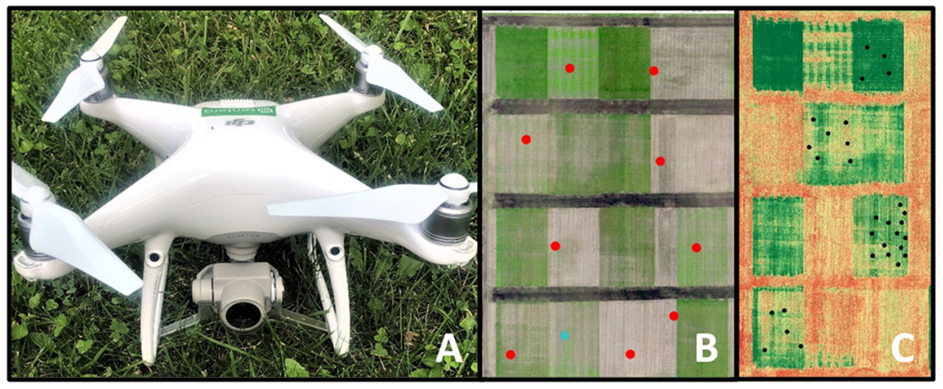
2.3. Unmanned Aerial Vehicle Image Acquisition

The goal of this study was to utilize commercial off-the-shelf (COTS) UAV and software to provide a method of predicting CR biomass and nutrient accumulation applicable to producers, land managers, consultants, and conservation professionals. We used a DJI Phantom 4 Pro (DJI, Shenzhen, China) as a COTS UAV platform to collect aerial imagery in this study (Figure 1). It is equipped with a standard gimble mounted 1-inch 20-megapixel CMOS sensor which has an 84° field-of-view. The RGB sensor captured three separate bands: red (620–700 nm), green (495–570 nm), and blue (450–495 nm). All flights occurred during cloud-free periods between 10:00 am and 11:00 am eastern standard time. The area surveyed was 17 ha for field 1 and 12 ha for field 2, and the survey was completed in a single flight at an altitude of 85 m and a flying speed of approximately 7.25 m S⁻¹. At each field ten ground-control points (GCPs) were evenly distributed for use in enhanced georeferencing during image postprocessing. The GCPs were commercially available 0.25 m² black and white ground targets. Ground control point locations were surveyed via RTK using a Trimble AgGPS 542 portable GPS base station mounted on a monopod.

The number of images collected during each flight was approximately 300 at field 1 and 150 at field 2 and were acquired using a 75% sidelap and 75% frontlap. Collected images were first radiometrically calibrated by capturing images of a MAPIR camera reflectance calibration ground target version 2 (MAPIR, Inc., San Diego, CA, USA) collected just prior to each flight and using the MAPIR Camera Control software (MAPIR, Inc., San Diego, CA, USA) which employs the empirical line method for radiometric correction. Radiometrically calibrated images were then processed using Pix4D fields software (Pix4D SA, Lausanne, Switzerland) to generate 2.3 cm spatial resolution orthomosaic images. Mosaicked images were then georeferenced in ArcGIS Pro (Esri, Redlands, CA, USA) using the control point option within the georeferencing tools resulting in an accuracy level within 0.4 cm. The raster calculator tool within ArcGIS Pro was used to compute vegetation indices.

In this study, five visible-spectrum VIs based on the reflectance values of images at each sampling date including: Visible Atmospherically Resistant Index (VARI), Green Leaf Index (GLI), Modified Green Red Vegetation Index (MGRVI), Red Green Blue Vegetation Index (RGBVI), and Excess of Green (ExG) (

Table 3. Vegetation indices used in this study and their accompanying equations.

Vegetation Index †	Equation ‡	Reference
VARI	$\frac{\left(\rho G-\rho R\right)}{\left(\rho G+\rho R-\rho B\right)}$	[32]
GLI	$\frac{\left(2\times \rho G-\rho R-\rho B\right)}{\left(2\times \rho G+\rho R+\rho B\right)}$	[33]
MGRVI	$\frac{{\left(\rho G\right)}^2-{\left(\rho R\right)}^2}{{\left(\rho G\right)}^2+{\left(\rho R\right)}^2}$	[14]
RGBVI	$\frac{{\left(\rho G\right)}^2-\left(\rho R\times \rho B\right)}{{\left(\rho G\right)}^2+\left(\rho R\times \rho B\right)}$	[14]
ExG	$2\times \rho G-\rho R-\rho B$	[34]

^† VARI = Visible Atmospherically Resistant Index, GLI = Green Leaf Index, MGRVI = Modified Green Red Vegetation Index, RGBVI = Red Green Blue Vegetation Index, and ExG = Excess of Green. ^‡ $\rho G$ is the green reflectance band, $\rho R$ is the red reflectance band, and $\rho B$ is the blue reflectance band.

).

To accurately represent the 0.25 m² CR shoot biomass sampling area, a 0.25 m radius buffer area was created around the georeferenced location of each ground-truth sample. Due to the high spatial resolution of the imagery (0.00053 m² per pixel), each ground-truth buffer area contained between 400 and 500 pixels; thus, the mean VI value from each buffer area was used to build the predictive models. Mean VI values were extracted from the VI maps using the zonal statistics as table tool in ArcGIS Pro.

2.4. Model Cross-Validation and Fitting

Data from all sampling dates at each field were randomly split into training (70%) and testing (30%) datasets, then the datasets from individual fields were combined into singular training and testing datasets to develop the predictive models. This study employed both simplistic and complex methods for the development of predictive models. Independent models were developed using the simplistic and complex methods for both content-based and concentration-based measures of the response variables of CR biomass, CR C, CR N, CR P, CR K, and CR S. The simplistic method used simple linear regression between the in-field measured response variables and the VI values obtained from the UAV flights. This approach represents the most commonly employed method for the prediction of cover crop characteristics within the literature. The general functional form of the simplistic model is described in Equation (2):

RV = β₀ + β₁VI + ε

(2)

where RV is the response variable of CR biomass, CR C, CR N, CR P, CR K, or CR S on either a concentration or content basis, β₀ is the intercept, β₁ is the slope associated with VI, VI is the mean vegetation index (VARI, GLI, MGRVI, RGBVI, or ExG), and ε is an error term.

The complex model is the result of multiple linear regression of the in-field measured response variables against the vegetation index values obtained from the UAV and other exogenous factors including location variables (latitude, longitude, and elevation) and weather variables (accumulated growing degree days and precipitation). These weather variables were selected because they represent the primary drivers of plant growth (temperature and precipitation) and have not been previously included in cover crop biomass and nutrient estimation models. The geographic information included in this study is essentially a proxy for location, however, the authors chose to include it because, when this research is expanded to encompass a larger geographic scope, this information will be more pertinent and help encompass not only location but other factors, such as soil type, drainage, etc. The general functional form of the complex model is described in Equation (3):

RV = β₀ + β₁VI + β₂Long + β₃Lat + β₄Elev + β₅GDD + β₆Precip + ε

(3)

where β_x is the slope associated with the accompanying independent variable, Long is longitude, Lat is latitude, Elev is elevation, GDD is accumulated growing degree days, and Precip is accumulated precipitation.

Repeated K-fold cross validation was used to determine the potential predictive capacity of each VI for each response variable. This method randomly split the data into n subsets known as folds (n = 10), calibrated the model using n-1 folds, then validated the model using the final fold. This calibration-validation procedure was repeated until all folds were used as the validation subset. The process was repeated ten times, with the data randomly redistributed into n number of folds for each iteration. This method was chosen because it is computationally efficient and helps control and minimize bias and variability in the prediction error of the model. This cross-validation procedure produced an average root mean square error (RMSE, presented in the units of measure), normalized RMSE (%RMSE, RMSE as a percentage of the range in the measured data), and adjusted coefficient of determination (Adjusted-R²) for the models. Following cross-validation, concentration and content-based models for each response variable and each VI were fit to the full training dataset. To determine the significance (α = 0.05) of each independent variable within the model, forward stepwise linear regression was performed. Model goodness of fit was determined by assessing the coefficient of determination (multiple-R²), adjusted-R², RMSE, and %RMSE.

3. Results

3.1. Model Cross-Validation and Selection

Summary data of concentration- and content-based in-field CR biomass and nutrients for each field at each flight date are shown in

Table 4. Mean (standard error) of content-based in-field cereal rye biomass and nutrient data collected on the date of each UAV flight.

		Biomass	C	N	P	K	S
Field	Date	Kg ha−1
1	29 March2021	1143 (99)	422 (36)	26.4 (2.3)	2.83 (0.48)	22.8 (2.3)	1.93 (0.16)
	6 April 2021	1762 (144)	651 (52)	37.2 (2.8)	4.90 (0.65)	36.5 (3.5)	2.56 (0.19)
	12 April 2021	1550 (161)	574 (59)	33.4 (3.3)	3.66 (0.62)	34.5 (4.0)	2.25 (0.21)
2	3 December 2020	314 (20)	108 (7)	11.4 (0.6)	1.43 (0.09)	7.17 (0.5)	0.79 (0.04)
	10 December 2020	404 (17)	148 (6)	14.4 (0.5)	1.84 (0.09)	8.59 (0.4)	1.03 (0.04)
	22 March 2021	868 (27)	316 (10)	22.2 (0.9)	2.64 (0.13)	15.5 (0.8)	1.67 (0.06)
	1 April 2021	1193 (62)	432 (22)	25.0 (1.5)	3.81 (0.26)	25.7 (1.6)	1.92 (0.10)
	8 April 2021	1720 (66)	629 (23)	29.7 (1.3)	5.07 (0.35)	36.8 (2.1)	2.40 (0.11)
	16 April 2021	4008 (103)	1469 (37)	58.4 (2.9)	10.79 (0.41)	84.5 (2.8)	4.86 (0.15)

and

Table 5. Mean (standard error) of concentration-based in-field cereal rye nutrient data collected on the date of each UAV flight.

		C	N	P	K	S
Field	Date	%
1	29 March2021	37.1 (0.13)	2.35 (0.07)	0.213 (0.02)	1.95 (0.05)	0.174 (0.004)
	6 April 2021	37.1 (0.12)	2.17 (0.06)	0.202 (0.02)	2.03 (0.03)	0.151 (0.005)
	12 April 2021	37.2 (0.24)	2.22 (0.07)	0.206 (0.01)	2.17 (0.03)	0.151 (0.005)
2	3 December 2020	34.7 (0.31)	3.69 (0.06)	0.454 (0.01)	2.29 (0.03)	0.257 (0.004)
	10 December 2020	36.7 (0.16)	3.59 (0.06)	0.456 (0.01)	2.12 (0.04)	0.255 (0.004)
	22 March 2021	36.4 (0.16)	2.56 (0.06)	0.302 (0.01)	1.76 (0.05)	0.193 (0.003)
	1 April 2021	36.3 (0.10)	2.09 (0.05)	0.316 (0.01)	2.14 (0.06)	0.162 (0.003)
	8 April 2021	36.6 (0.12)	1.72 (0.02)	0.288 (0.01)	2.11 (0.04)	0.139 (0.002)
	16 April 2021	36.6 (0.05)	1.45 (0.05)	0.269 (0.01)	2.11 (0.04)	0.121 (0.002)

, respectively.

Repeated K-fold cross-validation was used to assess the potential predictive capacity of different VIs using both simplistic and complex model development methods on concentration and content-based response variables of CR biomass, C, N, P, K, and S. In general, the models developed using the simplistic method performed relatively poorly (R² = 0.02–0.47); however, the simplistic models developed using content-based CR response variables explained a relatively greater proportion of the variation (R² = 0.04–0.47) in response variables compared to the concentration-based models (R² = 0.02–0.20,

Table 6. Root mean square error (RMSE), %RMSE, and coefficient of determination (R²) for repeated K-fold cross validation of cereal rye biomass (Bio), nutrient concentration, and content-based models for different vegetation indices developed using the simple method.

	Statistic	VARI		GLI		MGRVI		RGBVI		ExG
		Conc	Content	Conc	Content	Conc	Content	Conc	Content	Conc	Content
Bio	Adj. R2		0.04		0.33		0.25		0.35		0.20
	RMSE		1173		983		1038		970		1075
	%RMSE		24%		20%		21%		20%		22%
C	Adj. R2	0.12	0.05	0.04	0.34	0.07	0.25	0.04	0.34	0.05	0.21
	RMSE	1.03	430	1.06	358	1.06	379	1.06	358	1.07	394
	%RMSE	12%	24%	12%	20%	13%	21%	12%	20%	12%	21%
N	Adj. R2	0.02	0.08	0.13	0.47	0.06	0.34	0.13	0.47	0.13	0.26
	RMSE	0.79	17.9	0.75	13.1	0.77	14.9	0.75	13.2	0.75	15.7
	%RMSE	25%	15%	24%	11%	24%	12%	24%	11%	23%	13%
P	Adj. R2	0.15	0.07	0.03	0.37	0.09	0.35	0.03	0.42	0.05	0.19
	RMSE	0.10	3.39	0.11	2.77	0.11	2.80	0.11	2.66	0.11	3.16
	%RMSE	21%	22%	23%	18%	23%	18%	23%	17%	23%	21%
K	Adj. R2	0.04	0.06	0.12	0.39	0.13	0.29	0.12	0.40	0.20	0.24
	RMSE	0.26	25.9	0.25	20.7	0.25	22.4	0.25	20.6	0.24	23.2
	%RMSE	21%	23%	20%	18%	20%	20%	20%	18%	19%	20%
S	Adj. R2	0.05	0.06	0.20	0.38	0.07	0.32	0.17	0.41	0.18	0.21
	RMSE	0.05	1.34	0.05	1.07	0.05	1.13	0.05	1.05	0.05	1.21
	%RMSE	24%	22%	22%	17%	24%	18%	23%	17%	22%	20%

).

Based on these findings, and the fact that the complex models were capable of explaining a substantially larger proportion of the variation in the response variables (R² = 0.16–0.83), the simplistic models were considered inferior, and exploration of these models ended after the initial model development and cross-validation stage.

The complex models developed using concentration-based CR response variables explained 16–83% of the variation in the response variables; however, performance varied based upon the response variable being predicted (

Table 7. Root mean square error (RMSE), %RMSE, and coefficient of determination (R²) for repeated K-fold cross validation of concentration (conc) and content-based cereal rye biomass (Bio) and nutrient accumulation models for different vegetation indices developed using the complex method.

	Statistic	VARI		GLI		MGRVI		RGBVI		ExG
		Conc	Content	Conc	Content	Conc	Content	Conc	Content	Conc	Content
Bio	Adj. R2		0.63		0.78		0.80		0.78		0.61
	RMSE		725		554		556		554		750
	%RMSE		15%		11%		11%		11%		15%
C	Adj. R2	0.16	0.63	0.21	0.78	0.19	0.79	0.20	0.78	0.16	0.62
	RMSE	1.05	266	0.97	208	1.00	203	0.99	205	1.04	272
	%RMSE	12%	15%	11%	12%	12%	11%	12%	11%	12%	15%
N	Adj. R2	0.80	0.50	0.79	0.76	0.79	0.73	0.78	0.77	0.80	0.52
	RMSE	0.35	13.2	0.36	9.11	0.36	9.75	0.37	8.98	0.35	12.7
	%RMSE	11%	11%	11%	8%	11%	8%	12%	7%	11%	10%
P	Adj. R2	0.67	0.55	0.77	0.82	0.73	0.80	0.77	0.83	0.71	0.55
	RMSE	0.07	2.51	0.05	1.50	0.06	1.59	0.05	1.48	0.06	2.44
	%RMSE	14%	16%	10%	10%	11%	10%	11%	10%	12%	16%
K	Adj. R2	0.16	0.61	0.22	0.82	0.22	0.81	0.23	0.82	0.27	0.62
	RMSE	0.28	16.9	0.26	11.1	0.26	11.5	0.25	11.0	0.24	16.5
	%RMSE	22%	15%	21%	10%	21%	10%	20%	10%	19%	15%
S	Adj. R2	0.83	0.56	0.81	0.79	0.81	0.79	0.80	0.79	0.81	0.57
	RMSE	0.02	0.92	0.02	0.63	0.02	0.63	0.02	0.62	0.02	0.91
	%RMSE	10%	15%	10%	10%	10%	10%	10%	10%	10%	15%

).

Poor overall model performance was observed for CR C (adj. R² = 0.16–0.21) and K (adj. R² = 0.16–0.27) concentrations; however, satisfactory predictions of CR N (adj. R² = 0.78–0.80), P (adj. R² = 0.67–0.77), and S (adj. R² = 0.80–0.83) concentrations were achieved using this methodology. All content-based models developed using the complex method were capable of explaining at least 50% (adj. R² = 0.50–0.83) of the variation in the response variables (Table 7). In general, VARI and ExG were relatively poor predictors for all content-based response variables (adj. R² = 0.50–0.63) when compared to GLI, MGRVI, and RGBVI (adj. R² = 0.73–0.83), which all performed relatively similar to each other. Based on these findings, and the relevance of understanding content-based CR biomass and nutrient accumulation to the production agriculture community, GLI, MGRVI, and RGBVI were chosen for further fitting and analysis of both concentration and content-based models.

3.2. Model Fitting and Analysis

To determine the significance of individual independent variables within the fitted models, forward stepwise multiple linear regression was performed. In general, forward stepwise multiple linear regression revealed that VI and GDD were significant in the models for all concentration-based CR response variables except phosphorus, while the significance of longitude, latitude, elevation, and accumulated precipitation within the models varied based upon the response variable. Estimated regression coefficients of model parameters for the C, N, P, K, and S concentration models are shown in

Table 8. Estimated regression coefficients for cereal rye carbon (C), nitrogen (N), phosphorus (P), potassium (K), and sulfur (S) concentration model parameters determined by forward stepwise multiple linear regression (α = 0.05).

	Model VI	Intercept	VI	Long	Lat	Elev	GDD	Precip
C	GLI	28.05	−11.02				0.002	−0.002
	MGRVI	10.54	−5.937	−0.232			0.001
	RGBVI	23.68	−12.78				0.002	−0.002
N	GLI	5.503	−2.811			−0.008	−0.002	−0.002
	MGRVI	7.305	−2.269			−0.016	−0.003
	RGBVI	3.949	−3.786			−0.008	−0.002	−0.001
P	GLI	505.2	1.460	10.58	10.30	−0.004		−0.001
	MGRVI	673.8	0.854	14.21	13.93	−0.005		−0.001
	RGBVI	516.5	1.928	10.80	10.52	−0.004		−0.001
K	GLI	1118	3.521	23.45	22.85		0.001	−0.003
	MGRVI	1335	2.654	28.07	27.43		0.002	−0.003
	RGBVI	1099	4.856	22.99	22.39		0.001	−0.003
S	GLI	−1.045	−0.277		0.032		−0.0002
	MGRVI	−0.402	−0.179			−0.001	−0.0002
	RGBVI	−1.133	−0.362		0.030		−0.0002

.

Forward stepwise multiple linear regression of models developed for content-based CR characteristics showed that VI, GDD, and accumulated precipitation were always significant within the models regardless of CR response variable while elevation was not necessary, and the significance of longitude and latitude were model dependent. Estimates of model parameter regression coefficients for the biomass, C, N, P, K, and S content-based models are shown in

Table 9. Estimated regression coefficients for content-based cereal rye biomass, carbon (C), nitrogen (N), phosphorus (P), potassium (K), and sulfur (S) model parameters determined by forward stepwise multiple linear regression (α = 0.05).

	Model VI	Intercept	VI	Long	Lat	Elev	GDD	Precip
Bio	GLI	162,100	20,100		−3871		9.66	−13.15
	MGRVI	176,598	15,399		−4252		11.54	−16.55
	RGBVI	175,800	27,280		−3926		10.06	−13.91
C	GLI	59,577	7289.7		−1424		3.57	−4.87
	MGRVI	64,866	5603.7		−1563		4.25	−6.10
	RGBVI	64,567	9905.5		−1444		3.71	−5.15
N	GLI	4119	384.25	45.42			0.115	−0.156
	MGRVI	47,630	271.90	978.2	928.7		0.150	−0.218
	RGBVI	4426	518.73	46.45			0.122	−0.170
P	GLI	8331	78.36	169.5	159.2		0.024	−0.033
	MGRVI	14,150	56.06	293.9	282.6		0.031	−0.046
	RGBVI	8260	106.6	166.8	156.3		0.025	−0.036
K	GLI	3718	506.5		−87.93		0.214	−0.302
	MGRVI	8577	381.3	97.12			0.262	−0.387
	RGBVI	4065	688.8		−89.31		0.224	−0.321
S	GLI	162.4	26.26		−3.764		0.009	−0.012
	MGRVI	378.5	20.05	4.251			0.012	−0.017
	RGBVI	180.4	35.71		−3.836		0.010	−0.013

.

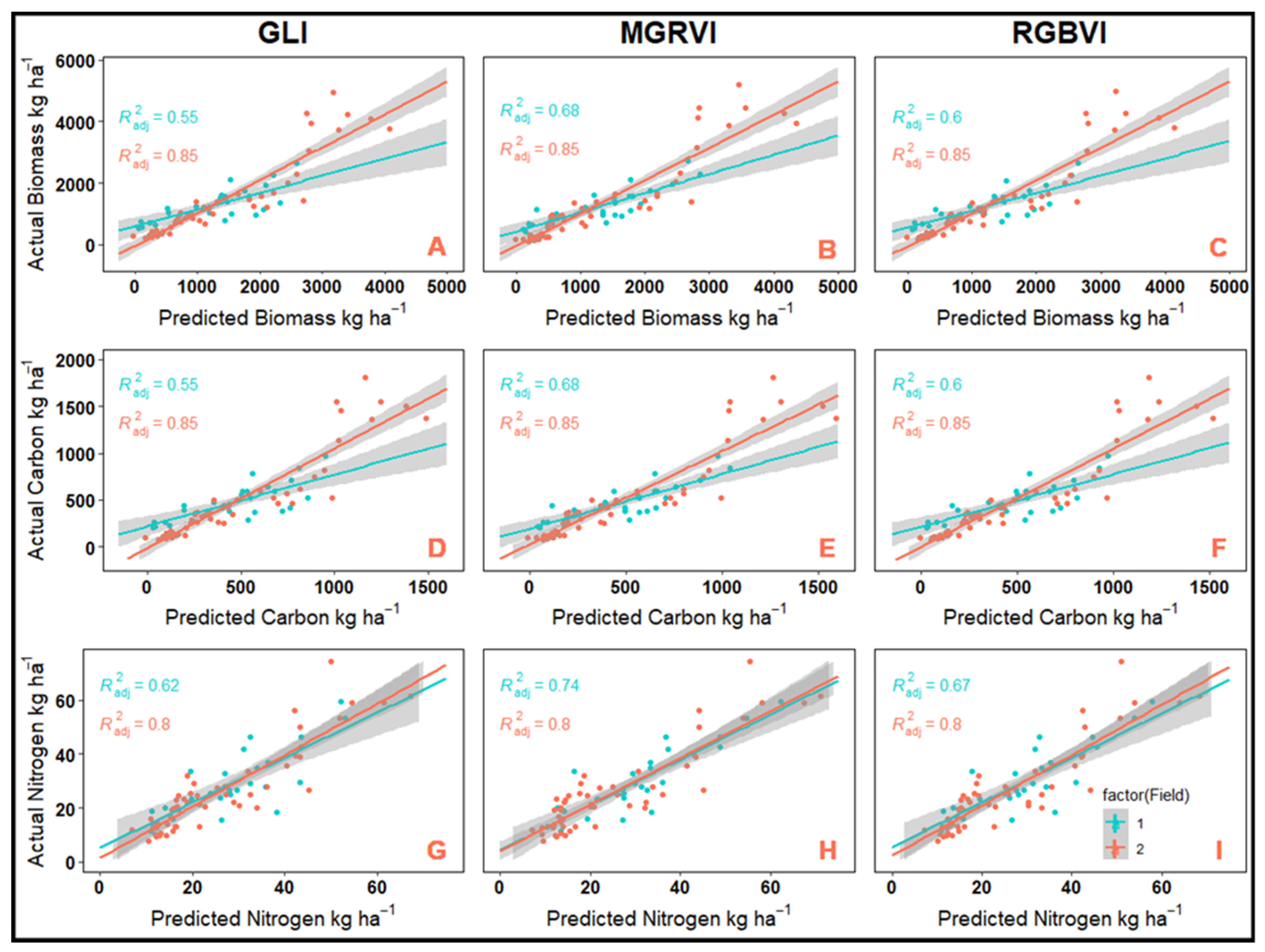
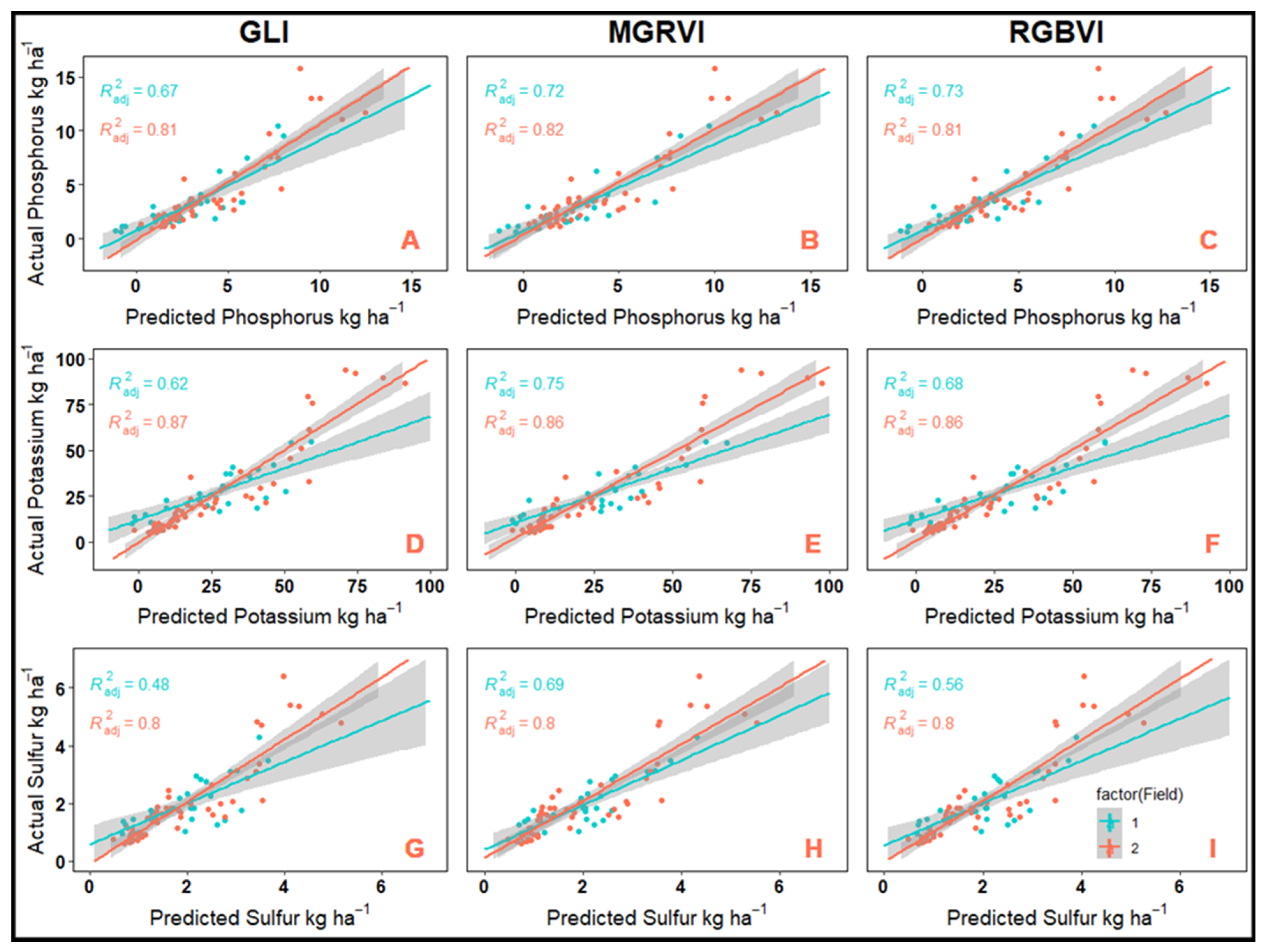
3.3. Final Model Goodness-of-Fit

Following cross-validation and forward stepwise multiple linear regression, the final models were fit for each response variable to the testing data set containing information from both fields. Model goodness of fit was evaluated by the multiple R² and adjusted R² statistics which describe the percent variation in the dependent variable explained by the independent variables. Adjusted R² accounts for the number of independent variables when analyzing the goodness of fit for the model. Large deviation in the adjusted R² statistic from the multiple R² value can indicate overfitting within the model; however, in this study, little to no difference between multiple and adjusted R² statistics was observed indicating that overfitting was not an issue (

Table 10. Multiple R², adjusted R², root mean square error, and percent root mean square error values of the final fitted models for the response variables of cereal rye biomass, carbon, nitrogen, phosphorus, potassium, and sulfur.

Response Variable	Units		Multiple R2	Adjusted R2	RMSE	% RMSE
Biomass	kg ha−1	GLI	0.79	0.79	486	10%
		MGRVI	0.81	0.81	464	9%
		RGBVI	0.80	0.8	480	10%
Carbon	%	GLI	0.35	0.34	1.07	12%
		MGRVI	0.35	0.34	1.07	12%
		RGBVI	0.34	0.33	1.08	13%
	kg ha−1	GLI	0.80	0.79	177	10%
		MGRVI	0.81	0.81	169	9%
		RGBVI	0.80	0.80	175	10%
Nitrogen	%	GLI	0.87	0.87	0.27	10%
		MGRVI	0.87	0.87	0.27	10%
		RGBVI	0.87	0.87	0.27	10%
	kg ha−1	GLI	0.77	0.76	7.08	6%
		MGRVI	0.80	0.79	6.63	5%
		RGBVI	0.78	0.78	6.91	6%
Phosphorus	%	GLI	0.83	0.83	0.05	10%
		MGRVI	0.83	0.83	0.05	11%
		RGBVI	0.84	0.84	0.05	10%
	kg ha−1	GLI	0.78	0.78	1.50	10%
		MGRVI	0.80	0.80	1.44	9%
		RGBVI	0.80	0.79	1.46	9%
Potassium	%	GLI	0.34	0.34	0.22	18%
		MGRVI	0.36	0.35	0.22	18%
		RGBVI	0.35	0.34	0.22	19%
	kg ha−1	GLI	0.79	0.79	10.7	9%
		MGRVI	0.82	0.81	10.1	9%
		RGBVI	0.80	0.80	10.6	9%
Sulfur	%	GLI	0.85	0.85	0.02	10%
		MGRVI	0.84	0.84	0.02	10%
		RGBVI	0.85	0.85	0.02	10%
	kg ha−1	GLI	0.74	0.74	0.64	10%
		MGRVI	0.78	0.77	0.60	10%
		RGBVI	0.78	0.75	0.63	10%

).

In general, the concentration-based models developed in this study performed adequately in the prediction of N (adj. R² = 0.87), P (adj. R² = 0.83–0.84), and S (adj. R² = 0.84–0.85); however, less than 36% of variation in CR C and K concentrations could be explained using these models. In contrast, models developed for content-based CR response variable performed adequately regardless of the characteristic being modeled and were capable of explaining 74–82% of the variation of the in-field measured values (Table 10). Simultaneously, the final trained models for GLI, MGRVI, and RGBVI were fit to the individual testing data sets from each field. In this case, model goodness of fit was determined using the adjusted R² values. In general, the models were able to more accurately predict the data from field 2 (adj. R² = 0.80–0.87) than from field 1 (adj. R² = 0.48–0.75), and the model trained using MGRVI provided better overall predictions than those trained with GLI and RGBVI (Figure 2 and Figure 3)

4. Discussion

4.1. Can Visible Spectrum Vegetation Indices Be Used to Predict Concentration and Content-Based Cereal Rye Biomass and Nutrient Accumulation?

In this study, we evaluated the utility of five visible-spectrum vegetation indices to predict both CR biomass and nutrient concentration and content. The models developed using simple linear regression between visible-spectrum VIs and CR characteristics performed relatively poorly for both concentration-based (R² = 0.02–0.20) and content-based measures of CR characteristics (R² = 0.04–0.47) (Table 6). Contrastingly, the complex models developed in this study including exogenous factors, such as geographic and weather data, provided satisfactory performance for almost all concentration and content-based measures of CR biomass and nutrient accumulation. The adjusted-R² (0.67–0.83) and percent RMSE (10–14%) in cross-validation suggested that all five VIs were capable of predicting concentration-based CR N, P, and S accumulation with reasonable model performance; however, all VIs were insufficient in their predictive capacity of concentration-based CR C and K accumulation (Table 7). Likewise, the adjusted-R² (0.50–0.83) and percent RMSE (7–16%) in cross-validation for the complex models developed using content-based measures of cereal rye biomass and nutrient suggested that all five VIs were capable of predicting CR biomass, C, N, P, K, and S with satisfactory model performance (Table 7). However, in general across all dependent variables, models trained with GLI, MGRVI, and RGBVI explained a greater proportion of variation in the dependent variable compared to those trained with VARI and ExG. The previous literature typically evaluated some combination of visible-spectrum and multispectral VIs to determine the best predictor of crop growth parameters; thus, all five VIs utilized in this study were rarely evaluated at the same time. In contrast to the current study, Barbosa et al. [35] evaluated visible-spectrum VIs in grass production and determined MGRVI was effective at differentiating vegetation from soil, but GLI, RGBVI, and ExG were not. However, they had no method for radiometric correction, and concluded that high radiometric variability of images contributed to the inefficacy of GLI, RGBVI, and ExG. Radiometric variability was controlled for in the current study, which could help explain the low variability between models developed for all five Vis. Likewise, Lussem et al. [16] also reported that RGBVI and GLI were poor predictors of biomass production in grass forage systems and warned that VARI is prone to saturation effects at later growth stages which is a common issue amongst all visible-spectrum and multispectral vegetation indices. Prabhakara et al. [21] also stated that VARI could effectively predict grass cover crop biomass levels at early growth stages, but its predictive capacity was significantly reduced later in the growing season likely due to saturation issues. However, many studies have reported that RGBVI performs moderate to well at predicting biomass levels in grassland production systems [14,15,36]. Specifically, Bareth et al. [36] reported that RGBVI showed high correlation with NDVI, which is one of the most commonly utilized multispectral Vis in agricultural research. From this finding they concluded that visible-spectrum Vis computed from imagery captured by UAVs with RGB sensors could be used to monitor grassland performance. Bendig et al. [14] determined that MGRVI and RGBVI were relatively good at predicting barley biomass accumulation prior to the boot growth stage. Similarly, Yeom et al. [37] concluded that MGRVI was able to reliably discern differences in cotton and sorghum growth across the growing season and tillage treatments and could represent an efficient and economical alternative to multispectral imaging. In the current study, the inclusion of exogenous factors that control crop growth and performance likely reduced the potential impact of any saturation effect on the predictive models, coupled with all UAV flights occurring prior to CR reaching the boot growth stage and transitioning into reproductive growth. Further research is needed to determine if visible-spectrum Vis coupled with weather and geographic data can produce reliable predictions after CR reaches the boot growth stage and proceeds to reproductive growth.

4.2. How Accurately Can Visible-Spectrum Vegetation Indices Predict Cereal Rye Biomass, Carbon, Nitrogen, Phosphorus, Potassium, and Sulfur Concentration and Content?

Goodness-of-fit statistics including adjusted-R² and %RMSE were used to evaluate the trained models for CR biomass and nutrient concentration and content using the complete testing dataset (Table 10). Due to Vis coupled with weather and geographic data produced models with satisfactory performance for all content-based response variables investigated in the current experiment and CR biomass is a content-based measure only, the discussion on model prediction accuracy will focus on the complex models developed using CR biomass and nutrient content.

The CR biomass predictive models developed in this study tested using the complete testing dataset had an adjusted-R² of 0.79 to 0.81 and %RMSE of 9–10%, respectively, meaning that the model explained 80–81% of the variation in the dependent variable and that the difference between predicted and actual values were 9–10% of the range in the measured data. However, when examining model performance on an individual field basis the model trained with each of the vegetation indices had greater predictive capacity for field 2 (adj. R² = 0.85) than field 1 (adj. R² = 0.55–0.68), a trend that held true for all content-based CR response variables (Figure 2A–C). Previous literature evaluating the predictive capacity of visible-spectrum VIs for crop biomass accumulation produced models with R² values of 0.36 to 0.83, though many of these studies were not for cover crops and none were specific to CR [14,15,16,21]. Other studies which evaluated cover crop biomass using multispectral VIs produced models for biomass accumulation with R² values between 0.32 and 0.93, which were comparable to the results obtained in this study using visible-spectrum VIs [18,20,21,22]. However, other studies have showed poor correlation between VIs and cover crop biomass with poor results primarily contributed to small ranges of biomass and VI values collected in the studies [38,39]. The variation in results within the previous literature could be explained by studies demonstrating that the correlation between VIs and crop characteristics decreases as crop growth stage increases [40,41,42,43,44]. Furthermore, much of the previous literature focused on simple linear regression between VIs and crop biomass in order to develop predictive models and used images from a single point in time rather than multitemporal imaging to capture changes in biomass over time. Therefore, the goodness-of-fit for the CR biomass accumulation model in this study could be explained by the multitemporal nature of the imaging, the use of radiometric calibration, the inclusion of geographic and weather data that help control CR growth, and the fact that all imaging occurred prior to reproductive growth while CR was at the early booting stage or younger, helping to avoid issues of VI saturation and radiometric variability observed in other studies [16,35,36].

No studies have been conducted using UAV imagery to compute VIs for the prediction of C accumulation in CR or other crop species. In this study, the C accumulation models that were developed had adjusted-R² values of 0.79 to 0.81 and %RMSE of 9–10%. When tested on individual fields adjusted R² of field 1 was 0.55–0.68 and 0.85 for field 2 (Figure 2D–F). These goodness-of-fit statistics suggest that content-based CR C accumulation can be predicted with relative accuracy using UAV-based RGB imagery coupled with geographic and weather data. Carbon accumulation is strongly correlated to crop biomass production hence the strong similarities between the models for carbon and biomass. Cover cropping can improve average annual soil organic carbon stock increases [45]. Thus, cover cropping is an essential method of potential carbon sequestration in the emerging carbon credit market, which is developed to provide producers employing regenerative agricultural practices with payments per unit of carbon sequestered within their cropping systems. Having a method for rapidly and effectively predicting CR C content could aid in streamlining the evaluation of C sequestration in cropping systems containing CR. Thus, the model developed in this study for the estimation of CR C could be of utmost importance to these developing C markets.

The ability to predict CR N accumulation could prove critical to identifying N fertilizer management strategies for cash crops grown following CR. It could allow producers to vary nitrogen rates based on the spatial variability of CR N accumulation predicted using imagery from UAV platforms. In this experiment, the model performance for content-based CR N from the complete testing dataset (adj. R² = 0.76–0.79, %RMSE = 5–6%) proved adequate, suggesting that estimation of CR N accumulation using visible-spectrum VIs coupled with weather and geographic data is possible. Testing the model prediction capacity on an individual field basis results in adjusted-R² of 0.62–0.74 for field 1 and 0.80 for field 2 (Figure 2G–I). Similar to biomass, studies have been conducted to estimate crop N status using UAV based VIs though the majority represent crops other than cover crops and focus on simple linear regression models between VIs and crop N status. For example, Fu et al. [46] used visible spectrum VIs to estimate winter wheat N status and found that they could explain 39%–56% of the variation in winter wheat N content. Similarly, Lu et al. [19] found R² values of 0.25–0.47 when utilizing UAV-based RGB VIs to estimate leaf nitrogen content in corn. Studies specific to cover crop N content estimation have found R² values between 0.17 and 0.93, though these studies focused on the use of multispectral VIs rather than visible-spectrum VIs [18,22]. Again, similar to previous findings for biomass, there is potential for saturation effects of VIs at later growth stages. However, the CR N prediction model developed in the experiments performed satisfactorily and was able to avoid issues of VI saturation observed in the previous literature, likely due to the multitemporal nature of the imaging, the use of radiometric calibration, the inclusion of geographic and weather data that help control CR growth, and the fact that all imaging occurred prior to reproductive growth while CR was at the early booting stage or younger.

Within the current literature there are limited studies which evaluate the use of spectral reflectance to estimate the P, K, and S status of growing crops. Studies that have been conducted relied on multispectral and hyperspectral reflectance data collected while walking fields with handheld sensors [23,24,25,26]. Furthermore, no studies exist that utilize visible spectrum VIs computed from UAV-based RGB imagery to predict P, K, and S accumulation in CR, or any other crop. Thus, the satisfactory performance as evaluated by goodness-of-fit statistics for the CR P (adj. R² = 0.78–0.80, %RMSE = 9–10%), K (adj. R² = 0.79–0.81, %RMSE = 9%), and S (adj. R² = 0.74–0.77, %RMSE = 10%) accumulation models in this study could prove to be of utmost importance in the development of future models for P, K, and S accumulation in other crops. Results of model performance on an individual field basis can be seen in Figure 3.

4.3. What Potential Limitations Exist in the Currently Developed Models for Cereal Rye Biomass and Nutrient Concentration and Content?

Potential limitations in the current study include geographic scale, year-to-year applicability, and applicability to species other than CR. In this study, UAV flights were only performed at two fields in Indiana. The capacity to extrapolate the developed models based on longitude and latitude is limited due to only having two field locations in the current study. However, the authors felt it was important to include these variables within the current models to allow room for future expansion and incorporation of data from other sources. Moving forward, this study should be repeated in fields across multiple states encompassing greater geographic and climatic variability. This could allow for the models to better incorporate differences in weather and geographic data, potentially leading to CR biomass and nutrient concentration and content models applicable at scale within different regions in the United States. In addition, other input variables that can affect CR growth should be collected and utilized within the models, such as soil type, drainage class, and soil fertility data. Another potential limitation of the current study is in the year-to-year applicability of the biomass and nutrient accumulation models. Since the data used for developing the models was collected during a single CR growing season, the study should be repeated to investigate the year-to-year efficacy of the models to estimate content-based CR biomass, C, N, P, K, and S. Finally, the models developed in the current study are limited to the prediction of biomass and nutrient accumulation in CR cover crops prior to the booting growth stage. Further research is needed to collect model input data for CR at growth stages beyond the boot stage, and to determine the efficacy of models developed in the current study to predict CR biomass and nutrient accumulation at later growth stages. Additionally, while CR is the most commonly utilized cover crops species in the United States, other overwintering grasses and legumes are growing in popularity in certain regions. Thus, the scope of the current study should be expanded to include the development of models for other cover crop species including grasses other than CR and overwintering legumes.

5. Conclusions

Prior to conducting this experiment, it was hypothesized that visible-spectrum vegetation indices obtained by commercially available unmanned aerial vehicles outfitted with standard RGB sensors could be used to accurately predict CR biomass, C, N, P, K, and S accumulation. The results from this study indicate that models developed using simple linear regression between visible-spectrums VIs and measured CR characteristics performed poorly in the prediction of both concentration and content-based CR variables. However, complex models developed by coupling visible-spectrum VIs with weather and geographic data can be used to develop individual models with satisfactory performance for content-based measures of CR biomass, C, N, P, K, and S and concentration-based measures of CR N, P, and S accumulation. Specifically, GLI, MGRVI, and RGBVI provided similar predictive capacity and comparatively outperformed VARI and ExG. The complex content-based models developed in this study were able to explain 74–81% of the variation within the measured CR data. However, when testing the models on an individual field basis, MGRVI outperformed GLI and RGBVI for all content-based CR characteristics regardless of field.

The results from this study have the potential to influence key on-farm management decisions, including CR termination and soil fertility management. The capacity to use commercially available UAVs and publicly available geographic and weather data to rapidly assess CR biomass and nutrient accumulation could allow producers to analyze real-time data and make informed decisions regarding CR termination. Furthermore, utilizing the models developed in this study to understand spatial variability in CR biomass and nutrient accumulation could elucidate the effect of CR biomass and nutrient accumulation on subsequently grown cash crops, allow producers to make informed decisions regarding cover crop and soil fertility management, and aid in the development of variable rate maps for fertilizer applications based on CR growth.

References

1. SARE-CTIC. 2015 Cover Crop Survey. Sustainable Agriculture Research and Education Conservation Technology Information Center, 2015. Available online: https://www.sare.org/wp-content/uploads/2014-2015-Cover-Crop-Report.pdf (accessed on 7 July 2021).
2. SARE-CTIC. 2017 Cover Crop Survey. Sustainable Agriculture Research and Education Conservation Technology Information Center, 2017. Available online: https://www.sare.org/wp-content/uploads/2016-2017-Cover-Crop-Survey-Report.pdf (accessed on 7 July 2021).
3. Strock, J.S.; Porter, P.M.; Russelle, M.P. Cover cropping to reduce nitrate loss through subsurface drainage in the northern US Corn Belt. J. Environ. Qual. 2004, 33, 1010–1016. [Google Scholar] [CrossRef]
4. Kaspar, T.C.; Jaynes, D.B.; Parkin, T.B.; Moorman, T.B.; Singer, J.W. Effectiveness of oat and rye cover crops in reducing nitrate losses in drainage water. Agric. Water Manag. 2012, 110, 25–33. [Google Scholar] [CrossRef]
5. Lacey, C.G.; Armstrong, S.D. In field measurements of nitrogen mineralization following fall applications of N and the termination of winter cover crops. Air Soil Water Res. 2014, 7, ASWR-S13861. [Google Scholar] [CrossRef] [Green Version]
6. Ruffatti, M.D.; Roth, R.T.; Lacey, C.G.; Armstrong, S.D. Impacts of nitrogen application timing and cover crop inclusion on subsurface drainage water quality. Agric. Water Manag. 2019, 211, 81–88. [Google Scholar] [CrossRef]
7. Odell, R.T.; Melsted, S.W.; Walker, W.M. Changes in organic carbon and nitrogen of Morrow Plot soils under different treatments, 1904–1973. Soil Sci. 1984, 137, 160–171. [Google Scholar] [CrossRef]
8. Danso, S.K.; Labandera, C.; Pastorini, D.; Curbelo, S. Herbage yield and nitrogen fixation in a triple species mixed sward of white clover, lotus and fescue. Soil Biol. Biochem. 1991, 23, 65–70. [Google Scholar] [CrossRef]
9. Hartwig, N.L.; Ammon, H.U. Cover crops and living mulches. Weed Sci. 2002, 50, 688–699. [Google Scholar] [CrossRef]
10. Nevins, C.J.; Lacey, C.; Armstrong, S. The synchrony of cover crop decomposition, enzyme activity, and nitrogen availability in a corn agroecosystem in the Midwest United States. Soil Tillage Res. 2020, 197, 104518. [Google Scholar] [CrossRef]
11. Muñoz, J.D.; Steibel, J.P.; Snapp, S.; Kravchenko, A.N. Cover crop effect on corn growth and yield as influenced by topography. Agric. Ecosyst. Environ. 2014, 189, 229–239. [Google Scholar] [CrossRef]
12. Muñoz, J.D.; Finley, A.O.; Gehl, R.; Kravchenko, S. Nonlinear hierarchical models for predicting cover crop biomass using Normalized Difference Vegetation Index. Remote Sens. Environ. 2010, 114, 2833–2840. [Google Scholar] [CrossRef]
13. Hassler, S.C.; Baysal-Gurel, F. Unmanned aircraft system (UAS) technology and applications in agriculture. Agronomy 2019, 9, 618. [Google Scholar] [CrossRef] [Green Version]
14. Bendig, J.; Yu, K.; Aasen, H.; Bolten, A.; Bennertz, S.; Broscheit, J.; Gnyp, M.L.; Bareth, G. Combining UAV-based plant height from crop surface models, visible, and near infrared vegetation indices for biomass monitoring in barley. Int. J. Appl. Earth Obs. Geoinf. 2015, 39, 79–87. [Google Scholar] [CrossRef]
15. Possoch, M.; Bieker, S.; Hoffmeister, D.; Bolten, A.; Schellberg, J.; Bareth, G. Multi-temporal crop surface models combined with the RGB vegetation index from UAV-based images for forage monitoring in grassland. Int. Arch. Photogramm. Remote Sens. Spat. Inf. Sci. 2016, 41, 991. [Google Scholar] [CrossRef] [Green Version]
16. Lussem, U.; Bolten, A.; Gnyp, M.L.; Jasper, J.; Bareth, G. Evaluation of RGB-based vegetation indices from UAV imagery to estimate forage yield in grassland. Int. Arch. Photogramm. Remote Sens. Spat. Inf. Sci. 2018, 42, 1215–1219. [Google Scholar] [CrossRef] [Green Version]
17. Acorsi, M.G.; das Dores Abati Miranda, F.; Martello, M.; Smaniotto, D.A.; Sartor, L.R. Estimating biomass of black oat using UAV-based RGB imaging. Agronomy 2019, 9, 344. [Google Scholar] [CrossRef] [Green Version]
18. Yuan, M.; Burjel, J.C.; Isermann, J.; Goeser, N.J.; Pittelkow, C.M. Unmanned aerial vehicle–based assessment of cover crop biomass and nitrogen uptake variability. J. Soil Water Conserv. 2019, 74, 350–359. [Google Scholar] [CrossRef] [Green Version]
19. Lu, J.; Cheng, D.; Geng, C.; Zhang, Z.; Xiang, Y.; Hu, T. Combining plant height, canopy coverage and vegetation index from UAV-based RGB images to estimate leaf nitrogen concentration of summer maize. Biosyst. Eng. 2021, 202, 42–54. [Google Scholar] [CrossRef]
20. Hively, W.D.; Lang, M.; McCarty, G.W.; Keppler, J.A.S.O.N.; Sadeghi, A.; McConnell, L.L. Using satellite remote sensing to estimate winter cover crop nutrient uptake efficiency. J. Soil Water Conserv. 2009, 64, 303–313. [Google Scholar] [CrossRef] [Green Version]
21. Prabhakara, K.; Hively, W.D.; McCarty, G.W. Evaluating the relationship between biomass, percent groundcover and remote sensing indices across six winter cover crop fields in Maryland, United States. Int. J. Appl. Earth Obs. Geoinf. 2015, 39, 88–102. [Google Scholar] [CrossRef] [Green Version]
22. Xu, M.; Lacey, C.G.; Armstrong, S.D. The feasibility of satellite remote sensing and spatial interpolation to estimate cover crop biomass and nitrogen uptake in a small watershed. J. Soil Water Conserv. 2018, 73, 682–692. [Google Scholar] [CrossRef]
23. Mutanga, O.; Kumar, L. Estimating and mapping grass phosphorus concentration in an African savanna using hyperspectral image data. Int. J. Remote Sens. 2007, 28, 4897–4911. [Google Scholar] [CrossRef]
24. Mahajan, G.R.; Sahoo, R.N.; Pandey, R.N.; Gupta, V.K.; Kumar, D. Using hyperspectral remote sensing techniques to monitor nitrogen, phosphorus, sulphur and potassium in wheat (Triticum aestivum L.). Precis. Agric. 2014, 15, 499–522. [Google Scholar] [CrossRef]
25. Lu, J.; Yang, T.; Su, X.; Qi, H.; Yao, X.; Cheng, T.; Zhu, Y.; Cao, W.; Tian, Y. Monitoring leaf potassium content using hyperspectral vegetation indices in rice leaves. Precis. Agric. 2020, 21, 324–348. [Google Scholar] [CrossRef]
26. Ma, B.L.; De Haan, B.; Zheng, Z.; Xue, A.G.; Chen, Y.; de Silva, N.D.; Byker, H.; Mountain, N.; Yan, W. Exploring the relationships between biomass production, nutrient acquisition, and phenotypic traits: Testing oat genotypes as a cover crop. J. Plant Nutr. 2022, 45, 2931–2944. [Google Scholar] [CrossRef]
27. Havlin, J.L.; Soltanpour, P.N. A nitric acid plant tissue digest method for use with inductively coupled plasma spectrometry. Commun. Soil Sci. Plant Anal. 1980, 11, 969–980. [Google Scholar] [CrossRef]
28. USEPA. Method 3052: Microwave-Assisted Acid Digestion of Siliceous and Organically Based Matrices; United States Environmental Protection Agency: Washington, DC, USA, 1996.
29. McMaster, G.S.; Wilhelm, W.W. Growing degree-days: One equation, two interpretations. Agric. For. Meteorol. 1997, 87, 291–300. [Google Scholar] [CrossRef] [Green Version]
30. Honeycutt, C.W.; Potaro, L.J. Field evaluation of heat units for predicting crop residue carbon and nitrogen mineralization. Plant Soil 1990, 125, 213–220. [Google Scholar] [CrossRef]
31. Rusch, H.L.; Coulter, J.A.; Grossman, J.M.; Johnson, G.A.; Porter, P.M.; Garcia y Garcia, A. Towards sustainable maize production in the US upper Midwest with interseeded cover crops. PloS ONE 2020, 15, e0231032. [Google Scholar] [CrossRef] [Green Version]
32. Gitelson, A.A.; Kaufman, Y.J.; Stark, R.; Rundquist, D. Novel algorithms for remote estimation of vegetation fraction. Remote Sens. Environ. 2002, 80, 76–87. [Google Scholar] [CrossRef] [Green Version]
33. Louhaichi, M.; Borman, M.M.; Johnson, D.E. Spatially located platform and aerial photography for documentation of grazing impacts on wheat. Geocarto Int. 2001, 16, 65–70. [Google Scholar] [CrossRef]
34. Woebbecke, D.M.; Meyer, G.E.; Von Bargen, K.; Mortensen, D.A. 1995. Color indices for weed identification under various soil, residue, and lighting conditions. Trans. ASAE 1995, 38, 259–269. [Google Scholar] [CrossRef]
35. Barbosa, B.D.S.; Ferraz, G.A.S.; Gonçalves, L.M.; Marin, D.B.; Maciel, D.T.; Ferraz, P.F.P.; Rossi, G. RGB vegetation indices applied to grass monitoring: A qualitative analysis. Agron. Res. 2019, 17, 349–357. [Google Scholar]
36. Bareth, G.E.; Bolten, A.N.; Hollberg, J.E.; Aasen, H.; Burkart, A.; Schellberg, J. Feasibility study of using non-calibrated UAV-based RGB imagery for grassland monitoring: Case study at the Rengen Long-term Grassland Experiment (RGE), Germany. DGPF Tag. 2015, 24, 55–62. [Google Scholar]
37. Yeom, J.; Jung, J.; Chang, A.; Ashapure, A.; Maeda, M.; Maeda, A.; Landivar, J. Comparison of vegetation indices derived from UAV data for differentiation of tillage effects in agriculture. Remote Sens. 2019, 11, 1548. [Google Scholar] [CrossRef] [Green Version]
38. Hunt, E.R.; Hively, W.D.; McCarty, G.W.; Daughtry, C.S.T.; Forrestal, P.J.; Kratochvil, R.J.; Carr, J.L.; Allen, N.F.; Fox-Rabinovitz, J.R.; Miller, C.D. NIR-green-blue high-resolution digital images for assessment of winter cover crop biomass. GIScience Remote Sens. 2011, 48, 86–98. [Google Scholar] [CrossRef]
39. Roth, L.; Streit, B. Predicting cover crop biomass by lightweight UAS-based RGB and NIR photography: An applied photogrammetric approach. Precis. Agric. 2018, 19, 93–114. [Google Scholar] [CrossRef] [Green Version]
40. Naveed, M.; Et, T. Hyperspectral estimation model for nitrogen contents of summer corn leaves under rainred conditions. Pak. J. Bot. 2013, 45, 1623–1630. [Google Scholar]
41. Yu, K.; Li, F.; Gnyp, M.L.; Miao, Y.; Bareth, G.; Chen, X. Remotely detecting canopy nitrogen concentration and uptake of paddy rice in the Northeast China Plain. ISPRS J. Photogramm. Remote Sens. 2013, 78, 102–115. [Google Scholar] [CrossRef]
42. Cheng, T.; Rivard, B.; Sánchez-Azofeifa, A.G.; Féret, J.B.; Jacquemoud, S.; Ustin, S.L. Deriving leaf mass per area (LMA) from foliar reflectance across a variety of plant species using continuous wavelet analysis. ISPRS J. Photogramm. Remote Sens. 2014, 87, 28–38. [Google Scholar] [CrossRef]
43. Li, F.; Miao, Y.; Feng, G.; Yuan, F.; Yue, S.; Gao, X.; Liu, Y.; Liu, B.; Ustin, S.L.; Chen, X. Improving estimation of summer maize nitrogen status with red edge-based spectral vegetation indices. Field Crops Res. 2014, 157, 111–123. [Google Scholar] [CrossRef]
44. Xu, X.G.; Zhao, C.J.; Wang, J.H.; Zhang, J.C.; Song, X.Y. Using optimal combination method and in situ hyperspectral measurements to estimate leaf nitrogen concentration in barley. Precis. Agric. 2014, 15, 227–240. [Google Scholar] [CrossRef]
45. Poeplau, C.; Don, A. Carbon sequestration in agricultural soils via cultivation of cover crops–A meta-analysis. Agric. Ecosyst. Environ. 2015, 200, 33–41. [Google Scholar] [CrossRef]
46. Fu, Y.; Yang, G.; Li, Z.; Song, X.; Li, Z.; Xu, X.; Wang, P.; Zhao, C. Winter wheat nitrogen status estimation using UAV-based RGB imagery and gaussian processes regression. Remote Sens. 2020, 12, 3778. [Google Scholar] [CrossRef]
Figure 1. (A) The commercial off-the-shelf UAV used in this project was a DJI Phantom 4 Pro equipped with the DJI standard 1-inch 20-megapixel CMOS sensor. (B) An example of a final mosaicked RGB image. The red dots indicate the location of ground control points within the field. (C) An example of a modified greed red vegetation index (MGRVI) map generated in ArcGIS Pro. The black dots represent ground-truth sampling points. This field included cover crops beyond cereal rye, ground-truth samples were only collected from cereal rye monoculture plots.
Remotesensing 15 00580 g001
Figure 2. Correlation of in-field measured versus predicted values by field for cereal rye biomass, carbon, and nitrogen obtained from complex content-based models developed using green leaf index (GLI) (A—biomass, B—carbon, and C—nitrogen), modified green red vegetation index (D—biomass, E—carbon, and F—nitrogen), and red green blue vegetation index (G—biomass, H—carbon, and I—nitrogen).
Remotesensing 15 00580 g002
Figure 3. Correlation of in-field measured versus predicted values by field for cereal rye phosphorus, potassium, and sulfur obtained from complex content-based models developed using green leaf index (GLI) (A—phosphorus, B—potassium, and C—sulfur), modified green red vegetation index (D—phosphorus, E—potassium, and F—sulfur), and red green blue vegetation index (G—phosphorus, H—potassium, and I—sulfur).
Remotesensing 15 00580 g003