Article

The Design of the 1D CNN–GRU Network Based on the RCS for Classification of Multiclass Missiles

1
Department of Mechanical Engineering, Kunsan National University, Gunsan 54150, Republic of Korea
2
Department of Mechanical System Engineering (Department of Aeronautics, Mechanical and Electronic Convergence Engineering), Kumoh National Institute of Technology, Gumi 39177, Republic of Korea
3
School of Mechanical Engineering, Kunsan National University, Gunsan 54150, Republic of Korea
*
Author to whom correspondence should be addressed.
These authors contributed equally to this work.
Remote Sens. 2023, 15(3), 577; https://doi.org/10.3390/rs15030577
Submission received: 5 December 2022 / Revised: 25 December 2022 / Accepted: 11 January 2023 / Published: 18 January 2023

Abstract

:
For real-time target classification, a study was conducted to improve the AI-based target classification performance using RCS measurements that are vulnerable to noise, but can be obtained quickly. To compensate for the shortcomings of the RCS, a 1D CNN–GRU network with strengths in feature extraction and time-series processing was considered. The 1D CNN–GRU was experimentally changed and designed to fit the RCS characteristics. The performance of the proposed 1D CNN–GRU was compared and analyzed using the 1D CNN and 1D CNN–LSTM. The designed 1D CNN–GRU had the best classification performance with a high accuracy of 99.50% in complex situations, such as with different missile shapes with the same trajectory and with the same missile shapes that had the same trajectory. In addition, to confirm the general target classification performance for the RCS, a new class was verified. The 1D CNN–GRU had the highest classification performance at 99.40%. Finally, as a result of comparing three networks by adding noise to compensate for the shortcomings of the RCS, the 1D CNN–GRU, which was optimized for both the data set used in this paper and the newly constructed data set, was the most robust to noise.

1. Introduction

Countries that are adversaries continue to develop and test missiles, threatening the security of their neighboring countries. Accordingly, the importance of research related to the establishment of a missile defense system is increasing. In the defense system, quick and accurate judgment is important because making a wrong decision can lead to political and diplomatic problems. However, missiles are difficult to detect, classify, and intercept because their flight speed is fast and their shape and angle information varies depending on the flight stage. Therefore, in several countries, defense research is being carried out to ensure the stability and speed of operations by applying artificial intelligence (AI) technology to increase classification performance [1,2].
The quantity and quality of data are important for the application of AI technology, and it is important to collect and modify data sets that are suitable for using AI. For the above reasons, in the previous paper, radar measurements for target classification were analyzed initially [3]. The radar measurement used for surface-to-air radar-based target classification is the radar cross section (RCS) [4]. The reason that the RCS measurement is mainly used for classification is that it is time-series data, and the calculation speed is fast enough to be implemented in real-time. However, the RCS has the disadvantage of being vulnerable to noise [5]. In addition, micro-Doppler appears in the RCS of a moving target, and the target’s feature vector extracted from the micro-Doppler signature is utilized in ballistic missile classification [6,7,8,9]. Micro-Doppler is the relative speed of the target to the radar and uses the Doppler frequency in which the radar signal is reflected.
Other types of radar data include the high-resolution range profile (HRRP) [10,11] and the inverse synthetic aperture radar (ISAR) [12,13] images. They can represent target shape information to improve classification performance and are also RCS-based data. The HRRP expresses the target’s scattering points as power according to the range through a two-dimensional graph, and the ISAR image expresses the target’s scattering points in the cross-range and range directions through a two-dimensional image. Unlike the RCS, HRRP and ISAR images contain the target’s size information, so classification performance can be improved. However, these are not suitable for AI data in a situation requiring real-time since they require a significant computation time due to a separate signal processing activity.
In previous research [14], target classification was performed using the motion characteristics of the target rather than radar data such as the RCS. With the rapid development of computer performance, deep learning networks suitable for solving complex problems have been applied, and classification performance is continuously being improved through comparison and analysis [4,15]. Researchers in the defense field are making efforts to apply various AI techniques, which can improve RCS-based target classification performance for rapid and accurate target classification. In previous studies using RCS data, time-series networks were mainly used. First, radar data-based studies were conducted using a 1D convolutional neural network (CNN) with strengths in feature extraction. Chen, J., Xu, S., and Chen, Z. [16] proposed the RCSnet by directly utilizing static RCS time-series data based on the 1D CNN to classify warheads and manned targets. Yao, X., Shi, X., and Zhou, F. [17] proposed the CV-CNN applying the CNN structure. The authors performed a CV-CNN-based human activity classification using RCS data, showing a high classification accuracy of 99.81%. Additionally, long short-term memory (LSTM)-based target classification, a network used for time-series data processing, was also studied. Mansukhani, J., Penchalaiah, D., and Bhattacharyya, A. [18] performed LSTM-based target classification using static RCS measurements of various targets extracted from simulations. Fu, R., Al-Absi, M. A., Kim, K. H., Lee, Y. S., Al-Absi, A. A., and Lee, H. J. [19] showed a high detection accuracy of 99.88% through target classification of LSTM-based drones using millimeter-wave (mmWave) radars. In addition, an AI-based target classification study using HRRP—the radar data are not considered in this paper—was also conducted. Jithesh, V., Sagayaraj, M. J., and Srinivasa, K. G. [20] used simulation-based HRRP of three different targets. They confirmed that classification without ambiguity is possible in the absence of noise through the LSTM–RNN-based target classification. A target identification study using a gated recurrent unit (GRU), which is known to have a higher learning efficiency due to having fewer parameters than the LSTM and has performance similar to that of the LSTM, has been conducted. Lu, W., Zhang, Y., Xu, C., Lin, C., and Huo, Y. [21] proposed a new GRU-based satellite target recognition method using the HRRP.
Furthermore, different types of networks are combined to maximize each advantage. In the previous study, to improve the performance of time-series data classification, the CNN, which automatically extracts data features, and the LSTM and GRU, which extract temporal features between the extracted features, were combined and used. Zeng, K., Zhuang, X., Xie, Y., and Xi, Z. [22] performed a 1D CNN–LSTM-based hypersonic vehicle trajectory classification using flight trajectories generated using aerodynamic characteristics as data. Liu, H., Ma, R., Li, D., Yan, L., and Ma, Z. [23] conducted a 1D CNN–GRU-based rolling bearing failure diagnosis. As mentioned earlier, the 1D CNN–LSTM and the 1D CNN–GRU are mainly used in fields such as fault diagnosis and biosignals, but are rarely used in target classification using an RCS.
In this paper, we conduct a study to improve the AI-based target classification performance in a real-time situation using RCS data with noise. Previously, we performed the AI classification of missiles based on a 2D CNN using a static RCS and compared the classification with machine learning techniques such as the support vector machine (SVM) and k-nearest neighborhood (KNN). However, considering real-time target classification and actual situations of becoming variously noisy, we changed the data from the static RCS to the dynamic RCS and considered the network suitable for the dynamic RCS-like time-series data. Here, the 1D CNN–GRU network is selected to compensate for the disadvantage of the RCS, which is vulnerable to noise. In addition, extracting the dynamic RCS (DRCS) data of targets moving along the trajectory, simulating reality, is used as the AI data. Considering that the data have different characteristics, network optimization is required. Therefore, the 1D CNN–GRU network is optimized to be suitable for the generated dynamic RCS data. In this case, hyperparameters use the results analyzed in a previous study [24]. Finally, the identification performance of the 1D CNN–GRU, according to the noise, is analyzed by comparing it with the 1D CNN and the 1D CNN–LSTM, which have been previously optimized.
An outline of this paper is as follows. Section 2 introduces the background theory of the RCS and the networks for the time-series data processing. Section 3 describes the data generation and configuration. In Section 4, the optimization of the 1D CNN-based networks is performed, and the performance of the networks is compared and analyzed in Section 5. Section 6 summarizes the classification results and concludes with suggestions for future studies on improving the target classification performance.

2. Background

2.1. The Radar Cross Section

The RCS means the ratio of the power density incident on the target from the transmitter to the power density scattered from the target and entered in the direction of the radar line-of-sight to the receiver. The RCS recognizes the target by receiving the measurements in a series sequence through the process described previously. Therefore, the RCS is considered as time-series data. The RCS is calculated by Equation (1) and its unit is dBsm or m 2 [25,26]:
σ = lim R 4 π R 2 | E 2 E 1 | 2
where σ is the RCS of the target, R is the distance between the target and radar, E 1 2 is the power density incident on the target, E 2 2 is the power density reflected from the target and returned to the receiver.

2.2. Network

2.2.1. The CNN

The CNN proposed in 1989 [27] was classified based on the features extracted through the convolutional operation. The CNN model means anything combined with the convolutional layer and pooling layer. For the classification of targets, a fully connected layer is placed behind the CNN model. The CNN is largely divided into the feature-extraction part and the classification part. The feature extraction is generally composed of a convolutional layer and a pooling layer and the extracted features of the input data. The classification part is composed of a fully connected (FC) layer.
In the convolutional layer, the kernel moves with a constant stride and derives output features through the convolutional operation. Output features are called feature maps, and the number of extracted feature maps is equal to the number of kernels. The pooling layer reduces the number of parameters and feature maps, which is increased after the convolutional layer. The application of the pooling layer has the effect of suppressing overfitting, reducing computation time, and increasing generalization performance. In addition, since the pooling layer is insensitive to changes in input data (such as shift), it is also used for feature enhancement purposes [28]. Pooling includes max pooling, average pooling, and stochastic pooling [29]. Among them, max pooling, which extracts only the maximum value from the feature map, and average pooling, which extracts the average value, are widely used. After the pooling layer, the extracted values are concatenated into vectors. Following this, the values are connected to the output layer through the FC layer, which is called the dense layer. FC layers are often placed at the end of neural networks to increase computational power [30].
As a network proposed for image classification, the CNN is expressed as a 1D CNN or a 2D CNN according to the input dimension. More particularly, the 2D CNN is still used with high accuracy in image classification [31]. The 2D CNN is also used for signals that are one-dimensional data. In a previous paper [32], a 2D CNN-based fault diagnosis was performed by receiving the image of the vibration signal as input, and a high performance of more than 95% was confirmed. The 2D CNN has high accuracy, but a separate image transformation process is required to use it. On the other hand, the 1D CNN receives a one-dimensional signal directly and has good real-time performance. Therefore, it is used in biosignals [33], sentence classification [34], and defect diagnosis [35,36].
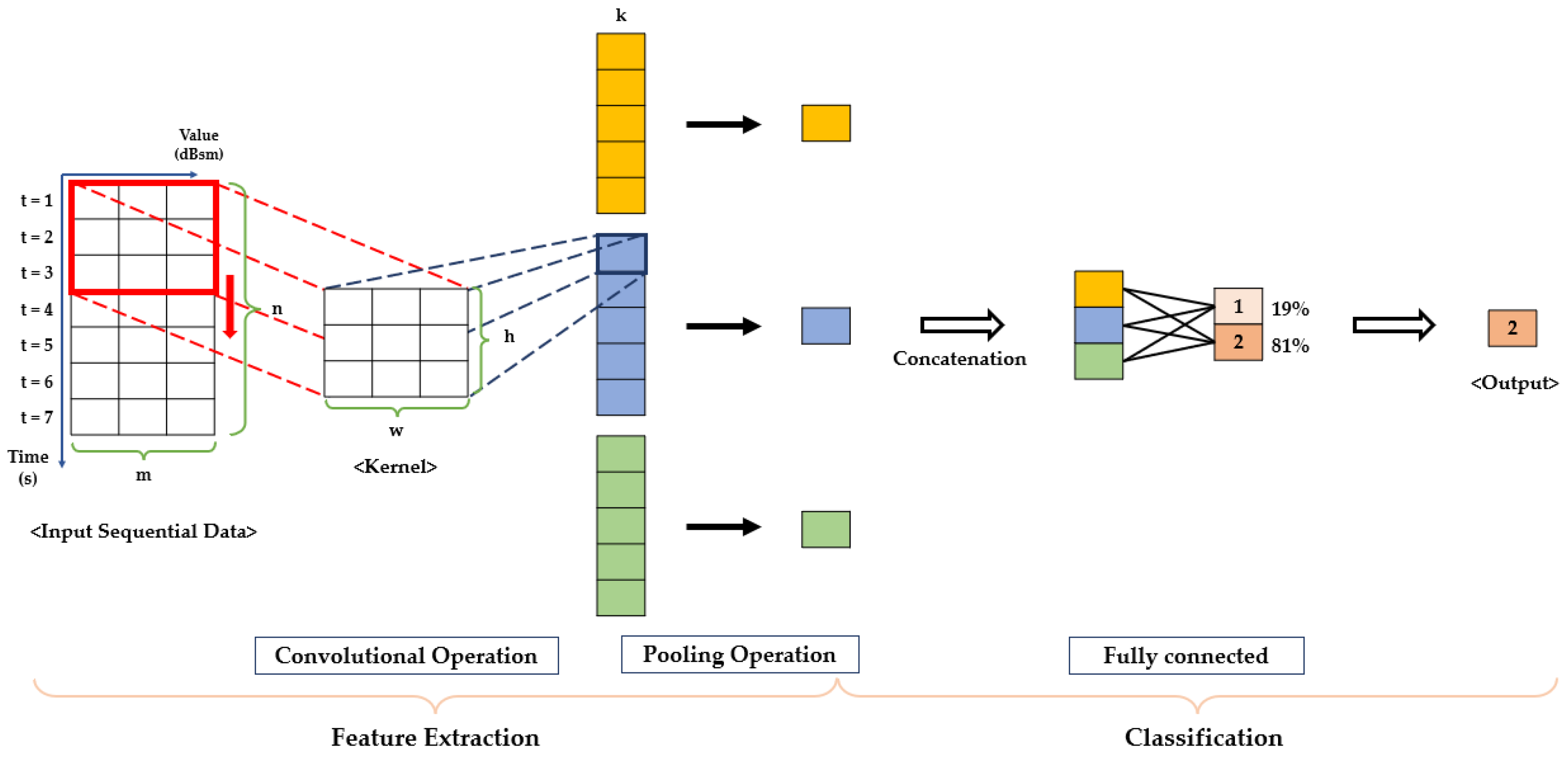
Figure 1 shows the classification with the 3-channel time-series data as inputs using a 1D CNN. It is assumed that there is one CNN layer, and in this case, the number of input dimensions and the width of the kernel should be the same. The meaning of each parameter is as follows: w and h are the width and height of the kernel, k is the number of the kernel, and n and m are the length and channel of input data, respectively.

2.2.2. The GRU

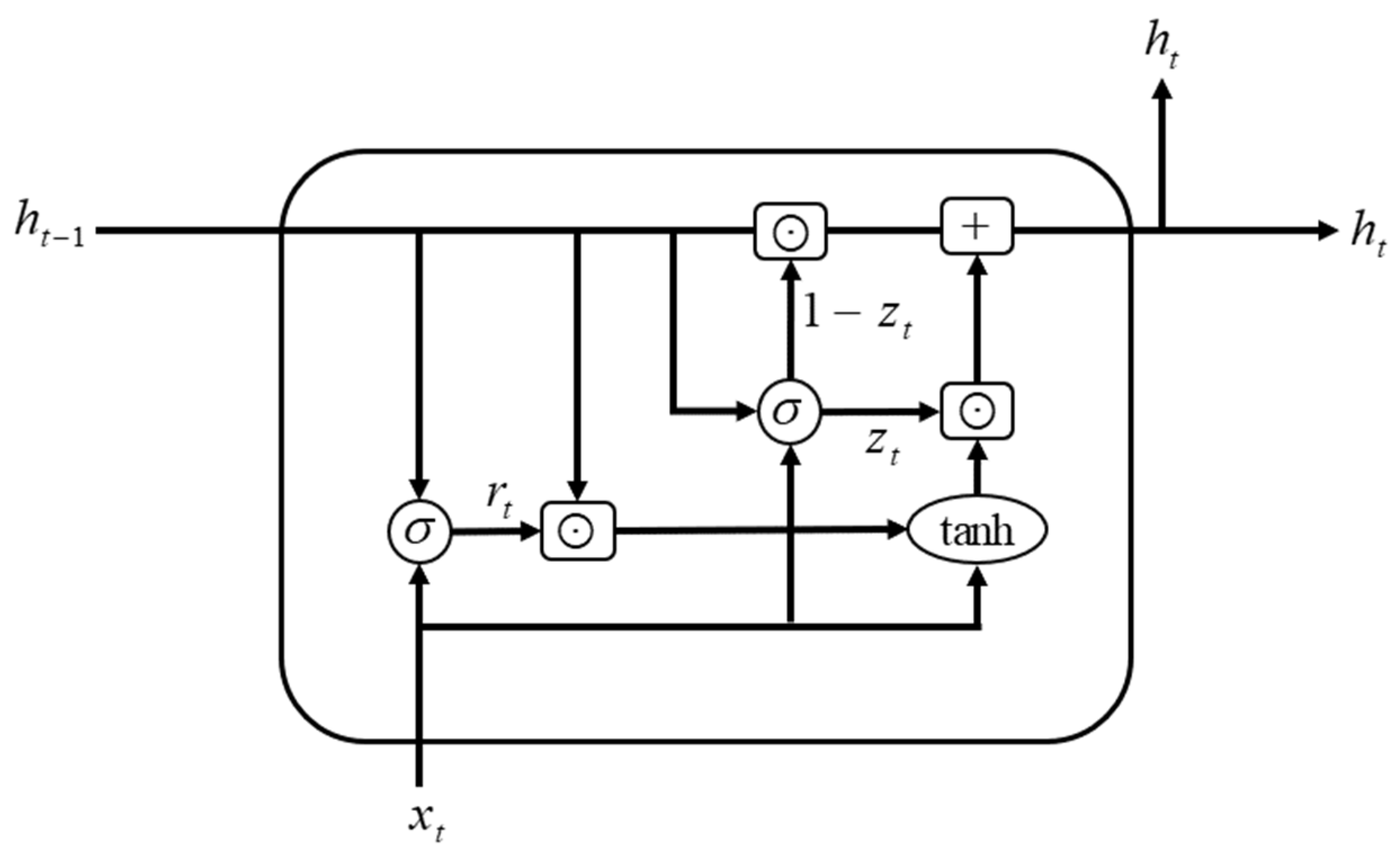
The RNN is one of the artificial neural networks with a cyclic structure and is suitable for processing data in order. However, when the time interval is large, the gradient is lost and the learning ability is greatly reduced. Hochreiter and Schmidhuber solved this problem and proposed the LSTM [37]. The LSTM [38,39] is still widely used in time-series data, and its core idea is that the cell state is connected like a conveyor belt. By applying this, the gradient propagates even if the distance between the states increases. In an LSTM cell, the cell state is controlled through three gates, which are the forget gate, the input gate, and the output gate. In 2014, the GRU [40] was proposed as a network that improved the learning efficiency of the LSTM by modifying the LSTM structure. Unlike the LSTM, the GRU is composed of two gates and has a fast learning speed. In addition, the number of parameters is smaller than that of the LSTM because the cell state and hidden state are integrated into one hidden state. Based on the above, the GRU shows excellent performance for long-term dependencies in time-series data processing and takes less computation time than the LSTM. The structure of the GRU is shown in Figure 2. The GRU is composed of an update gate, that acts as an input gate and the forget gate of the LSTM, and a reset gate that determines the reflection degree of the previous hidden state [41]. GRU equations for determining the hidden state are as follows:
r t = σ ( W r x t + U r h t 1 + b r )
z t = σ ( W z x t + U z h t 1 + b z )
h t = ( 1 z t ) h t 1 + z t tanh ( W h x t + U h ( r t h t 1 ) + b h )
where r t is the reset gate and z t is the update gate at time t . x t is the input value at time t , W and U refer to weights, and b is bias. h t is the hidden state at time t . is the element-wise (Hadamard) multiplication.

3. Experimental Setup

Considering that a real missile flies at a very high speed and hits a target point within a short time, it is necessary to classify the target by using data with a good real-time performance. Therefore, the RCS measurement that ensures that a good real-time performance is selected as the radar data for target classification. In this section, we discuss data generation scenarios and AI data construction. Following this, the parameters to be used when optimizing the 1D CNN–GRU, a network considered for RCS-based target identification, are described.

3.1. Detection Scenario

There are a total of six classification classes, referring to North Korean missiles, and the shape information is shown in Table 1. Flight distances for each class are set as follows: 600 km for Class 1, 300 km for Class 2, 500 km for Class 3, 800 km for Class 4, 500 km for Class 5, and 600 km for Class 6. As shown in Table 1, Class 1 and Class 4, and Class 2 and Class 3 have the same shape but different trajectories. Class 3 and Class 5 have the same trajectory, but different shapes. The reasons for choosing the models in the classes shown in Table 1 are as follows:
  • Confirmation for the classification of missiles with the same shape, but different trajectories;
  • Confirmation for the classification of missiles with the same trajectory, but different shapes;
  • Confirmation for the classification of different types of missiles.
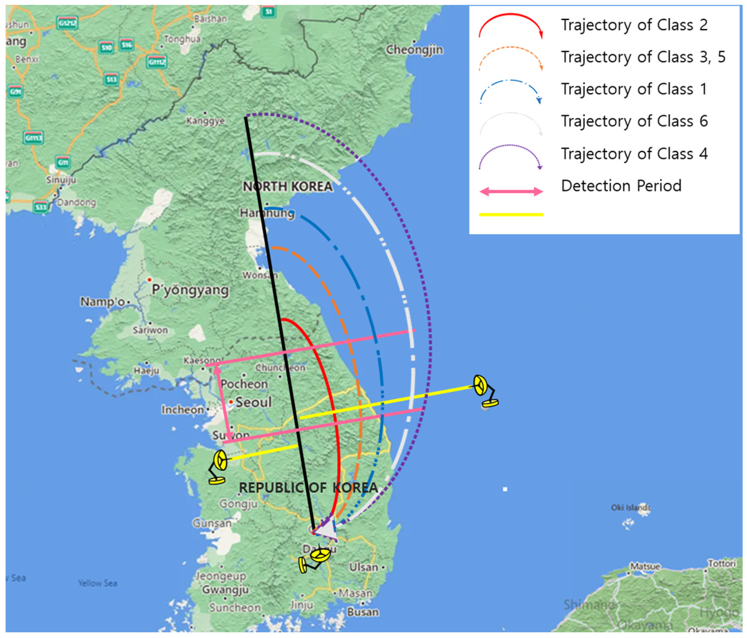
In this paper, we heck the target classification performance after setting the difficult-to-detect environment as above. The detection scenario is shown in Figure 3. We assumed that North Korea is launching a missile and three radars are deployed for detection and classification as shown in this figure. Additionally, the type of radar system was set in mono-static and the yellow line represents the radar line of sight (RLOS). The radar on the right is deployed near the territorial waters of Ulleungdo and its frequency band is 3 GHz— used by the Aegis ship. The radar on the left is deployed in the city of Chungbuk and its frequency band is 1 GHz— used by the ground radar. The radar in the front is at the strike point and its frequency band is 10 GHz. In a low RCS situation, the lower the frequency, the higher the target detection and classification performance. Therefore, the low-frequency band was considered first [42]. The flight trajectory is expressed by each color and line as follows: the solid red line for Class 2, the dashed orange line for Class 3 and 5, the dashed single-dotted blue line for Class 1, the dashed double-dotted light gray line for Class 6, and the dotted purple line of Class 4. The double-headed arrow indicated by the pink line indicates the detection section, which is the mid-phase of the missile flight section. When determining the detection section, after calculating the mid-phase for each of the six missiles, a common mid-phase section was selected. The mid-phase section is mainly used for the detection and identification of missiles because it is possible to detect the target for a long time and be less affected by obstacles in the air.

3.2. DRCS Generation

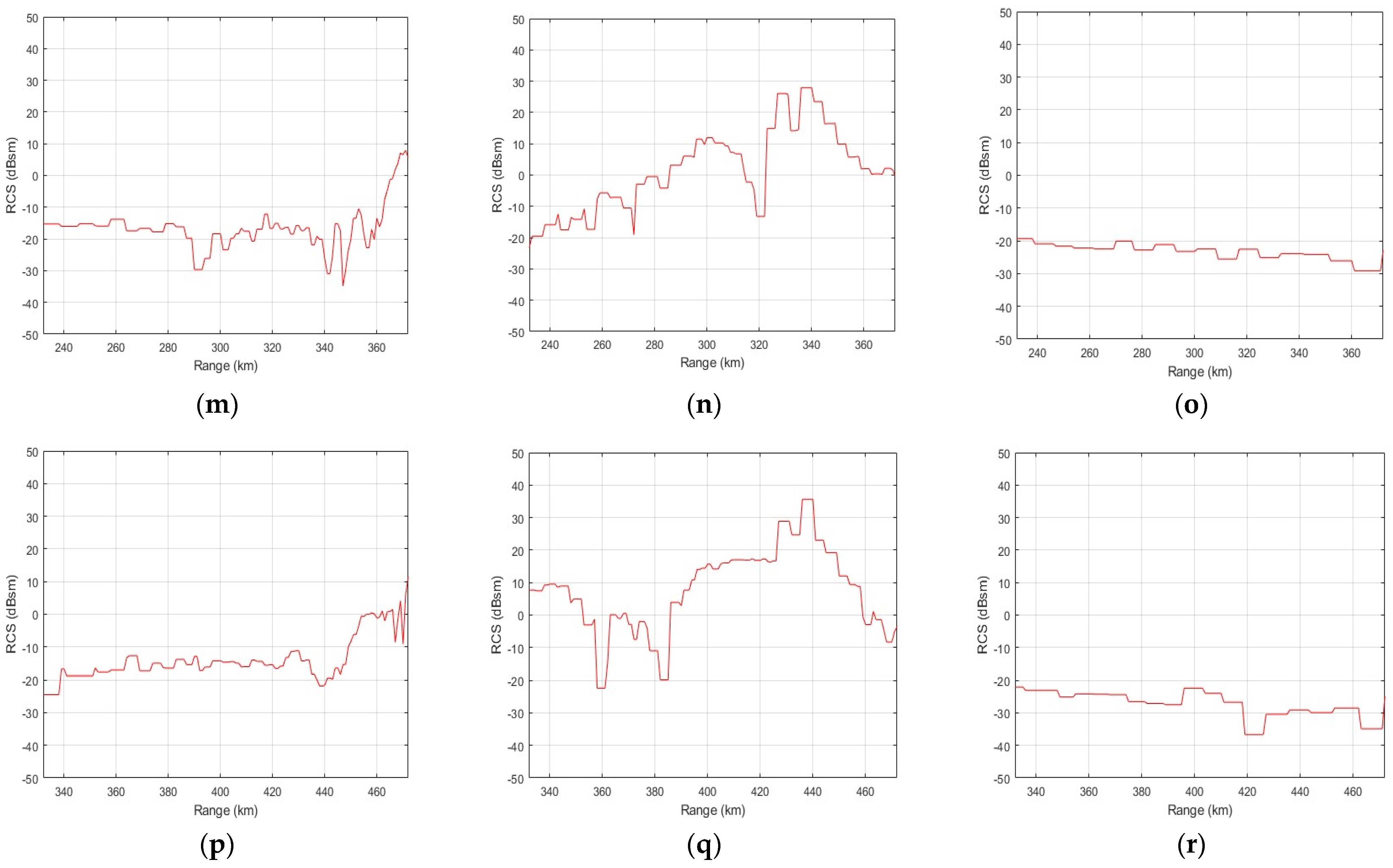
To obtain the RCS measurements of the moving missiles, we generate the dynamic RCS by using the extracted static RCS in advance. The static RCS is a value obtained when the target is not moving and is affected by the shape and material of the target. The dynamic RCS is a value obtained when a target moves along a trajectory and can be extracted by using three types of information such as the static RCS of the target, the trajectory, and the position of the observation radar. Accordingly, even if a missile with the same static RCS value comes in, we obtain different dynamic RCS values depending on the trajectory. The parameters required for static RCS generation have been published previously [43]. A high-frequency structure simulator (HFSS) from Ansys is used to extract static RCS measurements, and a matrix laboratory (MATLAB) is used as a tool to extract dynamic RCS measurements. Before proceeding with classification based on AI, the extracted dynamic RCS measurement is converted as a graph and then quantitatively evaluated to check whether the data can be classified as a target. Figure 4 presents the dynamic RCS graphs, showing the RCS measurement according to the detection period explained in Figure 3. As shown in Figure 4a–c, all missiles extract dynamic RCS measurements of different shapes depending on the frequency band. For Class 2 and Class 3, we confirmed that the dynamic RCS for each is obtained differently at the same frequency, due to their different trajectories, even if the static RCS is the same for each (due to having the same shape and material). We can also expect high classification performance by effectively extracting feature points at all frequencies. As expected, like Figure 4a,d,g,j,m,p, there is a section where all missiles show a similar shape within the same frequency band. However, other shapes are drawn except for sections where similar shapes are visible. This means that even if there is a similar section, it is possible to extract features from other sections, so that classification can be performed. Based on the above results, we predict target classification in complex situations before target classification is possible.

3.3. The Configuration of the Dataset

Having extracted the dynamic RCS measurement through the simulator, as above, the number of data for learning and verification is one and is insufficient for the AI data. Therefore, we need data augmentation for training and testing. First, data preprocessing is performed through normalization. Subsequently, referring to existing papers, the noise level is assumed to be Gaussian noise and data augmentation is performed by Gaussian noise with zero mean and a standard deviation of 0.5 [24]. To set the ratio of the training and the test set to 6:1, respectively, as in the MNIST [44], a total of 36,000 training data sets with 6000 data sets per class, and a total of 6000 test data sets builds 1000 data sets per class. Following this, the Gaussian noise with a zero mean and a standard deviation of 0.9 are added to the test data generated through data augmentation. The reason why the standard deviation of 0.9 was added to the test data is to treat it differently from the learned data.

3.4. The Preparation of Training and Testing Methods for Network Optimization

As time-series prediction models, the LSTM and GRU show good performance when demanding precision from time-series data by maintaining the data trend. However, it has been shown that accuracy deteriorates in data with large fluctuations. Therefore, in this paper, we design a network that can compensate for the weakness of the RCS, which is weak to noise, by combining the GRU, which has strength in time-series data processing, with the 1D CNN, which has strength in feature extraction. The above networks have been, theoretically, analyzed well in the past. Thus, we referred to the mathematical modeling of the 1D CNN [33,34], GRU [38], and LSTM [40]. Following this, we proceeded with the optimization of the 1D CNN–GRU to obtain a model suitable for the RCS because it needs to be tuned according to the data characteristics. Optimization proceeds by experimentally changing the network structure, the hidden unit, and the optimizer, in that order.

3.4.1. The Initial Value for Optimization Network

In the existing study [24], hyperparameters and optimization techniques suitable for networks were analyzed for the AI-based target classification using the RCS measurements. Therefore, in this paper, based on the analysis results of previous studies, the hyperparameters, such as epoch, iteration, and batch size, are set to 30, 50, and 720, respectively. When verifying by experimentally changing the layers of the CNN and GRU in the process of optimizing the network structure, the number of the CNN layers is set to 5 and the number of the GRU layers is set to 3 as initial values. The hidden unit of the GRU layer initially consists of 140-90-30. Additionally, as the number of the GRU layers is changed, the hidden unit consists of 140-90, 140-90-30, and 140-90-60-30. For reference, the initial value of the hidden unit of the GRU layer is set so that the number of nodes can be reduced as it approaches the output layer. Finally, when comparing the classification performance according to the network structure and the hidden unit, the optimization method is set to Adam (adaptive moment), which is commonly used, and the learning rate is selected as 0.001 as suggested in the previous paper [45].

3.4.2. Training and Testing

The network is trained using the previously generated training data. At this time, to increase the reliability of the study, 10 networks are extracted for each case. Following this, the classification performance of the network is checked by extracting three classification results of the learned network based on the verification data. To quantitatively check the classification performance, the accuracy of the confusion matrix is used as an evaluation index [46]. The confusion matrix indicates the degree to which the predicted value agrees with the actual value and is a widely used indicator when evaluating the performance of a network. At this point, the accuracy is a value located on the diagonal of the confusion matrix and indicates how accurately the predicted value matches the actual value. For network performance comparison and analysis, we repeatedly extract the accuracy for each case 30 times and then use the average value as the network accuracy. In addition, the standard deviation is extracted to check the stability of the network performance. In this case, the small standard deviation means that the performance fluctuation range is small.

4. Experiments

4.1. Network Optimization

4.1.1. Structure

The deeper the layer, the more robustly it extracts features, but the amount of computation is also greatly increased, resulting in a longer learning time. On the other hand, if the depth of the layer is too shallow, features cannot be extracted properly and the accuracy is greatly reduced. Therefore, considering the learning efficiency, we experimentally change the number of layers and check the performance. First, by changing the convolutional layer, two structures with high accuracy and low standard deviation are identified and selected. Then, the classification performance is checked by decreasing and increasing the number of the GRU layers in the two selected structures. Through this, the number of layers with high accuracy compared to the amount of computation is determined.
At this point, the number and size of kernels should be set as parameters of the convolutional layer. The kernel size is usually set to an odd number such as 3, 5, or 7. The number of kernels is a parameter that determines the size of the output feature map as the number of nodes in the convolutional layer. As the number of kernels increases, the accuracy improves, but the amount of computation also increases. Therefore, in this paper, the number of kernels is set to increase as the neural network deepens, such as 32, 64, 128, 192, and 256, and the size of the kernel is set to 3, the same as the value set published previously [47].
Table 2 shows the classification accuracy and standard deviation according to the change in the number of convolutional layers of the 1D CNN–GRU set as the initial value. As shown in Table 2, convolutional layer 4—GRU layer 3 (C4G3)—has the highest classification accuracy of 99.31% and the lowest standard deviation of 0.4905. Convolutional layer 5—GRU layer 3 (C5G3)—shows 98.40% accuracy and a low standard deviation of 1.089. With the above two structures, the classification performance according to the change in the number of GRU layers is checked. Table 3 shows the classification results of the 1D CNN–GRU according to the change in the number of GRU layers. As shown in Table 3, the C4G3, which had the best performance in Table 2, has the highest accuracy of 99.31% and the lowest standard deviation of 0.4905. Convolutional layer 5—GRU layer 4 (C5G4)—has the second-best performance as it has an accuracy of 99.12% and a standard deviation of 0.5934.

4.1.2. The Hidden Unit

When the size of the hidden unit is large, the performance is poor and the amount of computation is increased. Therefore, the performance is checked by experimentally changing the configuration of the hidden unit of the GRU layer suitable for the network structure. The network structure uses the two structures with the highest performance in Section 4.1.1.
Table 4 and Table 5 show the classification accuracy and standard deviation according to the change of the hidden unit. As shown in these Tables, the C4G3 and C5G3 have the highest accuracy and lowest standard deviation in the initially set hidden unit configuration despite changing the hidden unit. In addition, the classification accuracy of the C4G3 is 0.19% higher than that of the C5G3 and the standard deviation of the C4G3 is 0.1029 lower than that of the C5G3. As a result, it can be confirmed that the C4G3 network is the most stable and has the highest classification accuracy when its hidden unit is composed of 140-90-30.

4.1.3. Optimization

The optimization algorithm is a technique to find weights and biases to minimize the loss function. The classification performance of networks is compared by changing the optimizer of the network selected in Section 4.1.2. The optimizer considers stochastic gradient descent with momentum (SGDM) [48], root mean square propagation (RMSprop) [49], and Adam by referring to the existing papers [50]. The optimizer selects based on the classification accuracy for accurate target classification.
Table 6 shows the classification results according to the optimizer change of the 1D CNN–GRU. As shown in this table, both Adam and RMSprop have a classification performance of 99.30% or more, and a standard deviation of 0.5532 or less. As described above, the optimizer selects the RMSprop with the highest accuracy based on the classification accuracy. The classification accuracy of the final design of the 1D CNN–GRU is 99.50% and has a standard deviation of 0.5532. The performance of the final design of the 1D CNN–GRU has very high classification accuracy and a low standard deviation.

4.2. The Optimized 1D CNN–GRU

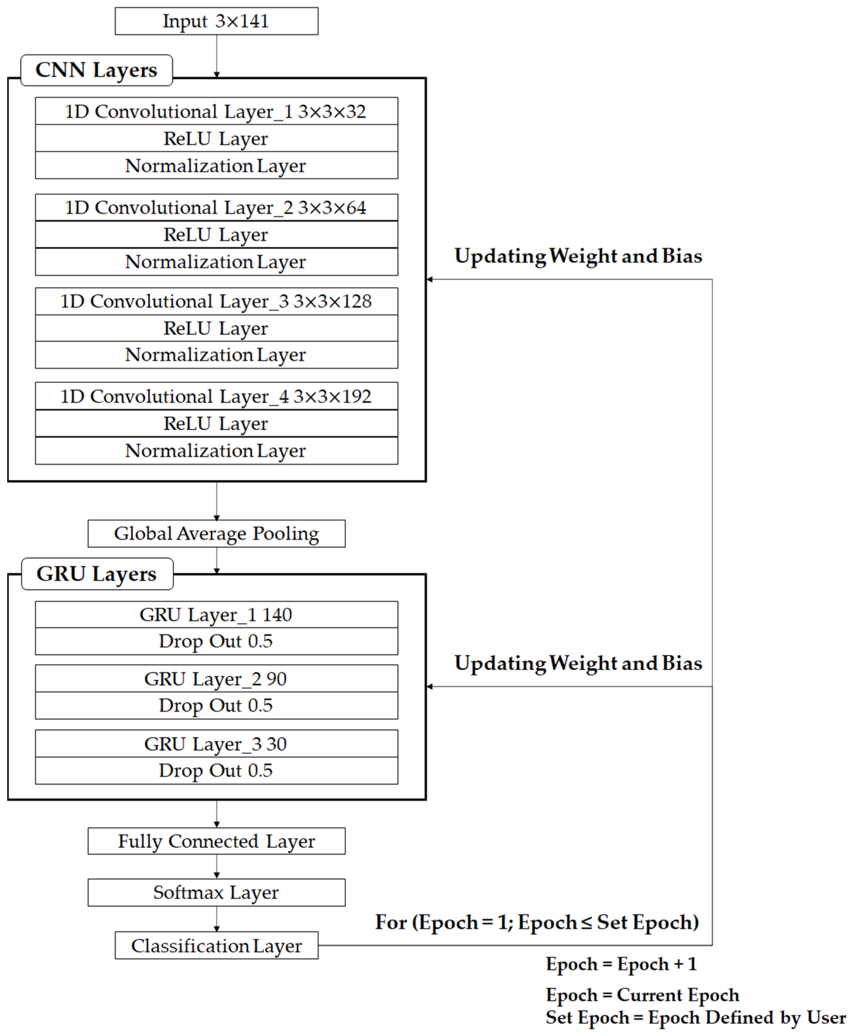
Figure 5 shows the structure and overall flow chart of the final optimization of the 1D CNN–GRU network. The feature extraction is performed by receiving a 3D RCS measurement with a size of 3 × 141 from the CNN as an input. The stride, which is the movement interval of the kernel, is 1, and the causal padding is used to set the output length and input length of the time-series data to be the same in the CNN layer. In addition, to solve the gradient vanishing problem in the CNN layers, the rectified linear unit (ReLU) [51] is used as an activation function and a normalization layer [52] is added. At his point, normalization proceeds with layer normalization. Layer normalization is one of the techniques that came out to solve the problem of batch normalization dependence on batch size. Batch normalization is difficult to use in a time-series data processing model. The reason is that it is difficult to express the entire data when the batch size is small due to the nature of the sequence data. Therefore, in this paper, layer normalization is used to perform normalization in units of layers.
Following this, by extracting the feature map as one value through global average pooling, the number of features is greatly reduced and the features are made into a one-dimensional vector. Subsequently, learning is performed in three GRU layers using a one-dimensional vector. The activation function of the GRU uses the sigmoid and the tanh function. The sigmoid function is used for gate calculation, and the tanh function is used to update the hidden state.
Finally, classification proceeds through the fully connected layer and the softmax layer [53] in the output layer, and the related contents are as follows. The fully connected layer is used to combine features learned from the GRU layer for final classification. At this time, the output size is set to 5, which is equal to the number of missile classes. In addition, since the output form of the GRU layer is in the form of a one-dimensional array, there is no need for a separate flattening operation unlike that used in the 2D CNN. Subsequently, the softmax function is used as an activation function for multi-class classification. The softmax layer performs the softmax function and calculates the probability of the input and outputs the predicted value. At this point, the number of softmax nodes is set as the number of classes to be classified like a fully connected layer, and in this paper, it is set to 5. Finally, the classification layer calculates the difference between the predicted value and the actual value through a loss function and updates the parameters (weight and bias) of the network. The loss function is generally set to cross-entropy, which is used in classification problems.

5. Experimental Results

5.1. The Comparison of Classification Results of Optimized Networks

To compare and analyze network performance, the 1D CNN and 1D CNN–LSTM are selected as comparison groups, and the classification accuracy, standard deviation, total number of parameters, and algorithm operation time of the three networks are checked. In addition, five classes are selected to check if a good performance is seen in the other RCS measurements. The DRCS generation and data composition method for the additional five classes is the same as mentioned in Section 3, and thus, the learning and verification data are established. Using the three trained networks, the classification accuracy, standard deviation, and algorithm operation time are checked, and the comparison and analysis are performed with the network designed in Section 4.
Table 7 and Table 8 are the results of comparing the classification performance of three networks trained with the DRCS dataset generated in Section 3 and the additionally selected DRCS dataset. Here, Table 7 shows the classification results for six classes using the data from the network optimization in Section 4, and Table 8 shows the classification results for the five newly added classes. As shown in these Tables, a high classification accuracy of 98.93% or more can be confirmed in all networks, and the 1D CNN–GRU has the highest accuracy. The running time of the algorithms is shown in Table 7 and Table 8. This running time represents the time taken to process one sequence of data. The simulation computer specifications used in this paper are as follows: AMD Ryzen 7 5800X, 32 GB RAM, and NVIDIA GeForce RTX 3090. Although the network structure of the proposed method is complex, it was confirmed that the operating time was not significantly different from that of the conventional methods. However, the difference in performance could be confirmed. Through this result, it is expected that real-time classification is possible for all three networks. In addition, as shown in the respective Tables, the performance of the 1D CNN–GRU has an accuracy difference of 0.1%, so the difference is not large and is within the standard deviation. This means that if the network designed in this paper is used for target classification using the RCS measurements, it could generally have a high classification performance as shown in the table below.
In the table below, the 1D CNN has a lower accuracy than the 1D CNN–GRU, but it has a small standard deviation, so it may be difficult to select a network. Therefore, in the next section, we plan to check the network that could be used by compensating for the weakness in noise, which is a disadvantage of the RCS, by comparing and analyzing the performance of the networks by increasing the noise level.

5.2. The Classification Results According to the Noise Level

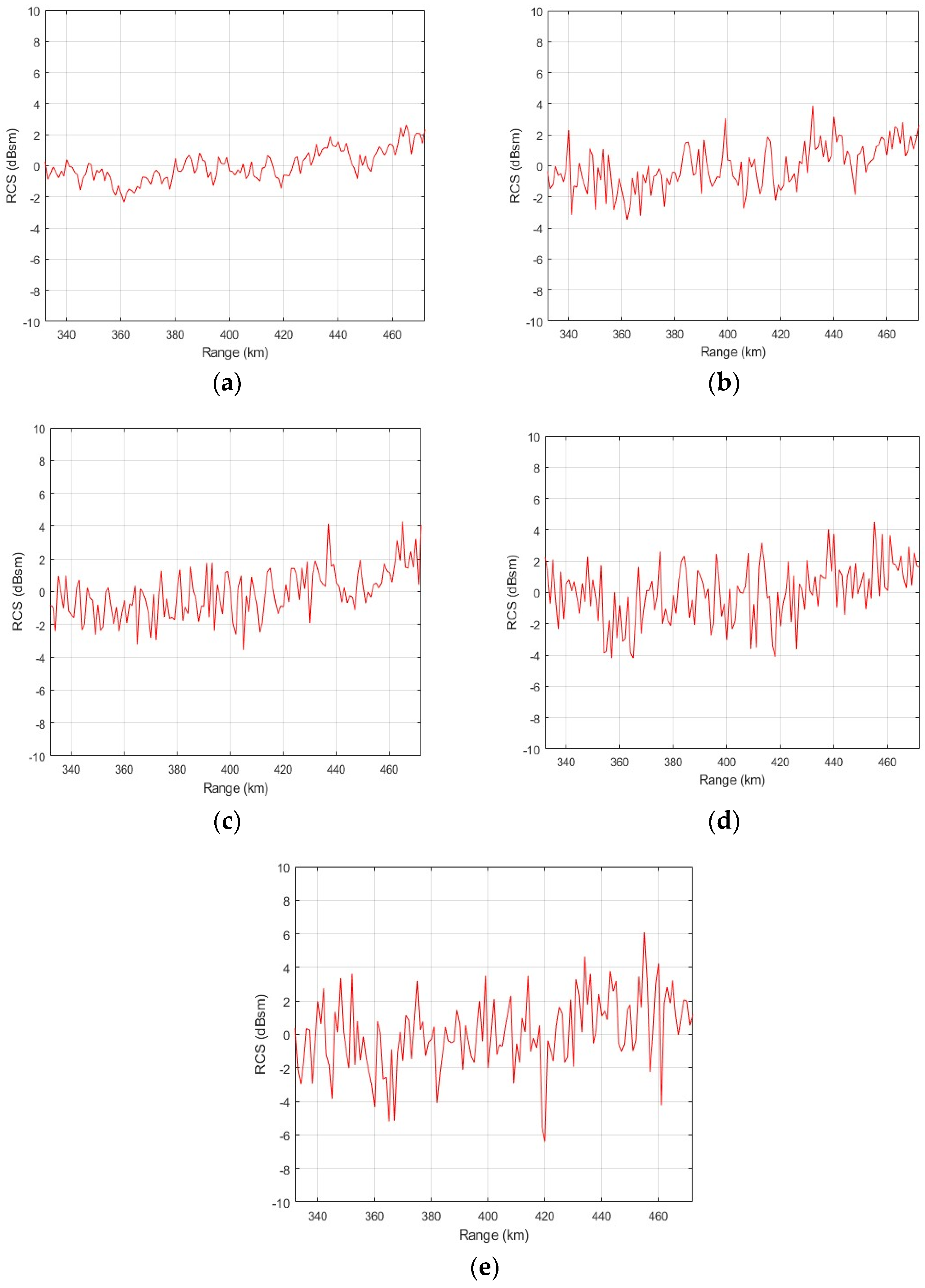
To check the classification performance according to the noise influence of the networks, the classification performance of two different datasets is checked by increasing the noise level. The noise type is assumed to be Gaussian noise and its standard deviation is increased by 0.3 based on the zero mean and the standard deviation of 0.9. Figure 6 shows the change in the dynamic RCS graph according to the standard deviation of Gaussian noise using the class 1 training data generated in Section 3. Figure 6a indicates a dynamic RCS graph of class 1 used for learning, and Figure 6b–e show dynamic RCS graphs when the standard deviation is augmented by 0.3. As shown in Figure 6, the deformation of the graph increases as the noise level increases.
In Figure 7, the average accuracy according to the noise level change for three networks is compared. Figure 7a shows the change in the classification performance of networks according to the noise level of the data used for optimization with six classes. Figure 7b shows the change in the classification performance of networks according to the noise level of the new data with the five newly added classes. In Figure 7, the 1D CNN, 1D CNN–LSTM, and 1D CNN–GRU are represented by red dashed lines, blue solid lines, and black dash-dotted lines, respectively. At a standard deviation of 0.9, all networks show excellent performance, and the 1D CNN and 1D CNN–GRU have a slightly higher performance than the 1D CNN–LSTM. However, the 1D CNN–LSTM and 1D CNN–GRU show a higher classification performance than the 1D CNN with a standard deviation of 1.5 in Figure 7a and 1.0 in Figure 7b. Consequently, the 1D CNN–LSTM and 1D CNN–GRU, which are combined networks, are stronger in noise than the 1D CNN. In addition, it is confirmed that the 1D CNN–GRU designed in this paper is the most robust to noise among the networks in both datasets. Therefore, it is desirable to use the 1D CNN–GRU for the RCS-based target classification because the 1D CNN–GRU designed in this paper can compensate for the weakness of noise, which is the disadvantage of the RCS.

6. Conclusions

After selecting radar data and networks to improve real-time target classification performance using surface-to-air radar, we designed the network and confirmed the classification performance. In addition, we considered the 1D CNN and 1D CNN–LSTM as comparison groups to confirm the designed network classification performance.
For real-time multiclass classification, the RCS, a radar measurement, was selected as input data. Although the RCS is capable of real-time acquisition, it has the disadvantage of being vulnerable to noise. To compensate for the shortcomings of the RCS, the 1D CNN–GRU, a combined network, was considered by adding a GRU layer for the more effective processing of time-series data to the 1D CNN with strong feature extraction strength. We designed a 1D CNN–GRU that has four convolutional layers and three GRU layers to fit the DRCS data characteristics. In the present study, the GRU hidden units consisted of 140, 90, and 30, and RMSprop as the optimizer was used. The designed network had the highest accuracy of 99.50%, confirming the best classification performance. In addition, with the network designed in this paper, the performance was checked as to whether target classification is possible for other RCS measurements. As a result of checking the classification performance based on the newly generated data set, the 1D CNN–GRU had the highest accuracy of 99.40%.
To select a network that could compensate for the weakness of the RCS, the noise was increased to check the classification performance according to the noise of the networks. We tested the existing data set and the new data set. At a low level of noise, the 1D CNN and the 1D CNN–GRU had slightly higher accuracies than the 1D CNN–LSTM, but the performance of all networks was high at a 98.93% accuracy. However, as the high level of noise was added, the accuracy of the combined networks of the 1D CNN–LSTM and 1D CNN–GRU was higher than that of the 1D CNN, with a standard deviation of 1.5 when using the existing data set and 1.0 when using the new data set. In addition, it was confirmed that the 1D CNN–GRU had the highest accuracy value at all noise levels in the two data sets. Based on the above results, it can be seen that the combined network is stronger in noise than the general network. Therefore, it was confirmed that the 1D CNN–GRU designed in this paper is suitable for RCS-based target classification by supplementing the shortcomings of the RCS.
By optimizing and designing, we proposed a 1D CNN–GRU that is less affected by noise and has high classification performance and learning efficiency. Furthermore, when the test was conducted by changing the type of missile, we confirmed a higher performance than other networks. As a result, we expect to enable an accurate and rapid preemptive response in the missile defense system by using the proposed network. In the future, our researchers will conduct a study to improve target classification performance after constructing various scenarios, including situations such as a low RCS and various different trajectories, such as pull-up maneuvers.
Author Contributions

Conceptualization, A.R.K., H.S.K., C.H.K. and S.Y.K.; methodology, A.R.K., H.S.K., C.H.K. and S.Y.K.; validation, A.R.K., H.S.K., C.H.K. and S.Y.K.; formal analysis, A.R.K., H.S.K., C.H.K. and S.Y.K.; investigation, A.R.K. and H.S.K.; data curation, A.R.K. and H.S.K.; writing—original draft preparation, A.R.K., H.S.K., C.H.K. and S.Y.K.; writing—review and editing, C.H.K. and S.Y.K.; visualization, A.R.K. and H.S.K.; supervision, C.H.K. and S.Y.K.; funding acquisition, C.H.K. and S.Y.K. All authors have read and agreed to the published version of the manuscript.

Funding

This research received no external funding.

Data Availability Statement

Not applicable.

Acknowledgments

This research was supported by the National Research Foundation of Republic of Korea (NRF) grant funded by the Ministry of Science and ICT, the Republic of Korea (No. 2021R1C1C1009219, 2021R1F1A1063298).

Conflicts of Interest

The authors declare no conflict of interest.

References

  1. Galán, J.J.; Carrasco, R.A.; LaTorre, A. Military Applications of Machine Learning: A Bibliometric Perspective. Mathematics 2022, 10, 1397. [Google Scholar] [CrossRef]
  2. Wang, W.; Liu, H.; Lin, W.; Chen, Y.; Yang, J.A. Investigation on Works and Military Applications of Artificial Intelligence. IEEE Access 2020, 8, 131614–131625. [Google Scholar] [CrossRef]
  3. Kim, H.S.; Kim, A.R.; Kang, C.H.; Kim, S.Y. Radar Measurement Analysis for Improving Target Detection and Identification. J. ICROS 2022, 28, 391–396. [Google Scholar] [CrossRef]
  4. Sehgal, B.; Shekhawat, H.S.; Jana, S.K. Automatic Radar Target Identification Using Radar Cross Section Fluctuations and Recurrent Neural Networks. In Proceedings of the TENCON 2019–2019 IEEE Region 10 Conference (TENCON), Kochi, India, 17–20 October 2019; pp. 2490–2495. [Google Scholar]
  5. Kim, H.S.; Kim, A.R.; Kang, C.H.; Kim, S.Y. Similarity Test of Missile according to Detection Distance Interval Considering Noise Level. In Proceedings of the ICROS 2022, Geoje, Korea, 22–24 June 2021; pp. 566–567. [Google Scholar]
  6. Persico, A.R.; Clemente, C.; Gaglione, D.; Ilioudis, C.V.; Cao, J.; Pallotta, L.; De Maio, A.; Proudler, I.K.; Soraghan, J.J. On Model, Algorithms, and Experiment for Micro-Doppler-Based Recognition of Ballistic Targets. IEEE Trans. Aerosp. Electron. Syst. 2017, 53, 1088–1108. [Google Scholar] [CrossRef] [Green Version]
  7. Choi, I.O.; Park, S.H.; Kim, S.H.; Lee, S.H.; Kim, K.T. Estimation of the Micro-Motion Parameters of a Missile Warhead Using a Micro-Doppler Profile. In Proceedings of the 2016 IEEE Radar Conference (RadarConf), Philadelphia, PA, USA, 2–6 May 2016; pp. 1–5. [Google Scholar]
  8. Persico, A.R.; Clemente, C.; Pallotta, L.; De Maio, A.; Soraghan, J. Micro-Doppler Classification of Ballistic Threats Using Krawtchouk Moments. In Proceedings of the 2016 IEEE Radar Conference (RadarConf), Philadelphia, PA, USA, 2–6 May 2016; pp. 1–6. [Google Scholar]
  9. Sun, H.-X.; Liu, Z. Micro-Doppler Feature Extraction for Ballistic Missile Warhead. In Proceedings of the 2008 International Conference on Information and Automation, Changsha, China, 20–23 June 2008; IEEE: New York, NY, USA, 2008; pp. 1333–1336. [Google Scholar]
  10. Parvatha, R.S.; Ramya, T.; Aparanji, G.S.; Mamtha, M.V.; Gupta, A.; Tom, R.J. Signature Based Radar Target Classification. In Proceedings of the 2021 International Conference on Recent Trends on Electronics, Information, Communication and Technology (RTEICT), Bangalore, India, 27–28 August 2021; pp. 873–879. [Google Scholar]
  11. Chen, L.; Chen, R. A New Radar Target Recognition Method Based on Complex High Resolution Range Profiles. In Proceedings of the International Conference on Microwave and Millimeter Wave Technology (ICMMT), Shenzhen, China, 5–8 May 2012; pp. 1–4. [Google Scholar]
  12. Yuan, Y.X.; Luo, Y.; Ni, J.C.; Zhang, Q. Inverse Synthetic Aperture Radar Imaging Using an Attention Generative Adversarial Network. Remote Sens. 2022, 14, 3509. [Google Scholar] [CrossRef]
  13. Wei, S.; Liang, J.; Wang, M.; Zeng, X.; Shi, J.; Zhang, X. CIST: An Improved ISAR Imaging Method Using Convolution Neural Network. Remote Sens. 2020, 12, 2641. [Google Scholar] [CrossRef]
  14. Li-hua, L.; Zhuang, W.; Wei-dong, H. Precession Period Extraction of Ballistic Missile Based on Radar Measurement. In Proceedings of the 2006 CIE International Conference on Radar, Shanghai, China, 16–19 October 2006; pp. 1–4. [Google Scholar]
  15. Feng, B.; Chen, B.; Liu, H.W. Radar HRRP Target Recognition with Deep Networks. Pattern Recognit. 2017, 61, 379–393. [Google Scholar] [CrossRef]
  16. Chen, J.; Xu, S.; Chen, Z. Convolutional Neural Network for Classifying Space Target of the Same Shape by Using RCS Time series. IET Radar Sonar Navig. 2018, 12, 1268–1275. [Google Scholar] [CrossRef]
  17. Yao, X.; Shi, X.; Zhou, F. Human Activities Classification Based on Complex-Value Convolutional Neural Network. IEEE Sens. J. 2020, 20, 7169–7180. [Google Scholar] [CrossRef]
  18. Mansukhani, J.; Penchalaiah, D.; Bhattacharyya, A. RCS Based Target Classification Using Deep Learning Methods. In Proceedings of the 2021 2nd International Conference on Range Technology (ICORT), Chandipur, Balasore, India, 5–6 August 2021; pp. 1–5. [Google Scholar]
  19. Fu, R.; Al-Absi, M.A.; Kim, K.H.; Lee, Y.S.; Al-Absi, A.A.; Lee, H.J. Deep Learning-Based Drone Classification Using Radar Cross Section Signatures at mmWave Frequencies. IEEE Access 2021, 9, 161431–161444. [Google Scholar] [CrossRef]
  20. Jithesh, V.; Sagayaraj, M.J.; Srinivasa, K.G. LSTM Recurrent Neural Networks for High Resolution Range Profile Based Radar Target Classification. In Proceedings of the 2017 3rd International Conference on Computational Intelligence and Communication Technology (CICT), Ghaziabad, India, 9–10 February 2017; pp. 1–6. [Google Scholar]
  21. Lu, W.; Zhang, Y.; Xu, C.; Lin, C.; Huo, Y. A Deep Learning-Based Satellite Target Recognition Method Using Radar Data. Sensors 2019, 19, 2008. [Google Scholar] [CrossRef] [PubMed] [Green Version]
  22. Zeng, K.; Zhuang, X.; Xie, Y.; Xi, Z. Hypersonic Vehicle Trajectory Classification Using Improved CNN-LSTM Model. In Proceedings of the 2021 IEEE International Conference on Unmanned Systems (ICUS), Beijing, China, 26–28 October 2021; pp. 691–696. [Google Scholar]
  23. Liu, H.; Ma, R.; Li, D.; Yan, L.; Ma, Z. Machinery Fault Diagnosis Based on Deep Learning for Time Series Analysis and Knowledge Graphs. J. Signal. Process. Syst. 2021, 93, 1433–1455. [Google Scholar] [CrossRef]
  24. Kim, A.R.; Kim, H.S.; Kang, C.H.; Kim, S.Y. Classification of Missiles by Optimized 1D-CNN Using Radar Data. In Proceedings of the 2022 22nd International Conference on Control, Automation and Systems (ICCAS), Busan, Korea, 27 November–1 December 2022. [Google Scholar]
  25. Dybdal, R.B. Radar Cross Section Measurements. IEEE Trans. Antennas Propag. 1987, 75, 498–516. [Google Scholar] [CrossRef]
  26. Knott, E.; Schaeffer, J.; Tulley, M. Radar Cross Section; SciTech Publishing: New York, NY, USA, 2004. [Google Scholar]
  27. LeCun, Y.; Boser, B.; Denker, J.S.; Henderson, D.; Howard, R.E.; Hubbard, W.; Jackel, L.D. Backpropagation Applied to HandWritten Zip Code Recognition. Neural Comput. 1989, 1, 541–551. [Google Scholar] [CrossRef]
  28. Qi, K.; Guan, Q.; Yang, C.; Peng, F.; Shen, S.; Wu, H. Concentric Circle Pooling in Deep Convolutional Networks for Remote Sensing Scene Classification. Remote Sens. 2018, 10, 934. [Google Scholar] [CrossRef] [Green Version]
  29. Zeiler, M.D.; Fergus, R. Stochastic Pooling for Regularization of Deep Convolutional Neural Networks. arXiv 2013, arXiv:1301.3557. [Google Scholar]
  30. Zhang, J.; Zhang, M.; Shi, L.; Yan, W.; Pan, B. A Multi-Scale Approach for Remote Sensing Scene Classification Based on Feature Maps Selection and Region Representation. Remote Sens. 2019, 11, 2504. [Google Scholar] [CrossRef] [Green Version]
  31. Haq, A.U.; Li, J.P.; Ahmad, S.; Khan, S.; Alshara, M.A.; Alotaibi, R.M. Diagnostic Approach for Accurate Diagnosis of COVID-19 Employing Deep Learning and Transfer Learning Techniques Through Chest X-ray Images Clinical Data in E-healthcare. Sensors 2021, 21, 8219. [Google Scholar] [CrossRef]
  32. Wen, L.; Li, X.; Gao, L.; Zhang, Y. A New Convolutional Neural Network Based Data-Driven Fault Diagnosis Method. IEEE Trans. Ind. Electron. 2018, 65, 5990–5998. [Google Scholar] [CrossRef]
  33. Kiranyaz, S.; Ince, T.; Hamila, R.; Gabbouj, M. Convolutional Neural Networks for Patient-Specific ECG Classification. In Proceedings of the 2015 37th Annual International Conference of the IEEE Engineering in Medicine and Biology Society (EMBC), Milan, Italy, 25–29 August 2015; pp. 2608–2611. [Google Scholar]
  34. Chen, Y. Convolutional Neural Network for Sentence Classification. Master’s Thesis, University of Waterloo, Waterloo, ON, Canada, 2015. [Google Scholar]
  35. Wang, H.; Liu, Z.; Liu, Z.; Qin, Y. Understanding and Learning Discriminant Features Based on Multiattention 1DCNN for Wheelset Bearing Fault Diagnosis. IEEE Trans. Ind. Inform. 2019, 16, 5735–5745. [Google Scholar] [CrossRef]
  36. Eren, L.; Ince, T.; Kiranyaz, S. A Generic Intelligent Bearing Fault Diagnosis System Using Compact Adaptive 1D CNN Classifier. J. Signal. Process. Syst. 2018, 91, 179–189. [Google Scholar] [CrossRef]
  37. Hochreiter, S.; Schmidhuber, J.J. Long Short-Term Memory. Neural Comput. 1997, 9, 1–32. [Google Scholar] [CrossRef]
  38. Kłosowski, G.; Rymarczyk, T.; Wójcik, D.; Skowron, S.; Cieplak, T.; Adamkiewicz, P. The Use of Time-Frequency Moments as Inputs of LSTM Network for ecg Signal Classification. Electronics 2020, 9, 1452. [Google Scholar] [CrossRef]
  39. Harfiya, L.N.; Chang, C.C.; Li, Y.H. Continuous Blood Pressure Estimation Using Exclusively Photopletysmography by LSTM-Based Signal-to-Signal Translation. Sensors 2021, 21, 2952. [Google Scholar] [CrossRef] [PubMed]
  40. Cho, K.; Van Merriënboer, B.; Gulcehre, C.; Bahdanau, D.; Bougares, F.; Schwenk, H.; Bengio, Y. Learning Phrase Representations Using RNN Encoder-Decoder for Statistical Machine Translation. arXiv 2014, arXiv:1406.1078. [Google Scholar]
  41. Althelaya, K.A.; El-Alfy, E.S.M.; Mohammed, S. Stock Market Forecast Using Multivariate Analysis with Bidirectional and Stacked (LSTM, GRU). In Proceedings of the 2018 21st Saudi Computer Society National Computer Conference (NCC), Riyadh, Saudi Arabia, 25–26 April 2018; pp. 1–7. [Google Scholar]
  42. Zohuri, B. Radar Energy Warfare and the Challenges of Stealth Technology; Springer International Publishing: Berlin, Germany, 2020. [Google Scholar]
  43. Kim, H.S.; Kim, A.R.; Kang, C.H.; Kim, S.Y. Extraction of Dynamic Radar Cross Section Measurement Based on High Frequency Structure Simulator. In Proceedings of the Society of Aerospace System Engineering (SASE) 2022 Spring Conference, Juju, Republic of Korea, 18–21 May 2021. [Google Scholar]
  44. Xiao, H.; Rasul, K.; Vollgraf, R. Fashion-MNIST: A Novel Image Dataset for Benchmarking Machine Learning Algorithms. arXiv 2017, arXiv:1708.07747. [Google Scholar]
  45. Duchi, J.; Hazan, E.; Singer, Y. Adaptive Subgradient Methods for Online Learning and Stochastic Optimization. J. Mach. Learn. Res. 2011, 12, 2121–2159. [Google Scholar]
  46. Grandini, M.; Bagli, E.; Visani, G. Metrics for Multi-Class Classification: An Overview. arXiv 2020, arXiv:2008.05756. [Google Scholar]
  47. Kiranyaz, S.; Avci, O.; Abdeljaber, O.; Ince, T.; Gabbouj, M.; Inman, D.J. 1D Convolutional Neural Networks and Applications: A Survey. arXiv 2019, arXiv:1905.03554. [Google Scholar] [CrossRef]
  48. Rumenlhart, D.E.; McClelland, J.L. Parallel Distributed Processing; Explorations in the Microstructure of Cognition: Foundations; MIT Press: Cambridge, MA, USA, 1986; Volume 1. [Google Scholar]
  49. Tieleman, T.; Hinton, G. Lecture 6.5—RmsProp: Divide the Gradient by a Running Average of Its Recent Magnitude. 2012. Available online: https://www.youtube.com/watch?v=defQQqkXEfE (accessed on 7 August 2021).
  50. Lin, J.; Li, H.; Liu, N.; Gao, J.; Li, Z. Automatic Lithology Identification by Applying LSTM to Logging Data: A Case Study in X Tight Rock Reservoirs. IEEE Geosci. Remote. Sens. Lett. 2021, 18, 1361–1365. [Google Scholar] [CrossRef]
  51. Nair, V.; Hinton, G. Rectified Linear Units Improve Restricted Boltzmann Machines. In Proceedings of the 27th International Conference on Machine Learning (ICML-10), Haifa, Israel, 21–24 June 2010; pp. 807–814. [Google Scholar]
  52. Ba, J.; Kiros, J.; Hinton, G. Layer Normalization. arXiv 2016, arXiv:1607.06450. [Google Scholar]
  53. Lecun, Y.; Bottou, L.; Bengio, Y.; Haffner, P. Gradient-Based Learning Applied to Document Recognition. Proc. IEEE 1998, 86, 2278–2324. [Google Scholar] [CrossRef]
Figure 1. The architecture of the 1D CNN for classification.
Remotesensing 15 00577 g001
Figure 2. The architecture of the GRU.
Remotesensing 15 00577 g002
Figure 3. The detection scenario.
Remotesensing 15 00577 g003
Figure 4. The original dynamic RCS graph according to the frequency for classes 1–6: (a) 1 GHz of class 1; (b) 3 GHz of class 1; (c) 10 GHz of class 1; (d) 1 GHz of class 2; (e) 3 GHz of class 2; (f) 10 GHz of class 2; (g) 1 GHz of class 3; (h) 3 GHz of class 3; (i) 10 GHz of class 3; (j) 1 GHz of class 4; (k) 3 GHz of class 4; (l) 10 GHz of class 4; (m) 1 GHz of class 5; (n) 3 GHz of class 5; (o) 10 GHz of class 5; (p) 1 GHz of class 6; (q) 3 GHz of class 6; (r) 10 GHz of class 6.
Remotesensing 15 00577 g004aRemotesensing 15 00577 g004b
Figure 5. The architecture of the optimized 1D CNN–GRU for the RCS measurement classification.
Remotesensing 15 00577 g005
Figure 6. The dynamic RCS graphs according to the standard deviation of Gaussian noise added in class 1 dataset: (a) standard deviation of 0.5; (b) standard deviation of 0.9; (c) standard deviation of 1.2; (d) standard deviation of 1.5; (e) standard deviation of 1.8.
Remotesensing 15 00577 g006
Figure 7. The average accuracy according to the standard deviation of Gaussian noise in the optimized networks: (a) using this paper’s dataset; (b) using a new dataset.
Remotesensing 15 00577 g007
Table 1. Information on the shape, size, and trajectory of missiles.
Number of ClassShapeSize (L × D)Trajectory
1Remotesensing 15 00577 i00115.5 × 1.3Remotesensing 15 00577 i002
2Remotesensing 15 00577 i00311.25 × 0.88Remotesensing 15 00577 i004
3Remotesensing 15 00577 i00511.25 × 0.88Remotesensing 15 00577 i006
4Remotesensing 15 00577 i00715.5 × 1.3Remotesensing 15 00577 i008
5Remotesensing 15 00577 i0097.5 × 0.95Remotesensing 15 00577 i010
6Remotesensing 15 00577 i01110.1 × 1.26Remotesensing 15 00577 i012
Table 2. The classification results according to changes in the number of convolutional layers of the 1D CNN–GRU.
Layer Structure *Average Accuracy (%)Standard Deviation
C3G397.50902.9906
C4G399.30900.4905
C5G398.40401.0890
C6G396.09303.2094
* C represents the convolutional layer and G represents the GRU layer.
Table 3. The classification results according to changes in the number of GRU layers of the 1D CNN–GRU.
Layer Structure *Average Accuracy (%)Standard Deviation
C4G299.10900.7500
C4G399.30900.4905
C4G498.67000.7674
C5G297.87101.8970
C5G398.40401.0890
C5G499.11500.5934
* C represents the convolutional layer and G represents the GRU layer.
Table 4. The classification results according to changes in hidden units of the 1D CNN–GRU with the C4G3 * structure.
Configuration of Hidden UnitAverage Accuracy (%)Standard Deviation
100-90-3098.38700.9573
100-90-6098.55400.9548
140-90-3099.30900.4905
140-90-6097.98001.7712
* C represents the convolutional layer and G represents the GRU layer.
Table 5. The classification results according to changes in hidden units of the 1D CNN–GRU with the C5G4 * structure.
Configuration of Hidden UnitAverage Accuracy (%)Standard Deviation
100-90-60-3098.67601.0824
100-90-60-6098.23001.4758
140-90-60-3099.11500.5934
140-90-60-6098.69300.6826
* C represents the convolutional layer and G represents the GRU layer.
Table 6. The classification results according to changes in the optimizer of the 1D CNN–GRU with the C4G3 * structure and 140-90-30 hidden units.
OptimizerAverage Accuracy (%)Standard Deviation
Adam99.30900.4905
RMSprop99.50300.5532
SGDM98.80101.1380
* C represents the convolutional layer and G represents the GRU layer.
Table 7. The classification results of the optimized 1D CNN-based networks using this paper’s dataset.
1D CNN1D CNN–LSTM1D CNN–GRU
Total Parameters (kilo)255.7480.4319.2
Average Accuracy (%)99.431099.124099.5030
Standard Deviation0.46600.73740.5532
Running Time (s)0.00020720.00025940.0002608
Table 8. The classification results of the optimized 1D CNN-based networks using the new dataset.
1D CNN1D CNN–LSTM1D CNN–GRU
Average Accuracy (%)99.326798.931199.3978
Standard Deviation0.28201.33560.8490
Running Time (s)0.00020620.00023420.0002368
Disclaimer/Publisher’s Note: The statements, opinions and data contained in all publications are solely those of the individual author(s) and contributor(s) and not of MDPI and/or the editor(s). MDPI and/or the editor(s) disclaim responsibility for any injury to people or property resulting from any ideas, methods, instructions or products referred to in the content.