Ensemble Machine Learning for Mapping Tree Species Alpha-Diversity Using Multi-Source Satellite Data in an Ecuadorian Seasonally Dry Forest

Abstract

The increased variety of satellite remote sensing platforms creates opportunities for estimating tropical forest diversity needed for environmental decision-making. As little as 10% of the original seasonally dry tropical forest (SDTF) remains for Ecuador, Peru, and Colombia. Remnant forests show high rates of species endemism, but experience degradation from climate change, wood-cutting, and livestock-grazing. Forest census data provide a vital resource for examining remote sensing methods to estimate diversity levels. We used spatially referenced trees ≥5 cm in diameter and simulated 0.10 ha plots measured from a 9 ha SDTF in southwestern Ecuador to compare machine learning (ML) models for six α-diversity indices. We developed 1 m tree canopy height and elevation models from stem mapped trees, at a scale conventionally derived from light detection and ranging (LiDAR). We then used an ensemble ML approach comparing single- and combined-sensor models from RapidEye, Sentinel-2 and interpolated canopy height and topography surfaces. Validation data showed that combined models often outperformed single-sensor approaches. Combined sensor and model ensembles for tree species richness, Shannon’s H, inverse Simpson’s, unbiased Simpson’s, and Fisher’s alpha indices typically showed lower root mean squared error (RMSE) and increased goodness of fit (R²). Piélou’s J, a measure of evenness, was poorly predicted. Mapped tree species richness (R² = 0.54, F = 27.3, p = <0.001) and Shannon’s H′ (R² = 0.54, F = 26.9, p = <0.001) showed the most favorable agreement with field validation observations (n = 25). Small-scale model experiments revealed essential relationships between dry forest tree diversity and data from multiple satellite sensors with repeated global coverage that can help guide larger-scale biodiversity mapping efforts.

1. Introduction

Estimates of tropical tree species diversity from remotely sensed data are continually sought to aid conservation decisions and evaluate forest conditions over space and time [1,2]. Rapid rates of seasonally dry tropical forest (SDTF) loss, fragmentation, and degradation underscore the need to map forest diversity, both prospectively and retrospectively [3,4]). Latin America has shown a decline in SDTF cover and low representation within protected areas, yet they maintain particularly high levels of species endemism and diversity [5]. Ecuador, Colombia, and Peru may now contain as little as 10% or less of their former SDTF cover that can often reside in early successional or highly fragmented patches [6,7,8]. Banda et al. [5] defines five distinct floristic groups of SDTF for northern South America, three of which are in Ecuador, recognized as the Piedmont Central Andes Coast, Central inter-Andean Valleys, and Tarapoto-Quillabamba floristic groups. Groups differ by woody plant composition, but all contain deciduous vegetation that shed leaves for 3 to 5 months a year during periods with <100 mm of rainfall per month. SDTF diversity is notable in southern Ecuador and northern Peru because of high turnover in species composition at relatively short geographic distances and sub-regional endemic flora [9]. Dry forest formations in this region are considered vulnerable to land conversion through a variety of anthropogenic and climate-driven changes [10,11,12].

Global data from passive and active satellite sensors have rapidly increased in terms of availability and the spectral, spatial, and temporal range covered [13]. Plant phenology, biophysical parameters and leaf traits related to tree diversity levels can be quantified from an ever-wider variety of multispectral satellite image platforms [14]. The Global Ecosystem Dynamic Investigation (GEDI) satellite mission and waveform light detection and ranging (LiDAR) provide complementary measurements of vertical forest canopy structure linked to tree diversity for all tropical environments [15,16]. These advances increase opportunities to evaluate spatial and temporal differences in tree diversity from satellite remote sensing systems, and by extension, help to determine diversity relationships among other taxonomic groups [17,18]. In this regard, knowledge of hierarchical, or surrogate measures of biological diversity can benefit from robust applications to map tree species diversity [19,20,21].

For this study, we sought to investigate relationships between SDTF tree diversity and remotely sensed data in southwestern Ecuador using mixed sensor types. Bustamante et al. [3] noted that data assimilation and synthesis methods are greatly needed to improve monitoring for biodiversity and other natural resource values. Forest census plots with spatially referenced trees and species identification are particularly beneficial for evaluating mixed sensor approaches that can suggest how future sampling and remote sensing applications can be developed in tandem [4,22].

Experimentation, data integration, and models are needed to help reveal details essential to estimating diversity at differing levels of organization and across scales [14]. Intensive, rather than extensive investigation of tree diversity metrics and sensor types with global coverage can help to further identify data requirements for broader-scale efforts. For our purposes, we took an experimental simulation approach within a 9 ha intensively measured permanent forest inventory plot to evaluate relationships between α-diversity (i.e., within community) and satellite imagery from different sources. Given the limited extent of our study area, we focused on multiple indices that help describe within community tree diversity in a late successional SDTF. Daly et al. [23] indicated that diversity summarized by solitary metrics can be problematic because of the multidimensional nature of species diversity. For instance, sampled areas with an equal number of species can be represented by an uneven number of individual species [24]. Common diversity measures can also be strongly correlated with species richness which is dependent on sample size [23].

Conservation decision-making will likely require various indicators to describe the successional status, diversity, and spatial structure of forest communities [24,25,26]. Measuring interaction between species diversity and varied site factors likely requires examining diversity metrics that can appear interchangeable but describe dissimilar aspects of the community [27]. We examined methods to map separate measures of α-diversity with sensitivities to common or rare species as well as those that attempt to differentiate levels of abundance and reduce sample bias, outlined in methods. We assumed that α-diversity indices modeled from spectral, structural, and biophysical indicators will afford an enhanced means to characterize SDTF tree diversity.

The spectral variability hypothesis posits that reflectance values collected from optical remote sensing platforms are expected to vary with changes in species composition [28,29]. Yet, multispectral data are challenged in tropical settings because of the high tree species numbers (i.e., richness) and the limited spectral range covered by global satellite systems [30]. Prior studies have determined that vertical height and canopy metrics from airborne LiDAR combined with spectral values and indices from the RapidEye satellite sensor increased model variation explained for α- and β-diversity (i.e., between community) measurements in SDTF [31,32]. Because of inadequate data quality and the small extent of our study area, we could not use GEDI waveform LiDAR, and airborne data was not available. However, we found that total station tree coordinates, height, and elevation measurements could be used to develop a high-resolution tree canopy height and topography models explained in methods.

We explored methods to select and evaluate explanatory variables from mixed sensor types that were used to fit machine learning (ML) models for predicting and mapping SDTF diversity. In place of selecting a single modeling approach (e.g., regression trees, support vector machines, or artificial neural networks) we applied an ensemble of moderately tuned model types for mapping tree diversity predictions weighted by model performance [33,34]. Our objective was to use multiple image dates from both commercial (e.g., RapidEye) and publicly available sources (e.g., Sentinel-2) to capture seasonal variability in tree canopy reflectance. In this setting we deployed a set of canopy biophysical measures from Sentinel-2 imagery to estimate canopy gap fraction, chlorophyll content, wetness, and leaf-area linked to tropical forest heterogeneity and diversity [35]. Each data source (e.g., interpolated canopy height, topography, and multispectral imagery) was expected to contribute complementary information for predicting SDTF tree diversity.

2. Materials and Methods

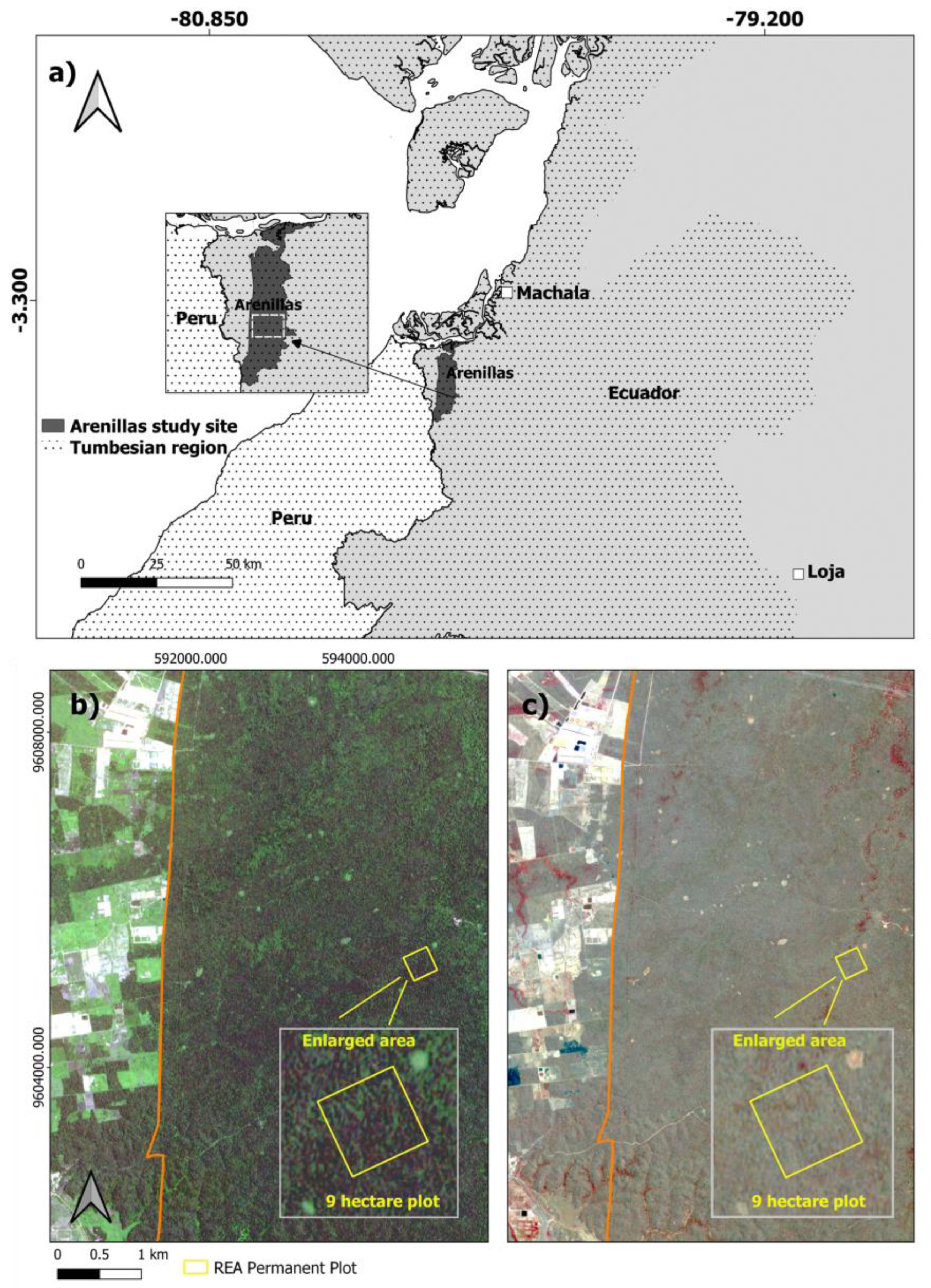
2.1. Study Area

Our 9 ha study site was centered on the 132 km² Reserva Ecologica Arenillas (REA) that is in southwestern Ecuador (Figure 1a). Recognized as a critical piece of the Tumbes-Chocó-Magdalena biodiversity hotspot with high species endemism, REA was included in Ecuador’s national protected areas system in 2001 but was managed as a military base for 60 years prior to 2012 [36]. The study area receives 679 mm of annual rainfall on average. High and low rainfall periods are generally between January and May (139 mm per month) and June and December (15.5 mm per month), respectively, according to 25-year averages (1985–2009) from the Arenillas weather station [37]. Average air temperature ranges between 27 °C during the rainy period and 24 °C during the dry period. SDTF within REA is considered part of the dry scrub and deciduous dry formations that generally cover areas between 0 m to 50 m and 50 m to 200 m in elevation, respectively, within the Tumbesian biogeographic region [38]. Dry forest in these formations commonly includes tree species such as Ceiba trichistandra (Bombacaceae), Tabebuia chrysantha and T. bilbergii (Bignoniaceae), together with Colicodendron scabridum (Capparaceae) and Croton spp. (Euphorbiaceae) [39]. Topography is relatively level within REA; however, many small seasonally wet drainages are present with minor slopes (<10%). Some disturbances such as fuel woodcutting occur within the reserve, as well as seasonal flooding events. The surrounding landscape adjacent to REA is primarily used for agriculture with interspersed patches of remnant forest (Figure 1b,c).

2.2. Tree Data

Tree species, stem diameter, and height were collected within a 9 ha study area that is subdivided into 225 marked, 20 × 20 m (400 m²) plots for systematic tree measurement and orientation. The site was established between 2010 and 2011 and re-measured in 2014. The study area location known as “Pintag Nuevo” on REA is considered a later successional forest with low disturbance in the transition zone between scrub and deciduous formations [36]. All trees were marked with metal tags for relocation and measurement. During the 2011 dry season, all marked trees ≥ 2.5 cm diameter at breast height (DBH = 1.37 m above the tree base) were stem-mapped with Universal Transverse Mercator (UTM, WGS84, Zone 17) coordinates using a Leica total station, model TS02-5 power with a spatial precision of <5 cm. Each tree height was measured separately to the nearest cm using a TruPulse 360° compact laser hypsometer from the base to the highest point of the tree. DBH was measured with a diameter tape to the nearest mm. For our study, we used data from stems measuring ≥5.0 cm DBH to focus primarily on trees and some taller stature shrubs (~2 m to 4 m in height). For simplicity, we refer to all species observed as “trees”. We performed a field survey during April of 2019 to assess the disturbance and sample leaf area index (LAI) at 75 marked subplot corners in the central portion of the 9 ha area using a Decagon ACCUPAR LP-80 (https://www.metergroup.com/, accessed on 16 January 2023). Field LAI measurements were used to make general comparisons with average satellite-image-based LAI measurements for the study area.

2.3. Remotely Sensed Data

We used multispectral data from RapidEye and Sentinel-2 satellite sensors with repeated global coverage. Because RapidEye and Sentinel-2 are aboard multiple satellites, they allow frequent revisit intervals of between 1 to 5 days, respectively, that is important for obtaining cloud-free images. RapidEye is a commercial sensor with high spatial resolution (5 m) and extensive image archives collected since 2008 [31,32]. RapidEye’s spectral bands cover the blue, green, red, red-edge and near infrared (NIR) spectral wavelengths (Table 1). We obtained two relatively cloud-free RapidEye images for April (leaf-on) and September (leaf-off) of 2019 that were preprocessed for making geometric and radiometric corrections.

Previous studies have found that vegetation indices (VI) using a combination of bands to enhance sensitivity to changes in LAI, chlorophyll content and carotenoids are important to SDTF diversity assessment [31,32]. We used a set of indices from prior work, and others such as the modified triangular vegetation index (MTVI2) that is sensitive to chlorophyll content and LAI [40]. We used VIs for leaf-on and leaf-off images interchanging red with red-edge bands to further enhance differences in tree canopy reflectance (Table 1).

Table 1. Spectral bands and VI from RapidEye leaf-on and leaf-off satellite imagery used as predictor variables in ensemble models of α-diversity measures.

Var. Abbrev.	Spectral Range (nm)	Description	Equation	Ref.
b1	440–510	Blue	-	-
b2	520–590	Green	-	-
b3	630–685	Red	-	-
b4	690–730	Red-edge	-	-
b5	760–850	NIR	-	-
ndvi	-	Normalized difference vegetation index	$\frac{NIR - Red}{NIR + Red}$	[41]
ndvir	-	Red-edge normalized difference vegetation index	$\frac{NIR - Rededge}{NIR + Rededge}$	[42]
gndvi	-	Green normalized difference vegetation index	$\frac{NIR - Green}{NIR + Green}$	[43]
rg	-	Red–green simple ratio	$\frac{Red}{Green}$	[44]
sr	-	Simple ratio	$\frac{NIR}{Red}$	[45]
sre	-	Red-edge simple ratio	$\frac{NIR}{Rededge}$	[43]
mtvi2	-	Modified triangular vegetation index	$\frac{1.5\left[1.2\left(NIR - Green\right) - 2.5\left(Red - Green\right)\right]}{\sqrt{\left[{\left(2NIR + 1\right)}^2 - \left(6NIR - 5\sqrt{Red}\right)\right) - 0.5]}}$	[40]
rtvi	-	Red-edge triangular vegetation index	$100\left(NIR - Rededge\right) - 10\left(NIR - Red\right)$	[46]

Table 1. Spectral bands and VI from RapidEye leaf-on and leaf-off satellite imagery used as predictor variables in ensemble models of α-diversity measures.

Var. Abbrev.	Spectral Range (nm)	Description	Equation	Ref.
b1	440–510	Blue	-	-
b2	520–590	Green	-	-
b3	630–685	Red	-	-
b4	690–730	Red-edge	-	-
b5	760–850	NIR	-	-
ndvi	-	Normalized difference vegetation index	$\frac{NIR - Red}{NIR + Red}$	[41]
ndvir	-	Red-edge normalized difference vegetation index	$\frac{NIR - Rededge}{NIR + Rededge}$	[42]
gndvi	-	Green normalized difference vegetation index	$\frac{NIR - Green}{NIR + Green}$	[43]
rg	-	Red–green simple ratio	$\frac{Red}{Green}$	[44]
sr	-	Simple ratio	$\frac{NIR}{Red}$	[45]
sre	-	Red-edge simple ratio	$\frac{NIR}{Rededge}$	[43]
mtvi2	-	Modified triangular vegetation index	$\frac{1.5\left[1.2\left(NIR - Green\right) - 2.5\left(Red - Green\right)\right]}{\sqrt{\left[{\left(2NIR + 1\right)}^2 - \left(6NIR - 5\sqrt{Red}\right)\right) - 0.5]}}$	[40]
rtvi	-	Red-edge triangular vegetation index	$100\left(NIR - Rededge\right) - 10\left(NIR - Red\right)$	[46]

Sentinel-2 imagery has also shown promise for assessing levels of tree diversity in temperate and Mediterranean forest systems [47,48]. Sentinel-2 is a public data source that has a 10 m to 60 m spatial resolution. Broadband visible, red-edge and NIR bands are collected at a 10 m pixel size while separate narrowband red-edge, NIR, and two shortwave infrared bands are collected at a 20 m pixel size (

Table 2. Spectral bands and VI according to Sentinel-2 satellite imagery from leaf-on and leaf-off periods used as predictor variables in ensemble models of α-diversity measures.

Var. Abbrev.	Spectral Range (nm)	Description	Equation	Ref.
b2	458–523	Blue	-	-
b3	543–578	Green	-	-
b4	650–680	Red	-	-
b5	698–713	Red-edge 1	-	-
b6	733–748	Red-edge 2	-	-
b7	773–793	Red-edge 3	-	-
b8	785–900	Near infrared	-	-
b8a	855–875	Near infrared narrow	-	-
b11	1565–1655	Shortwave infrared 1	-	-
b12	2100–2280	Shortwave infrared 2	-	-
evi	-	Enhanced vegetation index	$2.5 \times \frac{\left(NIR - Red\right)}{NIR + 6 \times Red - 7.5 \times Blue+1}$	[50]
ndvi	-	Normalized difference vegetation index	$\frac{NIR - Red}{NIR + Red}$	[41]
rndvi	-	Red-edge normalized difference vegetation index	$\frac{NIR - Rededge 1}{NIR + Rededge 1}$	[42]
rg	-	Red–green ratio	$\frac{Red}{Green}$	[44]
wdvi	-	Weighted difference vegetation index	$IR factor \times NIR - g \times Red factor \times Red$	[51]
lai	-	Leaf area index	$3.618 \times evi - 0.118$	[52]
laib	-	Leaf area index	SNAP biophysical processor 2	[49]
fpar	-	Fraction absorbed photosynthetically active radiation	SNAP biophysical processor 2
fcov	-	Fraction of vegetation cover	SNAP biophysical processor 2
cab	-	Chlorophyll content of leaf	SNAP biophysical processor 2
cw	-	Canopy water content	SNAP biophysical processor 2

² Sentinel Analysis Platform (SNAP).

). We obtained Sentinel-2 imagery for April (leaf-on) and October (leaf-off) of 2019, using the S2MSI1C product from the S2B sensor. For making radiometric corrections, we used the Sentinel Analysis Platform (SNAP) v. 8.0.9 and sen2cor plugin v. 2.05.05. All 20 m bands were resampled to a 10 m pixel size that matched higher resolution bands using nearest neighbor interpolation. The SNAP Biophysical Processor S2 was used to compute LAI, leaf chlorophyll content (CAB), canopy water content (CW), fraction of absorbed photosynthetically active radiation (FAPAR), and fraction of vegetation cover (FCOV) that help distinguish tree species diversity differences associated with site conditions [42,49].

We developed Sentinel-2 VI (Table 2) interchanging red-edge for red bands in addition to developing indices with a wider dynamic range important under dense forest canopy conditions [46]. We calculated mean and standard deviation values for all Sentinel-2 and RapidEye spectral bands and VI at the 0.10 ha plots scale, which have been shown to be important to estimating diversity indices in tropical forest environments [22,53]. Further details about Sentinel-2 and RapidEye spectral bands are provided in the Supplementary 1.

LiDAR height measurements from airborne and satellite platforms have shown to be capable of estimating measures of tropical tree diversity in SDTF and wet tropical environments [16,54]. Due to insufficient LiDAR for the study area, we used tree height and elevation measurements as information often developed with LiDAR from 5129 tree UTM coordinates that were well-distributed across the study area. We used simple kriging to interpolate a ground elevation and canopy height model at a 1 m pixel size. For our elevation surface, we removed extreme low values prior to processing and post processed the raster using a 5 × 5 cell focal mean to reduce anomalous cell values. The same process was applied to tree height values using a 3 × 3 focal mean. From elevation, we derived five topography variables that were aspect, percent slope, topographic roughness, transformed aspect, northness and eastness that are indicators of site biophysical conditions. Three additional canopy height surfaces created were the maximum, minimum and standard deviation of height within a 3 × 3 cell window. We referred to these as interpolated canopy height and topography models, as they were not a direct substitute for vertical profile or ground return information obtained by waveform LiDAR [16]. Interpolation methods for topography and height metrics were developed using the raster and gstat v. 2.0-8 [55] packages for R statistical software v 4.1.2 [56]. For developing combined data sources, we resampled all predictor variables to a 5 m pixel size matching RapidEye.

2.4. Diversity Indices

We used tree species coordinates intersecting each simulated plot to calculate seven α-diversity indices with the R vegan package v. 2.5-7 [57] (

Table 3. Species diversity indices and equations used to calculate indices for each simulated 0.10 ha plot.

Diversity Index	Equation	Description	Abbr.
Shannon’s [58]	$H\prime =-{\displaystyle \sum _{i=1}^S}{p}_{i}lo{g}_b{p}_i$	Uncertainty in predicting a species identity of individuals selected at random, sensitive to variation in rare species	H′
Simpson’s [59]	$D_1=-{\displaystyle \sum _{i=1}^S}{p}_i$	Probability that two species taken at random are the same, sensitive to variation as abundant species. Addition of rare species causes minor variation in D1 values	D1
Inverse Simpson’s [60]	$D_2=\frac{1}{{\mathsf{\Sigma }}_{i=1}^S{p}_i^2}$	Simpson’s transformation so that high values correspond to increased species diversity	D2
Unbiased Simpson’s [61]	$D_3=\frac{1}{n\left(n-1\right)}{\sum }_{i=1}^S{n}_i\left(n_i-1\right)$	Probability of any two individuals of the same species being drawn from an infinite community	D3
Fisher’s alpha [62]	$\alpha = \frac{N\left(1-x\right)}{x}$	Logarithmic series describing the relationship between the number of species and the number of individuals in those species	A
Species richness [58]	$S= \frac{s}{\sqrt{N}}$	Number of species occurrences in a sample	S
Piélou’s Evenness [63]	$J=\frac{H\prime }{\log \left(S\right)}$	The equivalence among species in a community	J

).

The selection of index values to describe the level of diversity is largely dependent on study objectives [23,27]. Although there are similarities among diversity metrics used, each emphasizes different elements of tree diversity on plots. Species richness (S) is the total species number on a site, which does not account for abundance. Shannon’s diversity index (H′) is sensitive to variation in rare species encountered among samples in contrast with Simpson’s diversity index (D1) that is sensitive to variations in abundant species [23]. The inverse of Simpson’s is often used to logically increase its value as diversity increases and has also been called Simpson’s dominance (D2) index [27]. Given their similarity, we used only D2 for our analyses. Unbiased Simpson’s (D3) applies rarefaction to reduce the effect of increasing species richness with increased sample size [61]. Fisher’s alpha (A) diversity index is less affected by common or rare species, is not influenced by sample size (i.e., plot area) and attempts to describe the relationship between the number of species and number of individuals within those species [64]. Evenness describes the equitability of species in a community that is an important measure of diversity quantifying the distribution of abundance for species observed on plots [65]. While showing some dependance on species richness, we used Piélou’s J (J) that is considered a relatively robust unevenness measure [24].

2.5. Sample Design

For sampling tree data and α-diversity indices, we used tree UTM coordinates to simulate 0.10 ha circular plots for training and validating remote sensing-based models. Tree locations were first used to create a large set of circular buffers with a 17.84 m radius and subsequently selecting those fully contained within the 9 ha sampling area. Centroid locations for buffers fully inside the plot were used to select locations at random using distance criteria to decrease overlap. Non-overlapping training sample plots (n = 55) for α-diversity indices were then selected at random using a 30 m minimum distance between plot centers. Validation sample plots (n = 60) were also randomly selected using three separate iterations (20 samples per set) at a minimum distance of 30 m (Figure 2b–d). We used separate selection iterations to improve randomization inside the 9 ha study area and reduce direct spatial overlap between training and validation samples.

A separate validation data set placed 25 regularly spaced plot centroids within the study area using a 60 m minimum distance (Figure 3a,b). We used an increased distance for regularly spaced validation plots to reduce some positive spatial correlation in spectral measurements detected at distances ≤50 m, discussed in Supplementary Figure S2. Plot simulations were developed using the raster v. 3.5-15 [66] and spatialEco v. 1.3-6 [67] packages for R. Samples and index values showed near equal density distribution between training and validation data (Figure 4).

For ensemble model training and validation samples, we extracted mean and standard deviation values for all multispectral bands and VI from each sensor and interpolated canopy height and topography models to all plots. To make spatially explicit model predictions, we used a multi-layer focal function to develop mean and standard deviation value rasters from a 3 × 3 pixel area for all predictors. We ultimately produced a consolidated set of 0.10 ha α-diversity samples from tree data and spatial data layers for model development, evaluation, and spatial prediction outlined in the following section.

2.6. Ensemble Models

We focused principal analyses on assessing the ability of remotely sensed data to predict α-diversity indices using ML regression models. We considered that no one ML approach performs well in all circumstances. Single-model approaches can sometimes require extensive parameter searches or are beset by over- or underfitting data that can reduce prediction generalizability [33,34]. To leverage the capability of different ML approaches we used a stacked ensemble where several moderately tuned component models are combined to develop a single meta-model (Figure 5).

Specifically, we used a selection of ML models known as “base learners”, by applying the “caretList” function in the caretEsemble v. 2.0.1 package for R [68]. The caretList function helps train base learners using identical training data and re-sampling methods. In our case, we used 10-fold cross-validation to re-sample data for model training and testing using a heterogeneous set of base learners. Subsequently, we used the trained model list to create an ensemble using the “caretStack” function. At this step, we applied the lasso and elastic-net regularized generalized linear model (“glmnet”) approach by Friedman et al. [69] for developing the final meta-model using weighted prediction probabilities, $\widehat{y}$, obtained from a linear combination of optimized base learners. This procedure was used with single-sensor or multi-sensor satellite data to develop and compare separate ensemble models for each α-diversity index (Figure 5).

Prior to base learner development, we used recursive feature elimination (RFE) to reduce data dimensionality from many possible predictor variables obtained from remotely sensed data. RFE uses iterative backwards selection methods to recursively eliminate weak or collinear variables [70]. To select an optimized subset of predictors, we used random forest tree functions (“rfFuncs”) to rank predictor variables important to each α-diversity index. An optimized, and reduced set of predictors passed to base model development, was selected from the point at which the minimum root mean squared (RMSE) was reached.

In the list of base learners (Figure 5), we included random forest (RF), gradient boosting (GBM), and extreme gradient boosted linear (XGBL) models, as well as support vector machines (SVM) and quantile regression neural networks (QRNN). Gradient “boosting” is applied to iteratively assess and correct successive model error from independently grown regression tree models. “Bagging” used with RF models applies ensemble learning to grow multiple regression trees in parallel with randomly selected training and test samples to assess predictor variables and model performance [71]. Extreme gradient boosting adds methods to reduce overfitting, such as regularization that decreases model complexity by restricting the size of leaf values in tree-based regression models. The SVM cost model applied the radial basis kernel function to establish a decision boundary and fitting function based on input features [72]. QRNN is a hybrid method between quantile regression and neural networks that takes advantage of both techniques to model data with non-homogeneous variances and non-linear patterns [73]. We assumed that each ML method provided a sufficiently different treatment of model inputs that can enhance generalizability from the ensemble approach. All ML model applications were developed using the caret v. 6.0.90 [74] and caretEnsemble packages in R.

2.7. Data Analysis and Model Validation

We developed and assessed three general model categories that were defined as single sensor models using RapidEye and Sentienl-2 data independently, and multi-sensor models that combined all multispectral and interpolated canopy height and topography models. To evaluate each of these, we first used model training performance from 10-fold cross-validation statistics such as the mean absolute error (MAE), RMSE, and R² goodness of fit, generated from non-spatially overlapping sample data. To make appropriate sensor model comparisons, we used equal default tuning parameters from the caret and caretEnsemble R packages for all component and meta-models.

We made further model comparisons from random and regularly spaced validation plots left out of training, using scatter plots of predicted and observed α-diversity values and goodness of fit statistics. Our goal was to create generalizable models for making robust predictions with separate validation data and each diversity index. Predictor variable importance for each ensemble model and diversity index was calculated with permutational methods for complex predictive models using the DALEX v. 2.3.0 package in R [75]. We used optimized ensemble models for making spatial predictions with each sensor type or combination and α-diversity index to visualize outputs. With these steps, we sought to determine which sensor model and approach performed consistently better than others to estimate tree species α-diversity.

Lastly, we examined the sensitivity of different sensor types to differences in tree species diversity indices, composition, and forest structure. For these analyses, forest structure and composition from field measurements were further compared with levels of α-diversity using multivariate techniques. We used similarity matrices, Mantel, and partial Mantel tests to examine relationships between α-diversity measured on training sample plots (n = 55) and reflectance features extracted from satellite image types [76]. We expected that the hypothesized relationship between species and spectral variability would show a significant Mantel correlation, even when controlling forest structure variation. A Euclidian distance matrix was also used in cases where partial Mantel tests were applied to help control for unmeasured spatial relationships between closely spaced 0.10 ha model training plots (Figure 2a). These analytical steps were taken to enhance our investigation of key relationships between α-diversity measurements, sensor types and forest composition and structure measured from tree data on plots.

3. Results

During field surveys in 2019, we encountered only two recent tree falls creating minor canopy gaps within the study area since 2014 that may have contributed to some unexplained error in α-diversity models and predictions. The mean values for field LAI measures (2.77 ± 0.81) were generally comparable with Sentinel-2 image LAI values (2.37 ± 0.10) for the 9 ha study area, although maximum LAI was higher from fine-scale field measures than from 10 m Sentinel-2 pixels (4.32 vs. 2.65) likely due to fine-scale ceptometer measurements made in the field. The distribution of α-diversity measures from 0.10 ha plots showed good correspondence between all three simulated datasets, which we considered important for making valid model comparisons (Figure 4). From simulated training and random validation plots (n = 115), tree density and basal area averaged 1114 trees per ha and 15.6 m² per ha, respectively, with an average tree height of 7.4 m for trees ≥5 cm DBH comprising of 38 species. Species richness averaged 16 tree species per 0.10 ha plot and ranged from 8 to 25 species. Plot elevation ranged between 32 m and 38 m. Further plot summary information for each α-diversity and forest structure measurement is found in Supplementary 3. Correlation among α-diversity measurements was strongly positive except between species richness, unbiased Simpsons and Piélou’s J that showed positive but lower correlation (Supplementary 3).

Prior to developing base learners, RFE typically reduced the number of variables entering models except for a single case where all Sentinel-2 variables were selected with Fisher’s alpha (A) models (

Table 4. Ensemble model training results and error statistics from 10-fold cross-validation, independent from base ML models, for Sentinel-2, RapidEye, and combined models that included tree canopy height, elevation, and topography data. “SD” refers to the cross-validation standard deviation for model error and goodness of fit statistics.

Dep. Var.	Model	No. Vars 1	RMSE	R2	MAE	RMSE SD	R2 SD	MAE SD
H′	Sentinel-2	28/84	0.17	0.54	0.148	0.06	0.344	0.052
	RapidEye	47/52	0.21	0.53	0.167	0.06	0.244	0.053
	Combined	10/156	0.15	0.66	0.127	0.05	0.160	0.043
D2	Sentinel-2	25/84	1.95	0.53	1.660	0.64	0.282	0.578
	RapidEye	30/52	2.22	0.52	1.840	0.63	0.260	0.546
	Combined	28/156	1.94	0.41	1.590	0.39	0.231	0.34
D3	Sentinel-2	63/84	0.31	0.43	0.024	0.02	0.241	0.012
	RapidEye	36/52	0.03	0.47	0.023	0.02	0.331	0.015
	Combined	51/156	0.03	0.46	0.024	0.02	0.292	0.011
A	Sentinel-2	84/84	1.67	0.35	1.40	0.52	0.203	0.455
	RapidEye	50/52	2.14	0.25	1.70	0.41	0.246	0.311
	Combined	103/156	1.50	0.60	1.21	0.49	0.246	0.413
S	Sentinel-2	77/84	2.19	0.31	2.26	0.339	0.308	0.269
	RapidEye	38/52	3.24	0.36	2.66	0.559	0.277	0.519
	Combined	43/156	2.43	0.60	2.11	1.03	0.285	0.945
J	Sentinel-2	83/84	0.04	0.24	0.03	0.018	0.314	0.012
	RapidEye	44/52	0.04	0.22	0.04	0.017	0.207	0.011
	Combined	124/156	0.04	0.38	0.03	0.015	0.304	0.008

¹ Number of predictor variables selected with RFE for each sensor model over the total number of variables tried.

). In nearly all cases, ensemble models outperformed base learners except for Piélou’s J that showed increased cross-validation error (Supplementary 4). An exploration of model training data revealed no spatial correlation among tree species on plots and that areas with higher α-diversity were often sites with greater tree densities (Supplementary 2). There was a significant positive spatial correlation among plots for Sentinel-2 spectral values on plots <100 m apart and little or significantly negative correlation between plots and RapidEye spectral data for plots ≤75 m apart. Positive and negative spectral correlation among training samples was likely related to spatial resolution differences between Sentinel-2 (10 m to 20 m pixels) and RapidEye (5 m pixels), respectively.

Ensemble model performance from 10-fold cross-validation showed that, in most cases, combined sensor models had higher R² values and similar or lower RMSE for α-diversity indices as compared to single-sensor models (Table 4). In some instances, such as with Inverse Simpson’s (D2), separate Sentinel-2 and RapidEye models showed slightly greater R² values, but equal or increased RMSE and MAE. Random validation data compared well with observed values for combined sensor models that showed better goodness of fit than single sensor ensembles in all cases, including D2 and D3 models (

Table 5. Random (grey shaded) and regularly (unshaded) spaced validation 0.10 ha plot predictions from machine learning ensemble models and validation statistics.

Dep. Var.	Model	R2	Adj. R2	Sigma	F-Stat.	p Value	R2	Adj. R2	Sigma	F-Stat.	p-Value
H′	Sentinel-2	0.52	0.51	0.153	63.3	<0.001	0.24	0.21	0.216	7.4	0.012
	RapidEye	0.45	0.44	0.199	47.9	<0.001	0.2	0.16	0.222	5.66	0.026
	Combined	0.67	0.67	0.155	120.0	<0.001	0.54	0.52	0.168	26.92	<0.001
D2	Sentinel-2	0.41	0.4	1.81	40.0	<0.001	0.18	0.14	2.55	4.9	0.036
	RapidEye	0.44	0.43	2.18	44.8	<0.001	0.35	0.32	2.27	12.4	0.002
	Combined	0.62	0.61	1.81	92.5	<0.001	0.38	0.35	2.22	14.1	0.001
D3	Sentinel-2	0.36	0.35	0.028	32.3	<0.001	0.13	0.09	0.024	3.3	0.083
	RapidEye	0.36	0.35	0.034	32.8	<0.001	0.18	0.14	0.025	5	0.035
	Combined	0.5	0.49	0.03	57.7	<0.001	0.42	0.4	0.02	17	<0.001
A	Sentinel-2	0.20	0.19	1.63	14.8	<0.001	0.20	0.17	1.95	5.9	0.023
	RapidEye	0.26	0.25	1.65	21	<0.001	0.29	0.26	1.26	9.3	0.005
	Combined	0.35	0.34	1.62	31.4	<0.001	0.21	0.17	1.95	5.9	0.023
S	Sentinel-2	0.54	0.54	2.15	69.2	<0.001	0.45	0.42	2.69	18.5	<0.001
	RapidEye	0.42	0.41	2.58	41.5	<0.001	0.48	0.46	2.59	21.6	<0.001
	Combined	0.56	0.55	2.26	72.5	<0.001	0.54	0.52	2.43	27.3	<0.001
J	Sentinel-2	0.22	0.2	0.04	15.9	<0.001	0.31	0.28	0.02	10.27	0.003
	RapidEye	0.28	0.27	0.05	22.8	<0.001	0.09	0.05	0.03	2.24	0.147
	Combined	0.37	0.36	0.04	34.0	<0.001	0.20	0.17	0.03	5.9	0.020

). Regularly spaced validation samples with a greater distance apart showed a lower model fit overall, primarily for Sentinel-2 and RapidEye models (Table 5). Goodness of fit with regularly spaced validation samples also decreased for combined sensor models but showed consistently better goodness of fit than single-sensor models for H, D2, D3, and S. Fisher’s alpha (A) and Piélou’s J showed slightly better goodness of fit with regularly spaced plots only for RapidEye and Sentinel-2, respectively. Some spatial correlation among randomly placed validation plots in the 9 ha study area likely contributed to greater overall model performance (i.e., adj. R²) observed from these comparisons.

In general, α-diversity measurements that were more strongly correlated with species richness exhibited better model performance, such as Shannon’s H′ (r = 0.85) that is sensitive to rare tree species on a site. Scatterplots from combined sensor model predictions compared with random validation data showed a relatively strong positive relationship with other α-diversity measurements except for Piélou’s J (Figure 6a–f). Scatterplots from combined sensor models and regularly spaced validation plots showed similar results, but with fewer test samples to draw from (Figure 7a–f). Piélou’s J showed the lowest model performance at each level of validation except with the Sentinel-2 model and regularly spaced validation samples.

Spatial predictions from the different sensor models showed higher α-diversity values in the upper (northern) half of the 9 ha study area (Figure 8a–c). Combined, Sentinel-2 and RapidEye models were in general agreement in terms of locations showing high and low α-diversity. RapidEye imagery with higher spatial resolution (5 m pixels) showed more discrete differences between areas of high and low diversity. The larger pixel size from Sentinel-2 imagery (10–20 m) rendered a more generalized map of high and low tree diversity that was relatively consistent with diversity measures mapped using RapidEye. Combined sensor model predictions varied in appearance, which was likely dependent on variables selected from individual sensors that contributed most to each prediction. Variable importance measures from combined models indicated that, overall, elevation values were most important to α-diversity predictions (Figure 9a–f). Somewhat unexpectedly, canopy height was not among the top 10 predictor variables for most diversity measures, likely in part because average tree height was positively correlated with elevation (r = 0.54) in the study area. In contrast, mean, maximum and minimum canopy height predictors were among the top 10 variables selected with RFE for species richness, in addition to elevation mean and standard deviation (data not shown). Variable importance measures further indicated that a mixture of bands and VI from the two sensors and seasonal dates were helpful for making accurate predictions (Figure 9a–f). This was clear from combined models where the Sentinel-2 chlorophyl absorption band 2 in the blue light spectrum from the leaf-on period was among the most important variables for Shannon’s H′, Inverse Simpson’s, Unbiased Simpson’s, and species richness predictions. Mean and standard deviation values from red, red-edge and NIR bands from both sensors were alternately important for diversity measures with an exception of Fisher’s Alpha showing elevation as strongly important (Figure 9d). We did not interpret predictors for evenness because of relatively low model performance.

We found that observed α-diversity measurements from simulated plots were, in many cases, under-represented by predicted values at the tails of the value distributions (Figure 10a–f). For example, predicted species richness and related indices did not contain minimum and maximum values observed from plots. Only an unbiased Simpson’s index showed consistently good model performance and predictions spanning the full range of observed values from the combined model. Limitations are likely related to characterizing diversity from all tree species ≥5 cm DBH, some of which reside in the understory of larger trees. We found that validation plots with an increasingly dense understory generally showed higher species richness (Figure 11a,b) that was positively correlated with most diversity indices. Average tree height showed a strong negative correlation with tree density (r = −0.74) that was positively correlated with all α-diversity measures apart from Piélou’s evenness (Supplementary 3).

We relied on matrix comparisons using training data sample data (Figure 2a) to better understand the contribution of spectral reflectance measures from each satellite sensor for assessing α-diversity. We established that α-diversity was not significantly related to the geographic distance between plots but was strongly related to tree species composition that showed a significantly positive relationship with forest structure (i.e., tree height and density) on plots (

Table 6. Mantel and partial mantel test comparing Sentinel-2 and RapidEye spectral data and indices from 0.10 ha randomly spaced training data samples (n = 55) with forest composition, structure, and α-diversity values. The Bray–Curtis distance was used in all cases with the exception of geographic distance measured from plot coordinates that used Euclidean distance.

Matrix Comparisons	Control Matrix	Test	Mantel r	p-Value 1
α-Diversity/Geographic dist.		Mantel	0.05	0.13
α-Diversity/Species comp.		Mantel	0.39	<0.001 ***
α-Diversity/Species comp.	Geographic	Partial mantel	0.39	<0.001 ***
α-Diversity/Forest structure		Mantel	0.23	<0.001 ***
α-Diversity/Forest structure	Geographic	Partial mantel	0.23	<0.001 ***
Species comp./Geographic dist.		Mantel	0.08	0.038 *
Species comp./Geographic dist.	Forest structure	Partial mantel	0.05	0.14
Species comp./Forest structure		Mantel	0.35	<0.001 ***
α-Diversity/Sentinel-2		Mantel	0.13	0.035 *
α-Diversity/Sentinel-2	Geographic	Partial Mantel	0.13	0.045 *
α-Diversity/Sentinel-2	Forest structure	Partial Mantel	0.14	0.034 *
α-Diversity/RapidEye		Mantel	0.08	0.1002
Species comp./Sentinel- 2		Mantel	0.057	0.18
Species comp./RapidEye		Mantel	0.095	0.036 *
Species comp./RapidEye	Forest structure	Partial Mantel	0.054	0.14
Forest structure/Sentinel-2		Mantel	0.05	0.17
Forest structure/RapidEye		Mantel	0.13	0.01 **
Forest structure/RapidEye	Geographic	Partial Mantel	0.12	0.01 **

¹p-Value at significance levels ≤0.05 *, ≤0.01 **, and ≤0.001 ***.

). These complexities were important for interpreting relationships between α-diversity and spectral data. Mantel and partial Mantel tests revealed that in all cases Sentinel-2 spectral data showed a significant relationship with α-diversity measures (Table 6). Sentinel-2 spectral distance remained significantly related to α-diversity when controlling for geographic and forest structure distance among training plots. RapidEye spectral data were not significantly related to α-diversity once it controlled forest structure variables. In contrast, RapidEye showed a significantly positive relationship with the forest structure, while Sentinel-2 did not. Spectral data and VI from either of the two multispectral sensors showed no significant relationship with species composition, when forest structure was controlled using partial Mantel tests (Table 6).

4. Discussion

We found that mixed sensor types provided complementary information for estimating levels of α-diversity in SDTF. With a few exceptions, models using combined sensor data produced consistently lower model error and better goodness of fit for α-diversity measures when compared with single sensor models. Model ensembles typically outperformed those which developed from a single ML approach showing lower cross-validation error and improved fit (Supplementary 4). Satellite imagery with mixed spectral and spatial resolutions contributed distinct information to tree diversity predictions. Sentinel-2 data with a greater number of spectral bands showed a significant relationship with α-diversity measures from Mantel tests that aligned more closely with the spectral variability hypothesis [2,28]. RapidEye bands and indices, in general, showed no direct statistical relationship to α-diversity measures but were significantly related to forest structure (i.e., Bray–Curtis distance) that was indirectly linked to tree diversity indices. Fricker et al. [22] indicate that spectral reflectance patterns from high spatial resolution imagery capture shadow and light gaps that are correlated with vertical forest structure and tree diversity. We found that RapidEye bands and indices are likely impacted by canopy surface roughness and light volume scattering that related significantly to tree height and density. Neither Sentinel-2 nor RapidEye data showed a direct significant relationship with tree species composition on model training plots which, as expected, was statistically related to α-diversity measures (Table 6).

Our results suggest that, in most cases, multispectral satellite imagery was indirectly associated with diversity measures but could adequately capture vegetation and biophysical variation in ways linked to tree diversity [77]. Forest structure differences were strongly correlated with fine-scale topography in our study area. Importantly, the 9 ha study area on REA is in a transitional environment between deciduous dry scrub and tree dominated vegetation [38]. These conditions are conducive to multiple canopy strata and mixed composition SDTF that showed no spatial correlation among tree species on plots near one another (Supplementary 2). Lower elevation sites showing higher α-diversity were an assortment of short-stature and overstory trees with higher tree density relative to upland sites. Correlation comparisons confirmed that elevation was negatively correlated with all α-diversity measures in addition to tree height (Supplementary 3). Mapped predictions showed consistently higher α-diversity levels in lower topography as opposed to uplands sites composed of taller trees with comparatively open sub-canopy structure (Figure 8a–c). We observed that actual α-diversity estimates from validation plots were visually consistent with areas showing high and low α-diversity from spatially explicit predictions (Figure 12a–f). Higher tree diversity values are also generally aligned with lower elevation sites in the study area.

Our findings generally correspond with studies showing that canopy height variables explain a significant proportion of α- and β-diversity for SDTF in areas with differing levels of disturbance [31,54]. Hernández-Stefononi et al. [54] found that SDTF height variability assessed from multi-return LiDAR explained differences in tree species richness. Interpolated canopy height in our study were not among the most important α-diversity predictors, likely because of a moderately positive correlation with elevation. Fine-scale elevation data improved models because of its negative relationship with tree density (r = −0.45) that had a strong positive relationship with tree species richness (r = 0.71). Other topographic variables were less important in our models, which have also shown only minor gains for predicting tree diversity values in temperate forest systems [48]. Nevertheless, the impact of local terrain variability, slope curvature and hillslope position that impact hydrology and solar radiation are potentially important at larger spatial scales [22]. We found that indicators of environmental heterogeneity such as mean and standard deviation in elevation, eastness and northness alternately appeared as important variables for species richness, Shannon’s H′, inverse Simpson’s, and evenness indices (Figure 9a–f), consistent with SDTF field studies on this site [78].

To better understand the relationship between elevation, forest height structure, and α-diversity, we experimentally removed elevation from tree species richness models. We found that minimum and mean tree heights became highly important with little or no model performance loss (Supplementary 5). These results suggest that forest structure assessed from LiDAR can be a strong indicator of tree diversity in SDTF areas even when disturbance is low [79]. Marselis et al. [16] also found that vertical canopy structure assessed from GEDI waveform LiDAR was a reasonable proxy for tree species richness in wet tropical forest. Prior studies using simulated GEDI metrics describing vertical forest structure have shown a similarly significant relationship with Shannon’s H′ and tree species richness [80]. In our study area, forest height structure was likely important to tree diversity differences, although interpolated canopy height data lacked other potentially important and complementary information on vertical canopy structure.

Combined model outcomes and variable contributions were not easily interpreted because of the ensemble approach used, and differences between important predictors for each α-diversity measure. However, our results were comparable to studies in SDTF and other systems that showed improved tree diversity estimates could be obtained using multi-season imagery and mixed sensor types [31,48,80]. Vegetation indices and spectral bands from leaf-off and leaf-on and sensor types were interchangeably important to α-diversity measurements in our study area. Vegetation indices incorporating the red-edge band were often among the top predictors or were the most important variable in the case of inverse Simpson’s index. Ochoa-Franco et al. [31] also found that the RapidEye red-edge band was the most important and statistically significant model covariate related to β-diversity, explaining greater variation in tree diversity than tree canopy height.

Conversely, Sun et al. [81] observed only minor gains from incorporating leaf-on red-edge band into remote sensing plant diversity index values for mixed broadleaf and conifer forest types in parts of China. In our study area, we observed that locations in low topography retained some photosynthetically active plant material during the peak dry season period (Figure 1). These areas contrasted with upland sites showing very little dry season photosynthetic activity and had lower tree diversity. Low topography and biophysical conditions appeared to mediate differences in seasonal phenology related to tree diversity that were better captured by red-edge spectral indices. In addition, Malpighia emarginata, an evergreen shrub or small tree found only in low topography, comprised 8% of the stems counted in the 9 ha area that intermix with other common evergreen species Cynophalla mollis and Colicodendron scabridum. A post hoc assessment of the RapidEye leaf-off red-edge VI only showed a statistically significant relationship with α-diversity measures (Bray–Curtis distance) and partial Mantel tests controlling for geographic (Mantel r = 0.14, p = 0.018) and forest structure (Mantel r = 0.12, p = 0.035) distance. These outcomes suggest that plant phenology and leaf functional traits (e.g., deciduousness, chlorophyll, or nutrient content) captured by seasonal red-edge indices were helpful for distinguishing α-diversity levels [30].

In many cases, spatial predictions were similar between models, diversity indices and validation plots (Figure 8 and Figure 12). Of the six indices examined, Piélou’s J (evenness) was less correlated with other α-diversity indices and showed low predictive capacity from ensemble models. Tree species evenness (relative abundance) is a component of species richness relative to the minimum and maximum number of species observed [24] that is likely constrained by sensor type, number of spectral bands and band widths. In contrast, Redowan [82] found that evenness categories could be accurately predicted for temperate forest types using an artificial neural network classifier with Landsat TM bands and terrain variables. Further work is likely needed to determine how data assimilation methods can better distinguish levels of trees species abundance and differences between sites for tropical areas when a larger number of species are present.

Although we did not specifically examine sampling differences and impacts on α-diversity models with this study, initial comparisons indicated that tree measurements (e.g., plot size and minimum tree diameter used) can strongly influence diversity index values and prediction outcomes. Fricker et al. [22] showed that sub-setting smaller diameter trees and shrubs (<10 cm DBH) improved species richness model predictions from remotely sensed data. We also found that shrubs or short stature trees were important in our models and distinguishing α-diversity differences on simulated plots. Plot size relative to satellite sensor specifications has also proven important for producing robust model predictions [80]. In our case, sensor types with larger pixel sizes produced some spatial correlation between closely spaced plots and spectral data. This may be less a factor for landscape-scale studies with data from forest plots that are widely apart. Nevertheless, incorporating varied sensor specifications into elements of field sampling design developed to capture plant diversity will likely improve model performance [16,22].

Our findings confirm the usefulness of mixed remote sensing platforms for distinguishing some elements of SDTF tree diversity, and not others. Diversity indices correlated with species richness were better predicted by proxy metrics than indices related to evenness that rely on precise estimates of species distribution and abundance. Assimilated spectral bands, seasonal VI, tree canopy height and topography were highly important predictors. Higher tree diversity was positively correlated with differences in forest height structure that occurred within specific topographic environments in our study area. Efforts to harmonize remotely sensed data sources, forest inventories and other field sampling efforts could likely advance broad-scale estimates of tree species diversity [15,83].

5. Conclusions

We established that georeferenced tree census data can provide unique opportunities for examining tropical tree species diversity with information obtained from global remote sensing platforms. From our study, we found that spatial and spectral resolution differences between RapidEye and Sentinel-2 imagery contributed unique information that was related to SDTF tree diversity. Higher spatial resolution RapidEye bands and indices were significantly correlated with tree density and canopy height that were indirectly related to α-diversity measures. Sentinel-2 provided higher spectral resolution data that was more directly correlated with the tree diversity indices examined. Seasonal imagery and vegetation indices from each sensor, useful for distinguishing phenology differences among species present, were frequently important in α-diversity models. Notwithstanding, we found that high resolution digital elevation data related to tree height and composition differences present within distinct topographic environments was vitally important to tree diversity predictions. Each data source routinely provided complementary information to α-diversity models.

Correspondingly important to our study were machine learning applications for variable selection, assimilation, and model development. With 156 possible predictor variables in combined sensor models, recursive feature elimination coupled with ensemble machine learning was efficient for data reduction, model integration and making spatially explicit α-diversity predictions. Optimized variables from multiple sources often resulted in superior model performance. Predicted species richness and tree diversity indices from Shannon’s H′, inverse Simpson’s, and unbiased Simpson’s unambiguously exhibited a stronger relationship with field validation data in comparison with single sensor models. Mapped α-diversity values largely agreed with areas of high and low diversity observed in the study area. The most robust predictions at each validation stage were from combined models for species richness and Shannon’s H′ index, which showed a strong positive correlation with one another (r = 0.85). Indices less affected by sample size, common or rare species (e.g., Fisher’s alpha) showed mixed results, alternately demonstrating better performance with combined and single sensor models when assessed with separate validation data. Model performance was relatively low in all cases for Piélou’s J, a measure of evenness that was not strongly correlated with tree species richness (r = 0.21). Further work and data assimilation methods are likely needed for assessing these and other alternate diversity measures.

Our findings suggest that forest structure and elevation data from global satellites such as GEDI waveform LiDAR and multispectral imagery collected at near-daily intervals, such as PlanetScope 8-band imagery, could enhance methods developed with this study. Greater alignment between tropical forest inventories and information obtained from global remote sensing platforms can likely yield significant gains for assessing SDTF tree diversity at landscape to regional scales. As national and international conservation programs seek to improve tropical forest information needed for attaining biodiversity goals, data integration methods examined here can help fill essential information gaps.

References

1. Foody, G.M.; Cutler, M.E.K. Mapping the species richness and composition of tropical forest from remotely sensed data with neural networks. Ecol. Model. 2006, 195, 37–42. [Google Scholar] [CrossRef] [Green Version]
2. Rocchini, D.; Balkenhol, N.; Carter, G.A.; Foody, G.M.; Gillespie, T.W.; He, K.S.; Kark, S.; Levin, N.; Lucas, K.; Luoto, M.; et al. Remotely sensed spectral heterogeneity as a proxy of species diversity: Recent advances and open challenges. Ecol. Inform. 2010, 5, 318–329. [Google Scholar] [CrossRef]
3. Bustamonte, M.M.C.; Roitman, I.; Aide, T.M.; Alencar, A.; Anderson, L.O.; Aragão, L.; Asner, G.P.; Barlow, J.; Berenguer, E.A.; Chambers, J.; et al. Toward an integrated monitoring framework to assess the effect of tropical forest degradation and recovery on carbon stocks and biodiversity. Glob. Change Biol. 2016, 22, 92–109. [Google Scholar] [CrossRef] [PubMed] [Green Version]
4. Ganivet, E.; Bloomberg, M. Towards rapid assessment of tree species diversity and structure in fragmented tropical forests: A review of perspectives offered by remotely-sensed and field-based data. For. Ecol. Manag. 2019, 432, 40–53. [Google Scholar] [CrossRef]
5. Banda-R, K.; Delgado-Salinas, A.; Dexter, K.G.; Linares-Palomino, R.; Oliveira-Filho, A.; Prado, D.; Pullan, M.; Quintana, C.; Riina, R.; Weintritt, J.; et al. Plant diversity patterns in neotropical dry forests and their conservation implications. Science 2016, 353, 1385–1387. [Google Scholar]
6. Miles, L.; Newton, A.C.; Defries, R.S.; Ravilious, C.; May, I.; Blyth, S.; Kapos, V.; Gordon, J.D. A global overview of the conservation status of tropical dry forests. J. Biogeogr. 2006, 33, 491–505. [Google Scholar] [CrossRef]
7. García Millán, V.E.; Sánchez-Azofeifa, A.; Málvarez García, G.C.; Rivard, B. Quantifying tropical dry forest succession in the Americas using CHRIS/PROBA. Remote Sens. Environ. 2014, 144, 120–136. [Google Scholar] [CrossRef]
8. González-M, R.; García, H.; Isaacs, P.; Cuadros, H.; López-Camacho, R.; Rodríguez, N.; Pérez, K.; Mijares, F.; Castaño-Naranjo, A.; Jurado, R.; et al. Disentangling the environmental heterogeneity, floristic distinctiveness and current threats of tropical dry forests in Colombia. Environ. Res. Lett. 2018, 13, 045007. [Google Scholar] [CrossRef]
9. Linares-Palomino, R. Phytogeography and floristics of seasonally dry tropical forest in Peru. In Neotropical Savannas and Seasonally Dry Forests; Pennington, T.R., Ratter, J.A., Eds.; CRC Press: Boca Raton, FL, USA, 2006; pp. 257–280. [Google Scholar]
10. Manchego, C.E.; Hildebrandt, P.; Cueva, J.; Espinosa, C.I.; Stimm, B.; Günter, S. Climate change versus deforestation: Implications for tree species distribution in the dry forests of southern Ecuador. PLoS ONE 2017, 12, e0190092. [Google Scholar] [CrossRef] [Green Version]
11. Cueva Ortiz, J.; Espinosa, C.I.; Dahik, C.Q.; Mendoza, Z.A.; Ortiz, E.C.; Gusmán, E.; Weber, M.; Hildebrandt, P. Influence of anthropogenic factors on the diversity and structure of a dry forest in the central part of the Tumbesian Region (Ecuador-Perú). Forests 2019, 10, 31. [Google Scholar] [CrossRef] [Green Version]
12. Cueva-Ortiz, J.; Espinosa, C.I.; Aguirre-Mendoza, Z.; Gusmán-Montalván, E.; Weber, M.; Hildebrandt, P. Natural regeneration in the Tumbesian dry forest: Identification of the drivers affecting abundance and diversity. Sci. Rep. 2020, 10, 9786. [Google Scholar] [CrossRef] [PubMed]
13. Rossi, C.; Kneubühler, M.; Schütz, M.; Schaepman, M.E.; Haller, R.M.; Risch, A.C. Remote sensing of spectral diversity: A new methodological approach to account for spatio-temporal dissimilarities between plan communities. Ecol. Indic. 2021, 130, 108106. [Google Scholar] [CrossRef]
14. Cavender-Bares, J.; Schnelder, F.D.; Santos, M.J.; Armstrong, A.; Carnaval, A.; Dahlin, K.M.; Fatoyinbo, L.; Hurtt, G.C.; Schimel, D.; Townsend, P.A.; et al. Integrating remote sensing with ecology and evolution to advance biodiversity conservation. Nat. Ecol. Evol. 2022, 6, 506–519. [Google Scholar] [CrossRef] [PubMed]
15. Dubayah, R.; Blair, J.B.; Goetz, S.; Fatoyinbo, L.; Hansen, M.; Healey, S.; Hofton, M.; Hurtt, G.; Kellner, J.; Luthcke, S.; et al. The global ecosystem dynamics investigation: High resolution laser ranging of the Earth’s forests and topography. Sci. Remote Sens. 2020, 1, 100002. [Google Scholar] [CrossRef]
16. Marselis, S.; Keil, P.; Case, J.M.; Dubayah, R. The use of GEDI canopy structure for explaining variation in tree species richness in natural forests. Environ. Res. Lett. 2022, 17, 045003. [Google Scholar] [CrossRef]
17. Castagneyrol, B.; Jactel, H. Unraveling plant-animal diversity relationships: A meta-regression analysis. Ecology 2012, 93, 2115–2124. [Google Scholar] [CrossRef] [PubMed]
18. Barton, P.S.; Westgate, M.J.; Lane, P.W.; MacGregor, C.; Lindenmayer, D.B. Robustness of habitat-based surrogates of animal diversity: A multitaxa comparison over time. J. Appl. Ecol. 2014, 51, 1434–1443. [Google Scholar] [CrossRef] [Green Version]
19. Cruz-Salazar, B.; Ruiz-Montoya, L.; Ramírez-Marcial, N.; García-Bautista, M. Relationship between genetic variation and diversity of tree species in tropical forests in the Ocote Biosphere Reserve, Chiapas, Mexico. Trop. Conserv. Sci. 2021, 14, 1940082920978143. [Google Scholar] [CrossRef]
20. Wu, J.; Li, H.; Wan, H.; Wang, Y.; Sun, C.; Zhou, H. Analyzing the relationship between animal diversity and remote sensing vegetation parameters: The case of Xinjiang, China. Sustainability 2021, 13, 9897. [Google Scholar] [CrossRef]
21. Roy, D.P.; Kashongwe, H.B.; Armston, J. The impact of geolocation uncertainty on GEDI tropical forest canopy height estimation and change monitoring. Sci. Remote Sens. 2021, 4, 1000024. [Google Scholar] [CrossRef]
22. Fricker, G.A.; Wolf, J.A.; Saatchi, S.S.; Gillespie, T.W. Predicting spatial variations of tree species richness in tropical forests from high-resolution remote sensing. Ecol. Appl. 2015, 25, 1776–1789. [Google Scholar] [CrossRef]
23. Daly, A.J.; Baetens, J.M.; Baets, B.D. Ecological diversity: Measuring the unmeasurable. Mathematics 2018, 6, 119. [Google Scholar] [CrossRef] [Green Version]
24. Jost, L. The relation between evenness and diversity. Diversity 2010, 2, 207–232. [Google Scholar] [CrossRef] [Green Version]
25. Ontoy, D.S.; Padua, R.N. Measuring species diversity for conservation biology: Incorporating social and ecological importance of species. Biodivers. J. 2014, 5, 387–390. [Google Scholar]
26. Soto-Navarro, C.A.; Harfoot, M.; Hill, S.L.L.; Campbell, J.; Mora, F.; Campos, C.; Pretorius, C.; Pascual, U.; Kapos, V.; Allison, H.; et al. Towards a multidimensional biodiversity index for national application. Nat. Sustain. 2021, 4, 933–942. [Google Scholar] [CrossRef]
27. Morris, E.K.; Caruso, T.; Buscot, F.; Fischer, M.; Hancock, C.; Maier, T.S.; Meiners, T.; Müller, C.; Obermaier, E.; Prati, D.; et al. Choosing and using diversity indices: Insights for ecological applications from the German Biodiversity Exploratories. Ecol. Evol. 2014, 4, 3514–3524. [Google Scholar] [CrossRef] [PubMed] [Green Version]
28. Palmer, M.W.; Earls, P.G.; Hoagland, B.W.; White, P.S.; Wohlgemuth, T. Quantitative tools for predicting species lists. Environmetrics 2002, 13, 121–137. [Google Scholar] [CrossRef]
29. Rocchini, D. Effects of spatial and spectral resolution in estimating ecosystem α-diversity by satellite imagery. Remote Sens. Environ. 2007, 111, 423–434. [Google Scholar] [CrossRef]
30. Wang, R.; Gamon, J.A. Remote sensing of terrestrial plant biodiversity. Remote Sens. Environ. 2019, 231, 111218. [Google Scholar] [CrossRef]
31. Ochoa-Franco, A.P.; Valdez-Lazalde, J.R.; Ángeles-Pérez, G.; Santos-Posadas, H.M.; Hernádez-Stefanoni, J.L.; Valdez-Hernández, J.I.; Pérez-Rodríguez, P. Beta-diversity modeling and mapping with LiDAR and multispectral sensors in a semi-evergreen tropical forest. Forests 2019, 10, 419. [Google Scholar] [CrossRef] [Green Version]
32. George-Chacon, S.P.; Dupuy, J.M.; Peduzzi, A.; Hernandez-Stefanoni, J.L. Combining high resolution satellite imagery and lidar data to model woody plant species diversity of tropical dry forests. Ecol. Indic. 2019, 101, 975–984. [Google Scholar] [CrossRef]
33. Lieske, D.J.; Schmid, M.S.; Mahoney, M. Ensembles of ensembles: Combining predictions from multiple machine learning methods. In Machine Learning for Ecology and Sustainable Natural Resource Management; Humphries, G.R.W., Magness, D.R., Huettmann, F., Eds.; Springer Nature: Cham, Switzerland, 2018; pp. 109–122. [Google Scholar]
34. Civantos-Gómez, I.; García-Algarra, J.; García-Callejas, D.; Galeano, J.; Godoy, O.; Bartomeus, I. Fine scale prediction of ecological community composition using a two-step sequential machine learning ensemble. PLoS Comput. Biol. 2021, 17, e1008906. [Google Scholar] [CrossRef] [PubMed]
35. Unger, M.; Homeier, J.; Lueschner, C. Relationship among leaf area index, below canopy light availability and tree diversity along a transect from tropical lowland to montane forest in NE Ecuador. Trop. Ecol. 2013, 54, 33–45. [Google Scholar]
36. Espinosa, C.I.; Jara-Guerrero, A.; Cisneros, R.; Sotomayor, J.D.; Escribano-Ávila, G. Reserva Ecológica Arenillas ¿un refugio de diversidad biológica o una isla en extinción. Ecosistemas 2016, 25, 5–12. [Google Scholar] [CrossRef]
37. Instituto Espacial Ecuatoriano (IEE). Memoria Técnica Cantón Huaquillas, Proyecto: Generación de Geoinformación Para la Gestió del Territorio a Nivel Nacional Escala 1:25.000; Clima e Hidrología; Instituto Espacial Ecuatoriano (IEE): Guayaquil, Ecuador, 2012; 20p. [Google Scholar]
38. Sierra, R. Propuesta Preliminar de un Sistema de Clasificación de Vegetación para el Ecuador Continental; Proyecto INEFAN/GEF-BIRF y EcoCiencia; Editorial Rimana: Quito, Ecuador, 1999. [Google Scholar]
39. Espinosa, C.I.; De la Cruz, M.; Jara-Guerrero, A.; Gusmán, E.; Escudero, A. The effects of individual tree species on species diversity in a tropical dry forest change throughout ontogeny. Ecography 2015, 39, 329–337. [Google Scholar] [CrossRef] [Green Version]
40. Haboudane, D.; Miller, J.R.; Pattey, E.; Zarco-Tejada, P.J.; Strachan, I.B. Hyperspectral vegetation indices and novel algorithms for predicting green LAI of crop canopies: Modeling and validation in the context of precision agriculture. Remote Sens. Environ. 2004, 90, 337–357. [Google Scholar] [CrossRef]
41. Rouse, J.W.; Hass, R.H.; Schell, J.A.; Deering, D.W.; Harlan, J.C. Monitoring the vernal advancement and retrogradation (Green Effect) of natural vegetation. In NASA/GSFC Type III Final Report; Greenbelt: MD, USA, 1973; 371p. [Google Scholar]
42. Gitelson, A.; Merzlyak, M.N. Spectral reflectance changes associates with autumn senescence of Aesculus hippocastum L. and Acer platanoides L. leaves. Spectral features and relation to chlorophyll estimation. J. Plant Physiol. 1994, 143, 286–292. [Google Scholar] [CrossRef]
43. Gitelson, A.A.; Kaufman, Y.J.; Merzlyak, M.N. Use of a green channel in remote sensing of global vegetation from EOS-MODIS. Remote Sens. Environ. 1996, 58, 289–298. [Google Scholar] [CrossRef]
44. Birth, G.; McVey, G. Measuring the color of growing turn with a reflectance spectrometer. Agron. J. 1969, 60, 640–643. [Google Scholar] [CrossRef]
45. Jordan, C.F. Derivation of leaf-area index from quality of light on the forest floor. Ecology 1969, 50, 663–666. [Google Scholar] [CrossRef]
46. Chen, P.; Tremblay, N.; Wang, J.; Vigneaulta, P. New index for crop canopy fresh biomass estimation. Spectrosc. Spectr. Anal. 2010, 30, 512–517. [Google Scholar]
47. Ma, X.; Mahecha, M.D.; Migliavacca, M.; van der Plas, F.; Benavides, R.; Ratcliffe, S.; Kattge, J.; Richter, R.; Musavi, T.; Baeten, L.; et al. Inferring plant functional diversity from space: The potential of Sentinel-2. Remote Sens. Environ. 2019, 233, 111368. [Google Scholar] [CrossRef]
48. Chrysafis, I.; Korakis, G.; Kyriazopoulos, A.P.; Mallinis, G. Predicting tree species diversity using geodiversity and Sentinel-2 multi-seasonal spectral information. Sustainability 2020, 12, 9250. [Google Scholar] [CrossRef]
49. Xie, Q.; Dash, J.; Huete, A.; Jiang, A.; Yin, G.; Ding, Y.; Peng, D.; Hall, C.C.; Brown, L.; Shi, Y.; et al. Retrieval of crop biophysical parameters from Sentinel-2 remote sensing imagery. Int. J. Appl. Earth Obs. Geoinf. 2019, 80, 187–195. [Google Scholar] [CrossRef]
50. Huete, A.; Didan, K.; Miura, T.; Rodriguez, E.P.; Gao, X.; Ferreira, L.G. Overview of the radiometric and biophysical performance of the MODIS vegetation indices. Remote Sens. Environ. 2002, 83, 195–213. [Google Scholar] [CrossRef]
51. Clevers, J.G.P.W. Application of a weighted infrared-red vegetation index for estimating leaf area index by correcting for soil moisture. Remote Sens. Environ. 1988, 29, 25–27. [Google Scholar] [CrossRef]
52. Boegh, E.; Seogaard, H.; Broge, N.; Hasager, C.B.; Jensen, N.O.; Schelde, N.O.; Thomsen, A. Airborne multispectral data for quantifying leaf area index, nitrogen concentration, and photosynthetic efficiency in agriculture. Remote Sens. Environ. 2002, 81, 179–193. [Google Scholar] [CrossRef]
53. Nagendra, H.; Rocchini, D.; Ghate, R.; Sharma, B.; Pareeth, S. Assessing plant diversity in a dry tropical forest: Comparing the utility of Landsat and Ikonos satellite images. Remote Sens. 2010, 2, 478–496. [Google Scholar] [CrossRef] [Green Version]
54. Hernández-Stefanoni, J.L.; Dupuy, J.M.; Johnson, K.D.; Birdsey, R.; Tun-Dzul, F.; Peduzzi, A.; Caamal-Sosa, J.P.; Sánchez-Santos, G.; López-Merlín, D. Improving species diversity and biomass estimates of tropical dry forests using airborne LiDAR. Remote Sens. 2014, 6, 4741–4763. [Google Scholar] [CrossRef] [Green Version]
55. Pebesma, E.J. Multivariable geostatistics in S: The gstat package. Comput. Geosci. 2004, 30, 683–691. [Google Scholar] [CrossRef]
56. R Core Team. R: A language and environment for statistical computing. R Foundation for Statistical Computing, Vienna, Austria. 2021. Available online: https://www.R-project.org/ (accessed on 10 June 2022).
57. Oksanen, J.; Blanchet, F.G.; Friendly, M.; Kindt, R.; Legendre, P.; McGlinn, D.; Minchin, P.R.; O’Hara, R.B.; Simpson, G.L.; Solymos, P.; et al. Vegan: Community Ecology Package. R package version 2.5-7. 2020. Available online: https://CRAN.R-project.org/package=vegan (accessed on 10 June 2022).
58. Shannon, C.E. A mathematical theory of communication. Bell Syst. Tech. J. 1948, 27, 379–423. [Google Scholar] [CrossRef] [Green Version]
59. Simpson, E.H. Measurement of diversity. Nature 1949, 163, 688. [Google Scholar] [CrossRef]
60. Jost, L. Entropy and diversity. Oikos 2006, 113, 363–375. [Google Scholar] [CrossRef]
61. Hurlbert, S.H. The nonconcept of species diversity: A critique and alternative parameters. Ecology 1971, 52, 577–586. [Google Scholar] [CrossRef]
62. Fisher, R.A.; Corbet, A.S.; Williams, C.B. The relation between the number of species and the number of individuals in a random sample of animal population. J. Anim. Ecol. 1943, 12, 42–58. [Google Scholar] [CrossRef]
63. Piélou, E.C. The measurement of diversity in different types of biological collections. J. Theor. Biol. 1966, 13, 131–144. [Google Scholar] [CrossRef]
64. Magurran, A.E. Measuring Biological Diversity; Blackwell Publishing: Malden, MA, USA, 2004. [Google Scholar]
65. Jost, L. What do we mean by diversity: The path towards quantification. Métode 2018, 9, 55–61. [Google Scholar] [CrossRef] [Green Version]
66. Hijmans, R.J. Raster: Geographic Data Analysis and Modeling. R Package Version 3.5-15. 2022. Available online: https://CRAN.R-project.org/package=raster (accessed on 10 June 2022).
67. Evans, J.S. _spatialEco_. R package version 1.3-6. 2021. Available online: https://github.com/jeffreyevans/spatialEco (accessed on 10 June 2022).
68. Deane-Mayer, Z.A.; Knowles, J.E. caretEnsemble: Ensembles of caret models 2019, R Package 2.0.1. Available online: https://CRAN.R-project.org/package=caretEnsemble (accessed on 10 June 2022).
69. Friedman, J.; Hastie, T.; Tibshirani, R. Regularization Paths for Generalized Linear Models via Coordinate Descent. J. Stat. Softw. 2010, 33, 1–22. [Google Scholar] [CrossRef] [Green Version]
70. Bazi, Y.; Melgani, F. Toward an optimal SVM classification system for hyperspectral remote sensing images. IEEE Trans. Geosci. Remote Sens. 2006, 44, 3374–3385. [Google Scholar] [CrossRef]
71. Breiman, L. Random forests. Mach. Learn. 2001, 45, 5–32. [Google Scholar] [CrossRef] [Green Version]
72. Cortes, C.; Vapnik, V.N. Support vector networks. Mach. Learn. 1995, 20, 273–297. [Google Scholar] [CrossRef]
73. Taylor, J.W. A quantile regression neural network approach to estimating the conditional density of multiperiod returns. J. Forecast. 2000, 19, 299–311. [Google Scholar] [CrossRef]
74. Kuhn, M. caret: Classification and Regression Training 2017, R Package Version 6.0-78. Available online: https://CRAN.R-project.org/package=caret (accessed on 10 June 2022).
75. Biecek, P. DALEX: Explainers for Complex Predictive Models in R. J. Mach. Learn. Res. 2018, 19, 3245–3249. Available online: https://jmlr.org/papers/v19/18-416.html (accessed on 8 September 2022).
76. Mantel, N. The detection of disease clustering and a generalized regression approach. Cancer Res. 1967, 27, 209–220. [Google Scholar]
77. Rocchini, D.; Boyd, D.S.; Féret, J.-B.; Foody, G.M.; He, K.S.; Lausch, A.; Negendra, H.; Wegmann, M.; Pettorelli, N. Satellite remote sensing to monitor species diversity: Potential and pitfalls. Remote Sens. Ecol. Conserv. 2016, 2, 25–36. [Google Scholar] [CrossRef]
78. Jara-Guerrero, A.; De La Cruz, M.; Espinosa, C.I.; Méndez, M.; Escudero, A. Does spatial heterogeniety blur the signatura of dispersal sindormes on spatial patterns of woody species? A test in a tropical dry forest. Oikos 2015, 124, 1360–1366. [Google Scholar] [CrossRef]
79. Jara-Guerrero, A.; González-Sánchez, D.; Escudero, A.; Espinosa, C.I. Chronic disturbance in a tropical dry forest: Disentangling direct and indirect pathways behind the loss of plant richness. Front. For. Glob. Change 2021, 4, 723985. [Google Scholar] [CrossRef]
80. Marselis, A.M.; Tang, H.; Armston, J.; Abernethy, K.; Alonso, A.; Barbier, N.; Bissiengou, P.; Jeffery, K.; Kenfack, D.; Labriére, N.; et al. Exploring the relation between remotely sensed vertical canopy structure and tree species diversity in Gabon. Environ. Res. Lett. 2019, 14, 094013. [Google Scholar] [CrossRef]
81. Sun, H.; Hu, J.; Wang, J.; Zhou, J.; Lv, L.; Nie, J. RSPD: A novel remote sensing index of plant biodiversity combining the spectral variation hypothesis and productivity hypothesis. Remote Sens. 2021, 13, 3007. [Google Scholar] [CrossRef]
82. Redowan, M. Spatial patter of tree diversity and evenness across forest types in Majella National Park, Italy. For. Ecosyst. 2015, 2, 24. [Google Scholar] [CrossRef] [Green Version]
83. Marselis, S.M.; Abernethy, K.; Alfonso, A.; Armston, J.; Baker, T.R.; Bastin, J.-F.; Bogaert, J.; Boyd, D.S.; Boeckx, P.; Chazdon, R.; et al. Evaluating the potential of full-waveform lidar for mapping pan-tropical tree species richness. Global Ecol. Biogeogr. 2020, 29, 1799–1816. [Google Scholar] [CrossRef]
Figure 1. The 9 ha study area location within the (a) Arenillas Ecological Reserve (REA) and Tumbesian biogeographic region in southern Ecuador. RapidEye imagery from 2019 displays the (b) leaf-on period (April) using a blue, green, and red band combination, and (c) leaf-off period (September) using a NIR, red and green band combination. An enlarged study area (gray box) for (b,c) shows seasonal differences in greater detail.
Remotesensing 15 00583 g001
Figure 2. Randomly spaced 0.10 ha circulate plots for remote sensing-based α-diversity model (a) training and separate (b), (c,d) model validation sample data with a minimum distance of 30 m apart at plot center. Three separate iterations were used to select random validation samples while reducing spatial alignment with training sample data.
Remotesensing 15 00583 g002
Figure 3. Stem mapped tree species ≥5 cm DBH from (a) across the sampling area and (b) within simulated 0.10 ha validation plots regularly spaced at 60 m apart for assessing α-diversity model predictions. Tree location UTM coordinates in (a) with height and elevation measurements were also used to develop tree canopy height and elevation models.
Remotesensing 15 00583 g003
Figure 4. Model training and validation data density distributions from simulated random and regularly spaced 0.10 ha validation plots and values for (a) Fisher’s alpha, (b) Piélou’s evenness, (c) inverse Simpson’s, (d) species richness, (e) Shannon’s H′, and (f) unbiased Simpson’s on the x-axis.
Remotesensing 15 00583 g004
Figure 5. Workflow for data and ensemble model development, assessment, and comparison.
Remotesensing 15 00583 g005
Figure 6. Observed versus predicted diversity index values for 0.10 ha random validation plots from the combined ensemble models using Sentienl-2, RapidEye, and canopy height and topography predictor variables.
Remotesensing 15 00583 g006
Figure 7. Observed versus predicted diversity index values for 10th ha regular validation plots from the combined ensemble models using Sentienl-2, RapidEye, and canopy height and topography predictor variables.
Remotesensing 15 00583 g007
Figure 8. Spatially explicit α-diversity predictions mapped using (a) combined satellite sensors and interpolated canopy height and topography variables, (b) Sentinel-2 only, and (c) RapidEye only ensemble models. Elevation contour lines (gray) are spaced at 3 m intervals.
Remotesensing 15 00583 g008
Figure 9. Variable importance plots for combined ensemble models and each α-diversity measure from n = 25 model permutations with test sample data. Predictor variable names beginning with “r.” were developed from RapidEye. A “.o” or “.f” indicated if a predictor is from the leaf-on or leaf-off period respectively. All “ht.” or “el.” are canopy height and elevation predictors. A suffix of “.mn” or “.sd” indicates mean and standard deviation grid cell values, respectively.
Remotesensing 15 00583 g009
Figure 10. Observed α-diversity index values compared with the range of predicted pixel values from the combined spatial model for regularly spaced 0.10 ha validation plots.
Remotesensing 15 00583 g010
Figure 11. Violin plots of (a) tree height and (b) tree diameter distributions comparing regularly spaced 0.10 ha validation plots (n = 25) grouped by lower (<15), medium (15 to 19), and higher (≥20) species richness.
Remotesensing 15 00583 g011
Figure 12. Regularly spaced 0.10 ha validation plots colored by α-diversity values (a) Shannon’s H′, (b) inverse Simpson’s, (c) unbiased Simpson’s, (d) Fisher’s alpha, (e) species richness and (f) Piélou’s J (evenness) overlaying elevation data and 3 m contours. High to low elevation is represented by dark gray to lighter background colors, respectively.
Remotesensing 15 00583 g012