1. Introduction
Over the past few years, aerial and satellite remote sensing technology has advanced significantly, leading to a rapid increase in the number of remote sensing images. This trend has created a greater need for more efficient and accurate methods to analyze remote sensing images. Semantic segmentation is a critical aspect of remote sensing image processing that significantly enhances its efficiency and the utilization of remote sensing data. Unlike regular images, remote sensing images typically have high resolution and include spatial, spectral, and temporal data, which makes them highly detailed. Therefore, extracting contextual relationships when performing semantic segmentation of remote sensing images is crucial.
For a long time, convolutional neural networks (CNNs) have been the mainstream methods for semantic segmentation. The exceptional performance of FCNs (fully convolutional networks) [
1] has led to the development of their high-achieving successors [
2,
3,
4,
5], which have made CNNs the prevailing approach for semantic segmentation of general images. Recent advancements in CNNs, such as ConvNeXt [
6], HorNet [
7], and InternImage [
8], have significantly improved the performance of CNNs, even surpassing that of transformers, in the general field of semantic segmentation.
Recently, transformers [
9] have been used in computer vision tasks. Vision transformers [
10,
11,
12,
13] are a special type of transformer designed for image processing. They are powerful tools for modeling long-range dependencies, based on the self-attention mechanism that was first introduced in natural language processing. The ViT [
10] was the first vision transformer and became a trendsetter with strong potential, but the enormous computational complexity during training and fine-tuning is not acceptable. To address this problem, hierarchical transformers with the encoder–decoder paradigm were designed, and measures like deformable attention (Deformable DETR by Xia et al. [
13]) and windowed attention (Swin Transformer by Liu et al. [
12]) were adopted either separately or together. However, transformers are less effective in extracting detailed features from RSI because of the massive computation resources required and the lack of spatial inductive bias.
In the recent literature, frequency domain analysis has been introduced in the field of semantic segmentation to address the problem of semantic information loss during the process. This approach has produced promising results using different types of transforms, including discrete Fourier transform (DFT) [
14,
15,
16,
17,
18], discrete cosine transform (DCT) [
19,
20,
21], and discrete wavelet transform (DWT) [
22,
23,
24,
25,
26]. These methods can effectively extract low-frequency and high-frequency image components for separate processing. However, they still have issues such as poor generalization and high computational complexity.
In our paper, we introduce a new architecture called Hierarchical Wavelet Feature Enhancement (WFE), which is based on discrete wavelet transform (DWT). The WFE module performs a multi-scale, lossless decomposition of the input image, which allows it to preserve the high-frequency information. By reintroducing the high-frequency sub-bands back into the original architecture, the WFE module enhances the performance of the architecture. The best part is that the WFE module can be easily integrated into existing convolutional neural networks (CNNs) and transformers without requiring any additional pre-training.
Compared to the time and computation cost required for designing a new semantic segmentation network, WFE modules are relatively simpler and can be easily integrated into existing state-of-the-art pyramid-based semantic segmentation networks. Our model can enhance the performance with minimal increase in structural complexity and computational cost due to the lightweight computation of this architecture. We have conducted tests on remote sensing datasets using popular transformer architectures like Swin Transformer and SegFormer, as well as CNN architectures such as ResNet and ConvNeXt, and have achieved promising results.
2. Related Work
In this section, we briefly review recent advances in semantic segmentation methods specialized for remote sensing images, particularly those related to the frequency domain.
2.1. Methods on Semantic Segmentation of Remote Sensing Images
Semantic segmentation in remote sensing images is different from that of ordinary images, as it involves many details due to its high-resolution nature. In the field of CNN–transformer fusion, several authors have attempted to improve the observed performance. Zhang et al. [
27] created an adapter to fuse convolutional layers and attention modules, specifically, the deformable attention from Deformable DETR [
13] and Mask2Former [
28]. Meanwhile, Chen et al. [
29] proposed a similar fusion approach that is dependent on the backbone of UNet. In contrast, multi-scale channel attention is applied to this architecture. However, the efforts to enhance overall performance have been limited, likely due to the inherent defects of CNNs and transformers that still need to be addressed. Other methods of improvement have also been discovered, including the one proposed by Zhang et al. [
30], where an extension of the SE module [
31] was applied to extract channel features out of transformers. Although our methods are similar, their module is too complex as it involves more learnable parameters. Fang et al. [
32] introduced a creative method that successfully trained a CRENet with a detail head, an LFEAM module, and a superpixel affinity loss to capture both local and global features. Although this plugable module achieved good results, it is highly complex and requires a significant amount of training techniques, making it less desirable in terms of portability. However, none of the above-mentioned works exploited the high-resolution nature of remote sensing images and adopted measures to deal with fine-grained details. In contrast, our approach in the frequency domain has the potential to outperform theirs in processing details.
2.2. Methods Based on DFT
Discrete Fourier transform (DFT) is a powerful tool used for signal and image analysis. By transforming spatial information into frequency information, DFT enables the application of various operations. In the field of semantic segmentation, MsaNlfNet [
14] and FSLNet [
15] concatenate the real and imaginary parts of feature maps, followed by point-wise weighting to learn contextual information in the frequency domain. Another approach proposed by Zhang et al. [
16] is the CSA module that applies DFT in the transformer structure. In this method, the real and imaginary parts are processed separately before being fed into the attention module. In unsupervised learning, Yang et al. [
33] proposed the FDA method that uses DFT in unsupervised models, while Tang et al. [
17] applied DFT in knowledge distillation with a method called Target-Category. Recently, Huang et al. [
18] introduced AFFormer, a frequency-adaptive filtering module that achieves the effect of DFT with lower computational complexity compared to CNNs. However, AFFormer has difficulty fitting images of different sizes. In contrast, our method does not require the processing of complex numbers, resulting in lower computational complexity.
2.3. Methods Based on DCT
Discrete Cosine transform (DCT) is a well-established technique used in image and video compression. Currently, DCT is mainly utilized for compressed images and unsupervised learning. EDANet, introduced by Lo et al. [
19], constructs perceptrons on DCT components of compressed JPEG images. Huang et al. proposed FSDR [
20], which applies DCT in unsupervised training. On the other hand, Pan et al. [
21] incorporated DCT into ResNet, but this research is limited to image classification. To date, supervised learning using DCT is not widely employed.
2.4. Methods Based on DWT
Our module relies on a more innovative method called the DWT, which is used for analyzing signals or images. In their study, Liu et al. [
22] replaced pooling operations with DWT modules for downsampling and used inverse DWT for upsampling. This technique ensured lossless downsampling. Li et al. [
23] used skip connections in the WaveSNet model to concatenate the high-frequency components generated by the DWT to the corresponding upsampling positions, thereby preserving high-frequency information. Su et al. [
24] processed the high- and low-frequency components generated by DWT separately, while processing aerial images; Azimi et al. [
25] used multi-level DWT to concatenate the high-frequency features of different resolutions to the feature map. This helped supplement the information lost by downsampling. An impressive way to enhance transformers is Wave-ViT [
26], where Yao et al. improved ViT by using DWT as the downsampling operation, achieving lossless downsampling, and reducing the number of parameters in the self-attention module.
However, these advancements are highly specialized and cannot be applied to new encoders. In contrast, our method is compatible with various encoders such as Swin Transformer [
12], SegFormer [
11], ConvNeXt [
6], and ResNet [
34].
3. Method
This section briefly introduces the 2D-DWT, which forms the basis of our method. This is followed by the Hierarchical Wavelet Feature Enhancement (WFE) module, the core of our approach.
3.1. Discrete Wavelet Transform
Discrete wavelet transform (DWT) is a popular time–frequency representation of a signal. It improves upon Fourier transform by addressing the issue of representing temporal-frequency dependencies. Through DWT, target signals are decomposed into a combination of wavelets, or small waves. In recent times, wavelet theories have significantly advanced and have become the mainstream in the fields of signal processing and file compression. In this paper, DWT refers to discrete Haar wavelet transform, which is the simplest form of wavelet transform. Other deterministic wavelets or adaptive wavelets are yet to be considered.
3.1.1. The 2D-DWT
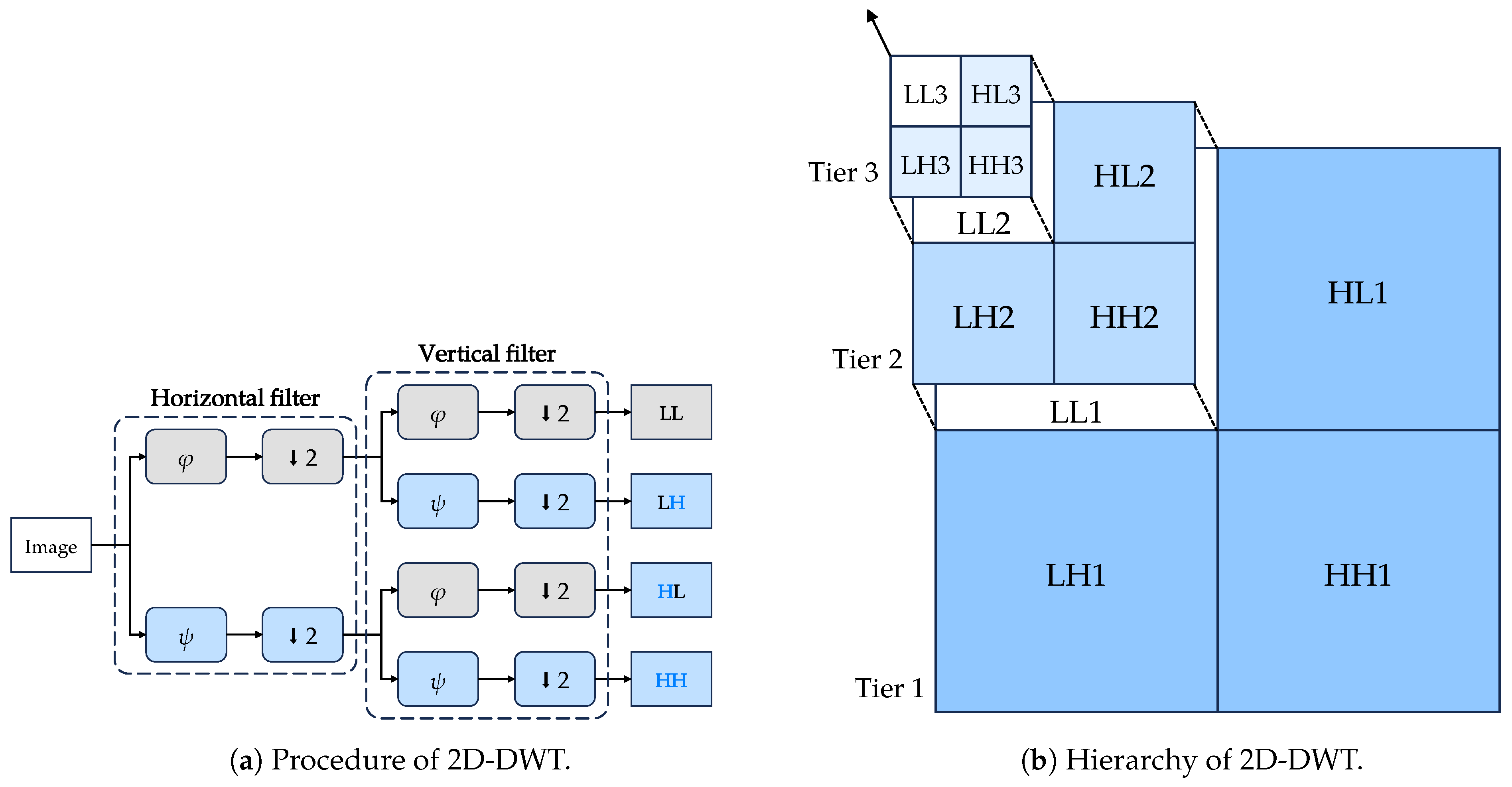
The 2D-DWT approach is an extension of the 1D-DWT, which is a powerful tool for multi-scale analysis of signals and is widely used in image processing. It decomposes an image into four sub-bands, consisting of the low–low (LL), low–high (LH), high–low (HL), and high–high (HH) sub-bands. The 2D discrete wavelet transform (DWT) is lossless and reversible, which means the original image can be fully recovered from the transformed image without any edge problems or loss of information; but we do not apply the inverse 2D-DWT in our proposed model for a specific reason, which will be explained later. As a separable transform, 2D-DWT can be independently applied to the rows and columns of an image. In addition, 2D-DWT is a hierarchical transform, which means that the LL sub-band can be further decomposed into four sub-bands and so on. The 2D-DWT can be interpreted as a series of low-pass and high-pass filtering operations, followed by downsampling by a factor of two.
In the process shown in
Figure 1a, the low-pass filter,
, and the high-pass filter,
, are applied to the rows of the image followed by downsampling by a factor of two. Then, the exact operation is repeated on the columns of the image.
Figure 1b illustrates the hierarchy of the entire transform. In our implementation, we treat filtering as convolutions. Given that 2D-DWT is a linear transform, one different interpretation is that the image passes through four different convolutional layers, each with different kernels. Specifically, the convolution is applied with stride 2 and no padding. For Haar wavelets, the four kernels are, respectively,
This greatly simplifies the process by turning the transform into a few filtering operations, which fits well into the PyTorch [
35] architecture.
3.1.2. Comparison: 2D-DWT vs. 2D-DFT
The 2D-DWT, like 2D-DFT, is a useful tool for extracting high-frequency features from images, including edges and textures. These features are often lost during downsampling operations in convolutional neural networks (CNNs) and transformers. Compared to 2D discrete Fourier transform (DFT), 2D-DWT has several advantages.
The 2D-DWT method preserves the positional information of the features. This means that the transformed image maintains the same size as the original image, allowing for direct manipulation of frequency information at specific positions in the original image. Consequently, our method does not require the inverse, DWT.
The 2D-DWT is a real transform that eliminates the need to process complex numbers, unlike the 2D-DFT which is a complex transform.
The 2D-DWT is a hierarchical transform, which means the transformed image can be further decomposed into four sub-bands and beyond. This is a useful property that will be discussed in the next section.
The 2D-DWT has lower computational complexity than 2D-DFT. The fast implementation of DWT (or FWT) has time complexity of , whereas DFT (or FFT) has time complexity of .
3.2. Hierarchical Wavelet Feature Enhancement (WFE)
3.2.1. Motivation
The 2D-DWT is a hierarchical transform, allowing the transformed image to be further decomposed into four sub-bands, and so on. As a result, the transformed image can be viewed as a hierarchical representation of the original image.
Given that the mainstream CNNs and transformers are hierarchical models, and the 2D-DWT is also a hierarchical transform, we can combine the 2D-DWT with CNNs and transformers to create a hierarchical model. This approach allows us to extract high-frequency features from the image and then feed them to the CNNs or transformers to enhance the features.
Additionally, the semantic information in the images, both high and low frequency, can be lost while downsampling. The DWT operation transforms the semantic information into wavelet–domain maps with reduced spatial size and increased channel count, while, as a lossless operation, preserving all information. As the wavelet representation of images captures both spatial and frequency information, operations on the wavelet domain can produce better results. Inputting them to the feature map with the same resolution proves to be effective and efficient in compensating for the lost semantic information.
Regarding feature enhancement, the DWT has some decided advantages compared with DFT and DCT: (1) the produced wavelet–domain components are still representative in terms of spatial information, making it possible to directly use the DWT-transformed information in the original path, without the need to perform point-wise multiplication, multi-layer perception, or inverse transform; (2) the transform can be performed hierarchically, which lays the foundation of its compatibility with existing hierarchical image networks. The DWT produces consistent output resolution across all levels, enabling easy weighted averaging without interpolation.
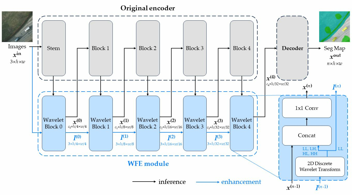
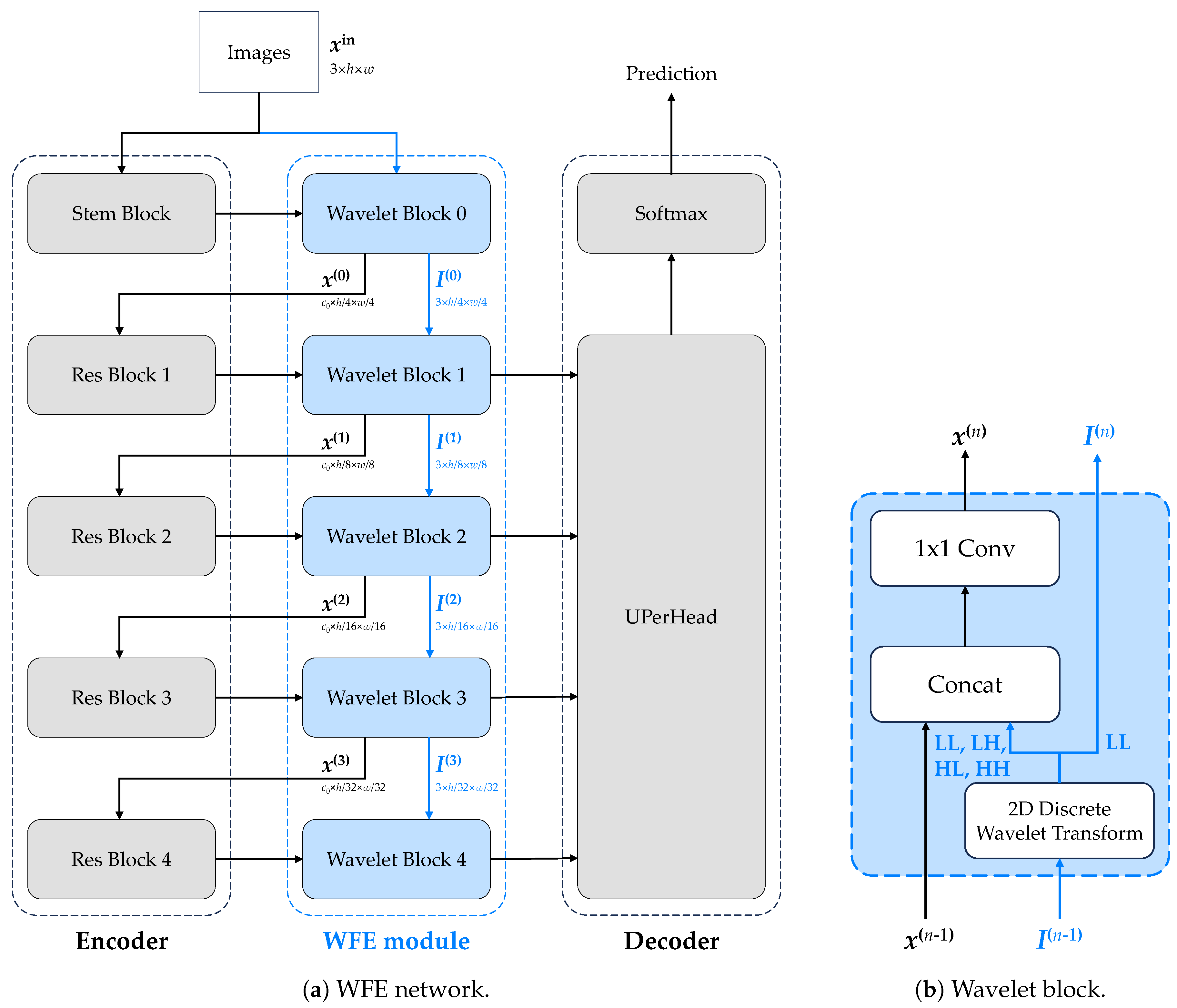
3.2.2. Framework
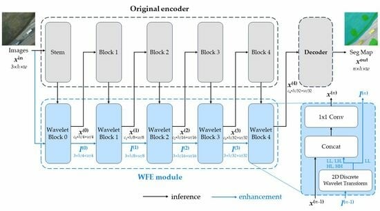
Our method’s framework is illustrated in
Figure 2. First, the input image goes through a 2D-DWT transformation, which is then weighted by learnable parameters, and forwarded to the backbone of the CNNs or transformers. Next, the LL part of the transformed image is sent to the next level of the 2D-DWT, and the same process is repeated. This continues until the transformed image becomes too small to be sent to the CNNs or transformers.
The transformed image is fed to the CNNs or transformers, on the corresponding level of the 2D-DWT, so that the size of the transformed image is the same as the size of the input image of that layer. Then, convolution is applied to the transformed image, to reduce the number of channels to the same as the input image of that layer. Finally, the transformed image is added to the input image of that layer, to enhance the features of the input image.
The classic pyramid hierarchical framework manages to extract high-level features while greatly reducing the time and spatial complexity of the model. However, as mentioned in
Section 3.1, multiple downsampling operations may lead to the loss of certain semantic information in the input image or feature map. For instance, the average pooling operation may cause the loss of high-frequency image information, making the boundary not ideally segmented.
To alleviate this problem, in our WFE module, the input image undergoes multiple DWT operations and is concatenated into the original model feature map when its resolution reached the same size as the original model hierarchy, to replace the semantic information lost in the downsampling operation. Additionally, to improve the universality of WFE modules, the overall structure is independent of the original model architecture and connected with
convolution through channel concatenation, as shown in
Figure 2b.
The 2D-DWT method is only applied to the input image rather than the feature maps of the CNNs or transformers, because the 2D-DWT is a linear transform whereas feature maps of the CNNs or transformers are usually nonlinear. As a result, the 2D-DWT is not suitable for the feature maps of the CNNs or transformers. Besides, if 2D-DWT is applied to the feature maps produced by the backbone, then it is inevitable to consider the large increase in channels, and subsequently, the increase in trainable parameters and model size.
3.2.3. Implementation
Figure 2 illustrates the implementation of our method. The input image is processed through two branches—the blue branch and the black branch. The blue branch represents the discrete wavelet transform (DWT) branch, and the black branch represents the feedback branch. Each wavelet block consists of a 2D-DWT layer. The blue branch on the left encompasses all four sub-bands, while the blue branch on the right includes only the LL sub-band. The transformed image is then forwarded to the next level of the 2D-DWT followed by performing the same operations.
We implemented a custom 2D-DWT layer instead of using the PyTorch Wavelet Toolbox version, because the latter is not differentiable to be used in the training process. The 2D-DWT layer is implemented using the 2D convolutional layer, with the kernels defined in Equation (
1). We added the WFE module to the original backbone architecture and fine-tuned the entire model, with the learning rate adjusted. It is worth noting that the WFE branch is not linked to the decoder, but rather to the original backbone, as shown below:
The position embedding layer in transformers is a linear projection, to which WFE blocks have no connection whatsoever.
The initial downsampling layer (aka the stem layer) usually performs a downsampling operation in different ways. If that operation is performed through two convolutions with strides of 2, then a WFE module is added between those convolutions; otherwise, if it is performed through one pooling, then no WFE module is added.
For other blocks in the encoder, namely Blocks 1 through 4, a WFE block is attached to the output end of each.
Therefore, for each architecture, a total of 4 or 5 WFE blocks are implemented, depending on the type of the stem layer.
The WFE branch feedback is always before skip connections between the encoder and the decoder, making full use of our enhancement module.
4. Experiments
In this section, we conduct experiments on the ISPRS Potsdam and the ISPRS Vaihingen datasets, to evaluate the effectiveness and efficiency of our method. In addition, we compare the performance and the computation cost of our method with other methods that apply frequency domain analysis to semantic segmentation.
4.1. General Experimental Setups
This section introduces the general experimental settings in detail.
4.1.1. Implementation Details
Our method is implemented using the PyTorch framework and the mmsegmentation library. Prior to training, we resize the images to pixels and normalize them using the mean and standard deviation of the ImageNet dataset. During training, we use the Adam optimizer with a specified learning rate, a weight decay of 0.01, and a momentum of 0.9. The batch size is set to 4, and the models are trained on a single NVIDIA GeForce RTX 3090 GPU with 24 GB of memory. For ISPRS Potsdam, the models are trained for iterations, while for ISPRS Vaihingen, they are trained for iterations. We use a polynomial learning rate scheduling scheme with a power of 1 and a 1500 iteration warm-up. It is important to note that all the parameters of the 2D-DWT are fixed during training, and all parameters are consistent with the original papers.
4.1.2. Pre-Training and Diagonal Initialization
The models used for semantic segmentation are pre-trained on the ImageNet dataset, just like they were in the original papers. To initialize the Wavelet blocks in the WFE structure, a diagonal initialization method is used. This means initializing the weights of the Wavelet blocks with the diagonal elements of the corresponding convolutional layers. The reason for this is to ensure that the Wavelet blocks do not modify the features extracted by the convolutional layers during initialization. This helps to ensure the stability of the training process.
4.1.3. Evaluation Metrics
In this part, we elaborate the evaluation metrics. We use OA, mIoU, and mF1 to evaluate our results. In the following equations,
stands for classes, whereas
N stands for all classes except clutter; in our experiments,
. The subscripts
k in Equations (
3), (
5)–(
7) represents the
kth class.
H is the confusion matrix, where elements
represents the amount of pixels whose ground truth is the
ith class while being predicted by the model to be the
jth class.
For both datasets, we use OA as the main metric for evaluation, defined by Equation (
2). OA represents the overall performance of a certain model.
Given that differences of OA on different models may not be apparent, we use mIoU and mF1 as supplementary metrics, as they better reflect the visual appearance of the segmentation. IoU is defined by Equation (
3).
mIoU is the IoU averaged across all classes (includes clutter), defined by Equation (
4).
For mF1, we first define precision in Equation (
5) and recall in Equation (
6).
Then based on those, we define F1 in Equation (
7).
mF1 is defined as the average F1 across all classes (excludes clutter), in Equation (
8).
4.2. Experiments on ISPRS Potsdam
In the following section, we elaborate our experiment conducted on ISPRS Potsdam.
4.2.1. ISPRS Potsdam Dataset
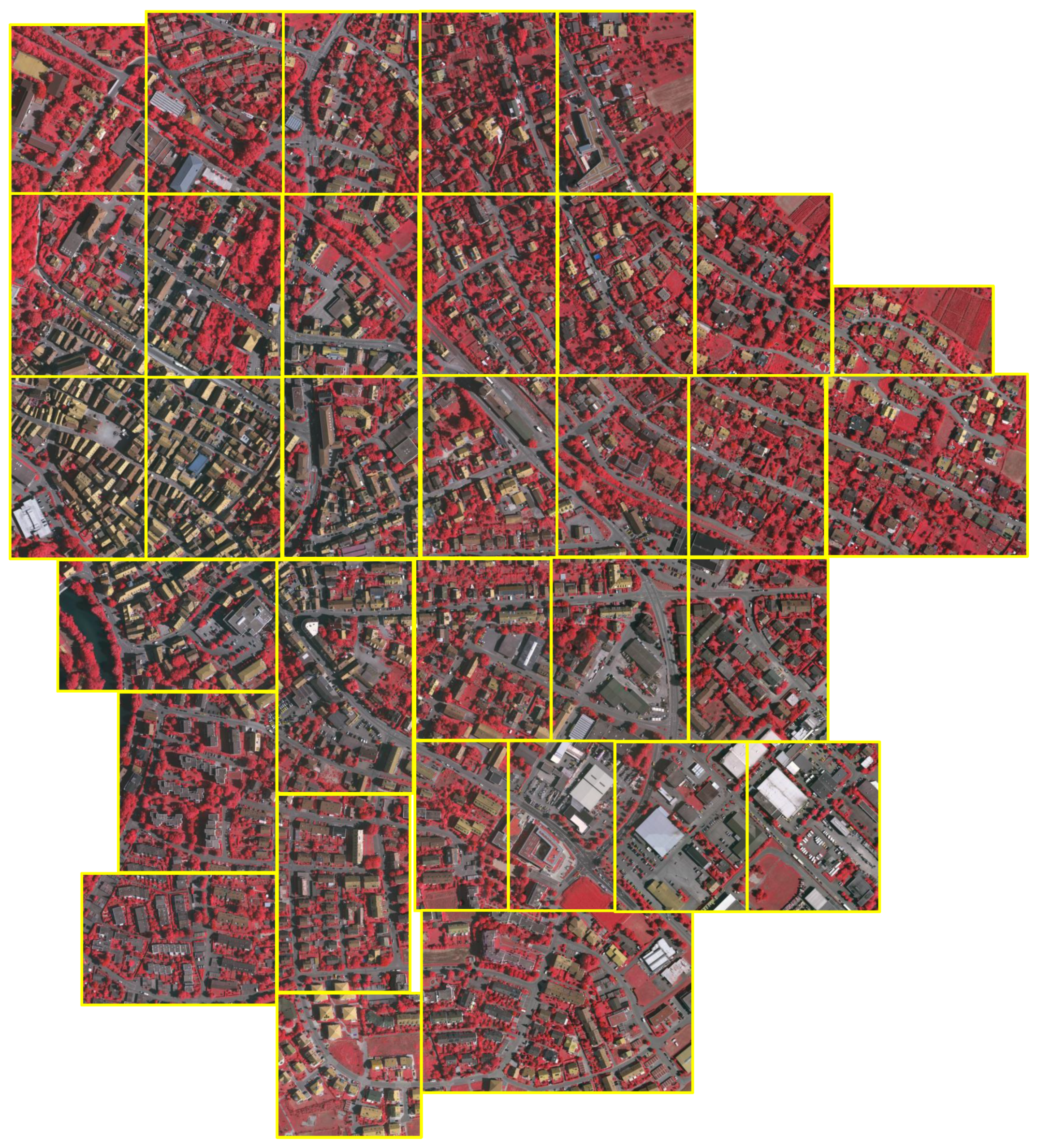
The ISPRS Potsdam dataset, shown in
Figure 3, is a widely-used dataset for semantic segmentation of RSI. It contains 38 ortho-rectified images of the city of Potsdam, Germany, with a spatial resolution of 5 cm, and a size of
pixels. The images are divided into 24 and 14 images for training and validation, respectively. The images are annotated with six classes: impervious surfaces (imp surf), building, low vegetation (low veg), tree, car, and clutter.
During the training, we crop the images to pixels (allow overlapping at the edges), and randomly flip the images horizontally and vertically, thus producing 3456 images for training and 2016 images for validation.
4.2.2. Experimental Settings on ISPRS Potsdam
We conducted experiments on the ISPRS Potsdam dataset to evaluate the effectiveness and efficiency of our method. For transformers, we used Swin Transformer [
12] and SegFormer (MiT) [
11] as the backbone models. For CNNs, we used ResNet [
5], ConvNeXt [
6], and the most recent InternImage [
8] as the backbone models. As to the decode head, we used UPerNet [
5] as the standardized decode head model (except for SegFormer). In addition, we used DeepLabV3+ [
4] as a comparable decode head model, to test whether the decode heads have any impact on our method.
4.2.3. Results on ISPRS Potsdam
The results presented in
Table 1 indicate that the adoption of the WFE module has led to significant improvements in the performance of the original models that are based either on CNNs or transformers. The improvements are more noticeable in the models based on CNNs, which saw an increase of roughly 0.4% in OA, than in those based on transformers, where the increase was roughly 0.1% in OA. This is because the CNNs are more sensitive to high-frequency information, which is preserved by the WFE module. The WFE module requires little additional computation, as it only involves four–five
convolutions, resulting in 0.2% (Swin) to 8% (ResNet) increase in parameters and 1% (Swin)–10% (ResNet) increase in float-point operations. The WFE module has shown that it can be generalized into different models with little additional computation and improve the performance of the original models in the context of remote sensing images. Furthermore, our module surpassed the original architectures based on different backbone sizes, on both CNNs and transformers, and on the earliest and latest purposed models. It also showed a performance boost regardless of the decoder, as demonstrated by the results of UPerNet−ResNet50 and DeepLabV3+−ResNet50.
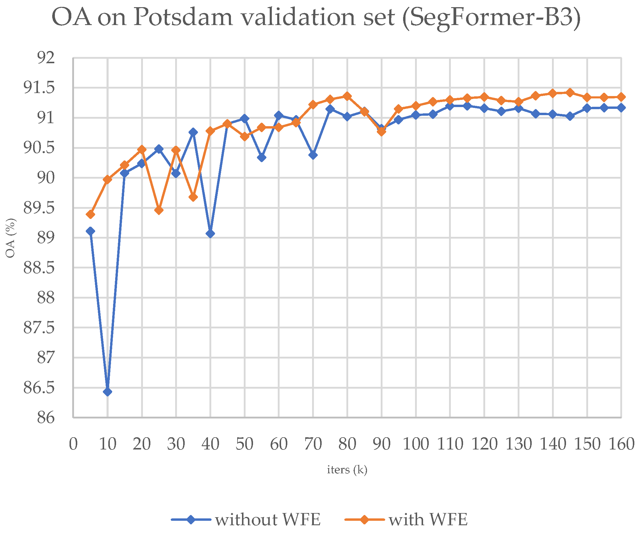
We present the training OA curve in
Figure 4 and the sample results in
Figure 5 and
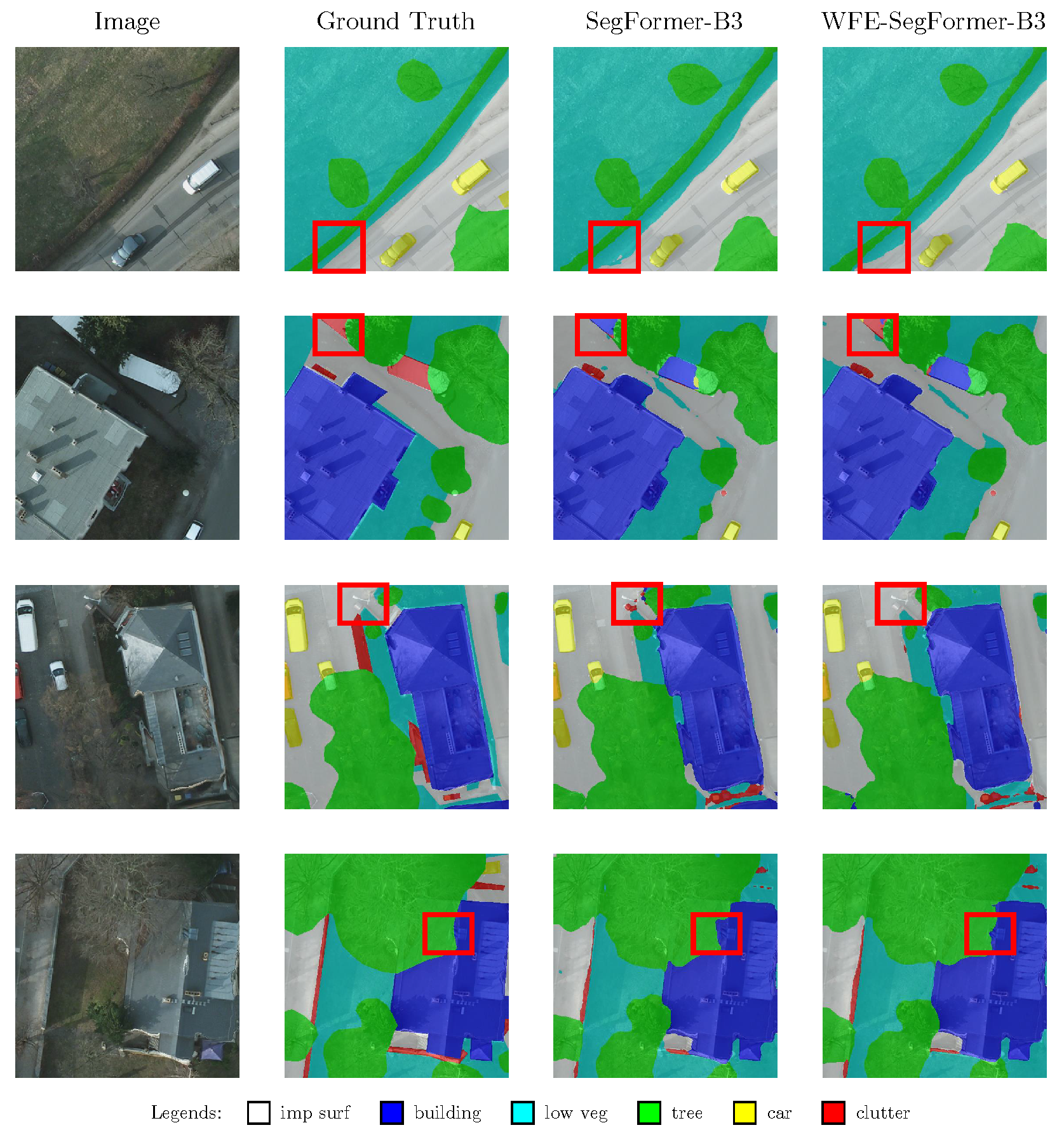
Figure 6. In our research, we have discovered that our module is more effective in detecting borders of large objects surrounding buildings and trees, as demonstrated in
Figure 5 and
Figure 6. However, our module struggles with identifying small clusters of pixels and fine details. This is due to its sensitivity towards high frequency information around large objects, rather than small objects or near the edge of the image. Additionally,
Figure 4 presents the curve of OA against epochs during the training process, indicating that adopting our module results in faster convergence throughout the training process.
4.3. Experiments on ISPRS Vaihingen
This section introduces our experiment conducted on ISPRS Vaihingen.
4.3.1. ISPRS Vaihingen Dataset
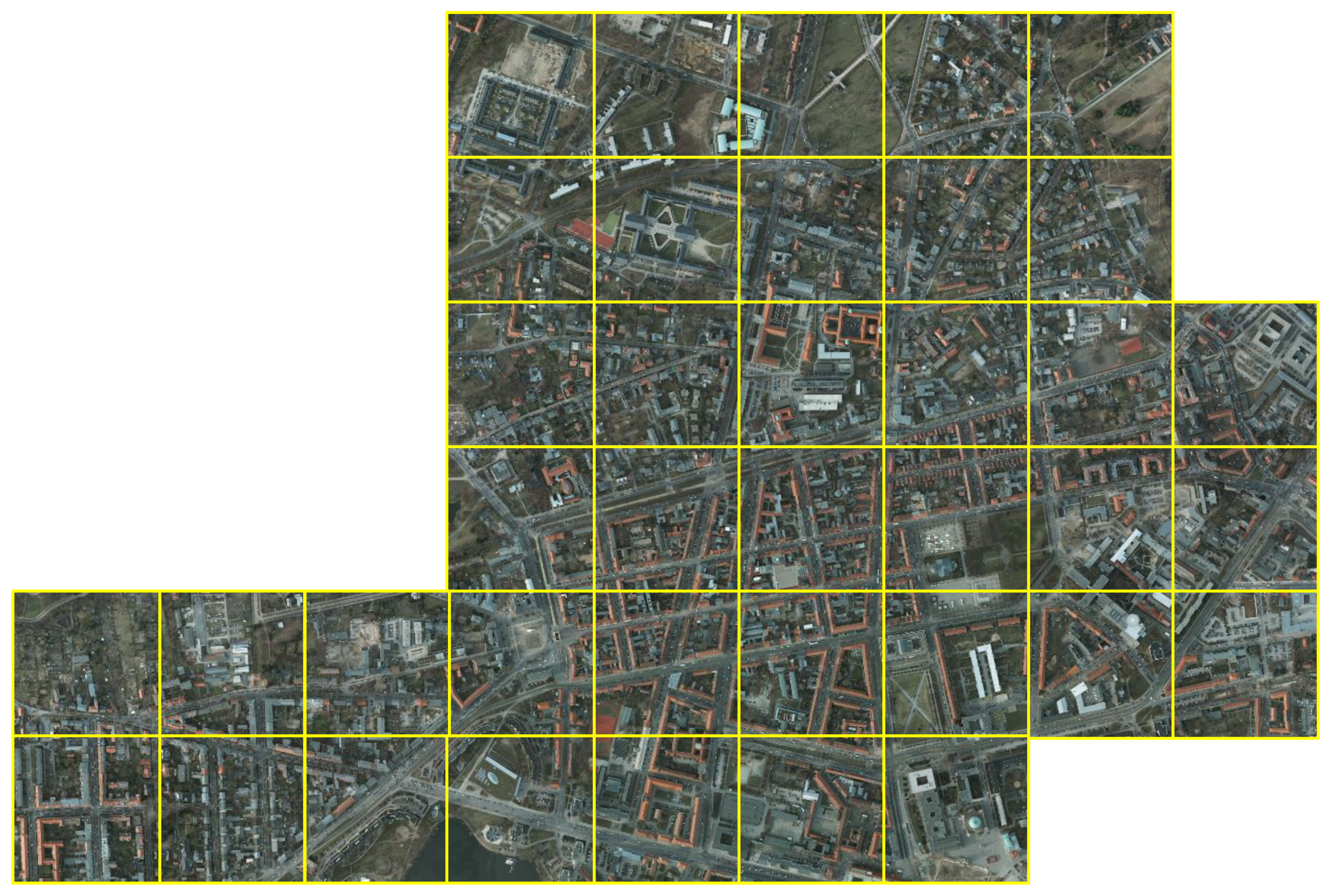
The ISPRS Vaihingen dataset, shown in
Figure 7, is also a well-known dataset for semantic segmentation of RSI. It contains 33 ortho-rectified images of the city of Vaihingen, Germany, with a spatial resolution of 9 cm. All images are of different sizes, ranging from
pixels to
pixels. The images are divided into 16 and 17 images for training and validation, respectively. Like the ISPRS Potsdam dataset, the images are annotated with six classes: impervious surfaces (imp surf), building, low vegetation (low veg), tree, car, and clutter.
During the training, we crop the images to pixels (allow overlapping at the edges), and randomly flip the images horizontally and vertically, thus producing 344 images for training and 398 images for validation.
4.3.2. Experimental Settings on ISPRS Vaihingen
Similar to the experiments on the ISPRS Potsdam dataset, we conduct experiments on the ISPRS Vaihingen dataset. Due to the smaller dataset, we selected fewer models with moderate sizes to validate our method’s efficiency and effectiveness.
4.3.3. Results on ISPRS Vaihingen
Based on the results presented in
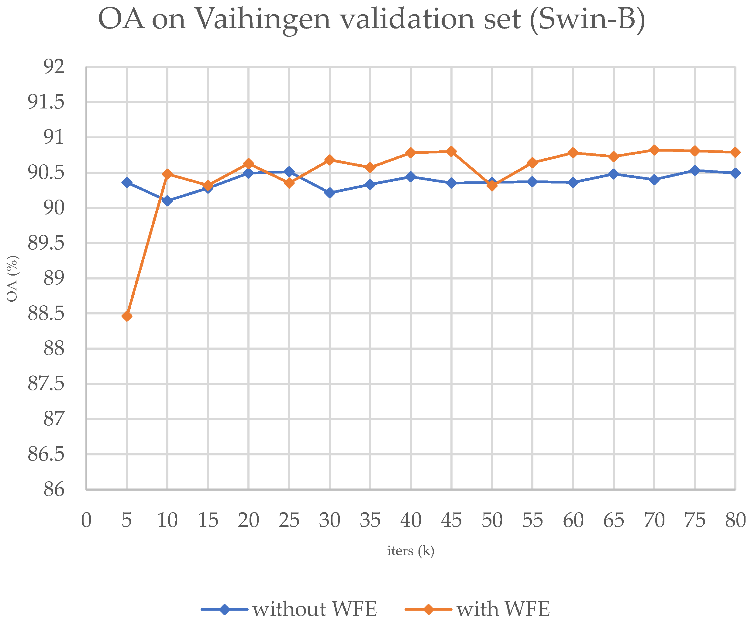
Table 2, it is evident that the performance of the original models that are based on transformers has improved by approximately 0.3% after the adoption of the WFE module. The improvement on the CNNs is also competitive. Also, we present the training OA curve in
Figure 8 and the sample results in
Figure 9.
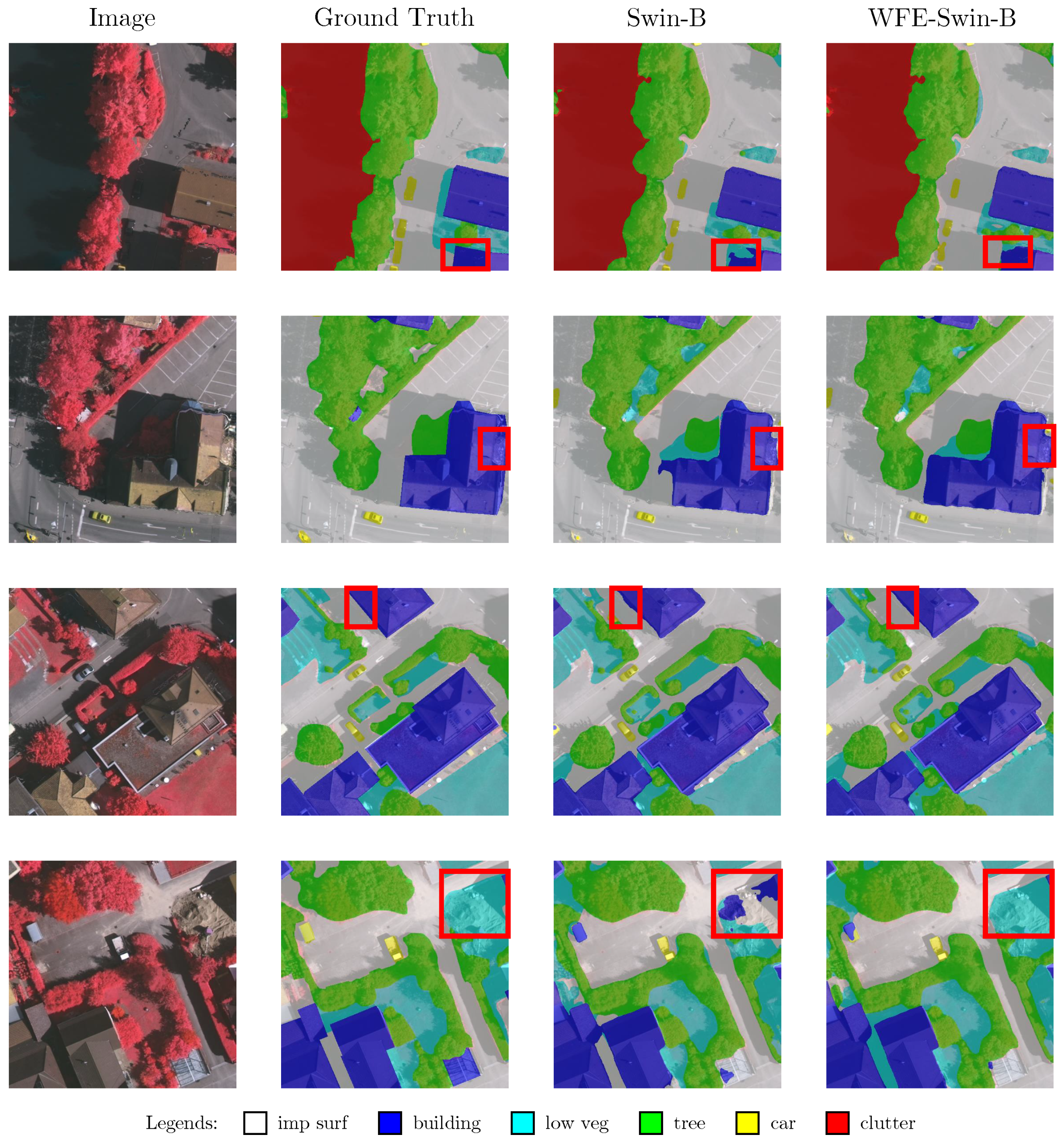
Figure 9 demonstrates that our module is superior at identifying fine details, which is consistent with the results obtained on the ISPRS Potsdam dataset where small clusters of pixels are better categorized. Additionally, an OA curve of the training process has been provided, which showcases the superior ability of our module.
It is worth noting that our module has a better improvement on transformers than on CNNs when compared to the larger dataset, i.e., Potsdam. However, in smaller datasets like Vaihingen, the generalization potential of the WFE module is largely affected, resulting in little advantage or even disadvantage over CNN-based frameworks.
4.4. Ablation Studies
In the ablation studies, we use SegFormer and UPerNet as the baseline model and conduct experiments on the ISPRS Potsdam dataset to evaluate the effectiveness and efficiency of different settings of our method. The results are displayed in
Table 3.
4.4.1. Diagonal Initialization
For the WFE module, we use a diagonal initialization method in order to ensure that the wavelet blocks do not change the features extracted by the convolutional layers initially, so as to ensure the stability of the training process.
To verify the effectiveness of the diagonal initialization method, we conducted experiments on the ISPRS Potsdam dataset, with and without the diagonal initialization method. The results are shown in
Table 3, groups #1 and #2. From the results, we can see that the diagonal initialization method can improve the performance of the original model substantially. This proves the diagonal initialization method to be effective.
The adoption of diagonal initialization is essential in our method, as it eliminates the need to pre-train. The current procedure is similar to training the enhanced model from the unenhanced model by parameter freezing, but with added coupling between relevant parameters.
4.4.2. Number of Channels
In our WFE module, we can control whether to use grayscale or RGB images as the input of the 2D-DWT. To verify its effect, we conducted experiments on the ISPRS Potsdam dataset, with grayscale and RGB images as the input of the 2D-DWT, respectively. The results are shown in
Table 3, groups #2 and #3. From the results, we can see that the performance of the original model reaches its peak when RGB images are used as the input of the 2D-DWT. This proves that the RGB images contain more information than grayscale images, and thus can improve the performance.
4.4.3. Frequency Components Fed into the Backbone
For the WFE module, we can control the number of frequency maps out of the 2D-DWT to be fed to the backbone. To verify its effect, we conducted experiments on the ISPRS Potsdam dataset, with different frequency components fed into the backbone. The results are shown in
Table 3, groups #3 through #5. From the results, we can see that the performance of the original model reaches its peak when all the frequency components are fed into the backbone. This proves that the WFE module can extract useful information from the frequency components, and feed them to the backbone to enhance the features.
4.4.4. Maximum Pooling
Due to the nonexistence of the 1/2 resolution feature maps in the original SegFormer, we tried to use maximum pooling to downsample the full resolution feature maps to 1/2 resolution before applying the 2D-DWT to the downsampled feature maps. The results are shown in
Table 3, group #6. From the results, we can see that the performance of the WFE model drops when maximum pooling takes place. This is possibly because the maximum pooling operation loses the positional information of the features, leading to the 2D-DWT not being able to extract useful information from the downsampled feature maps.
4.4.5. Skip Connection
In semantic segmentation tasks, the encoder are linked to the decoder by an output and multiple skip connections. In an experiment on ConvNeXt-B, we performed multiple groups of comparisons, and found out that injecting the WFE branch back right before skip connections marginally outperforms the result of injecting them right after the skip connections. This shows that WFE block is stable and would never pose structurally destructive consequences on the decoder.
4.4.6. Type of Transform
In our related works, we conducted a review of various transforms including DFT and DCT. To compare the outcomes of DWT with those of DFT and DCT, we conducted an experiment. We derived the DFT and DCT branches from the input image by first interpolating it to the same size as the main branch. We then performed DFT or DCT, followed by a linear layer and finally the inverse transform. We fused it into the main branch using
convolution. The results are tabulated in
Table 4. The experiment showed that DWT (#4) significantly outperforms DFT (#7) and DCT (#8). We attribute this difference to the inherent hierarchy property of the discrete wavelet transform and the lower parameter count with the elimination of the linear layer. Note that both the DFT and DCT groups (#7, #8) exhibit weaker performance than the original ResNet. This suggests that excessive information has been injected into the framework, leading to overfitting.
5. Discussions
Based on our experiments, here we analyze our results and present our discussion.
Our module is a generalized model, which can be implemented on a wide range of hierarchical encoder–decoder architectures, improving the results.
The main reason we introduce 2D-DWT as a module is because of its property of being lossless. In essence, 2D-DWT can be regarded as a downsampling operation, with information from the previous layers preserved, to supplement the model with the original information.
Our module has the following merits:
The WFE module is a hierarchical module, which can be applied to the CNNs and transformers to enhance the features.
The WFE module is a lightweight module, which can be generalized to different models, and can improve the performance of the original models in the context of remote sensing images, with little additional computation.
The WFE module is a general module, which can be applied to different models, and can be used on different tasks.
Still, our module has some limitations that can be improved upon:
During the segmentation, our module can make little improvements at the edge of the entire image.
Our module has different adaptability towards architectures of different sizes. The WFE module generally better adapts to small- or mid-sized models.
Our module performed better on models when a WFE module can be injected in the stem layer makes a difference, because the wavelet block 0 has a relatively larger perception field.
6. Conclusions
We have introduced a new technique, known as Hierarchical Wavelet Feature Enhancement (WFE), in this paper to enhance the features of CNNs and transformers. We conducted experiments and analyzed our approach to demonstrate its usefulness and versatility. Going forward, we plan to apply the WFE module to different models and tasks to further validate its effectiveness and efficiency. Additionally, we will keep track of the latest state-of-the-art models, upgrades, and patches to traditional models and continue using our methods to better assess the universality and adaptability of our module.
Author Contributions
Conceptualization, J.Y. and H.Z.; Formal analysis, Y.L. and Z.L.; Funding acquisition, J.Y. and H.Z.; Methodology, Y.L. and Z.L.; Project administration, J.Y. and H.Z.; Resources, J.Y. and H.Z.; Software, Y.L. and Z.L.; Supervision, J.Y. and H.Z.; Validation, J.Y. and H.Z.; Visualization, Y.L. and Z.L.; Writing—original draft preparation, Y.L. and Z.L.; Writing—review and editing, J.Y. and H.Z. All authors have read and agreed to the published version of the manuscript.
Funding
This work was supported in part by the National Natural Science Foundation of China (Grant No. 62271018), and the Beijing University Student Innovation and Entrepreneurship Training Intercollegiate Cooperation Program (Grant No. 202298066).
Data Availability Statement
Conflicts of Interest
The authors declare no conflict of interest. The funders had no role in the design of the study; in the collection, analyses, or interpretation of data; in the writing of the manuscript; or in the decision to publish the results.
Abbreviations
The following abbreviations are used in this manuscript:
| WFE | Wavelet Feature Enhancement Module |
| ISPRS | International Society for Photogrammetry and Remote Sensing |
| DWT | discrete wavelet transform |
| DFT | discrete Fourier transform |
| DCT | discrete Cosine transform |
| CNN | convolutional neural network |
| FCN | fully convolutional network |
| OA | overall accuracy |
| mIoU | mean intersection over union |
| mF1 | mean F1 score |
References
- Long, J.; Shelhamer, E.; Darrell, T. Fully convolutional networks for semantic segmentation. In Proceedings of the 2015 IEEE Conference on Computer Vision and Pattern Recognition (CVPR), Boston, MA, USA, 7–12 June 2015; pp. 3431–3440. [Google Scholar] [CrossRef]
- Zhao, H.; Shi, J.; Qi, X.; Wang, X.; Jia, J. Pyramid Scene Parsing Network. In Proceedings of the 2017 IEEE Conference on Computer Vision and Pattern Recognition (CVPR), Honolulu, HI, USA, 21–26 July 2017; pp. 6230–6239. [Google Scholar] [CrossRef]
- Wu, H.; Zhang, J.; Huang, K.; Liang, K.; Yu, Y. FastFCN: Rethinking Dilated Convolution in the Backbone for Semantic Segmentation. arXiv 2019, arXiv:1706.05587. [Google Scholar] [CrossRef]
- Chen, L.C.; Papandreou, G.; Schroff, F.; Adam, H. Rethinking Atrous Convolution for Semantic Image Segmentation. arXiv 2017, arXiv:1706.05587. [Google Scholar] [CrossRef]
- Xiao, T.; Liu, Y.; Zhou, B.; Jiang, Y.; Sun, J. Unified Perceptual Parsing for Scene Understanding. In Proceedings of the Computer Vision—ECCV 2018: 15th European Conference, Munich, Germany, 8–14 September 2018; Proceedings, Part V. Springer: Cham, Switzerland, 2018; pp. 432–448. [Google Scholar] [CrossRef]
- Liu, Z.; Mao, H.; Wu, C.Y.; Feichtenhofer, C.; Darrell, T.; Xie, S. A ConvNet for the 2020s. In Proceedings of the 2022 IEEE/CVF Conference on Computer Vision and Pattern Recognition (CVPR), New Orleans, LA, USA, 18–24 June 2022; pp. 11966–11976. [Google Scholar] [CrossRef]
- Rao, Y.; Zhao, W.; Tang, Y.; Zhou, J.; Lim, S.N.; Lu, J. HorNet: Efficient High-Order Spatial Interactions with Recursive Gated Convolutions. In Proceedings of the Advances in Neural Information Processing Systems, New Orleans, LA, USA, 28 November–9 December 2022; Volume 35, pp. 10353–10366. [Google Scholar]
- Wang, W.; Dai, J.; Chen, Z.; Huang, Z.; Li, Z.; Zhu, X.; Hu, X.; Lu, T.; Lu, L.; Li, H.; et al. InternImage: Exploring Large-Scale Vision Foundation Models With Deformable Convolutions. In Proceedings of the IEEE/CVF Conference on Computer Vision and Pattern Recognition (CVPR), Vancouver, BC, Canada, 18–22 June 2023; pp. 14408–14419. [Google Scholar]
- Vaswani, A.; Shazeer, N.; Parmar, N.; Uszkoreit, J.; Jones, L.; Gomez, A.N.; Kaiser, L.; Polosukhin, I. Attention is All You Need. In Proceedings of the 31st International Conference on Neural Information Processing Systems, Long Beach, CA, USA, 4–9 December 2017; pp. 6000–6010. [Google Scholar]
- Dosovitskiy, A.; Beyer, L.; Kolesnikov, A.; Weissenborn, D.; Zhai, X.; Unterthiner, T.; Dehghani, M.; Minderer, M.; Heigold, G.; Gelly, S.; et al. An Image is Worth 16x16 Words: Transformers for Image Recognition at Scale. In Proceedings of the International Conference on Learning Representations, Virtual, 3–7 May 2021. [Google Scholar]
- Xie, E.; Wang, W.; Yu, Z.; Anandkumar, A.; Alvarez, J.M.; Luo, P. SegFormer: Simple and Efficient Design for Semantic Segmentation with Transformers. In Proceedings of the Advances in Neural Information Processing Systems, Online, 6–14 December 2021; Volume 34, pp. 12077–12090. [Google Scholar]
- Liu, Z.; Lin, Y.; Cao, Y.; Hu, H.; Wei, Y.; Zhang, Z.; Lin, S.; Guo, B. Swin Transformer: Hierarchical Vision Transformer Using Shifted Windows. In Proceedings of the ICCV 2021, Virtual, 11–17 October 2021. [Google Scholar]
- Xia, Z.; Pan, X.; Song, S.; Li, L.E.; Huang, G. Vision Transformer with Deformable Attention. In Proceedings of the 2022 IEEE/CVF Conference on Computer Vision and Pattern Recognition (CVPR), New Orleans, LA, USA, 18–24 June 2022; pp. 4784–4793. [Google Scholar] [CrossRef]
- Bai, L.; Lin, X.; Ye, Z.; Xue, D.; Yao, C.; Hui, M. MsanlfNet: Semantic Segmentation Network With Multiscale Attention and Nonlocal Filters for High-Resolution Remote Sensing Images. IEEE Geosci. Remote Sens. Lett. 2022, 19, 6512405. [Google Scholar] [CrossRef]
- Jia, S.; Yao, W. Joint learning of frequency and spatial domains for dense image prediction. ISPRS J. Photogramm. Remote Sens. 2023, 195, 14–28. [Google Scholar] [CrossRef]
- Zhang, Y.; Gao, X.; Duan, Q.; Leng, J.; Pu, X.; Gao, X. Contextual Learning in Fourier Complex Field for VHR Remote Sensing Images. arXiv 2022, arXiv:2210.15972. [Google Scholar] [CrossRef] [PubMed]
- Tang, W.; Shakeel, M.S.; Chen, Z.; Wan, H.; Kang, W. Target Category Agnostic Knowledge Distillation With Frequency-Domain Supervision. IEEE Trans. Ind. Inform. 2023, 19, 8462–8471. [Google Scholar] [CrossRef]
- Bo, D.; Pichao, W.; Wang, F. AFFormer: Head-Free Lightweight Semantic Segmentation with Linear Transformer. AAAI Conf. Artif. Intell. 2023, 37, 516–524. [Google Scholar] [CrossRef]
- Lo, S.Y.; Hang, H.M. Exploring Semantic Segmentation on the DCT Representation. In Proceedings of the ACM Multimedia Asia, Beijing, China, 15–18 December 2020. [Google Scholar] [CrossRef]
- Huang, J.; Guan, D.; Xiao, A.; Lu, S. FSDR: Frequency Space Domain Randomization for Domain Generalization. In Proceedings of the 2021 IEEE/CVF Conference on Computer Vision and Pattern Recognition (CVPR), Nashville, TN, USA, 19–25 June 2021; pp. 6887–6898. [Google Scholar] [CrossRef]
- Pan, H.; Zhu, X.; Atici, S.; Cetin, A.E. DCT Perceptron Layer: A Transform Domain Approach for Convolution Layer. arXiv 2017, arXiv:2211.08577. [Google Scholar] [CrossRef]
- Liu, P.; Zhang, H.; Lian, W.; Zuo, W. Multi-Level Wavelet Convolutional Neural Networks. IEEE Access 2019, 7, 74973–74985. [Google Scholar] [CrossRef]
- Li, Q.; Shen, L. WaveSNet: Wavelet Integrated Deep Networks for Image Segmentation. In Proceedings of the Pattern Recognition and Computer Vision, Shenzhen, China, 14–17 October 2022; pp. 325–337. [Google Scholar] [CrossRef]
- Su, Y.C.; Liu, T.J.; Liuy, K.H. Multi-scale Wavelet Frequency Channel Attention for Remote Sensing Image Segmentation. In Proceedings of the 2022 IEEE 14th Image, Video, and Multidimensional Signal Processing Workshop (IVMSP), Nafplio, Greece, 26–29 June 2022; pp. 1–5. [Google Scholar] [CrossRef]
- Azimi, S.M.; Fischer, P.; Körner, M.; Reinartz, P. Aerial LaneNet: Lane-Marking Semantic Segmentation in Aerial Imagery Using Wavelet-Enhanced Cost-Sensitive Symmetric Fully Convolutional Neural Networks. IEEE Trans. Geosci. Remote Sens. 2019, 57, 2920–2938. [Google Scholar] [CrossRef]
- Yao, T.; Pan, Y.; Li, Y.; Ngo, C.W.; Mei, T. Wave-ViT: Unifying Wavelet and Transformers for Visual Representation Learning. In Proceedings of the Computer Vision—ECCV 2022, Tel Aviv, Israel, 23–27 October 2022; pp. 328–345. [Google Scholar] [CrossRef]
- Zhang, Z.; Liu, F.; Liu, C.; Tian, Q.; Qu, H. ACTNet: A Dual-Attention Adapter with a CNN-Transformer Network for the Semantic Segmentation of Remote Sensing Imagery. Remote Sens. 2023, 15, 2363. [Google Scholar] [CrossRef]
- Cheng, B.; Misra, I.; Schwing, A.G.; Kirillov, A.; Girdhar, R. Masked-attention Mask Transformer for Universal Image Segmentation. In Proceedings of the 2022 IEEE/CVF Conference on Computer Vision and Pattern Recognition (CVPR), New Orleans, LA, USA, 18–24 June 2022; pp. 1280–1289. [Google Scholar] [CrossRef]
- Chen, X.; Li, D.; Liu, M.; Jia, J. CNN and Transformer Fusion for Remote Sensing Image Semantic Segmentation. Remote Sens. 2023, 15, 4455. [Google Scholar] [CrossRef]
- Zhang, X.; Li, L.; Di, D.; Wang, J.; Chen, G.; Jing, W.; Emam, M. SERNet: Squeeze and Excitation Residual Network for Semantic Segmentation of High-Resolution Remote Sensing Images. Remote Sens. 2022, 14, 4770. [Google Scholar] [CrossRef]
- Hu, J.; Shen, L.; Sun, G. Squeeze-and-Excitation Networks. In Proceedings of the 2018 IEEE/CVF Conference on Computer Vision and Pattern Recognition, Salt Lake City, UT, USA, 18–23 June 2018; pp. 7132–7141. [Google Scholar] [CrossRef]
- Fang, L.; Zhou, P.; Liu, X.; Ghamisi, P.; Chen, S. Context Enhancing Representation for Semantic Segmentation in Remote Sensing Images. IEEE Trans. Neural Netw. Learn. Syst. 2022; early access. [Google Scholar] [CrossRef]
- Yang, Y.; Soatto, S. FDA: Fourier Domain Adaptation for Semantic Segmentation. In Proceedings of the 2020 IEEE/CVF Conference on Computer Vision and Pattern Recognition (CVPR), Seattle, WA, USA, 14–19 June 2020; pp. 4084–4094. [Google Scholar] [CrossRef]
- He, K.; Zhang, X.; Ren, S.; Sun, J. Deep Residual Learning for Image Recognition. In Proceedings of the IEEE Conference on Computer Vision and Pattern Recognition (CVPR), Las Vegas, NV, USA, 27–30 June 2016; pp. 770–778. [Google Scholar] [CrossRef]
- Paszke, A.; Gross, S.; Massa, F.; Lerer, A.; Bradbury, J.; Chanan, G.; Killeen, T.; Lin, Z.; Gimelshein, N.; Antiga, L.; et al. PyTorch: An Imperative Style, High-Performance Deep Learning Library. In Proceedings of the 33rd International Conference on Neural Information Processing Systems, Vancouver, BC, Canada, 8–14 December 2019; pp. 8024–8035. [Google Scholar]
Figure 1.
The 2D-DWT diagram is shown in two sub-figures. Sub-figure (a) demonstrates the 2D-DWT procedure, with downsampling represented by a down-arrow. Sub-figure (b) displays the hierarchy of 2D-DWT, with the figure showing the resolutions of each component.
Figure 1.
The 2D-DWT diagram is shown in two sub-figures. Sub-figure (a) demonstrates the 2D-DWT procedure, with downsampling represented by a down-arrow. Sub-figure (b) displays the hierarchy of 2D-DWT, with the figure showing the resolutions of each component.
Figure 2.
The diagrams illustrate the main procedures in and around the WFE module. Sub-figure (a) is based on the UPerNet−ResNet50 framework, and sub-figure (b) depicts the working principle of our Wavelet block.
Figure 2.
The diagrams illustrate the main procedures in and around the WFE module. Sub-figure (a) is based on the UPerNet−ResNet50 framework, and sub-figure (b) depicts the working principle of our Wavelet block.
Figure 3.
ISPRS Potsdam dataset sample.
Figure 3.
ISPRS Potsdam dataset sample.
Figure 4.
The OA curve on the validation set during the training process on ISPRS Potsdam, with SegFormer-B3.
Figure 4.
The OA curve on the validation set during the training process on ISPRS Potsdam, with SegFormer-B3.
Figure 5.
Sample results with SegFormer-B3 (representing the results on transformers) include comparisons with and without WFE. The red rectangles mark the improvement of the WFE version against the original architecture.
Figure 5.
Sample results with SegFormer-B3 (representing the results on transformers) include comparisons with and without WFE. The red rectangles mark the improvement of the WFE version against the original architecture.
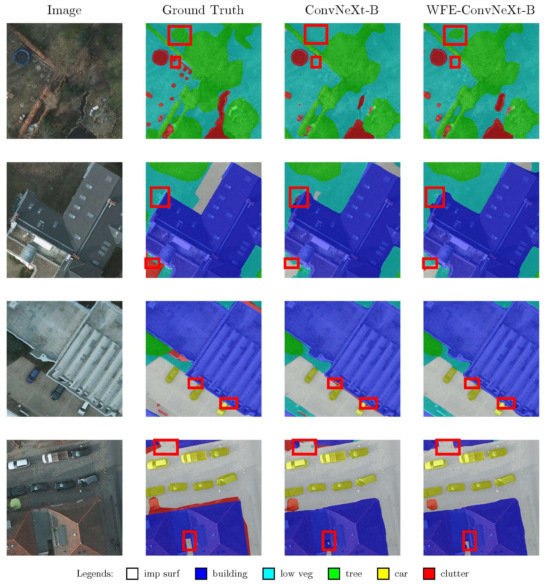
Figure 6.
Sample results with ConvNeXt-B (representing the results on CNNs) include comparisons with and without WFE. The red rectangles mark the improvement of the WFE version against the original architecture. Note: The ground truths shown above are not border-eroded, whereas the models were trained and validated on the border-eroded version of the ground truth.
Figure 7.
ISPRS Vaihingen dataset sample.
Figure 7.
ISPRS Vaihingen dataset sample.
Figure 8.
The OA curve on the validation set during the training process on ISPRS Vaihingen, with Swin-B.
Figure 8.
The OA curve on the validation set during the training process on ISPRS Vaihingen, with Swin-B.
Figure 9.
Sample results with Swin-B include comparisons with and without WFE. Note: The ground truths shown above are not border-eroded, whereas the models were trained and validated on the border-eroded version of the ground truth.
Figure 9.
Sample results with Swin-B include comparisons with and without WFE. Note: The ground truths shown above are not border-eroded, whereas the models were trained and validated on the border-eroded version of the ground truth.
Table 1.
Experiments on ISPRS Potsdam. Shows the OA, mIoU, mF1, and Class Acc of our method on the ISPRS Potsdam dataset. The OA and the mIoU include the clutter class, whereas the mF1 and the Class Acc exclude it. The results of the original models are also listed for comparison; bold indicates the best.
| Method | Backbone | WFE | OA | mIoU | mF1 | Class Acc |
|---|
| Imp Surf | Building | Low Veg | Tree | Car |
|---|
| Transformers |
| UPerNet | Swin-T | − | 91.02 | 78.47 | 92.45 | 93.94 | 97.72 | 89.37 | 88.73 | 95.66 |
| + | 91.03 | 78.68 | 92.50 | 94.08 | 97.38 | 89.76 | 87.92 | 95.24 |
| UPerNet | Swin-S | − | 91.13 | 78.98 | 92.07 | 94.00 | 97.53 | 91.01 | 87.16 | 96.26 |
| + | 91.20 | 79.05 | 92.64 | 94.23 | 97.44 | 89.78 | 88.52 | 95.47 |
| UPerNet | Swin-B | − | 91.29 | 79.40 | 92.70 | 94.01 | 97.74 | 90.16 | 88.05 | 96.70 |
| + | 91.37 | 79.50 | 92.85 | 94.40 | 97.55 | 90.23 | 88.11 | 96.59 |
| SegFormer | MiT-b4 | − | 91.13 | 78.79 | 92.60 | 94.32 | 97.71 | 91.06 | 86.78 | 96.41 |
| + | 91.38 | 79.50 | 92.69 | 94.32 | 97.42 | 90.04 | 88.85 | 96.39 |
| SegFormer | MiT-b3 | − | 91.20 | 78.94 | 92.61 | 93.55 | 96.97 | 87.65 | 88.91 | 95.97 |
| + | 91.42 | 79.67 | 92.71 | 93.80 | 97.14 | 87.64 | 89.04 | 95.95 |
| CNNs |
| UPerNet | InternImage-B | − | 91.37 | 79.60 | 92.93 | 94.23 | 97.85 | 90.40 | 88.74 | 96.12 |
| + | 91.44 | 79.65 | 92.87 | 94.06 | 97.88 | 88.09 | 91.25 | 96.29 |
| UPerNet | ConvNeXt-S | − | 91.21 | 79.30 | 92.69 | 94.12 | 97.57 | 90.41 | 87.63 | 96.41 |
| + | 91.22 | 79.12 | 92.60 | 94.11 | 97.70 | 90.42 | 87.13 | 96.70 |
| UPerNet | ConvNeXt-B | − | 91.34 | 79.44 | 92.69 | 94.56 | 97.48 | 89.48 | 88.80 | 96.10 |
| + | 91.36 | 79.48 | 92.69 | 94.32 | 97.15 | 88.75 | 89.89 | 96.79 |
| UPerNet | ResNet-50 | − | 90.06 | 77.23 | 91.58 | 92.42 | 96.96 | 89.26 | 86.46 | 95.32 |
| + | 90.54 | 78.27 | 92.00 | 93.20 | 96.85 | 89.70 | 86.57 | 95.07 |
| UPerNet | ResNet-101 | − | 89.85 | 77.13 | 91.30 | 92.01 | 96.28 | 89.31 | 84.92 | 94.37 |
| + | 90.01 | 77.32 | 91.37 | 92.48 | 96.63 | 89.89 | 85.61 | 94.39 |
| DeepLabV3+ | ResNet-50 | − | 88.97 | 74.00 | 89.21 | 91.20 | 96.31 | 88.61 | 84.77 | 85.32 |
| + | 89.14 | 74.01 | 89.23 | 90.93 | 95.93 | 89.64 | 86.26 | 84.30 |
Table 2.
Experiments on ISPRS Vaihingen. Shows the OA, mIoU, mF1, and Class Acc of our method on the ISPRS Vaihingen dataset, with results of the original models also listed for comparison. The OA and the mIoU include the clutter class, whereas the mF1 and the Class Acc exclude it. Bold indicates the best.
| Method | Backbone | WFE | OA | mIoU | mF1 | Class Acc |
|---|
| Imp Surf | Building | Low Veg | Tree | Car |
|---|
| Transformers |
| UPerNet | Swin-B | − | 90.53 | 73.19 | 89.58 | 93.64 | 96.20 | 81.52 | 91.52 | 84.83 |
| + | 90.89 | 74.45 | 89.82 | 92.89 | 96.82 | 81.75 | 92.68 | 85.01 |
| SegFormer | MiT-b3 | − | 90.65 | 74.35 | 89.95 | 92.69 | 95.94 | 84.03 | 89.39 | 87.72 |
| + | 90.66 | 74.08 | 89.95 | 92.77 | 95.94 | 84.07 | 89.35 | 87.61 |
| CNNs |
| UPerNet | InternImage-S | − | 90.86 | 74.52 | 90.17 | 93.64 | 96.31 | 81.88 | 92.10 | 87.04 |
| + | 90.89 | 73.71 | 90.10 | 93.59 | 96.34 | 82.35 | 91.92 | 87.88 |
| UPerNet | ConvNeXt-S | − | 90.84 | 74.04 | 90.08 | 93.25 | 96.28 | 83.21 | 91.37 | 86.69 |
| + | 90.73 | 73.67 | 89.94 | 93.35 | 96.32 | 82.04 | 91.89 | 86.55 |
| UPerNet | ResNet-50 | − | 89.74 | 69.88 | 88.26 | 91.80 | 94.98 | 83.35 | 88.73 | 82.44 |
| + | 89.58 | 70.20 | 88.46 | 91.94 | 94.91 | 82.70 | 88.50 | 84.27 |
Table 3.
Ablation studies on ISPRS Potsdam. The diagonal column indicates whether diagonal initialization is applied, whereas the gray column stands for whether gray-scaling is performed. In the levels column, H stands for HH, HL, and LH sub-bands, and L stands for the LL sub-band. In the pooling column, avg stands for average pooling and max stands for maximum pooling. Bold indicates the best.
| # | Method | Backbone | Diagonal | Gray | Levels | Pooling | OA | mIoU |
|---|
| 0 | SegFormer | MiT-b4 | — | 91.13 | 78.79 |
| 1 | SegFormer | WFE-MiT-b4 | − | + | H | Avg | 90.18 | 76.94 |
| 2 | + | + | H | Avg | 91.16 | 78.80 |
| 3 | + | − | H | Avg | 91.22 | 79.09 |
| 4 | + | − | L | Avg | 91.23 | 79.08 |
| 5 | + | − | L and H | Avg | 91.38 | 79.50 |
| 6 | + | − | L and H | Max | 91.27 | 79.01 |
| 0 | UPerNet | ResNet50 | — | 90.06 | 77.23 |
| 1 | UPerNet | WFE-ResNet50 | − | + | H | Avg | 90.08 | 77.62 |
| 2 | + | + | H | Avg | 90.17 | 77.96 |
| 3 | + | − | H | Avg | 90.31 | 78.18 |
| 4 | + | − | L | Avg | 90.43 | 77.57 |
| 5 | + | − | L and H | Avg | 90.54 | 78.27 |
| 6 | + | − | L and H | Max | 90.39 | 78.21 |
Table 4.
Ablation studies on ISPRS Potsdam, comparing DCT and DFT with our proposed DWT architecture. Bold indicates the best.
Table 4.
Ablation studies on ISPRS Potsdam, comparing DCT and DFT with our proposed DWT architecture. Bold indicates the best.
| # | Method | Backbone | Transform Type | OA | mIoU |
|---|
| 0 | UPerNet | WFE-ResNet | DWT | 90.06 | 77.23 |
| 4 | UPerNet | WFE-ResNet | DWT | 90.54 | 78.27 |
| 7 | UPerNet | WFE-ResNet | DFT | 88.39 | 73.75 |
| 8 | UPerNet | WFE-ResNet | DCT | 87.86 | 72.29 |
| Disclaimer/Publisher’s Note: The statements, opinions and data contained in all publications are solely those of the individual author(s) and contributor(s) and not of MDPI and/or the editor(s). MDPI and/or the editor(s) disclaim responsibility for any injury to people or property resulting from any ideas, methods, instructions or products referred to in the content. |
© 2023 by the authors. Licensee MDPI, Basel, Switzerland. This article is an open access article distributed under the terms and conditions of the Creative Commons Attribution (CC BY) license (https://creativecommons.org/licenses/by/4.0/).


