YOLO-RS: A More Accurate and Faster Object Detection Method for Remote Sensing Images

Abstract

In recent years, object detection based on deep learning has been widely applied and developed. When using object detection methods to process remote sensing images, the trade-off between the speed and accuracy of models is necessary, because remote sensing images pose additional difficulties such as complex backgrounds, small objects, and dense distribution to the detection task. This paper proposes YOLO-RS, an optimized object detection algorithm based on YOLOv4 to address the challenges. The Adaptively Spatial Feature Fusion (ASFF) structure is introduced after the feature enhancement network of YOLOv4. It assigns adaptive weight parameters to fuse multi-scale feature information, improving detection accuracy. Furthermore, optimizations are applied to the Spatial Pyramid Pooling (SPP) structure in YOLOv4. By incorporating residual connections and employing 1 × 1 convolutions after maximum pooling, both computation complexity and detection accuracy are improved. To enhance detection speed, Lightnet is introduced, inspired by Depthwise Separable Convolution for reducing model complexity. Additionally, the loss function in YOLOv4 is optimized by introducing the Intersection over Union loss function. This change replaces the aspect ratio loss term with the edge length loss, enhancing sensitivity to width and height, accelerating model convergence, and improving regression accuracy for detected frames. The mean Average Precision (mAP) values of the YOLO-RS model are 87.73% and 92.81% under the TGRS-HRRSD dataset and RSOD dataset, respectively, which are experimentally verified to be 2.15% and 1.66% higher compared to the original YOLOv4 algorithm. The detection speed reached 43.45 FPS and 43.68 FPS, respectively, with 5.29 Frames Per Second (FPS) and 5.30 FPS improvement.

1. Introduction

In recent years, remote sensing technology has rapidly developed and its applications have become increasingly diverse in various fields [1,2,3,4], playing an important role in military, civilian, and other fields. It is an important foundation for applications such as urban planning, land use, and natural disaster monitoring.

Remote sensing image object detection is one of the most fundamental tasks in satellite remote sensing image processing, which refers to the use of image processing technology and relevant computer vision algorithms to determine whether there are target objects in the acquired remote sensing image. Therefore, how to improve the performance of remote sensing image object detection to obtain more accurate positioning and detailed classification recognition has become one of the important research topics in the field of remote sensing. In traditional feature-based object detection methods, candidate regions are first extracted from the image, and then handcrafted features are designed for the detected objects. Finally, a classifier is used to perform the detection task. However, due to the high resolution and large data volume of remote sensing images, as well as the limitations of handcrafted feature descriptors in representing diverse features, traditional object detection algorithms fail to fully exploit the deep semantic information in remote sensing images, resulting in low efficiency and high computational costs. In recent years, breakthroughs have been made in object detection using deep learning compared to traditional approaches. Deep learning-based object detection algorithms abandon the manual feature engineering process and instead select discriminative features from massive image samples using convolutional neural network structures, leading to more reliable detection results. Therefore, expanding the application of deep learning-based object detection algorithms in remote sensing image object detection can achieve more accurate and efficient detection results, as well as promote the development and application of object detection technology in remote sensing imagery.

Although the current mainstream object detection algorithms have shown excellent performance in conventional image detection tasks, their application in remote sensing images is still challenging due to the characteristics of remote sensing images themselves. The challenges faced by object detection tasks in remote sensing images can be summarized as follows. (1) Dense distribution of objects: Remote sensing images often contain large-scale and densely distributed objects, which can cause interference between objects and result in positioning errors. The occurrence of missed detection and false detection is also more likely. (2) Small objects in remote sensing images: Small objects are often present in remote sensing images, and the existing object detection algorithms already have defects in detecting small objects in conventional images. Their application in remote sensing images will further amplify this drawback. (3) Large differences in object characteristics: Remote sensing images contain rich geographic information, including multiple types of objects that can greatly vary in size and shape. Object detection algorithms are required to have high adaptability, which increases the difficulty of object detection. (4) Complex background of remote sensing images: The complex background of remote sensing images includes two aspects. One is that the scene itself is complex, and the other is that it is easily affected by noise and other unrelated factors. This can result in the background information being more prominent than the object information itself, which can also lead to missed detection and false detection in the detection task.

To address the challenges of remote sensing image object detection, this paper proposes a YOLO-RS method that improves both the accuracy and speed of object detection. Our contributions are: (1) To address the problems of small objects, dense distribution, and complex background in remote sensing images, we introduce ASFF and propose an improved SPP structure, namely the OSPP structure. (2) In order to make the model more lightweight and improve detection speed, we propose the Lightnet structure. (3) We use the EIOU loss function to accurately describe the differences between predicted and true bounding boxes.

2. Related Work

In recent years, researchers in the fields of remote sensing and computer vision have collaborated to design numerous object detection algorithms specifically for remote sensing images.

Some researchers have continued to focus on traditional methods based on classifiers. Huang et al. [5] proposed a hyperspectral remote sensing image object detection method. The method first segments the original image using an entropy rate superpixel segmentation algorithm, and then combines spectral features with radial basis kernels to generate spectral kernels. By introducing LBP features and weighted average filtering, spatial kernels are obtained within and between superpixels, effectively avoiding the loss of edge features during the extraction of superpixel information. Finally, the combined kernels are input into an SVM classifier to complete the classification task. Huang Hong et al. [6] presented a multi-scale feature-based object detection method for remote sensing images. The method extracts three types of multi-scale local features, including improved UFL-SC features, LBP features, and SIFT features, through dense sampling. The intermediate features of the image are then extracted using the visual bag-of-words model, and the classification task is performed using an SVM with a histogram intersection kernel. Zhu et al. [7,8,9] utilized traditional machine learning methods for improved image processing performance. They introduced the Large Margin Distribution-Supervised Novelty Detection (LMD-SND) model that enhances the performance of multi-class supervised novelty detection through margin distribution. Furthermore, they implemented Neighborhood Linear Discriminant Analysis (nLDA) for better performance when a class contains multiple clusters or subclasses. Finally, they improved the Support Vector Ordinal Regression (SVOR) model with the Relative Margin induced Support Vector Ordinal Regression (RMSVOR) model, which better accounts for the influence of samples close to the discriminant hyperplane during learning. Nie et al. [10] proposed a ship recognition method in complex backgrounds. They combined quaternion Fourier transform localization to construct a novel visual saliency detection method and used the GrabCut method for candidate region extraction. They also introduced rotation invariant modified LBP features for ship feature extraction and completed the classification task using SVM. However, in traditional object detection algorithms, the handcrafted feature representation and descriptor have limited capability, making it difficult to meet the requirements of complex scene object detection tasks.

However, traditional methods have their limitations. They often require significant manual effort and expertise for feature design and parameter tuning, leading to increased development costs. Additionally, these methods may lack generalizability and flexibility when dealing with diverse types of objects or scenes, necessitating adjustments and optimizations for different scenarios. In comparison, deep learning-based object detection algorithms have shown significant improvements in detection speed and accuracy, making them the current focus of research. Deep learning-based object detection algorithms can be divided into two categories: one-stage algorithms based on regression strategies and two-stage algorithms based on candidate regions. Some researchers have conducted research based on two-stage object detection algorithms. Sha et al. [11] proposed an aircraft object detection method for remote sensing images based on the Faster R-CNN network. The method obtains more comprehensive and detailed feature maps through multi-level fusion strategies and adjusts the scale of candidate regions, thereby improving object localization accuracy and reducing missed detections. Yang et al. [12] developed a landslide detection method for remote sensing imagery based on the Faster R-CNN network. They applied gamma transformation and Gaussian filtering for data augmentation, normalized the batch size to mitigate the influence on the model, and introduced the FPN structure for multi-scale feature fusion. Experimental results demonstrated significant improvement in detection accuracy. In summary, although two-stage object detection algorithms based on candidate regions exhibit excellent detection accuracy, they suffer from training and structural complexity, preventing a balance between detection speed and accuracy. On the other hand, one-stage object detection algorithms based on regression strategies eliminate the step of candidate box extraction, directly using a single neural network for object detection. Wen et al. [13] proposed an improved SSD algorithm for multi-scale object detection in remote sensing images. By introducing advanced background modeling and appropriate supervised learning strategies, they improved the performance of multi-scale object detection in remote sensing images. The algorithm was validated on the COCO dataset and achieved excellent results. Qu et al. [14] designed a YOLOv3 model with an auxiliary network to enhance the performance of object detection in remote sensing images. They employed the CBAM attention mechanism to suppress non-essential information and focus on critical information. They also used the DIOU loss function to expedite model training convergence and employed an adaptive feature fusion method to reduce inference overhead and improve detection speed. Shen et al. [15] enhanced the cross-scale detection in road object detection tasks using YOLOv3. They utilized the K-means-GIoU algorithm to create prior boxes and implemented a detection branch for small targets. Further improvements were made with the use of channel and spatial attention modules. The proposed method led to an increase in mAP value and better detection of small-scale objects

Despite the impressive performance of these methods in specific scenarios, their effectiveness may wane when balancing speed and accuracy. Moreover, it is not guaranteed that these methods will yield similar results with remote sensing images. Hence, this paper aims to find an approach that can balance detection speed and accuracy in remote sensing image datasets [16]. YOLOv4, proposed by Bochkovskiy et al. [17], is a classic method that achieves a balance between detection speed and accuracy. Therefore, this paper takes YOLOv4 as the baseline, and implements a series of improvements on it, thus enhancing its exceptional capabilities in handling remote sensing images.

3. Materials and Methods

Leveraging YOLOv4’s exemplary speed-accuracy trade-off in object detection, we adopt it as our baseline [17]. This research primarily optimizes the YOLOv4 object detection algorithm by enhancing feature fusion, incorporating lightweight model operations, and accelerating model convergence speed. Figure 1 illustrates the framework of the optimized YOLOv4, i.e., YOLO-RS, with the “ASFF”, “OSPP”, and “Lightnet” modules representing significant enhancements. Further details follow in the subsequent sections. Section 3.1 introduces the Adaptively Spatial Feature Fusion (ASFF) method [18], Section 3.2 presents the Spatial Pyramid Pooling (SPP) method, Section 3.3 unveils the novel backbone, Lightnet, and Section 3.4 discusses the optimization of the loss function.

3.1. ASFF

The YOLOv4 object detection algorithm utilizes the Path Aggregation Network (PANet) structure and the SPP structure as feature enhancement networks. These networks fuse low-level semantic information with high-level semantic information by employing a bottom-up structure to combine features extracted from three scales in the feature extraction network. Due to the significant variation in target sizes in remote sensing images, conflicts between features at different levels often dominate the feature pyramid. This inconsistency disrupts gradient computations during training and diminishes the effectiveness of the feature pyramid. To address this issue, this study introduces the ASFF structure after the PANet structure, as shown in Figure 2. The ASFF structure integrates multi-scale feature information by allocating adaptive weight parameters to different feature layers. This approach effectively improves the scale discrepancy of input features, enabling the network to adaptively focus on important information, suppress irrelevant interference, and efficiently combine critical feature information using a more effective feature fusion method. The ASFF structure enhances the network’s capability to extract image features, leading to improved detection performance across the entire network.

Figure 2 illustrates the architecture of the feature enhancement network after introducing ASFF. The specific process of feature enhancement is as follows: By employing the CSPDarknet-53 network [17], three different-sized feature maps (C1: 13 × 13 × 1024, C2: 26 × 26 × 512, C3: 52 × 52 × 256) are extracted. Firstly, the C1 features are fed into the SPP structure to adjust the channel dimension to 512 while keeping the feature size unchanged. Subsequently, these three feature maps are passed through the PANet structure for feature enhancement, resulting in three enhanced feature maps corresponding to the three levels in the ASFF structure (Level 1: 13 × 13 × 512, Level 2: 26 × 26 × 512, Level 3: 52 × 52 × 256). Then, ASFF-1, ASFF-2, and ASFF-3 fusion operations are performed on the three levels of feature maps. Finally, image predictions are made on the fused feature maps at each level. Taking the ASFF-2 operation in Figure 2 as an example, the specific process of feature fusion can be represented by Equation (1).

$$\left\{\begin{array}{l}{y}_2={\alpha }_2\cdot X_{1\to 2}+{\beta }_2\cdot X_{2\to 2}+{\lambda }_2\cdot X_{3\to 2}\\ {\alpha }_2+{\beta }_2+{\lambda }_2=1\end{array}\right.$$

(1)

where, $y_2$ is the feature map generated after feature fusion, $X_{1\to 2}$, $X_{2\to 2}$, and $X_{3\to 2}$ are the feature maps at Level 1, Level 2, and Level 3, which are adjusted to the same size and channel dimension as the feature maps at Level 2, respectively, and ${\alpha }_2$, ${\beta }_2$, and ${\lambda }_2$ express the weights of $X_{1\to 2}$, $X_{2\to 2}$, and $X_{3\to 2}$, respectively, when feature fusion is performed at Level 3. The parameter values are obtained by network adaptive learning and are in the interval (0, 1), and the sum of the three is 1.

Without the utilization of ASFF, conflicts between features at different levels in remote sensing images may lead to a decrease in accuracy. The gradient computation formula at position (i, j) in the unaltered feature map at level 1 of the original YOLOv4 can be obtained by applying the chain rule:

$$\frac{\partial L}{\partial x_{ij}^1}=\frac{\partial y_1}{\partial x_{ij}^1}\cdot \frac{\partial L}{\partial y_1}+\frac{\partial x_{ij}^{1\to 2}}{\partial x_{ij}^1}\cdot \frac{\partial y_2}{\partial x_{ij}^{1\to 2}}\cdot \frac{\partial L}{\partial y_2}+\frac{\partial x_{ij}^{1\to 3}}{\partial x_{ij}^1}\cdot \frac{\partial y_3}{\partial x_{ij}^{1\to 3}}\cdot \frac{\partial L}{\partial y_3}$$

(2)

In Equation (2), the left-hand side variable $\frac{\partial L}{\partial x_{ij}^1}$ represents the derivative of the loss function L concerning a certain pixel $\partial x_{ij}^1$ in the Level 1 feature map. Variables $x_{ij}^{1\to 2}$ and $x_{ij}^{1\to 3}$ represent specific pixels in the feature maps obtained when adjusting the Level 1 feature map to the size and channel dimensions of the Level 2 and Level 3 feature maps, respectively. The transformations between different levels are achieved through upsampling or downsampling operations, making $x_{ij}^{1\to 2}$ and $x_{ij}^{1\to 3}$ fixed values. For ease of calculation, $\frac{\partial x_{ij}^{1\to 2}}{\partial x_{ij}^1}$ and $\frac{\partial x_{ij}^{1\to 3}}{\partial x_{ij}^1}$ can be set to 1. Thus, Equation (2) can be expressed as follows:

$$\frac{\partial L}{\partial x_{ij}^1}=\frac{\partial y_1}{\partial x_{ij}^1}\cdot \frac{\partial L}{\partial y_1}+\frac{\partial y_2}{\partial x_{ij}^{1\to 2}}\cdot \frac{\partial L}{\partial y_2}+\frac{\partial y_3}{\partial x_{ij}^{1\to 3}}\cdot \frac{\partial L}{\partial y_3}$$

(3)

In Equation (3), $\frac{\partial y_2}{\partial x_{ij}^{1\to 2}}$ and $\frac{\partial y_3}{\partial x_{ij}^{1\to 3}}$ represent activation and fusion operations, respectively. These operations can be considered as conventional fusion operations, and the corresponding value is fixed. The fixed value for both $\frac{\partial y_2}{\partial x_{ij}^{1\to 2}}$ and $\frac{\partial y_3}{\partial x_{ij}^{1\to 3}}$ can be set to 1. Thus, Equation (3) can be simplified as follows:

$$\frac{\partial L}{\partial x_{ij}^1}=\frac{\partial L}{\partial y_1}+\frac{\partial L}{\partial y_2}+\frac{\partial L}{\partial y_3}$$

(4)

In this case, if pixel $\partial x_{ij}^1$ contains a positive sample while the corresponding pixel at position (i, j) in other level feature maps contains a negative sample, it can cause interference in the gradient information during backpropagation, potentially affecting the network’s training.

In this study, the ASFF structure is introduced between the original PANet structure and the YOLO Head prediction module. The gradient equation in this case can be derived from Equations (1) and (3) and is represented by Equation (5):

$$\frac{\partial L}{\partial x_{ij}^1}={\alpha }_1\cdot \frac{\partial L}{\partial y_1}+{\alpha }_2\cdot \frac{\partial L}{\partial y_2}+{\alpha }_3\cdot \frac{\partial L}{\partial y_3}$$

(5)

From Equation (5), it is evident that the incorporation of ASFF allows for adaptive weight parameter selection, where the parameter values corresponding to gradients of negative samples are set to 0. This effectively avoids conflicts between different hierarchical features in remote sensing images. As a result, the detection accuracy of the model is significantly improved.

3.2. OSPP

This study proposes a computationally efficient, faster, and more accurate SPP structure, referred to as OSPP. Firstly, inspired by the residual concept in the Cross Stage Partial Network (CSPNet) structure [19] of the feature extraction network, the SPP structure incorporates the residual connection at the input end. This effectively reduces the complexity of the SPP structure. Additionally, 1 × 1 convolutional operations are introduced after the four max pooling operations, further reducing the computational load of the SPP structure. As a result, the proposed model achieves improved detection accuracy while also enhancing the speed of the detection process.

3.2.1. Residual Connection

This paper introduces a residual connection at the input of the SPP structure, achieving lightweight SPP while enhancing the feature enhancement capability. The SPP structure with the introduced residual connection is shown in Figure 3.

From Figure 3, it can be observed that the input features of the SPP structure undergo two separate processes. One part is treated as a structure similar to a residual connection, while the other part undergoes the standard SPP processing. These two parts are then joined together and finally subjected to a regular convolution operation. Similar to the four max pooling operations in the SPP structure, the max pooling is performed with kernel sizes of 13 × 13, 9 × 9, 5 × 5, and 1 × 1. The max pooling with a kernel size of 1 × 1 requires no further operation. Similar to the application of CSPNet in common convolutional neural network models, introducing the maximum residual connection in the SPP structure reduces the computational complexity of the model while improving the algorithm’s detection accuracy.

3.2.2. 1 × 1 Convolution

The 1 × 1 convolution operation was first introduced in the NIN (Network In Network) architecture [20]. It is commonly used after regular convolutional operations to enhance feature extraction and enable cross-channel information integration. In particular, the 1 × 1 convolution has advantages in improving accuracy. This convolutional operation allows the network to interact and fuse information between different channels, which helps the model learn more useful and novel features. Moreover, this process, coupled with the activation function, introduces nonlinearity to the model, thereby enhancing its representational capacity and prediction accuracy. Additionally, the 1 × 1 convolution effectively improves the model’s speed. By reducing the number of channels in feature maps, the 1 × 1 convolution reduces the computational complexity required for subsequent convolutional operations. This enables the model to perform forward and backward propagation faster, thereby accelerating training and inference speeds. Therefore, to optimize the SPP structure further, the 1 × 1 convolution operation is applied after each of the four max pooling operations. This reduces the computational complexity while enhancing detection accuracy and speed. The resulting structure, i.e., OSPP, is illustrated in Figure 4.

3.3. Lightnet

Given the significant computational time and resources required for the detection of complex objects, we propose a method employing Lightnet, aimed at increasing the processing speed and reducing the computational burden. This study borrows the idea of the MobileNet series of lightweight networks and uses a depthwise separable convolution, i.e., DSC [21,22,23,24,25], to replace the conventional convolution approach in the backbone, as shown in Figure 5.

Figure 5 illustrates the new backbone architecture, where DSC represents depthwise separable convolution, and DC refers to channel-wise convolution. Pointwise convolution denotes the conventional 1 × 1 convolution operation. Since the functionality of the 1 × 1 depthwise separable convolution is equivalent to that of the conventional convolution, we use a conventional convolution operation in the illustration for the 1 × 1 convolution kernel.

Depthwise Separable Convolution consists of two parts: depthwise convolution and pointwise convolution. As shown in Figure 6, the depthwise convolution operation separately extracts the features under each channel for the input features, using the same number of convolution kernels as the channel dimension of the input features. The channel dimension of the output features is the same as that of the input features. The process of pointwise convolution is basically the same as that of regular convolution. However, in this case, the size of the convolution kernels used in the pointwise convolution operation is 1 × 1. At the same time, the channel dimension of the convolution kernel is the same as the channel dimension of the output features after the depthwise convolution. Moreover, the channel dimension of the final output feature is the same as the channel dimension of the convolution kernel.

Suppose the depthwise convolution process has a kernel size of $K\times K$, where the depthwise convolutional kernel is treated as a convolutional kernel with an input channel of $K\times K$. Additionally, the number of convolutional kernels is equal to the number of input channels in the feature map. Assuming the input feature map size is $F\times F\times M$ and the output feature map size is $G\times G\times M$, with M representing the number of convolutional kernels, the parameter computation for the depthwise convolution operation, denoted by $F_c$, can be calculated using Equation (6).

$$F_c=G\times G\times M\times K\times K$$

(6)

In the pointwise convolution process, the features obtained from the depthwise convolution with a spatial dimension of $G\times G\times M$ are further convolved using 1 × 1 kernels. The number of channels in these kernels is equal to the output feature channels obtained from the depthwise convolution, denoted as M, and there are N such kernels. This process results in the final output feature map of size $G\times G\times M$. The parameter computation for pointwise convolution, denoted as $F_d$, can be calculated using Equation (7).

$$F_d=G\times G\times M\times N$$

(7)

Depthwise separable convolution consists of two parts: depthwise convolution and pointwise convolution. Therefore, the parameter computation for depthwise separable convolution, denoted as F, is the sum of the parameter computations for depthwise convolution and pointwise convolution, which is shown in Equation (8).

$$F=F_c+F_d=G\times G\times M\times K\times K+G\times G\times M\times N$$

(8)

Figure 6a illustrates the conventional convolution operation, where the input feature map has a size of $F\times F\times M$ and undergoes N convolution operations using $K\times K$-sized kernels. The output feature map has a size of $G\times G\times M$. The parameter computation for the conventional convolution process, denoted as $F^{\prime }$, can be calculated using Equation (9).

$$F^{\prime }=G\times M\times M\times N\times K\times K$$

(9)

Therefore, the ratio of the computational effort between the Depthwise Separable Convolution operation and the standard convolution operation is shown in Equation (10).

$$\frac{F}{F^{\prime }}=\frac{G\times G\times M\times K\times K+G\times G\times M\times N}{G\times M\times M\times N\times K\times K}=\frac{1}{N}+\frac{1}{K^2}$$

(10)

3.4. EIOU

Because the original loss function Complete Intersection over Union (CIoU) can only reflect the difference in aspect ratio, when the ratio of the predicted box and the ground truth box are very close, the penalty term of the CIoU loss function almost breaks down.

$$\begin{gathered} \mathrm{C}\mathrm{I}\mathrm{o}\mathrm{U}=\mathrm{I}\mathrm{o}\mathrm{U}-\frac{{\rho }^2(A,A^{gt})}{c^2}-\beta v \\ \mathrm{I}\mathrm{o}\mathrm{U}=\frac{K\cap G}{K\cup G} \end{gathered}$$

(11)

In Equation (11), $A=(x,y,w,h)$ represents the predicted box’s position, $A^{gt}=(x^{gt},y^{gt},w^{gt},h^{gt})$ represents the ground truth box’s position, and ${\rho }^2(A,A^{gt})$ represents the Euclidean distance between the center points of the predicted box and the ground truth box. $\beta$ is a weight parameter, and $v$ is a parameter measuring aspect ratio consistency. The expressions for calculating $\beta$ and $v$ are shown in Equation (12). $c$ denotes the diagonal distance of the minimum bounding box containing both the ground truth box and the predicted box. K and G represent the areas of the predicted box and ground truth box, respectively. The IoU (Intersection over Union) value ranges between 0 and 1, with higher IoU values indicating a higher degree of overlap between the predicted box and the ground truth box, and hence, better localization accuracy.

$$\left\{\begin{array}{l}\beta =\frac{v}{1-IoU+v}\\ v=\frac{4}{{\pi }^2}(acr\mathit{tan}\frac{w^{gt}}{h^{gt}}-acr\mathit{tan}\frac{w}{h}{)}^2\end{array}\right.$$

(12)

In Equation (12), $w$ and $h$, as well as $w^{gt}$ and $h^{gt}$, represent the width and height information of the predicted box and the ground truth box, respectively. The CIoU loss function corresponds to the bounding box localization loss L, and its expression is shown in Equation (13).

$$L_{\mathrm{C}\mathrm{I}\mathrm{o}\mathrm{U}}=1-\mathrm{C}\mathrm{I}\mathrm{o}\mathrm{U}=1-\mathrm{I}\mathrm{o}\mathrm{U}+\frac{{\rho }^2(B,B^{gt})}{c^2}+\beta v$$

(13)

However, when the aspect ratios of the predicted box and the ground truth box are very close or even identical, the penalty term of the CIoU loss function almost becomes ineffective, and it fails to accurately reflect the true differences in width, height, and confidence. By taking the derivative of v in Equation (13), the following expression is obtained:

$$\left\{\begin{array}{l}\frac{\partial v}{\partial w}=\frac{8}{{\pi }^2}(acr\mathit{tan}\frac{w^{gt}}{h^{gt}}-acr\mathit{tan}\frac{w}{h})\frac{h}{w^2+h^2}\\ \frac{\partial v}{\partial h}=-\frac{8}{{\pi }^2}(acr\mathit{tan}\frac{w^{gt}}{h^{gt}}-acr\mathit{tan}\frac{w}{h})\frac{w}{w^2+h^2}\end{array}\right.$$

(14)

Based on Equation (14), we can deduce Equation (15) as follows:

$$\frac{\partial v}{\partial w}=-\frac{h}{w}\frac{\partial v}{\partial h}$$

(15)

As indicated by Equation (15), the derivatives of $v$ with respect to the height $h$ and width $w$ have opposite signs. Therefore, it can be observed that the height and width values always change in opposite directions, which does not allow for a reasonable adjustment of the predicted box aspect ratio.

To solve this problem, we optimize the loss function of the original YOLOv4 by using the Effect Intersection over Union (EIoU) loss function [26] to replace the original CIoU loss function, to further improve the accuracy of the model. The EIoU loss function uses the true difference between the width and height, respectively, and their confidence levels instead of the aspect ratio, reflecting the true difference by calculating the difference between the height and width of the predicted box and the outer minimum matrix, thus achieving faster network convergence and better localization results. The EIoU loss function consists of three components: overlap loss, center distance loss, and width-height loss, and its loss function is calculated as shown in Equation (16).

$$L_{\mathrm{E}\mathrm{I}\mathrm{O}\mathrm{U}}=1-\mathrm{I}\mathrm{O}\mathrm{U}+\frac{{\rho }^2(A,A^{gt})}{c^2}+\frac{{\rho }^2(w,w^{gt})}{{c_w^2}^2}+\frac{{\rho }^2(h,h^{gt})}{{c_h^2}^2}$$

(16)

In Equation (16), $A$ represents the center point, $A^{gt}$ represents the center point position of the ground truth box, $w,w^{gt}$ represent the width of the predicted box and the ground truth box, $h,h^{gt}$ represent the height of the predicted box and the ground truth box, and $c_w$ and $c_h$ are the width and height values of the two rectangular closures of the predicted box and the ground truth box.

4. Results

This section begins by introducing the experimental configurations and datasets used in the study. Subsequently, ablation experiments are conducted on the two datasets, showcasing the average precision (AP) for single-class objects. Several comparative examples are also presented to illustrate the advantages of the proposed approach. Finally, by comparing with other algorithms, the rationality and applicability of YOLO-RS in the field of remote sensing object detection are further demonstrated.

4.1. Experimental Environment

In the experiments, the operating system is Ubuntu 18.04, the GPU is GeForce RTX 3090 (memory size is 24 GB), and the deep learning framework version is tensorflow-gpu 2.4.0. We use the CUDA version 11.0 parallel computing framework for computation on GPU with the Cudnn 8.0.5.39 acceleration library. The information is shown in

Table 1. Configuration of the experimental environment.

Configuration	Parameter
Operating System	ubuntu 18.04
GPU	GeForce RTX 3090
Deep Learning Framework	TensorFlow-gpu 2.4.0
CUDA	11.0
Cudnn	8.0.5.39
Programming Language	Python 3.7

.

4.2. Dataset Description

4.2.1. TGRS-HRRSD

The TGRS-HRRSD dataset [27], released by the University of the Chinese Academy of Sciences, is a dataset specifically designed for high-resolution remote sensing object detection. The dataset consists of 21,761 remote sensing images with spatial resolutions ranging from 0.15 m to 1.2 m. It contains a total of 55,740 object instances, each accompanied by corresponding class and location labels. The TGRS-HRRSD dataset comprises 13 categories, including airplane, baseball diamond, basketball court, bridge, crossroad, ground track field, harbor, parking lot, ship, storage tank, T junction, tennis court, and vehicle. The sample distribution among different classes is relatively balanced, with approximately 4000 samples per class. Figure 7 displays the number of instances for each class in the TGRS-HRRSD dataset. In this study, the original dataset is divided into three subsets: a training set (5401 remote sensing images), a validation set (5417 remote sensing images), and a test set (10,943 remote sensing images). The training and validation sets account for 50% of the total number of remote sensing images in the TGRS-HRRSD dataset, while the test set constitutes the remaining 50%.

4.2.2. RSOD

In 2015, Wuhan University released the RSOD dataset [28,29]. The RSOD dataset consists of 976 remote sensing images captured under different climatic conditions and in different regions. Each image is cropped from Google Earth and Tianditu maps and manually annotated to include a total of 6950 object instances. The RSOD dataset contains four object categories: oiltank, overpass, playground, and airplane. The oiltank category consists of 165 images with 1586 oiltank objects, the overpass category comprises 176 images with 180 overpass objects, the playground category includes 189 images with 191 playground objects, and the airplane category contains 446 images with 4993 airplane objects. Figure 8 shows the distribution of training and testing images for each category in the RSOD dataset.

4.3. Training Details

During the training process of the network model, the input image size is set to 416 × 416 × 3. The training process consists of two stages: the frozen stage and the unfrozen stage, with a total of 100 epochs. In the frozen stage, the model is trained for 50 epochs using the Adam optimizer. The initial learning rate is set to 1 × 10⁻³, the batch size is set to 32, and the weight decay parameter is set to 5 × 10⁻⁴. In the unfrozen stage, the model is trained for an additional 50 epochs using the Adam optimizer. The initial learning rate is set to 1 × 10⁻⁴, the batch size is set to 16, and the weight decay parameter is set to 5 × 10⁻⁴.

4.4. Evaluation Metrics

4.4.1. Detection Accuracy

The task of object detection consists of two main components: localization and classification. Therefore, the evaluation of detection accuracy needs to consider both the precision of object localization and the precision of object classification. The evaluation metrics commonly used to assess the detection accuracy of object detection models are Average Precision (AP) and mean Average Precision (mAP). In this study, AP and mAP are used as the accuracy evaluation metrics.

The precision (P) and recall (R) are calculated using the following formulas:

$$\mathrm{P}=\frac{\mathrm{T}\mathrm{P}}{\mathrm{T}\mathrm{P}+\mathrm{F}\mathrm{P}}$$

(17)

$$\mathrm{R}=\frac{\mathrm{T}\mathrm{P}}{\mathrm{T}\mathrm{P}+\mathrm{F}\mathrm{N}}$$

(18)

In Equations (17) and (18), TP refers to True Positive, which represents samples that are truly positive and are correctly identified as positive by the model. TN refers to True Negative, which represents samples that are truly negative and are correctly identified as negative by the model. FP refers to False Positive, which represents samples that are truly negative but are incorrectly identified as positive by the model. FN refers to False Negative, which represents samples that are truly positive but are incorrectly identified as negative by the model.

In practice, the performance of an object detection model is often evaluated by constructing a Precision-Recall (PR) curve, with Precision (P) on the y-axis and Recall (R) on the x-axis. Average Precision (AP) is then calculated as the area under the PR curve. A higher AP value indicates better detection performance for a particular class. The calculation formula for AP is given by Equation (19).

$$\mathrm{A}\mathrm{P}={\int }_0^1\mathrm{P}\left(\mathrm{R}\right)\mathrm{d}\mathrm{R}$$

(19)

where P(R) represents the precision at a given recall value R, and the integral is taken over the range of recall values.

The mean Average Precision (mAP) is a performance metric that measures the overall performance of an object detection model across all classes. It is calculated using the following Equation (20):

$$\mathrm{m}\mathrm{A}\mathrm{P}=\frac{{\sum }_{\mathrm{i}=1}^{\mathrm{m}}\mathrm{A}{\mathrm{P}}_{\mathrm{i}}}{\mathrm{m}}$$

(20)

In Equation (20), m represents the number of classes in the object objects. The calculation of AP is given by Equation (19).

4.4.2. Detection Speed

Frames Per Second (FPS) is used as a measure of the model’s real-time performance. FPS represents the number of frames processed per second, and a higher FPS indicates better real-time performance of the model.

4.5. Ablation Study

Table 2. Ablation experiments on the TGRS-HRRSD dataset.

id	PANet	ASFF	Darknet53	Lightnet	SPP	OSPP	EIoU	mAP (%)	FPS (f/s)
1	√		√		√			85.58	38.16
2	√		√		√		√	85.79	38.16
3	√	√	√		√		√	87.81	33.75
4	√	√		√	√		√	86.58	41.78
5	√		√			√	√	85.93	39.26
6	√	√	√			√	√	88.39	35.64
7	√	√		√		√	√	87.73	43.45

Bold font indicates the optimal values of each metric.

presents the results of ablation experiments conducted on the TGRS-HRRSD dataset using different optimization levels of the YOLOv4 object detection algorithm. In Table 2, Group 1 represents the experimental results of the original YOLOv4 algorithm. Group 2 represents the experimental results of the YOLOv4 algorithm with the EIoU loss function. Group 3 represents the experimental results of the YOLOv4 algorithm with the ASFF structure and the EIoU loss function. Group 4 represents the experimental results of the YOLOv4 algorithm with the Lightnet module added on top of Group 3. Group 5 represents the experimental results of the YOLOv4 algorithm with the OSPP structure introduced, along with the EIoU loss function. Group 6 represents the experimental results of the YOLOv4 algorithm with the ASFF structure added on top of Group 5. Group 7 represents the experimental results of the optimized model proposed in this paper, which combines the YOLOv4 algorithm with the ASFF structure, the OSPP structure, the Lightnet module, and the EIoU loss function.

Table 2 provides the results of ablation experiments conducted on the TGRS-HRRSD dataset using different optimization levels of the YOLOv4 object detection algorithm. Group 1 represents the experimental results of the original YOLOv4 algorithm on the TGRS-HRRSD dataset, achieving an mAP of 85.58% and a detection speed of 38.16 FPS. Group 2 shows the results of the YOLOv4 algorithm with the EIoU loss function, which slightly improves the detection accuracy with a 0.21% increase in mAP while maintaining the same detection speed. Group 3 introduces the ASFF structure and utilizes the EIoU loss function, resulting in a significant improvement in mAP to 87.81%. However, the detection speed decreases to 33.75 FPS, indicating an increased computational cost due to the introduction of the ASFF structure. Group 4 incorporates the Lightnet module on top of Group 3, leading to a trade-off between mAP value of 86.58% and detection speed of 41.78 FPS. Group 5 integrates the OSPP structure and the EIoU loss function into the original YOLOv4 algorithm, resulting in a slight improvement in both detection accuracy with mAP of 85.93% and detection speed with FPS of 39.26 f/s. The sixth group introduced the ASFF structure after the PANet structure, resulting in a decrease in detection speed compared to the results of the fifth group. However, the detection accuracy improved, with an mAP value of 88.39%, a 2.46% increase compared to the results of the fifth group. However, the real-time performance of the model was compromised, indicating that the introduction of the ASFF structure had a positive effect on detection accuracy but a negative impact on detection speed. In the seventh group, the Lightnet structure proposed in this study replaced Darknet53 in the network architecture developed in the sixth group’s experiment. The results of the seven groups showed that the model performed best in terms of real-time detection, with detection accuracy second only to the results of the sixth group. The mAP value was improved by 2.15%, and the detection speed was improved by 5.29 FPS, which further verified the reasonableness and effectiveness of the optimized model.

Similar ablation experiments were conducted on the RSOD dataset, a small-scale remote sensing image dataset. The results are presented in

Table 3. Ablation experiments on the RSOD dataset.

id	PANet	ASFF	Darknet53	Lightnet	SPP	OSPP	EIoU	mAP (%)	FPS (f/s)
1	√		√		√			91.15	38.38
2	√		√		√		√	91.34	38.38
3	√	√	√		√		√	93.47	33.84
4	√	√		√	√		√	92.14	42.02
5	√		√			√	√	91.90	39.95
6	√	√	√			√	√	93.95	35.41
7	√	√		√		√	√	92.81	43.68

Bold font indicates the optimal values of each metric.

.

From Table 3, it can be observed that in the first group, the original YOLOv4 object detection algorithm achieved an mAP value of 91.15% and a detection speed of 38.38 FPS. The second group introduced the EIoU loss function, resulting in a slight improvement in detection accuracy while maintaining the same detection speed. Comparing it to the second group, the third group introduced the ASFF structure, which enhanced the feature enhancement network of the original YOLOv4 algorithm. This led to a significant improvement in detection accuracy, with an mAP value increase of 2.07%. However, the detection speed was compromised, decreasing by 4.46 FPS. This indicates that the introduction of the ASFF structure improves detection accuracy at the expense of detection speed. The fourth group applied the depth-wise separable convolution operation to the feature extraction network based on the third group’s experiment. Compared to the results of the third group, the introduction of depth-wise separable convolution had a positive impact on the detection speed, reaching 42.02 FPS, an increase of 8.18 FPS. However, the detection accuracy decreased by 1.33% with an mAP value of 92.14%. In the fifth group, optimization was performed on the SPP structure of the original YOLOv4 algorithm, resulting in the OSPP structure. Additionally, the EIOU loss function replaced the original CIoU loss function. Compared to the results of the second group, the model showed slight improvements in detection accuracy and detection speed in the task of remote sensing image detection. The mAP value and detection speed increased by 0.66% and 1.57 FPS, respectively. This demonstrates that the OSPP structure enhances both detection accuracy and speed in the original YOLOv4 object detection algorithm. The sixth group introduced the ASFF structure after the PANet structure, resulting in a decrease in detection speed compared to the results of the fifth group. However, the detection accuracy improved, with an mAP value of 93.95%, a 2.05% increase compared to the results of the fifth group. However, the real-time performance of the model was compromised, indicating that the introduction of the ASFF structure had a positive effect on detection accuracy but a negative impact on detection speed. In the seventh group, the Lightnet structure proposed in this study replaced Darknet53 in the network architecture developed in the sixth group’s experiment. The results of the seven groups showed that the model performed best in terms of real-time detection, with detection accuracy second only to the results of the sixth group. The mAP value of the model improved by 1.66% compared to the original YOLOv4 algorithm, while the detection speed increased by 5.30 FPS.

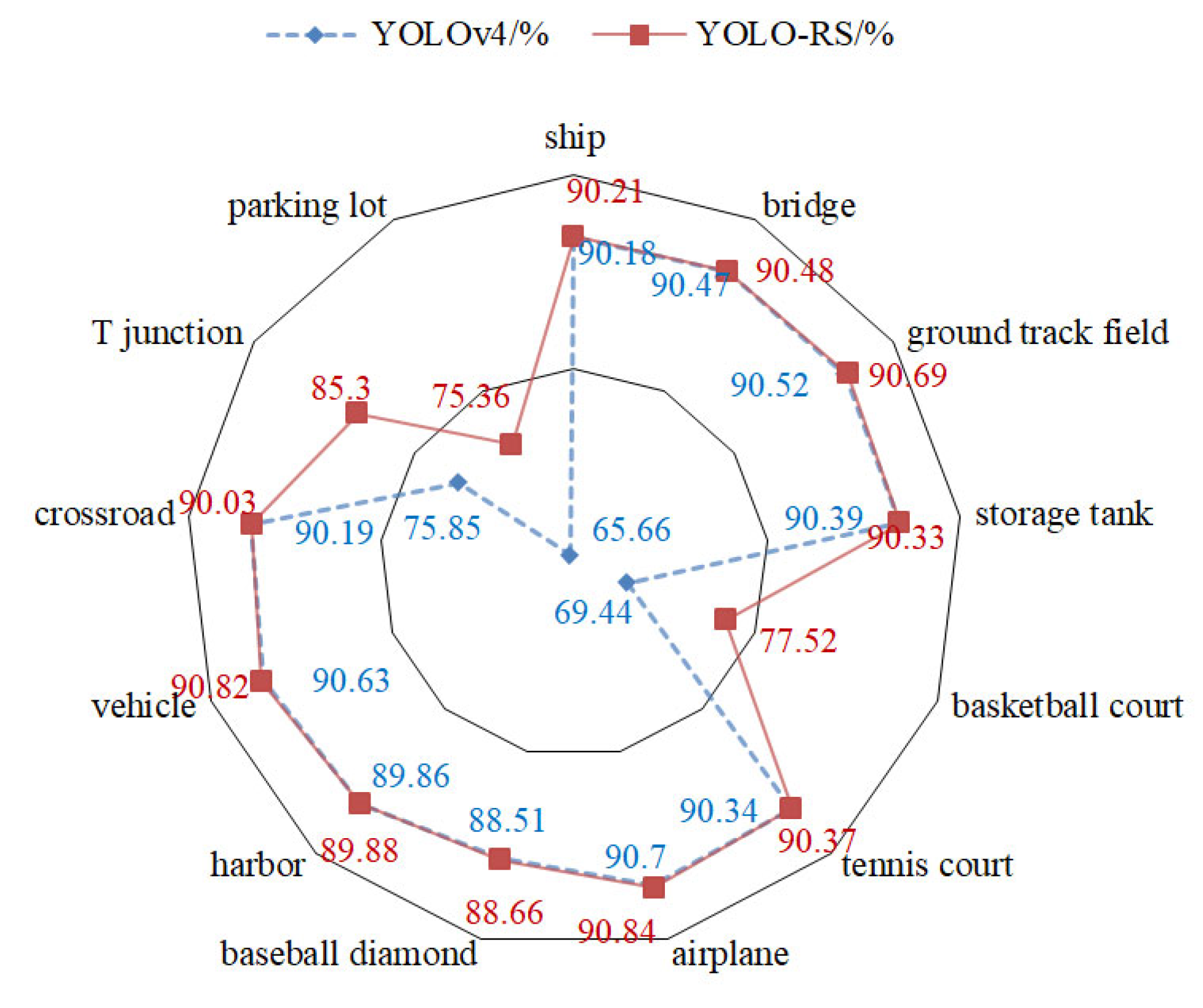
4.6. Single Class Precision Presentation

Figure 9 shows some detection results of YOLO-RS on the TGRS-HRRSD dataset. Figure 10 presents the AP values for each individual class of the original YOLOv4 algorithm and the proposed algorithm on the TGRS-HRRSD dataset. Comparing the detection results of the original YOLOv4 algorithm with the optimized version, most of the class AP values have been effectively improved, except for the storage tank and crossroad categories, which show slight decreases in AP values. Significant improvements in AP values for specific classes are observed in the basketball court, parking lot, and T junction categories, with AP values increasing by 8.08%, 9.70%, and 9.45%, respectively.

The partial detection results of the optimized network on the RSOD dataset are shown in Figure 11. Figure 12 shows the AP values of various categories detected by the original YOLOv4 object detection algorithm and the algorithm proposed in this paper on the RSOD dataset. Compared with the original YOLOv4 object detection algorithm, YOLO-RS has increased mAP by 1.66%. In the detection tasks of two categories, oil tank and playground, the AP values of each single category detected by the original YOLOv4 algorithm and the algorithm proposed in this paper are almost equal on the RSOD dataset. However, in the detection tasks of two categories, airplane and overpass, the optimized algorithm proposed in this paper performs significantly better than the original YOLOv4 object detection algorithm, and its AP values are higher than those of the latter. Therefore, this study proposes that the optimized algorithm has a more competitive performance in detecting airplanes and overpasses.

4.7. Presentation Comparison

Figure 13 shows the comparison of detection results of YOLOv4 and YOLO-RS on the TGRS-HRRSD dataset. The first group of images contains two ground track fields and several basketball courts.

As shown in Figure 13, YOLOv4 missed all basketball court objects while YOLO-RS could detect all basketball court objects well. In the second group of images, YOLOv4 missed some objects while YOLO-RS could recognize all objects in the image. Finally, in the third group of images, YOLOv4 incorrectly detected a crossroad as a T-junction.

Figure 14 shows examples of the detection effect of YOLOv4 and YOLO-RS on remote sensing images in the TGRS-HRRSD dataset.

In the first group of examples in Figure 14, the original YOLOv4 object detection algorithm missed the detection of an airplane with a color attached to its surface. However, the algorithm proposed in this study could identify this airplane object well in the detection task. In the second group of images to be detected, YOLOv4 only detected one playground object while YOLO-RS could detect all objects. Finally, in the third group of examples, YOLOv4 did not recognize the overpass object while YOLO-RS could recognize it.

4.8. Methodology Comparison Experiment

This subsection compares the algorithm proposed in this study, i.e., YOLO-RS, with other mainstream classical algorithms in a comparative experiment under the TGRS-HRRSD dataset and the RSOD dataset. The experiments are compared in terms of both detection accuracy and speed. The main mainstream algorithms include the classical one-stage object detection algorithm and the two-stage object detection algorithm.

Analyzing

Table 4. Algorithm comparison experiments.

Methodology	TGRS-HRRSD		RSOD
	mAP (%)	FPS (f/s)	mAP (%)	FPS (f/s)
Faster R-CNN	81.43	11.67	80.39	11.83
SSD	72.98	26.89	78.28	26.73
YOLOv3	75.06	32.53	82.47	31.97
YOLOv4	85.58	38.16	91.15	38.38
YOLOv5	84.86	49.50	90.91	50.23
YOLO-RS (ours)	87.73	43.45	92.81	43.68

Bold font indicates the optimal values of each metric.

, it is evident that the Faster R-CNN network has the worst detection speed performance among the many models under the two datasets, and, similarly, the detection accuracy performance does not have any advantage over the other one-stage object detection algorithms in the table. Compared to the YOLO series network, the SSD network also poorly performs in terms of detection speed and detection accuracy. Compared to the Faster R-CNN network and the SSD network, the YOLOv3 network has improved detection speed in remote sensing image detection tasks, and the mAP value of the YOLOv3 network is 75.06% under the TGRS-HRRSD dataset, which is lower than the mAP value of 81.43% under the Faster R-CNN network. This is because the YOLOv3 network only uses simple FPN for feature enhancement and fails to fully fuse effective features, resulting in poor detection accuracy. YOLOv4 is the base network used in this paper. It introduces the SPP structure and PANet structure in the process of feature enhancement compared to the YOLOv3 network, while the CSPNet residuals are used to reduce the complexity of the model during feature extraction. YOLOv4 shows improved detection accuracy and speed, with mAP values of 85.58% and 91.15% and detection speeds of 38.16 FPS and 38.38 FPS under the TGRS-HRRSD dataset and RSOD dataset, respectively. YOLOv5 is improved from YOLOv3 by introducing the Focus structure to obtain richer channel information. Although YOLOv5 has a slight advantage in detection speed, it is inferior to the baseline YOLOv4, not to mention YOLO-RS, in terms of detection accuracy in the context of this paper. The mAP of YOLO-RS under the TGRS-HRRSD dataset and the RSOD dataset is higher than that of YOLOv5 by 2.87% and 1.90%, respectively. Therefore, in general, considering the balance of detection speed and accuracy, the baseline selection and method design in this paper are reasonable. The mAP values of YOLO-RS on the TGRS-HRRSD dataset and the RSOD dataset are 87.73% and 92.81%, respectively. Compared with the original YOLOv4 algorithm, they are improved by 2.15% and 1.66%, respectively. The detection speeds are 43.45 FPS and 43.68 FPS, which are improved by 5.29 FPS and 5.30 FPS compared with the original YOLOv4 algorithm. Therefore, YOLO-RS has better detection accuracy and detection speed in remote sensing image object detection tasks and achieves a balance.

5. Discussion

In this paper, we study a series of optimization and improvement works on the original algorithm based on the YOLOv4 object detection algorithm for the characteristics of remote sensing images. Compared with the original object detection algorithm, the new method, YOLO-RS, achieves an improvement in both detection accuracy and detection speed. YOLO-RS was experimentally demonstrated under the TGRS-HRRSD dataset and RSOD dataset, respectively, and both achieved competitive detection results and an effective improvement in detection accuracy and precision, while the comparative experiments combined with mainstream object detection algorithms further verified the applicability and robustness of the YOLO-RS algorithm. However, remote sensing images still exhibited characteristics such as significant variations in object orientation and dense distribution. These factors often lead to overlapping and interfering detection boxes, making it challenging to accurately locate the target object using horizontal detection boxes alone. Consequently, it is worth considering the utilization of rotatable prediction boxes and anchor-free methods in future work to address these issues in object detection algorithms.

References

1. Gagliardi, V.; Tosti, F.; Ciampoli, L.B.; Battagliere, M.L.; D’amato, L.; Alani, A.M.; Benedetto, A. Satellite Remote Sensing and Non-Destructive Testing Methods for Transport Infrastructure Monitoring: Advances, Challenges and Perspectives. Remote Sens. 2023, 15, 418. [Google Scholar] [CrossRef]
2. Gong, J.; Liu, C.; Huang, X. Advances in urban information extraction from high-resolution remote sensing imagery. Sci. China Earth Sci. 2020, 63, 463–475. [Google Scholar] [CrossRef]
3. Orynbaikyzy, A.; Gessner, U.; Conrad, C. Crop type classification using a combination of optical and radar remote sensing data: A review. Int. J. Remote Sens. 2019, 40, 6553–6595. [Google Scholar] [CrossRef]
4. Ghaffarian, S.; Roy, D.; Filatova, T.; Kerle, N. Agent-based modelling of post-disaster recovery with remote sensing data. Int. J. Disaster Risk Reduct. 2021, 60, 102285. [Google Scholar] [CrossRef]
5. Huang, W.; Huang, Y.; Wang, H.; Li, W.; Zhang, L. Local Binary Patterns and Superpixel-Based Multiple Kernels for Hyperspectral Image Classification. IEEE J. Sel. Top. Appl. Earth Obs. Remote Sens. 2020, 13, 4550–4563. [Google Scholar] [CrossRef]
6. Huang, H.; Xu, K.; Shi, G. Joint Multiscale and Multifeature for High-Resolution Remote Sensing Image Scene Classification. Chin. J. Electron. 2020, 48, 1824–1833. [Google Scholar]
7. Zhu, F.; Chen, X.; Chen, S.; Zheng, W.; Ye, W. Relative Margin Induced Support Vector Ordinal Regression. Expert Syst. Appl. 2023, 231, 120766. [Google Scholar] [CrossRef]
8. Zhu, F.; Gao, J.; Yang, J.; Ye, N. Neighborhood Linear Discriminant Analysis. Pattern Recognit. 2022, 123, 108422. [Google Scholar] [CrossRef]
9. Zhu, F.; Zhang, W.; Chen, X.; Gao, X.; Ye, N. Large Margin Distribution Multi-Class Supervised Novelty Detection. Expert Syst. Appl. 2023, 224, 119937. [Google Scholar] [CrossRef]
10. Nie, T.; Han, X.; He, B.; Zhang, L. Ship Detection in Panchromatic Optical Remote Sensing Images Based on Visual Saliency and Multi-Dimensional Feature Description. Remote Sens. 2020, 12, 152. [Google Scholar] [CrossRef] [Green Version]
11. Sha, M.; Li, Y.; Li, A. Improved Faster R-CNN for Aircraft Object Detection in Remote Sensing Images. Nat. Remote Sens. Bull. 2022, 26, 1624–1635. [Google Scholar] [CrossRef]
12. Yang, D.; Mao, Y. Remote Sensing Landslide Target Detection Method Based on Improved Faster R-CNN. J. Appl. Remote Sens. 2022, 16, 044521. [Google Scholar]
13. Wen, G.Q.; Cao, P.; Wang, H.N.; Yang, L.; Zhang, L. MS-SSD: Multi-Scale Single Shot Detector for Ship Detection in Remote Sensing Images. Appl. Intell. 2023, 53, 1586–1604. [Google Scholar] [CrossRef]
14. Qu, Z.F.; Zhu, F.Z.; Qi, C.X. Remote Sensing Image Target Detection: Improvement of the YOLOv3 Model with Auxiliary Networks. Remote Sens. 2021, 13, 3908. [Google Scholar] [CrossRef]
15. Shen, L.; Tao, H.; Ni, Y.; Wang, Y.; Stojanovic, V. Improved YOLOv3 Model with Feature Map Cropping for Multi-Scale Road Object Detection. Meas. Sci. Technol. 2023, 34, 045406. [Google Scholar] [CrossRef]
16. Tutsoy, O.; Tanrikulu, M.Y. Priority and Age-Specific Vaccination Algorithm for Pandemic Diseases: A Comprehensive Parametric Prediction Model. BMC Med. Inform. Decis. Mak. 2022, 22, 4. [Google Scholar] [CrossRef]
17. Bochkovskiy, A.; Wang, C.Y.; Liao, H.Y.M. YOLOv4: Optimal Speed and Accuracy of Object Detection. arXiv 2020, arXiv:2004.10934. [Google Scholar]
18. Zhao, S.; Xu, T.; Wu, X.J.; Hoi, S.C.H. Adaptive Feature Fusion for Visual Object Tracking. Pattern Recognit. 2021, 111, 107679. [Google Scholar] [CrossRef]
19. Wang, C.Y.; Liao, H.Y.M.; Wu, Y.H.; Chen, P.Y.; Hsieh, J.W.; Yeh, I.H. CSPNet: A New Backbone that can Enhance Learning Capability of CNN. In Proceedings of the IEEE International Conference on Computer Vision, Seoul, Republic of Korea, 27 October–2 November 2019. [Google Scholar]
20. Lin, M.; Chen, Q.; Yan, S. Network in Network. arXiv 2013, arXiv:1312.4400. [Google Scholar]
21. Khan, Z.Y.; Niu, Z. CNN with Depthwise Separable Convolutions and Combined Kernels for Rating Prediction. Expert Syst. Appl. 2021, 170, 114528. [Google Scholar] [CrossRef]
22. Sandler, M.; Howard, A.; Zhu, M.; Zhmoginov, A.; Chen, L.C. MobileNetV2: Inverted Residuals and Linear Bottlenecks. In Proceedings of the IEEE Conference on Computer Vision and Pattern Recognition, Salt Lake City, UT, USA, 18–22 June 2018. [Google Scholar]
23. Howard, A.; Sandler, M.; Chu, G.; Chen, L.C.; Chen, B.; Tan, M.; Wang, W.; Zhu, Y.; Pang, R.; Vasudevan, V.; et al. Searching for MobileNetV3. In Proceedings of the IEEE International Conference on Computer Visionand Pattern Recognition, Long Beach, CA, USA, 16–20 June 2019. [Google Scholar]
24. Zhang, X.; Zhou, X.; Lin, M.; Sun, J. ShuffleNet: An Extremely Efficient Convolutional Neural Network for Mobile Devices. In Proceedings of the IEEE Conference on Computer Vision and Pattern Recognition, Honolulu, HI, USA, 21–26 July 2017. [Google Scholar]
25. Han, K.; Wang, Y.; Tian, Q.; Guo, J.; Xu, C.; Xu, C. GhostNet: More Features from Cheap Operations. In Proceedings of the IEEE Conference on Computer Vision and Pattern Recognition, Seattle, WA, USA, 14–19 June 2020. [Google Scholar]
26. Zhang, Y.F.; Ren, W.Q.; Zhang, Z.; Jia, Z.; Wang, L.; Tan, T. Focal and Efficient IOU Loss for Accurate Bounding Box Regression. Neurocomputing 2022, 506, 146–157. [Google Scholar] [CrossRef]
27. Zhang, Y.; Yuan, Y.; Feng, Y.; Lu, X. Hierarchical and Robust Convolutional Neural Network for Very High-Resolution Remote Sensing Object Detection. IEEE Trans. Geosci. Remote Sens. 2019, 57, 5535–5548. [Google Scholar] [CrossRef]
28. Xiao, Z.; Liu, Q.; Tang, G.; Zhai, X. Elliptic Fourier Transformation-Based Histograms of Oriented Gradients for Rotationally Invariant Object Detection in Remote-Sensing Images. Int. J. Remote Sens. 2015, 36, 618–644. [Google Scholar] [CrossRef]
29. Long, Y.; Gong, Y.P.; Xiao, Z.F.; Liu, Q. Accurate Object Localization in Remote Sensing Images Based on Convolutional Neural Networks. IEEE Trans. Geosci. Remote Sens. 2017, 55, 2486–2498. [Google Scholar] [CrossRef]
Figure 1. YOLO-RS network architecture.
Remotesensing 15 03863 g001
Figure 2. Feature enhancement network with ASFF.
Remotesensing 15 03863 g002
Figure 3. SPP with the introduction of a maximum residual connection.
Remotesensing 15 03863 g003
Figure 4. Schematic diagram of OSPP structure.
Remotesensing 15 03863 g004
Figure 5. Schematic diagram of Lightnet.
Remotesensing 15 03863 g005
Figure 6. (a) Normal Convolution; (b) Depthwise Separable Convolution.
Remotesensing 15 03863 g006
Figure 7. Distribution of object categories in TGRS-HRRSD dataset.
Remotesensing 15 03863 g007
Figure 8. Distribution of object categories in the RSOD dataset.
Remotesensing 15 03863 g008
Figure 9. YOLO-RS partial detection results on the TGRS-HRRSD dataset.
Remotesensing 15 03863 g009
Figure 10. The AP of various categories under the TGRS-HRRSD dataset.
Remotesensing 15 03863 g010
Figure 11. YOLO-RS detection results on the RSOD dataset.
Remotesensing 15 03863 g011
Figure 12. The AP of various categories under the RSOD dataset.
Remotesensing 15 03863 g012
Figure 13. Comparison of detection results of YOLOv4 and YOLO-RS on the TGRS-HRRSD dataset.
Remotesensing 15 03863 g013aRemotesensing 15 03863 g013b
Figure 14. Comparison of detection results of YOLOv4 and YOLO-RS on the RSOD dataset.
Remotesensing 15 03863 g014